2.1 Flow decomposition

The boundary-layer velocity, pressure and temperature $\boldsymbol{q}=\{u,v,w,p,\unicode[STIX]{x1D70F}\}$ are decomposed into their mean $\boldsymbol{Q}$ and perturbation $\acute{\boldsymbol{q}}$ as

(2.2) $$\begin{eqnarray}\boldsymbol{q}(\boldsymbol{x},t)=\boldsymbol{Q}(\boldsymbol{x})+\unicode[STIX]{x1D716}\acute{\boldsymbol{q}}(\boldsymbol{x},t).\end{eqnarray}$$

Under the assumption $r\gg 1$ , curvature effects on the mean flow can be neglected (Spall & Malik Reference Spall and Malik1989) and, consequently, at leading order the mean flow behaves as if the plate were flat. Neither a mean streamwise pressure gradient nor a mean spanwise pressure gradient is present. The Dorodnitsyn–Howarth transformation can then be applied to obtain the mean-flow momentum equation ${\mathcal{M}}$ and the energy equation ${\mathcal{E}}$ in similarity form (Stewartson Reference Stewartson1964),

(2.3) $$\begin{eqnarray}\displaystyle & \displaystyle {\mathcal{M}}\!\rceil \;\left(\frac{\unicode[STIX]{x1D707}F^{\prime \prime }}{T}\right)^{\prime }+FF^{\prime \prime }=0, & \displaystyle\end{eqnarray}$$

(2.4) $$\begin{eqnarray}\displaystyle & \displaystyle {\mathcal{E}}\!\rfloor \;\left(\frac{\unicode[STIX]{x1D707}T^{\prime }}{PrT}\right)^{\prime }+M^{2}(\unicode[STIX]{x1D6FE}-1)\frac{\unicode[STIX]{x1D707}{F^{\prime \prime }}^{2}}{T}+FT^{\prime }=0, & \displaystyle\end{eqnarray}$$

where we have introduced the compressible Blasius function $F=F(\unicode[STIX]{x1D702})$ , the temperature $T=T(\unicode[STIX]{x1D702})$ and the dynamic viscosity $\unicode[STIX]{x1D707}(T)=T^{\unicode[STIX]{x1D714}}$ , where $\unicode[STIX]{x1D714}=0.76$ (Stewartson Reference Stewartson1964). The prime $^{\prime }$ indicates the derivative with respect to the independent similarity variable $\unicode[STIX]{x1D702}=\bar{Y}/(2\hat{x})^{1/2}$ , where $\bar{Y}(\hat{x},y)=\int _{0}^{y}1/T(\hat{x},\bar{y})\,\text{d}\bar{y}$ . The Prandtl number, assumed to be constant, is $Pr=0.707$ . The boundary conditions for (2.3) and (2.4) are

(2.5a,b ) $$\begin{eqnarray}\unicode[STIX]{x1D702}=0\!\rceil \;F=F^{\prime }=0,\quad T^{\prime }=0,\end{eqnarray}$$

(2.6a,b ) $$\begin{eqnarray}\unicode[STIX]{x1D702}\rightarrow \infty \!\rfloor \;F^{\prime }\rightarrow 1,\quad T\rightarrow 1.\end{eqnarray}$$

The streamwise velocity $U$ and the wall-normal velocity $V$ of the mean flow are

(2.7a,b ) $$\begin{eqnarray}U=F^{\prime },\quad V=\frac{T(\unicode[STIX]{x1D702}_{c}F^{\prime }-F)}{R(2\hat{x})^{1/2}},\end{eqnarray}$$

where $\unicode[STIX]{x1D702}_{c}(\unicode[STIX]{x1D702})=T^{-1}\int _{0}^{\unicode[STIX]{x1D702}}T(\hat{\unicode[STIX]{x1D702}})\,\text{d}\hat{\unicode[STIX]{x1D702}}$ (Stewartson Reference Stewartson1964). The wall-normal mean velocity $V$ can only be approximated by (2.7) in specific ranges of $\unicode[STIX]{x1D702}$ and $\hat{x}$ , as discussed in appendix A.

2.2 The compressible boundary-region equations with curvature effects

The theoretical framework used herein is a combination of the work of Wu et al. (Reference Wu, Zhao and Luo2011) on incompressible Görtler flows over concave surfaces with the work of Ricco & Wu (Reference Ricco and Wu2007) on compressible Klebanoff modes over flat surfaces. Both papers are extensions of the original theory developed by Leib et al. (Reference Leib, Wundrow and Goldstein1999) for the incompressible flat-plate case.

Before introducing the boundary-region equations it is instructive to discuss the different asymptotic flow regions, represented in figure 1. The flow domain is divided in five main regions: region $\text{FS}$ (free stream) for which $x^{2}+y^{2}\gg 1$ , and regions $\text{I}$ , $\text{II}$ , $\text{III}$ and $\text{IV}$ . Goldstein (Reference Goldstein1978) developed an analytic framework for the description of the free-stream vortical disturbances in region $\text{I}$ . Here, the external disturbances are described as a superposition of inviscid harmonic vortical disturbances which, in the limit $\unicode[STIX]{x1D716}\ll 1$ , can be analysed separately due to the linearity of the problem. As the free-stream vortical disturbances evolve further downstream, the outer flow enters region $\text{IV}$ where the mean flow is still inviscid. Here, the displacement effect caused by the boundary-layer growth and the energy decay due to viscous dissipation are analytically treated (Leib et al. Reference Leib, Wundrow and Goldstein1999). The dynamics of the flow disturbance in these outer regions causes the origin and growth of the perturbation in the viscous regions $\text{II}$ and $\text{III}$ inside the boundary layer. The method of matched-asymptotic expansion is used to link the outer regions $\text{I}$ and $\text{IV}$ with the boundary-layer regions $\text{II}$ and $\text{III}$ . Region $\text{II}$ is governed by the linearized unsteady boundary-layer equations, i.e. the linearized unsteady boundary-region (LUBR) equations with the spanwise diffusion and normal pressure gradient terms neglected. Originally introduced by Kemp (Reference Kemp1951), the LUBR equations are the full Navier–Stokes and continuity equations with the terms pertaining to the streamwise viscous diffusion and the streamwise pressure gradient neglected. This is a rigorous simplification that follows directly from the assumptions $R\rightarrow \infty$ and $k_{x}\rightarrow 0$ . Gulyaev et al. (Reference Gulyaev, Kozlov, Kuzenetsov, Mineev and Sekundov1989), Choudhari (Reference Choudhari1996) and Leib et al. (Reference Leib, Wundrow and Goldstein1999) recognized that the linearized unsteady boundary-layer equations are only appropriate in a small region near the leading edge where the spanwise wavelength $\unicode[STIX]{x1D706}_{z}^{\ast }$ is much larger than the boundary-layer thickness $\unicode[STIX]{x1D6FF}^{\ast }=O((x^{\ast }\unicode[STIX]{x1D708}_{\infty }^{\ast }/U_{\infty }^{\ast })^{1/2})$ . As the boundary layer grows to a thickness comparable with the spanwise wavelength, i.e.  $\unicode[STIX]{x1D6FF}^{\ast }=O(\unicode[STIX]{x1D706}_{z}^{\ast })$ , the spanwise diffusion terms become of the same order as the wall-normal diffusion terms. This occurs in region $\text{III}$ , where the Klebanoff modes in the flat-plate case and the Görtler vortices for flows over concave surfaces are fully developed. The LUBR equations, complemented by rigorous initial and free-stream boundary conditions, must therefore be used to study the flow in region $\text{III}$ . The boundary-layer perturbations are assumed to be periodic in time $t$ and along the spanwise direction $z$ . They are expressed as in Gulyaev et al. (Reference Gulyaev, Kozlov, Kuzenetsov, Mineev and Sekundov1989),

(2.8) $$\begin{eqnarray}\acute{\boldsymbol{q}}(\boldsymbol{x},t)=\text{i}k_{z}\check{w}\left\{R\bar{u},(2\hat{x})^{1/2}\bar{v},\frac{1}{\text{i}k_{z}}\bar{w},\frac{1}{R}\bar{p},R\bar{\unicode[STIX]{x1D70F}}\right\}\text{e}^{\text{i}(k_{z}z-k_{x}R\hat{t})}+\text{c.c.},\end{eqnarray}$$

where $\check{w}\equiv {\hat{w}}^{\infty }+\text{i}k_{z}\hat{v}^{\infty }(k_{x}^{2}+k_{z}^{2})^{-1/2}$ and $\bar{\boldsymbol{q}}(\hat{x},\unicode[STIX]{x1D702})=\{\bar{u},\bar{v},\bar{w},\bar{p},\bar{\unicode[STIX]{x1D70F}}\}(\hat{x},\unicode[STIX]{x1D702})$ .

The full compressible continuity and Navier–Stokes equations in curvilinear coordinates are first simplified using the Lamé coefficients. The mean flow (2.7) and the perturbation flow (2.8) are then introduced into the equations and, taking the limits $R\rightarrow \infty$ and $k_{x}\rightarrow 0$ with $k_{x}\text{R}=O(1)$ , the LUBR equations are obtained:

(2.9) $$\begin{eqnarray}\displaystyle & & \displaystyle {\mathcal{C}}\!\rceil \;\frac{\unicode[STIX]{x1D702}_{c}}{2\hat{x}}\frac{T^{\prime }}{T}\bar{u}+\frac{\unicode[STIX]{x2202}\bar{u}}{\unicode[STIX]{x2202}\hat{x}}-\frac{\unicode[STIX]{x1D702}_{c}}{2\hat{x}}\frac{\unicode[STIX]{x2202}\bar{u}}{\unicode[STIX]{x2202}\unicode[STIX]{x1D702}}-\frac{T^{\prime }}{T^{2}}\bar{v}+\frac{1}{T}\frac{\unicode[STIX]{x2202}\bar{v}}{\unicode[STIX]{x2202}\unicode[STIX]{x1D702}}+\bar{w}+\left(\text{i}k_{x}R\frac{1}{T}-\frac{1}{2\hat{x}}\frac{FT^{\prime }}{T^{2}}\right)\bar{\unicode[STIX]{x1D70F}}-\frac{F^{\prime }}{T}\frac{\unicode[STIX]{x2202}\bar{\unicode[STIX]{x1D70F}}}{\unicode[STIX]{x2202}\hat{x}}\nonumber\\ \displaystyle & & \displaystyle \quad \;\;+\,\frac{1}{2\hat{x}}\frac{F}{T}\frac{\unicode[STIX]{x2202}\bar{\unicode[STIX]{x1D70F}}}{\unicode[STIX]{x2202}\unicode[STIX]{x1D702}}=0,\end{eqnarray}$$

(2.10) $$\begin{eqnarray}\displaystyle & & \displaystyle {\mathcal{X}}|\;\left(-\text{i}k_{x}R-\frac{\unicode[STIX]{x1D702}_{c}}{2\hat{x}}F^{\prime \prime }+k_{z}^{2}\unicode[STIX]{x1D707}T\right)\bar{u}+F^{\prime }\frac{\unicode[STIX]{x2202}\bar{u}}{\unicode[STIX]{x2202}\hat{x}}-\frac{1}{2\hat{x}}\left(F+\frac{\unicode[STIX]{x1D707}^{\prime }T^{\prime }}{T}-\frac{\unicode[STIX]{x1D707}T^{\prime }}{T^{2}}\right)\frac{\unicode[STIX]{x2202}\bar{u}}{\unicode[STIX]{x2202}\unicode[STIX]{x1D702}}-\frac{1}{2\hat{x}}\frac{\unicode[STIX]{x1D707}}{T}\frac{\unicode[STIX]{x2202}^{2}\bar{u}}{\unicode[STIX]{x2202}\unicode[STIX]{x1D702}^{2}}\nonumber\\ \displaystyle & & \displaystyle \quad \;\;+\,\frac{F^{\prime \prime }}{T}\bar{v}+\frac{1}{2\hat{x}T}\left(FF^{\prime \prime }-\unicode[STIX]{x1D707}^{\prime \prime }F^{\prime \prime }T^{\prime }+\frac{\unicode[STIX]{x1D707}^{\prime }F^{\prime \prime }T^{\prime }}{T}-\unicode[STIX]{x1D707}^{\prime }F^{\prime \prime \prime }\right)\bar{\unicode[STIX]{x1D70F}}-\frac{1}{2\hat{x}}\frac{\unicode[STIX]{x1D707}^{\prime }F^{\prime \prime }}{T}\frac{\unicode[STIX]{x2202}\bar{\unicode[STIX]{x1D70F}}}{\unicode[STIX]{x2202}\unicode[STIX]{x1D702}}=0,\end{eqnarray}$$

(2.11) $$\begin{eqnarray}\displaystyle & & \displaystyle {\mathcal{Y}}|\;\frac{1}{4\hat{x}^{2}}[\unicode[STIX]{x1D702}_{c}(FT^{\prime }-F^{\prime }T)-\unicode[STIX]{x1D702}_{c}^{2}F^{\prime \prime }T+FT]\bar{u}+\frac{\unicode[STIX]{x1D707}^{\prime }T^{\prime }}{3\hat{x}}\frac{\unicode[STIX]{x2202}\bar{u}}{\unicode[STIX]{x2202}\hat{x}}-\frac{\unicode[STIX]{x1D707}}{6\hat{x}}\frac{\unicode[STIX]{x2202}^{2}\bar{u}}{\unicode[STIX]{x2202}\hat{x}\unicode[STIX]{x2202}\unicode[STIX]{x1D702}}+\frac{\unicode[STIX]{x1D702}_{c}\unicode[STIX]{x1D707}}{12\hat{x}^{2}}\frac{\unicode[STIX]{x2202}^{2}\bar{u}}{\unicode[STIX]{x2202}\unicode[STIX]{x1D702}^{2}}\nonumber\\ \displaystyle & & \displaystyle \quad \;+\,\frac{1}{12\hat{x}^{2}}\left(\unicode[STIX]{x1D702}_{c}\unicode[STIX]{x1D707}^{\prime }T^{\prime }+\unicode[STIX]{x1D707}-\frac{\unicode[STIX]{x1D702}_{c}\unicode[STIX]{x1D707}T^{\prime }}{T}\right)\frac{\unicode[STIX]{x2202}\bar{u}}{\unicode[STIX]{x2202}\unicode[STIX]{x1D702}}+\left[\frac{1}{2\hat{x}}\left(F^{\prime }+\unicode[STIX]{x1D702}_{c}F^{\prime \prime }-\frac{FT^{\prime }}{T}\right)-\text{i}k_{x}R+k_{z}^{2}\unicode[STIX]{x1D707}T\right]\bar{v}\nonumber\\ \displaystyle & & \displaystyle \quad \;+\,F^{\prime }\frac{\unicode[STIX]{x2202}\bar{v}}{\unicode[STIX]{x2202}\hat{x}}+\frac{1}{\hat{x}}\left[\frac{2}{3T}\left(\frac{\unicode[STIX]{x1D707}T^{\prime }}{T}-\unicode[STIX]{x1D707}^{\prime }T^{\prime }\right)-\frac{F}{2}\right]\frac{\unicode[STIX]{x2202}\bar{v}}{\unicode[STIX]{x2202}\unicode[STIX]{x1D702}}-\frac{2}{3\hat{x}}\frac{\unicode[STIX]{x1D707}}{T}\frac{\unicode[STIX]{x2202}^{2}\bar{v}}{\unicode[STIX]{x2202}\unicode[STIX]{x1D702}^{2}}+\frac{\unicode[STIX]{x1D707}^{\prime }T^{\prime }}{3\hat{x}}\bar{w}-\frac{\unicode[STIX]{x1D707}}{6\hat{x}}\frac{\unicode[STIX]{x2202}\bar{w}}{\unicode[STIX]{x2202}\unicode[STIX]{x1D702}}+\frac{1}{2\hat{x}}\frac{\unicode[STIX]{x2202}\bar{p}}{\unicode[STIX]{x2202}\unicode[STIX]{x1D702}}\nonumber\\ \displaystyle & & \displaystyle \quad \;+\,\left[\frac{1}{3\hat{x}^{2}T}\left(\unicode[STIX]{x1D707}^{\prime \prime }F{T^{\prime }}^{2}-\frac{\unicode[STIX]{x1D707}^{\prime }F{T^{\prime }}^{2}}{T}+\unicode[STIX]{x1D707}^{\prime }FT^{\prime \prime }+\unicode[STIX]{x1D707}^{\prime }F^{\prime }T^{\prime }\right)-\frac{1}{4\hat{x}^{2}}\left(F^{\prime }F-\unicode[STIX]{x1D702}_{c}{F^{\prime }}^{2}-\unicode[STIX]{x1D702}_{c}FF^{\prime \prime }\right.\right.\nonumber\\ \displaystyle & & \displaystyle \quad \;+\left.\left.\frac{F^{2}T^{\prime }}{T}+\unicode[STIX]{x1D707}^{\prime }F^{\prime \prime }+\unicode[STIX]{x1D702}_{c}\unicode[STIX]{x1D707}^{\prime \prime }F^{\prime \prime }T^{\prime }-\frac{\unicode[STIX]{x1D702}_{c}\unicode[STIX]{x1D707}^{\prime }F^{\prime \prime }T^{\prime }}{T}+\unicode[STIX]{x1D702}_{c}F^{\prime \prime \prime }\unicode[STIX]{x1D707}^{\prime }\right)\right]\bar{\unicode[STIX]{x1D70F}}+\frac{\unicode[STIX]{x1D707}^{\prime }}{\hat{x}^{2}}\left(\frac{FT^{\prime }}{3T}-\frac{\unicode[STIX]{x1D702}_{c}F^{\prime \prime }}{4}\right)\frac{\unicode[STIX]{x2202}\bar{\unicode[STIX]{x1D70F}}}{\unicode[STIX]{x2202}\unicode[STIX]{x1D702}}\nonumber\\ \displaystyle & & \displaystyle \quad \;-\,\frac{\unicode[STIX]{x1D707}^{\prime }F^{\prime \prime }}{2\hat{x}}\frac{\unicode[STIX]{x2202}\bar{\unicode[STIX]{x1D70F}}}{\unicode[STIX]{x2202}\hat{x}}+\displaystyle \frac{G}{(2\hat{x})^{1/2}}\left(2F^{\prime }\bar{u}-\frac{{F^{\prime }}^{2}}{T}\bar{\unicode[STIX]{x1D70F}}\right)=0,\end{eqnarray}$$

(2.12) $$\begin{eqnarray}\displaystyle & & \displaystyle {\mathcal{Z}}|\;-\frac{k_{z}^{2}\unicode[STIX]{x1D702}_{c}\unicode[STIX]{x1D707}^{\prime }TT^{\prime }}{2\hat{x}}\bar{u}+\frac{k_{z}^{2}\unicode[STIX]{x1D707}T}{3}\frac{\unicode[STIX]{x2202}\bar{u}}{\unicode[STIX]{x2202}\hat{x}}-\frac{k_{z}^{2}\unicode[STIX]{x1D702}_{c}\unicode[STIX]{x1D707}T}{6\hat{x}}\frac{\unicode[STIX]{x2202}\bar{u}}{\unicode[STIX]{x2202}\unicode[STIX]{x1D702}}+k_{z}^{2}\unicode[STIX]{x1D707}^{\prime }T^{\prime }\bar{v}+\frac{k_{z}^{2}\unicode[STIX]{x1D707}}{3}\frac{\unicode[STIX]{x2202}\bar{v}}{\unicode[STIX]{x2202}\unicode[STIX]{x1D702}}\nonumber\\ \displaystyle & & \displaystyle \quad \;\;+\,\left(\frac{4}{3}k_{z}^{2}\unicode[STIX]{x1D707}T-\text{i}k_{x}R\right)\bar{w}+F^{\prime }\frac{\unicode[STIX]{x2202}\bar{w}}{\unicode[STIX]{x2202}\hat{x}}+\frac{1}{2\hat{x}}\left(\frac{\unicode[STIX]{x1D707}T^{\prime }}{T^{2}}-F-\frac{\unicode[STIX]{x1D707}^{\prime }T^{\prime }}{T}\right)\frac{\unicode[STIX]{x2202}\bar{w}}{\unicode[STIX]{x2202}\unicode[STIX]{x1D702}}-\frac{1}{2\hat{x}}\frac{\unicode[STIX]{x1D707}}{T}\frac{\unicode[STIX]{x2202}^{2}\bar{w}}{\unicode[STIX]{x2202}\unicode[STIX]{x1D702}^{2}}\nonumber\\ \displaystyle & & \displaystyle \quad \;\;-\,k_{z}^{2}T\bar{p}+\frac{k_{z}^{2}}{3\hat{x}}\unicode[STIX]{x1D707}^{\prime }FT^{\prime }\bar{\unicode[STIX]{x1D70F}}=0,\end{eqnarray}$$

(2.13) $$\begin{eqnarray}\displaystyle & & \displaystyle {\mathcal{E}}\!\rfloor \;-\frac{\unicode[STIX]{x1D702}_{c}}{2\hat{x}}T^{\prime }\bar{u}+\frac{T^{\prime }}{T}\bar{v}+\left[\frac{FT^{\prime }}{2\hat{x}T}-\text{i}k_{x}R+\frac{k_{z}^{2}\unicode[STIX]{x1D707}T}{Pr}-\frac{1}{2\hat{x}Pr}\frac{\unicode[STIX]{x2202}}{\unicode[STIX]{x2202}\unicode[STIX]{x1D702}}\left(\frac{\unicode[STIX]{x1D707}^{\prime }T^{\prime }}{T}\right)\right]\bar{\unicode[STIX]{x1D70F}}+F^{\prime }\frac{\unicode[STIX]{x2202}\bar{\unicode[STIX]{x1D70F}}}{\unicode[STIX]{x2202}\hat{x}}\nonumber\\ \displaystyle & & \displaystyle \quad \;\;+\,\frac{1}{2\hat{x}}\left(\frac{\unicode[STIX]{x1D707}T^{\prime }}{PrT^{2}}-F-\frac{2\unicode[STIX]{x1D707}^{\prime }T^{\prime }}{PrT}\right)\frac{\unicode[STIX]{x2202}\bar{\unicode[STIX]{x1D70F}}}{\unicode[STIX]{x2202}\unicode[STIX]{x1D702}}-\frac{1}{2\hat{x}Pr}\frac{\unicode[STIX]{x1D707}}{T}\frac{\unicode[STIX]{x2202}^{2}\bar{\unicode[STIX]{x1D70F}}}{\unicode[STIX]{x2202}\unicode[STIX]{x1D702}^{2}}\nonumber\\ \displaystyle & & \displaystyle \quad \;\;-\,M^{2}\frac{\unicode[STIX]{x1D6FE}-1}{\hat{x}T}\left(\unicode[STIX]{x1D707}F^{\prime \prime }\frac{\unicode[STIX]{x2202}\bar{u}}{\unicode[STIX]{x2202}\unicode[STIX]{x1D702}}+\frac{\unicode[STIX]{x1D707}^{\prime }{F^{\prime \prime }}^{2}}{2}\bar{\unicode[STIX]{x1D70F}}\right)=0,\end{eqnarray}$$

where ${\mathcal{C}}$ , ${\mathcal{X}}$ , ${\mathcal{Y}}$ , ${\mathcal{Z}}$ , ${\mathcal{E}}$ indicate the continuity, $x$ -momentum, $y$ -momentum, $z$ -momentum and energy equations. The prime $^{\prime }$ represents differentiation with respect to the independent variable. The equations of Ricco & Wu (Reference Ricco and Wu2007) for the compressible flow over a flat surface and of Wu et al. (Reference Wu, Zhao and Luo2011) for the incompressible flow over a concave surface are recovered by setting $G=0$ and $M=0$ , respectively. Curvature effects derive from the centrifugal force and only appear in the convective terms of the ${\mathcal{Y}}$ equation (2.11). These terms, boxed in (2.11), are proportional to the Görtler number $G$ and, in the compressible case, also include the temperature perturbation (El-Hady & Verma Reference El-Hady and Verma1983; Hall & Malik Reference Hall and Malik1989). The LUBR equations are parabolic along the streamwise direction and are influenced by $G$ , $k_{y}$ , $k_{x}R$ and $M$ , which account for the effects of curvature, ratio of the free-stream spanwise wavelength to the wall-normal wavelength, frequency and compressibility, respectively.

The streamwise velocity $\bar{u}$ and the temperature perturbation $\bar{\unicode[STIX]{x1D70F}}$ inside the boundary layer tend to zero as the free stream is approached because they amplify inside the boundary layer to an order of magnitude larger than the corresponding free-stream disturbances (Ricco & Wu Reference Ricco and Wu2007). Therefore, the boxed curvature terms in (2.11) can be neglected as $\unicode[STIX]{x1D702}\rightarrow \infty$ and we recover the free-stream boundary conditions used by Ricco & Wu (Reference Ricco and Wu2007):

(2.14) $$\begin{eqnarray}\displaystyle & \displaystyle \unicode[STIX]{x1D702}=0\!\rceil \;\bar{u}=\bar{v}=\bar{w}=\frac{\unicode[STIX]{x2202}\bar{\unicode[STIX]{x1D70F}}}{\unicode[STIX]{x2202}\unicode[STIX]{x1D702}}=0, & \displaystyle\end{eqnarray}$$

(2.15) $$\begin{eqnarray}\displaystyle & \displaystyle \unicode[STIX]{x1D702}\rightarrow \infty \!\rfloor \;\bar{u}\rightarrow 0, & \displaystyle\end{eqnarray}$$

(2.16) $$\begin{eqnarray}\displaystyle & \displaystyle \frac{\unicode[STIX]{x2202}\bar{v}}{\unicode[STIX]{x2202}\unicode[STIX]{x1D702}}+|k_{z}|(2\hat{x})^{1/2}\bar{v}\rightarrow -\text{e}^{\text{i}[k_{x}R\hat{x}+k_{y}(2\hat{x})^{1/2}(\unicode[STIX]{x1D702}-\unicode[STIX]{x1D6FD}_{c})]-(k_{y}^{2}+k_{z}^{2})\hat{x}}, & \displaystyle\end{eqnarray}$$

(2.17) $$\begin{eqnarray}\displaystyle & \displaystyle \frac{\unicode[STIX]{x2202}\bar{w}}{\unicode[STIX]{x2202}\unicode[STIX]{x1D702}}+|k_{z}|(2\hat{x})^{1/2}\bar{w}\rightarrow \text{i}k_{y}(2\hat{x})^{1/2}\text{e}^{\text{i}[k_{x}R\hat{x}+k_{y}(2\hat{x})^{1/2}(\unicode[STIX]{x1D702}-\unicode[STIX]{x1D6FD}_{c})]-(k_{y}^{2}+k_{z}^{2})\hat{x}}, & \displaystyle\end{eqnarray}$$

(2.18) $$\begin{eqnarray}\displaystyle & \displaystyle \frac{\unicode[STIX]{x2202}\bar{p}}{\unicode[STIX]{x2202}\unicode[STIX]{x1D702}}+|k_{z}|(2\hat{x})^{1/2}\bar{p}\rightarrow 0, & \displaystyle\end{eqnarray}$$

(2.19) $$\begin{eqnarray}\displaystyle & \displaystyle \bar{\unicode[STIX]{x1D70F}}\rightarrow 0, & \displaystyle\end{eqnarray}$$

where compressibility effects are taken into account by the parameter $\unicode[STIX]{x1D6FD}_{c}(M)\equiv \lim _{\unicode[STIX]{x1D702}\rightarrow \infty }(\unicode[STIX]{x1D702}-F)$ , which is computed numerically (Ricco, Tran & Ye Reference Ricco, Tran and Ye2009). Since curvature effects are also negligible in the limit $\hat{x}\rightarrow 0$ , the initial conditions of Ricco & Wu (Reference Ricco and Wu2007) apply:

(2.20) $$\begin{eqnarray}\hat{x}\rightarrow 0\!]\;\bar{u}\rightarrow 2\hat{x}U_{0}+(2\hat{x})^{3/2}U_{1},\end{eqnarray}$$

(2.21) $$\begin{eqnarray}\displaystyle \bar{v} & \rightarrow & \displaystyle V_{0}+(2\hat{x})^{1/2}V_{1}-\left[V_{c}-\frac{1}{2}g_{1}|k_{z}|(2\hat{x})^{1/2}\right]\text{e}^{-|k_{z}|(2\hat{x})^{1/2}\bar{\unicode[STIX]{x1D702}}}\nonumber\\ \displaystyle & & \displaystyle +\,\frac{\text{i}}{(k_{y}-\text{i}|k_{z}|)(2\hat{x})^{1/2}}[\text{e}^{\text{i}k_{y}(2\hat{x})^{1/2}\bar{\unicode[STIX]{x1D702}}-(k_{y}^{2}+k_{z}^{2})\hat{x}}-\text{e}^{-|k_{z}|(2\hat{x})^{1/2}\bar{\unicode[STIX]{x1D702}}}]-\bar{v}_{c},\end{eqnarray}$$

(2.22) $$\begin{eqnarray}\displaystyle \bar{w} & \rightarrow & \displaystyle W_{0}+(2\hat{x})^{1/2}W_{1}-V_{c}|k_{z}|(2\hat{x})^{1/2}\text{e}^{-|k_{z}|(2\hat{x})^{1/2}\bar{\unicode[STIX]{x1D702}}}\nonumber\\ \displaystyle & & \displaystyle +\,\frac{1}{k_{y}-\text{i}|k_{z}|}[k_{y}\text{e}^{\text{i}k_{y}(2\hat{x})^{1/2}\bar{\unicode[STIX]{x1D702}}-(k_{y}^{2}+k_{z}^{2})\hat{x}}-\text{i}|k_{z}|\text{e}^{-|k_{z}|(2\hat{x})^{1/2}\bar{\unicode[STIX]{x1D702}}}]-\bar{w}_{c},\end{eqnarray}$$

(2.23) $$\begin{eqnarray}\displaystyle & \displaystyle \bar{p}\rightarrow \frac{P_{0}}{(2\hat{x})^{1/2}}+P_{1}+\left[g_{1}-\frac{V_{c}}{|k_{z}|(2\hat{x})^{1/2}}\right]\text{e}^{-|k_{z}|(2\hat{x})^{1/2}\bar{\unicode[STIX]{x1D702}}}-\bar{p}_{c}, & \displaystyle\end{eqnarray}$$

(2.24) $$\begin{eqnarray}\displaystyle & \displaystyle \bar{\unicode[STIX]{x1D70F}}\rightarrow 2\hat{x}T_{0}+(2\hat{x})^{3/2}T_{1}, & \displaystyle\end{eqnarray}$$

where $\bar{\unicode[STIX]{x1D702}}\equiv \unicode[STIX]{x1D702}-\unicode[STIX]{x1D6FD}_{c}$ . Appendix A further discusses the ranges of validity of the outer boundary conditions (2.15)–(2.19) and of the initial conditions (2.20)–(2.24) in terms of $\unicode[STIX]{x1D702}$ and $\hat{x}$ . The common parts $\bar{v}_{c}$ , $\bar{w}_{c}$ and $\bar{p}_{c}$ , the constants $g_{1}$ and $V_{c}$ and the solutions $U_{0},V_{0},W_{0},P_{0},T_{0},U_{1},V_{1},W_{1},P_{1},T_{1}$ are derived in appendix B. The numerical procedure for solving the LUBR equations is described in appendix C. To stress the importance of receptivity, we note that the solution is influenced by $k_{y}$ only through the initial and boundary conditions as $k_{y}$ does not appear in the LUBR equations (2.9)–(2.13).

2.3 The eigenvalue equations with curvature effects

Because of the inviscid unbalance between the centrifugal force and the wall-normal pressure, the Görtler instability exhibits an exponential streamwise amplification. Following the work of Wu et al. (Reference Wu, Zhao and Luo2011), we can take advantage of this property by adopting a simplified mathematical framework based on an additional decomposition of the quantities defined in (2.8),

(2.25) $$\begin{eqnarray}\bar{\boldsymbol{q}}(\hat{x},\unicode[STIX]{x1D702})=\{\bar{u},\bar{v},\bar{w},\bar{p},\bar{\unicode[STIX]{x1D70F}}\}\equiv \widetilde{\boldsymbol{q}}(\unicode[STIX]{x1D702})\text{e}^{\int ^{\hat{x}}\unicode[STIX]{x1D70E}_{EV}(x)\,\text{d}x},\end{eqnarray}$$

where $\widetilde{\boldsymbol{q}}=\{\widetilde{u},\widetilde{v},\widetilde{w},\widetilde{p},\widetilde{\unicode[STIX]{x1D70F}}\}$ and $\unicode[STIX]{x1D70E}_{EV}=\unicode[STIX]{x1D70E}_{EV,Re}+\text{i}\unicode[STIX]{x1D70E}_{EV,Im}$ is a complex function whose real part $\unicode[STIX]{x1D70E}_{EV,Re}(\hat{x})$ is the local growth rate and the imaginary part $\unicode[STIX]{x1D70E}_{EV,Im}(\hat{x})$ is proportional to the streamwise wavenumber of the boundary-layer perturbation, i.e.

(2.26) $$\begin{eqnarray}k_{x,EV}(\hat{x})=\frac{1}{\hat{x}}\int ^{\hat{x}}\unicode[STIX]{x1D70E}_{EV}(x)\,\text{d}x.\end{eqnarray}$$

Expression (2.25) is a local eigenvalue (EV) decomposition, i.e. valid at a specified streamwise location, which implies that the streamwise dependence of the perturbation is absorbed in $\unicode[STIX]{x1D70E}(\hat{x})$ , while the wall-normal variation is distilled in $\widetilde{\boldsymbol{q}}(\unicode[STIX]{x1D702})$ . The EV perturbation (2.25) is only defined within an undetermined amplitude that can only be found through the receptivity analysis, i.e. by accounting for the influence of the free-stream disturbance. Nevertheless, upon comparison with the LUBR solution, the EV approach identifies the streamwise locations where the perturbation exhibits exponential growth and where its growth rate and streamwise length scale are not influenced by the initial and free-stream boundary conditions.

By substituting (2.25) into (2.9)–(2.13) we obtain the non-parallel EV system of equations, which preserves the growing nature of the boundary-layer mean flow. The equations can be further simplified by invoking the $\unicode[STIX]{x1D702}$ -based parallel mean-flow assumption, which implies $V=0$ , and by taking the limit $\hat{x}\gg 1$ (Wu et al. Reference Wu, Zhao and Luo2011). For numerical reasons, the system of ordinary differential equations is written as a system of first-order equations by introducing three new variables,

(2.27a-c ) $$\begin{eqnarray}\widetilde{f}(\unicode[STIX]{x1D702})\equiv {\displaystyle \frac{\unicode[STIX]{x2202}\widetilde{u}}{\unicode[STIX]{x2202}\unicode[STIX]{x1D702}}},\quad \widetilde{g}(\unicode[STIX]{x1D702})\equiv {\displaystyle \frac{\unicode[STIX]{x2202}\widetilde{w}}{\unicode[STIX]{x2202}\unicode[STIX]{x1D702}}},\quad \widetilde{h}(\unicode[STIX]{x1D702})\equiv {\displaystyle \frac{\unicode[STIX]{x2202}\widetilde{\unicode[STIX]{x1D70F}}}{\unicode[STIX]{x2202}\unicode[STIX]{x1D702}}}.\end{eqnarray}$$

The non-parallel compressible EV equations are given in the following, where the terms between $\langle \hspace{2.22198pt}\rangle$ can be neglected under the parallel-flow assumption because they arise from the wall-normal velocity $V$ given in (2.7).

(2.28) $$\begin{eqnarray}{\mathcal{C}}\!\rceil \;\frac{\unicode[STIX]{x2202}\widetilde{v}}{\unicode[STIX]{x2202}\unicode[STIX]{x1D702}}=(\unicode[STIX]{x1D70E}F^{\prime }-\text{i}k_{x}R)\widetilde{\unicode[STIX]{x1D70F}}-\unicode[STIX]{x1D70E}T\widetilde{u}+\widetilde{v}\frac{T^{\prime }}{T}-T\widetilde{w}+\left\langle \frac{FT^{\prime }}{2\hat{x}T}\widetilde{\unicode[STIX]{x1D70F}}-\frac{\unicode[STIX]{x1D702}_{c}}{2\hat{x}}T^{\prime }\widetilde{u}-\frac{F}{2\hat{x}}\widetilde{h}+\frac{\unicode[STIX]{x1D702}_{c}T}{2\hat{x}}\widetilde{f}\right\rangle ,\end{eqnarray}$$

(2.29) $$\begin{eqnarray}\displaystyle {\mathcal{X}}|\;\frac{\unicode[STIX]{x2202}\widetilde{f}}{\unicode[STIX]{x2202}\unicode[STIX]{x1D702}} & = & \displaystyle \left(-\text{i}k_{x}R\frac{2\hat{x}T}{\unicode[STIX]{x1D707}}+2\hat{x}\unicode[STIX]{x1D70E}\frac{F^{\prime }T}{\unicode[STIX]{x1D707}}+2\hat{x}k_{z}^{2}T^{2}\right)\widetilde{u}-\frac{F^{\prime \prime }\unicode[STIX]{x1D707}^{\prime }}{\unicode[STIX]{x1D707}}\widetilde{h}+\frac{2\hat{x}F^{\prime \prime }}{\unicode[STIX]{x1D707}}\widetilde{v}-\left(\frac{\unicode[STIX]{x1D707}^{\prime }T^{\prime }}{\unicode[STIX]{x1D707}}-\frac{T^{\prime }}{T}\right)\widetilde{f}\nonumber\\ \displaystyle & & \displaystyle +\,\left(\frac{\unicode[STIX]{x1D707}^{\prime }F^{\prime \prime }T^{\prime }}{\unicode[STIX]{x1D707}T}-\frac{\unicode[STIX]{x1D707}^{\prime \prime }F^{\prime \prime }T^{\prime }}{\unicode[STIX]{x1D707}}-\frac{\unicode[STIX]{x1D707}^{\prime }F^{\prime \prime \prime }}{\unicode[STIX]{x1D707}}\right)\widetilde{\unicode[STIX]{x1D70F}}+\left\langle \frac{FF^{\prime \prime }}{\unicode[STIX]{x1D707}}\widetilde{\unicode[STIX]{x1D70F}}-\frac{\unicode[STIX]{x1D702}_{c}F^{\prime \prime }T}{\unicode[STIX]{x1D707}}\widetilde{u}-\frac{FT}{\unicode[STIX]{x1D707}}\widetilde{f}\right\rangle ,\end{eqnarray}$$

(2.30) $$\begin{eqnarray}\displaystyle {\mathcal{Y}}|\;\frac{\unicode[STIX]{x2202}\widetilde{p}}{\unicode[STIX]{x2202}\unicode[STIX]{x1D702}} & = & \displaystyle -\unicode[STIX]{x1D70E}\unicode[STIX]{x1D707}\widetilde{f}-2\unicode[STIX]{x1D70E}T^{\prime }\left(\unicode[STIX]{x1D707}^{\prime }+\frac{2}{3}\frac{\unicode[STIX]{x1D707}}{T}\right)\widetilde{u}+2\hat{x}\left(\text{i}k_{x}R-k_{z}^{2}\unicode[STIX]{x1D707}T-\unicode[STIX]{x1D70E}F^{\prime }\right)\widetilde{v}-\unicode[STIX]{x1D707}\widetilde{g}\nonumber\\ \displaystyle & & \displaystyle +\,\left(F^{\prime \prime }\unicode[STIX]{x1D707}^{\prime }\unicode[STIX]{x1D70E}+\frac{4}{3}\frac{\unicode[STIX]{x1D707}^{\prime }T^{\prime }F^{\prime }\unicode[STIX]{x1D70E}}{T}-\frac{4}{3}\frac{\unicode[STIX]{x1D707}F^{\prime \prime }\unicode[STIX]{x1D70E}}{T}-\frac{4}{3}\text{i}k_{x}R\frac{\unicode[STIX]{x1D707}^{\prime }T^{\prime }}{T}\right)\widetilde{\unicode[STIX]{x1D70F}}+\frac{4}{3}\frac{\unicode[STIX]{x1D707}}{T}\left(\unicode[STIX]{x1D70E}F^{\prime }-\text{i}k_{x}R\right)\widetilde{h}\nonumber\\ \displaystyle & & \displaystyle -\,2T^{\prime }\left(\unicode[STIX]{x1D707}^{\prime }+\frac{2}{3}\frac{\unicode[STIX]{x1D707}}{T}\right)\widetilde{w}+(2\hat{x})^{1/2}GF^{\prime }\left(\frac{F^{\prime }}{T}\widetilde{\unicode[STIX]{x1D70F}}-2\widetilde{u}\right)+\left\langle \frac{\unicode[STIX]{x1D707}}{2\hat{x}}\widetilde{f}+\left(-\text{i}k_{x}R\unicode[STIX]{x1D702}_{c}T\vphantom{\frac{\unicode[STIX]{x1D702}_{c}FT^{\prime }}{\hat{x}}}\right.\vphantom{\frac{\unicode[STIX]{x2202}\widetilde{h}}{\unicode[STIX]{x2202}\unicode[STIX]{x1D702}}}\right.\nonumber\\ \displaystyle & & \displaystyle +\,\unicode[STIX]{x1D70E}\unicode[STIX]{x1D702}_{c}F^{\prime }T+k_{z}^{2}\unicode[STIX]{x1D702}_{c}\unicode[STIX]{x1D707}T^{2}-\frac{2\unicode[STIX]{x1D702}_{c}}{3\hat{x}}\frac{\unicode[STIX]{x1D707}^{\prime }{T^{\prime }}^{2}}{T}+\frac{2\unicode[STIX]{x1D702}_{c}}{3\hat{x}}\frac{\unicode[STIX]{x1D707}{T^{\prime }}^{2}}{T^{2}}-\frac{2}{3\hat{x}}\frac{\unicode[STIX]{x1D707}T^{\prime }}{T}-\frac{2\unicode[STIX]{x1D702}_{c}}{3\hat{x}}\frac{\unicode[STIX]{x1D707}T^{\prime \prime }}{T}+\frac{\unicode[STIX]{x1D702}_{c}}{2\hat{x}}F^{\prime }T\nonumber\\ \displaystyle & & \displaystyle -\left.\frac{FT}{2\hat{x}}-\frac{\unicode[STIX]{x1D702}_{c}FT^{\prime }}{\hat{x}}-\unicode[STIX]{x1D70E}FT\right)\widetilde{u}+\left(\frac{4}{3}\frac{\unicode[STIX]{x1D707}^{\prime }{T^{\prime }}^{2}}{T^{2}}-\frac{4}{3}\frac{\unicode[STIX]{x1D707}{T^{\prime }}^{2}}{T^{3}}+\frac{4}{3}\frac{\unicode[STIX]{x1D707}T^{\prime \prime }}{T^{2}}-F^{\prime }+2\frac{FT^{\prime }}{T}\right)\widetilde{v}\nonumber\\ \displaystyle & & \displaystyle +\,\left(\frac{\unicode[STIX]{x1D707}^{\prime }F^{\prime \prime }}{2\hat{x}}-\frac{2}{3\hat{x}}\frac{\unicode[STIX]{x1D707}^{\prime \prime }F{T^{\prime }}^{2}}{T}+\frac{4}{3\hat{x}}\frac{\unicode[STIX]{x1D707}^{\prime }F{T^{\prime }}^{2}}{T^{2}}-\frac{2}{3\hat{x}}\frac{\unicode[STIX]{x1D707}^{\prime }FT^{\prime \prime }}{T}-\frac{2}{3\hat{x}}\frac{\unicode[STIX]{x1D707}^{\prime }F^{\prime }T^{\prime }}{T}-\frac{2}{3\hat{x}}\frac{\unicode[STIX]{x1D707}F{T^{\prime }}^{2}}{T^{3}}\right.\nonumber\\ \displaystyle & & \displaystyle +\left.\frac{2}{3\hat{x}}\frac{\unicode[STIX]{x1D707}F^{\prime }T^{\prime }}{T^{2}}+\frac{2}{3\hat{x}}\frac{\unicode[STIX]{x1D707}FT^{\prime \prime }}{T^{2}}-\text{i}k_{x}RF+\unicode[STIX]{x1D70E}FF^{\prime }+\frac{FF^{\prime }}{2\hat{x}}+\frac{1}{2\hat{x}}\frac{2F^{2}T^{\prime }}{T}-\frac{\unicode[STIX]{x1D702}_{c}{F^{\prime }}^{2}}{2\hat{x}}\right)\widetilde{\unicode[STIX]{x1D70F}}\nonumber\\ \displaystyle & & \displaystyle +\left.\left(\frac{2}{3\hat{x}}\frac{\unicode[STIX]{x1D707}FT^{\prime }}{T^{2}}-\frac{4}{3\hat{x}}\frac{\unicode[STIX]{x1D707}^{\prime }FT^{\prime }}{T}-\frac{2}{3\hat{x}}\frac{\unicode[STIX]{x1D707}F^{\prime }}{T}-\frac{F^{2}}{2\hat{x}}\right)\widetilde{h}-FT\widetilde{w}-\frac{2}{3\hat{x}}\frac{\unicode[STIX]{x1D707}F}{T}\frac{\unicode[STIX]{x2202}\widetilde{h}}{\unicode[STIX]{x2202}\unicode[STIX]{x1D702}}\right\rangle ,\end{eqnarray}$$

(2.31) $$\begin{eqnarray}\displaystyle {\mathcal{Z}}|\;\frac{\unicode[STIX]{x2202}\widetilde{g}}{\unicode[STIX]{x2202}\unicode[STIX]{x1D702}} & = & \displaystyle 2\hat{x}\left(-\frac{\text{i}k_{x}RT}{\unicode[STIX]{x1D707}}+\frac{\unicode[STIX]{x1D70E}F^{\prime }T}{\unicode[STIX]{x1D707}}+k_{z}^{2}T^{2}\right)\widetilde{w}+\left(-\frac{\unicode[STIX]{x1D707}^{\prime }T^{\prime }}{\unicode[STIX]{x1D707}}+\frac{T^{\prime }}{T}\right)\widetilde{g}\nonumber\\ \displaystyle & & \displaystyle -\,\frac{2\hat{x}k_{z}^{2}T^{2}}{\unicode[STIX]{x1D707}}\widetilde{p}+2\hat{x}k_{z}^{2}\left(\frac{\unicode[STIX]{x1D707}^{\prime }T^{\prime }T}{\unicode[STIX]{x1D707}}+\frac{T^{\prime }}{3}\right)\widetilde{v}+\frac{2\hat{x}k_{z}^{2}}{3}T\left(-\text{i}k_{x}R+F^{\prime }\unicode[STIX]{x1D70E}\right)\widetilde{\unicode[STIX]{x1D70F}}\nonumber\\ \displaystyle & & \displaystyle +\,\left\langle \frac{FT^{\prime }}{3}\left(1+\frac{2\unicode[STIX]{x1D707}^{\prime }T}{\unicode[STIX]{x1D707}}\right)\widetilde{\unicode[STIX]{x1D70F}}-\frac{FT}{\unicode[STIX]{x1D707}}\widetilde{g}-k_{z}^{2}\unicode[STIX]{x1D702}_{c}T^{\prime }T\left(\frac{\unicode[STIX]{x1D707}^{\prime }T}{\unicode[STIX]{x1D707}}+\frac{1}{3}\right)\widetilde{u}-\frac{k_{z}^{2}FT}{3}\widetilde{h}\right\rangle ,\nonumber\\ \displaystyle & & \displaystyle\end{eqnarray}$$

(2.32) $$\begin{eqnarray}\displaystyle {\mathcal{E}}\!\rfloor \;\frac{\unicode[STIX]{x2202}\widetilde{h}}{\unicode[STIX]{x2202}\unicode[STIX]{x1D702}} & = & \displaystyle T^{\prime }\left(-\frac{2\unicode[STIX]{x1D707}^{\prime }}{\unicode[STIX]{x1D707}}+\frac{1}{T}\right)\widetilde{h}+\frac{2\hat{x}PrT^{\prime }}{\unicode[STIX]{x1D707}}\widetilde{v}-2(\unicode[STIX]{x1D6FE}-1)M^{2}PrF^{\prime \prime }\widetilde{f}\nonumber\\ \displaystyle & & \displaystyle +\,2\hat{x}T\left(-\frac{\text{i}k_{x}RPr}{\unicode[STIX]{x1D707}}+\frac{\unicode[STIX]{x1D70E}PrF^{\prime }}{\unicode[STIX]{x1D707}}+k_{z}^{2}T\right)\widetilde{\unicode[STIX]{x1D70F}}+\left\langle \frac{1}{\unicode[STIX]{x1D707}}\left[PrFT^{\prime }-(\unicode[STIX]{x1D6FE}-1)M^{2}Pr\unicode[STIX]{x1D707}^{\prime }{F^{\prime \prime }}^{2}\right.\right.\nonumber\\ \displaystyle & & \displaystyle -\left.\left.T\frac{\unicode[STIX]{x2202}}{\unicode[STIX]{x2202}\unicode[STIX]{x1D702}}\left(\frac{\unicode[STIX]{x1D707}^{\prime }T^{\prime }}{T}\right)\right]\widetilde{\unicode[STIX]{x1D70F}}-\frac{\unicode[STIX]{x1D702}_{c}PrT^{\prime }T}{\unicode[STIX]{x1D707}}\widetilde{u}-\frac{PrFT}{\unicode[STIX]{x1D707}}\widetilde{h}\right\rangle .\end{eqnarray}$$

The EV system (2.28)–(2.32) is solved with homogeneous boundary conditions: $\widetilde{u}=\widetilde{v}=\widetilde{w}=\widetilde{\unicode[STIX]{x1D70F}}=0$ at $\unicode[STIX]{x1D702}=0$ and $\widetilde{u},\widetilde{v},\widetilde{w},\widetilde{\unicode[STIX]{x1D70F}}\rightarrow 0$ as $\unicode[STIX]{x1D702}\rightarrow \infty$ . For $M=0$ , the equations of Wu et al. (Reference Wu, Zhao and Luo2011) for the incompressible case are recovered. The numerical procedure for solving the EV equations is described in appendix C.

3.1 Stage I. Pre-modal regime: $\hat{x}\ll G^{-2/5}$

We first consider the region in the proximity of the leading edge, i.e.  $\hat{x}\ll 1$ , where the power-series expansion (B 7) is valid. By assuming that $\bar{w}=O(1)$ , $\unicode[STIX]{x1D702}=O(1)$ , $\unicode[STIX]{x1D702}_{c}=O(1)$ and $T,T^{\prime },F,F^{\prime }=O(1)$ , an order of magnitude analysis of the terms in the ${\mathcal{C}}$ equation (2.9) leads to

(3.1a-c ) $$\begin{eqnarray}\bar{u}=O(\hat{x}),\quad \bar{\unicode[STIX]{x1D70F}}=O(\hat{x}),\quad \bar{v}=O(1).\end{eqnarray}$$

The terms of the ${\mathcal{Y}}$ equation (2.11) become of order

(3.2) $$\begin{eqnarray}\underbrace{\vphantom{O\left(\frac{1}{\hat{x}}\right)}O(1)}_{\text{unsteadiness}}+\underbrace{O\left(\frac{1}{\hat{x}}\right)}_{\text{inertia}}+\underbrace{\vphantom{O\left(\frac{1}{\hat{x}}\right)}O(\hat{x}^{1/2}G)}_{\text{curvature}}=\underbrace{\frac{P_{0}^{\prime }(\unicode[STIX]{x1D702})}{(2\hat{x})^{3/2}}}_{\unicode[STIX]{x1D702}\;\text{pressure}\;\text{gradient}}+\underbrace{O\left(\frac{1}{\hat{x}}\right)}_{\text{diffusion}},\end{eqnarray}$$

by using the power-series expansion (B 7) for the pressure. When $\hat{x}\ll G^{-2/3}$ , the equations are steady and the curvature effects are negligible compared to the other terms. Therefore, the perturbation evolves as flat-plate Klebanoff modes, denoted by the letter $\text{K}$ in figure 2, and the wall-normal gradient of the pressure perturbation is negligible because the term dominates as $\hat{x}\ll 1$ . Further downstream where $\hat{x}=O(G^{-2/3})$ , curvature effects start to influence the other terms, including the pressure field, rendering the asymptotic series expansion (B 7) invalid. The gradient of the pressure $\overline{p}$ along $\unicode[STIX]{x1D702}$ grows to an order-one magnitude as it balances the centrifugal term. Substituting the scaled variables

(3.3a-c ) $$\begin{eqnarray}x^{\dagger }=\hat{x}G^{2/3},\quad u^{\dagger }=\bar{u}G^{2/3},\quad \unicode[STIX]{x1D70F}^{\dagger }=\bar{\unicode[STIX]{x1D70F}}G^{2/3},\end{eqnarray}$$

into (2.9)–(2.13) and neglecting terms $\ll 1$ , the perturbation field is described by

(3.4) $$\begin{eqnarray}\displaystyle & & \displaystyle {\mathcal{C}}\!\rceil \;\frac{\unicode[STIX]{x1D702}_{c}}{2x^{\dagger }}\frac{T^{\prime }}{T}u^{\dagger }+\frac{\unicode[STIX]{x2202}u^{\dagger }}{\unicode[STIX]{x2202}x^{\dagger }}-\frac{\unicode[STIX]{x1D702}_{c}}{2x^{\dagger }}\frac{\unicode[STIX]{x2202}u^{\dagger }}{\unicode[STIX]{x2202}\unicode[STIX]{x1D702}}-\frac{T^{\prime }}{T^{2}}\bar{v}+\frac{1}{T}\frac{\unicode[STIX]{x2202}\bar{v}}{\unicode[STIX]{x2202}\unicode[STIX]{x1D702}}-\frac{FT^{\prime }}{2x^{\dagger }T^{2}}\unicode[STIX]{x1D70F}^{\dagger }-\frac{F^{\prime }}{T}\frac{\unicode[STIX]{x2202}\unicode[STIX]{x1D70F}^{\dagger }}{\unicode[STIX]{x2202}x^{\dagger }}\nonumber\\ \displaystyle & & \displaystyle \quad \;\;+\,\frac{F}{2x^{\dagger }T}\frac{\unicode[STIX]{x2202}\unicode[STIX]{x1D70F}^{\dagger }}{\unicode[STIX]{x2202}\unicode[STIX]{x1D702}}+\bar{w}=0,\end{eqnarray}$$

(3.5) $$\begin{eqnarray}\displaystyle & & \displaystyle {\mathcal{X}}|\;-\frac{\unicode[STIX]{x1D702}_{c}}{2x^{\dagger }}F^{\prime \prime }u^{\dagger }+F^{\prime }\frac{\unicode[STIX]{x2202}u^{\dagger }}{\unicode[STIX]{x2202}x^{\dagger }}+\frac{1}{2x^{\dagger }}\left(\frac{\unicode[STIX]{x1D707}T^{\prime }}{T^{2}}-F-\frac{\unicode[STIX]{x1D707}^{\prime }T^{\prime }}{T}\right)\frac{\unicode[STIX]{x2202}u^{\dagger }}{\unicode[STIX]{x2202}\unicode[STIX]{x1D702}}-\frac{\unicode[STIX]{x1D707}}{2x^{\dagger }T}\frac{\unicode[STIX]{x2202}^{2}u^{\dagger }}{\unicode[STIX]{x2202}\unicode[STIX]{x1D702}^{2}}+\frac{F^{\prime \prime }}{T}\bar{v}\nonumber\\ \displaystyle & & \displaystyle \quad \;\;+\,\frac{1}{2x^{\dagger }T}\left(FF^{\prime \prime }-\unicode[STIX]{x1D707}^{\prime \prime }F^{\prime \prime }T^{\prime }+\frac{\unicode[STIX]{x1D707}^{\prime }F^{\prime \prime }T^{\prime }}{T}-\unicode[STIX]{x1D707}^{\prime }F^{\prime \prime \prime }\right)\unicode[STIX]{x1D70F}^{\dagger }-\frac{\unicode[STIX]{x1D707}^{\prime }F^{\prime \prime }}{2x^{\dagger }T}\frac{\unicode[STIX]{x2202}\unicode[STIX]{x1D70F}^{\dagger }}{\unicode[STIX]{x2202}\unicode[STIX]{x1D702}}=0,\end{eqnarray}$$

(3.6) $$\begin{eqnarray}{\mathcal{Z}}|\;F^{\prime }\frac{\unicode[STIX]{x2202}\bar{w}}{\unicode[STIX]{x2202}x^{\dagger }}+\frac{1}{2x^{\dagger }}\left(\frac{\unicode[STIX]{x1D707}T^{\prime }}{T^{2}}-F-\frac{\unicode[STIX]{x1D707}^{\prime }T^{\prime }}{T}\right)\frac{\unicode[STIX]{x2202}\bar{w}}{\unicode[STIX]{x2202}\unicode[STIX]{x1D702}}-\frac{\unicode[STIX]{x1D707}}{2x^{\dagger }T}\frac{\unicode[STIX]{x2202}^{2}\bar{w}}{\unicode[STIX]{x2202}\unicode[STIX]{x1D702}^{2}}=0,\end{eqnarray}$$

(3.7) $$\begin{eqnarray}\displaystyle & & \displaystyle {\mathcal{E}}|\;-\frac{\unicode[STIX]{x1D702}_{c}T^{\prime }}{2x^{\dagger }}u^{\dagger }-M^{2}\frac{(\unicode[STIX]{x1D6FE}-1)}{x^{\dagger }}\frac{\unicode[STIX]{x1D707}F^{\prime \prime }}{T}\frac{\unicode[STIX]{x2202}u^{\dagger }}{\unicode[STIX]{x2202}\unicode[STIX]{x1D702}}+\frac{T^{\prime }}{T}\bar{v}+\frac{1}{2x^{\dagger }}\left[\frac{FT^{\prime }}{T}-M^{2}(\unicode[STIX]{x1D6FE}-1)\frac{\unicode[STIX]{x1D707}^{\prime }{F^{\prime \prime }}^{2}}{T}\right.\nonumber\\ \displaystyle & & \displaystyle \quad \;\;-\left.\frac{1}{Pr}\frac{\unicode[STIX]{x2202}}{\unicode[STIX]{x2202}\unicode[STIX]{x1D702}}\left(\frac{\unicode[STIX]{x1D707}^{\prime }T^{\prime }}{T}\right)\right]\unicode[STIX]{x1D70F}^{\dagger }+F^{\prime }\frac{\unicode[STIX]{x2202}\unicode[STIX]{x1D70F}^{\dagger }}{\unicode[STIX]{x2202}x^{\dagger }}+\frac{1}{2x^{\dagger }}\left(\frac{\unicode[STIX]{x1D707}T^{\prime }}{PrT^{2}}-F-\frac{2\unicode[STIX]{x1D707}^{\prime }T^{\prime }}{PrT}\right)\frac{\unicode[STIX]{x2202}\unicode[STIX]{x1D70F}^{\dagger }}{\unicode[STIX]{x2202}\unicode[STIX]{x1D702}}\nonumber\\ \displaystyle & & \displaystyle \quad \;\;-\,\frac{1}{2x^{\dagger }Pr}\frac{\unicode[STIX]{x1D707}}{T}\frac{\unicode[STIX]{x2202}^{2}\unicode[STIX]{x1D70F}^{\dagger }}{\unicode[STIX]{x2202}\unicode[STIX]{x1D702}^{2}}=0.\end{eqnarray}$$

It is sufficient to solve ${\mathcal{C}}$ , ${\mathcal{X}}$ , ${\mathcal{Z}}$ and ${\mathcal{E}}$ to find the velocity and temperature perturbations. The pressure $\bar{p}$ is solved a posteriori from ${\mathcal{Y}}$ , which reads

(3.8) $$\begin{eqnarray}\displaystyle & & \displaystyle {\mathcal{Y}}\!\rfloor \;\frac{1}{(2x^{\dagger })^{2}}\left[FT-\unicode[STIX]{x1D702}_{c}F^{\prime }T-\unicode[STIX]{x1D702}_{c}^{2}F^{\prime \prime }T+\unicode[STIX]{x1D702}_{c}FT^{\prime }+\frac{2F^{\prime }}{(2x^{\dagger })^{1/2}}\right]u^{\dagger }+\frac{\unicode[STIX]{x1D707}^{\prime }T^{\prime }}{3x^{\dagger }}\frac{\unicode[STIX]{x2202}u^{\dagger }}{\unicode[STIX]{x2202}x^{\dagger }}\nonumber\\ \displaystyle & & \displaystyle \quad \;\;\;-\,\frac{\unicode[STIX]{x1D707}}{6x^{\dagger }}\frac{\unicode[STIX]{x2202}^{2}u^{\dagger }}{\unicode[STIX]{x2202}\unicode[STIX]{x1D702}\unicode[STIX]{x2202}x^{\dagger }}+\frac{\unicode[STIX]{x1D702}_{c}\unicode[STIX]{x1D707}}{12{x^{\dagger }}^{2}}\frac{\unicode[STIX]{x2202}^{2}u^{\dagger }}{\unicode[STIX]{x2202}\unicode[STIX]{x1D702}^{2}}+\frac{1}{12{x^{\dagger }}^{2}}\left(\unicode[STIX]{x1D702}_{c}\unicode[STIX]{x1D707}^{\prime }T^{\prime }+\unicode[STIX]{x1D707}-\frac{\unicode[STIX]{x1D702}_{c}\unicode[STIX]{x1D707}T^{\prime }}{T}\right)\frac{\unicode[STIX]{x2202}u^{\dagger }}{\unicode[STIX]{x2202}\unicode[STIX]{x1D702}}\nonumber\\ \displaystyle & & \displaystyle \quad \;\;\;+\,\frac{1}{2x^{\dagger }}\left(F^{\prime }+\unicode[STIX]{x1D702}_{c}F^{\prime \prime }-\frac{FT^{\prime }}{T}\right)\bar{v}+F^{\prime }\frac{\unicode[STIX]{x2202}\bar{v}}{\unicode[STIX]{x2202}x^{\dagger }}+\frac{1}{x^{\dagger }}\left(\frac{2}{3}\frac{\unicode[STIX]{x1D707}T^{\prime }}{T^{2}}-\frac{2}{3}\frac{\unicode[STIX]{x1D707}^{\prime }T^{\prime }}{T}-\frac{F}{2}\right)\frac{\unicode[STIX]{x2202}\bar{v}}{\unicode[STIX]{x2202}\unicode[STIX]{x1D702}}\nonumber\\ \displaystyle & & \displaystyle \quad \;\;\;-\,\frac{2}{3x^{\dagger }}\frac{\unicode[STIX]{x1D707}}{T}\frac{\unicode[STIX]{x2202}^{2}\bar{v}}{\unicode[STIX]{x2202}\unicode[STIX]{x1D702}^{2}}+\frac{\unicode[STIX]{x1D707}^{\prime }T^{\prime }}{3x^{\dagger }}\bar{w}-\frac{\unicode[STIX]{x1D707}}{6x^{\dagger }}\frac{\unicode[STIX]{x2202}\bar{w}}{\unicode[STIX]{x2202}\unicode[STIX]{x1D702}}+\frac{1}{2x^{\dagger }}\frac{\unicode[STIX]{x2202}\bar{p}}{\unicode[STIX]{x2202}\unicode[STIX]{x1D702}}+\left[\frac{1}{(2x^{\dagger })^{2}}\left(\unicode[STIX]{x1D702}_{c}{F^{\prime }}^{2}-FF^{\prime }+\unicode[STIX]{x1D702}_{c}FF^{\prime \prime }\vphantom{\frac{{F^{\prime }}^{2}}{(2x^{\dagger })^{1/2}T}}\right.\right.\nonumber\\ \displaystyle & & \displaystyle \quad \;\;\;-\,\frac{F^{2}T^{\prime }}{T}-\unicode[STIX]{x1D707}^{\prime }F^{\prime \prime }-\unicode[STIX]{x1D702}_{c}\unicode[STIX]{x1D707}^{\prime \prime }F^{\prime \prime }T^{\prime }\nonumber\\ \displaystyle & & \displaystyle \quad \;\;\;+\left.\frac{\unicode[STIX]{x1D702}_{c}\unicode[STIX]{x1D707}^{\prime }F^{\prime \prime }T^{\prime }}{T}-\unicode[STIX]{x1D702}_{c}\unicode[STIX]{x1D707}^{\prime }F^{\prime \prime \prime }\right)+\frac{1}{3{x^{\dagger }}^{2}T}\left(\unicode[STIX]{x1D707}^{\prime \prime }{T^{\prime }}^{2}F-\frac{\unicode[STIX]{x1D707}^{\prime }{T^{\prime }}^{2}F}{T}+\unicode[STIX]{x1D707}^{\prime }T^{\prime \prime }F+\unicode[STIX]{x1D707}^{\prime }T^{\prime }F^{\prime }\right)\nonumber\\ \displaystyle & & \displaystyle \quad \;\;\;-\left.\frac{{F^{\prime }}^{2}}{(2x^{\dagger })^{1/2}T}\right]\unicode[STIX]{x1D70F}^{\dagger }-\frac{\unicode[STIX]{x1D707}^{\prime }F^{\prime \prime }}{2x^{\dagger }}\frac{\unicode[STIX]{x2202}\unicode[STIX]{x1D70F}^{\dagger }}{\unicode[STIX]{x2202}x^{\dagger }}+\unicode[STIX]{x1D707}^{\prime }\left[\frac{T^{\prime }F}{3{x^{\dagger }}^{2}T}-\frac{\unicode[STIX]{x1D702}_{c}F^{\prime \prime }}{\left(2x^{\dagger }\right)^{2}}\right]\frac{\unicode[STIX]{x2202}\unicode[STIX]{x1D70F}^{\dagger }}{\unicode[STIX]{x2202}\unicode[STIX]{x1D702}}=0.\end{eqnarray}$$

Equation (3.8) is decoupled from the other equations since, in the new scaling (3.3), the pressure term in ${\mathcal{Z}}$ is negligible, so the flow is governed by the boundary-layer equations, i.e. the effects of the spanwise viscous diffusion and of the spanwise pressure gradient are negligible (although the boundary-layer equations may also apply if a mean spanwise pressure gradient is imposed).

As the flow evolves further downstream we seek the location where the curvature effects begin to influence the perturbation velocity also through the pressure gradient along the $z$ direction in the ${\mathcal{Z}}$ (2.12). The pressure has now grown to an unknown order of magnitude. This is found by balancing the curvature and the pressure terms of the ${\mathcal{Y}}$ (2.11) to obtain $G\hat{x}^{1/2}\sim \bar{p}/\hat{x}$ , hence $\bar{p}=O(G\hat{x}^{3/2})$ . The terms of the ${\mathcal{Z}}$ (2.12) become of order

(3.9) $$\begin{eqnarray}\underbrace{\vphantom{O\left(\frac{1}{\hat{x}}\right)}O(1)}_{\text{unsteadiness}}+\underbrace{O\left(\frac{1}{\hat{x}}\right)}_{\text{inertia}}=\underbrace{\vphantom{O\left(\frac{1}{\hat{x}}\right)}O(G\hat{x}^{3/2})}_{\unicode[STIX]{x1D702}\;\text{pressure}\;\text{gradient}}+\underbrace{O\left(\frac{1}{\hat{x}}\right)}_{\text{diffusion}},\end{eqnarray}$$

from which it is inferred that the pressure comes into play in the ${\mathcal{Z}}$ equation when $\hat{x}=O(G^{-2/5})$ . A new scaling can thus be introduced for $\unicode[STIX]{x1D702}=O(1)$ , as follows

(3.10a-d ) $$\begin{eqnarray}\breve{x}=\hat{x}G^{2/5},\quad \breve{u}=\bar{u}G^{2/5},\quad \breve{\unicode[STIX]{x1D70F}}=\bar{\unicode[STIX]{x1D70F}}G^{2/5},\quad \breve{p}=\bar{p}G^{-2/5}.\end{eqnarray}$$

After substitution into the LUBR equations (2.9)–(2.13), the equations of motion become

(3.11) $$\begin{eqnarray}{\mathcal{C}}\!\rceil \;\frac{\unicode[STIX]{x1D702}_{c}}{2\breve{x}}\frac{T^{\prime }}{T}\breve{u}+\frac{\unicode[STIX]{x2202}\breve{u}}{\unicode[STIX]{x2202}\breve{x}}-\frac{\unicode[STIX]{x1D702}_{c}}{2\breve{x}}\frac{\unicode[STIX]{x2202}\breve{u}}{\unicode[STIX]{x2202}\unicode[STIX]{x1D702}}-\frac{T^{\prime }}{T^{2}}\bar{v}+\frac{1}{T}\frac{\unicode[STIX]{x2202}\bar{v}}{\unicode[STIX]{x2202}\unicode[STIX]{x1D702}}+\bar{w}-\frac{FT^{\prime }}{2\breve{x}T^{2}}\breve{\unicode[STIX]{x1D70F}}-\frac{F^{\prime }}{T}\frac{\unicode[STIX]{x2202}\breve{\unicode[STIX]{x1D70F}}}{\unicode[STIX]{x2202}\breve{x}}+\frac{F}{2\breve{x}T}\frac{\unicode[STIX]{x2202}\breve{\unicode[STIX]{x1D70F}}}{\unicode[STIX]{x2202}\unicode[STIX]{x1D702}}=0,\end{eqnarray}$$

(3.12) $$\begin{eqnarray}\displaystyle & & \displaystyle {\mathcal{X}}|\;-\frac{\unicode[STIX]{x1D702}_{c}F^{\prime \prime }}{2\breve{x}}\breve{u}+F^{\prime }\frac{\unicode[STIX]{x2202}\breve{u}}{\unicode[STIX]{x2202}\breve{x}}+\frac{1}{2\breve{x}}\left(\frac{\unicode[STIX]{x1D707}T^{\prime }}{T^{2}}-\frac{\unicode[STIX]{x1D707}^{\prime }T^{\prime }}{T}-F\right)\frac{\unicode[STIX]{x2202}\breve{u}}{\unicode[STIX]{x2202}\unicode[STIX]{x1D702}}-\frac{\unicode[STIX]{x1D707}}{2\breve{x}T}\frac{\unicode[STIX]{x2202}^{2}\breve{u}}{\unicode[STIX]{x2202}\unicode[STIX]{x1D702}^{2}}+\frac{F^{\prime \prime }}{T}\bar{v}\nonumber\\ \displaystyle & & \displaystyle \quad \;\;\;+\,\frac{1}{2\breve{x}T}\left(FF^{\prime \prime }-\unicode[STIX]{x1D707}^{\prime \prime }F^{\prime \prime }T^{\prime }+\frac{\unicode[STIX]{x1D707}^{\prime }F^{\prime \prime }T^{\prime }}{T}-\unicode[STIX]{x1D707}^{\prime }F^{\prime \prime \prime }\right)\breve{\unicode[STIX]{x1D70F}}-\frac{F^{\prime \prime }\unicode[STIX]{x1D707}^{\prime }}{2\breve{x}T}\frac{\unicode[STIX]{x2202}\breve{\unicode[STIX]{x1D70F}}}{\unicode[STIX]{x2202}\unicode[STIX]{x1D702}}=0\end{eqnarray}$$

(3.13) $$\begin{eqnarray}\displaystyle & \displaystyle {\mathcal{Y}}|\;\;\frac{2F^{\prime }}{\left(2\breve{x}\right)^{1/2}}\breve{u}+\frac{1}{2\breve{x}}\frac{\unicode[STIX]{x2202}\bar{p}}{\unicode[STIX]{x2202}\unicode[STIX]{x1D702}}-\frac{{F^{\prime }}^{2}}{\left(2\breve{x}\right)^{1/2}T}\breve{\unicode[STIX]{x1D70F}}=0, & \displaystyle\end{eqnarray}$$

(3.14) $$\begin{eqnarray}\displaystyle & \displaystyle {\mathcal{Z}}|\;\;F^{\prime }\frac{\unicode[STIX]{x2202}\bar{w}}{\unicode[STIX]{x2202}\breve{x}}+\frac{1}{2\breve{x}}\left(\frac{\unicode[STIX]{x1D707}T^{\prime }}{T^{2}}-F-\frac{\unicode[STIX]{x1D707}^{\prime }T^{\prime }}{T}\right)\frac{\unicode[STIX]{x2202}\bar{w}}{\unicode[STIX]{x2202}\unicode[STIX]{x1D702}}-\frac{\unicode[STIX]{x1D707}}{2\breve{x}T}\frac{\unicode[STIX]{x2202}^{2}\bar{w}}{\unicode[STIX]{x2202}\unicode[STIX]{x1D702}^{2}}-k_{z}^{2}T\breve{p}=0, & \displaystyle\end{eqnarray}$$

(3.15) $$\begin{eqnarray}\displaystyle & & \displaystyle {\mathcal{E}}\!\rfloor \;-\frac{\unicode[STIX]{x1D702}_{c}T^{\prime }}{2\breve{x}}\breve{u}-M^{2}\frac{\left(\unicode[STIX]{x1D6FE}-1\right)}{\breve{x}}\frac{\unicode[STIX]{x1D707}F^{\prime \prime }}{T}\frac{\unicode[STIX]{x2202}\breve{u}}{\unicode[STIX]{x2202}\unicode[STIX]{x1D702}}+\frac{T^{\prime }}{T}\bar{v}+F^{\prime }\frac{\unicode[STIX]{x2202}\breve{\unicode[STIX]{x1D70F}}}{\unicode[STIX]{x2202}\breve{x}}+\frac{1}{2\breve{x}}\left(\frac{1}{Pr}\frac{\unicode[STIX]{x1D707}T^{\prime }}{T^{2}}-F-\frac{2}{Pr}\frac{\unicode[STIX]{x1D707}^{\prime }T^{\prime }}{T}\right)\frac{\unicode[STIX]{x2202}\breve{\unicode[STIX]{x1D70F}}}{\unicode[STIX]{x2202}\unicode[STIX]{x1D702}}\nonumber\\ \displaystyle & & \displaystyle \quad \;\;+\,\frac{1}{2\breve{x}}\left[\frac{T^{\prime }F}{T}-M^{2}\left(\unicode[STIX]{x1D6FE}-1\right)\frac{\unicode[STIX]{x1D707}^{\prime }}{T}{F^{\prime \prime }}^{2}-\frac{1}{Pr}\frac{\unicode[STIX]{x2202}}{\unicode[STIX]{x2202}\unicode[STIX]{x1D702}}\left(\frac{\unicode[STIX]{x1D707}^{\prime }T^{\prime }}{T}\right)\right]\breve{\unicode[STIX]{x1D70F}}-\frac{\unicode[STIX]{x1D707}}{2\breve{x}PrT}\frac{\unicode[STIX]{x2202}^{2}\breve{\unicode[STIX]{x1D70F}}}{\unicode[STIX]{x2202}\unicode[STIX]{x1D702}^{2}}=0.\end{eqnarray}$$

In (3.11)–(3.15), the unsteady effects are still negligible and the perturbation is thus steady. Since we know that the Görtler vortices eventually acquire a modal form it can be inferred that, if (3.11)–(3.15) admit an asymptotic eigensolution, $\hat{x}=O(G^{-2/5})$ is the location where the Görtler instability ensues (Wu et al. Reference Wu, Zhao and Luo2011).

3.2 Stage II. Asymptotic eigensolution regime: $G^{-2/5}\ll \hat{x}\ll 1$

Following the incompressible case of Wu et al. (Reference Wu, Zhao and Luo2011), we assume that the leading-order asymptotic eigensolution in the middle layer $\text{ML}$ for $\breve{x}\gg 1$ , i.e.  $\hat{x}\gg G^{-2/5}$ , and $\unicode[STIX]{x1D702}=O(1)$ is of the form

(3.16) $$\begin{eqnarray}\breve{\boldsymbol{q}}=\breve{x}^{\unicode[STIX]{x1D711}}[(\breve{x}^{-\unicode[STIX]{x1D6FC}+1}U_{E},V_{E},W_{E},\breve{x}^{-\unicode[STIX]{x1D6FC}+3/2}P_{E},\breve{x}^{-\unicode[STIX]{x1D6FC}+1}T_{E})+\cdots \,]\text{e}^{\breve{\unicode[STIX]{x1D70E}}(\breve{x})},\end{eqnarray}$$

where the eigenvalue $\breve{\unicode[STIX]{x1D70E}}(\breve{x})$ is expanded at leading order as

(3.17) $$\begin{eqnarray}\breve{\unicode[STIX]{x1D70E}}(\breve{x})=\breve{\unicode[STIX]{x1D70E}}_{0}\breve{x}^{\unicode[STIX]{x1D6FC}}+\cdots \,,\end{eqnarray}$$

$\breve{\boldsymbol{q}}(\hat{x},\unicode[STIX]{x1D702})=\{\breve{u},\bar{v},\bar{w},\breve{p},\breve{\unicode[STIX]{x1D70F}}\}(\hat{x},\unicode[STIX]{x1D702})$ , $\boldsymbol{Q}_{\boldsymbol{E}}(\unicode[STIX]{x1D702})=\{U_{E},V_{E},W_{E},P_{E},T_{E}\}(\unicode[STIX]{x1D702})$ , and $\breve{\unicode[STIX]{x1D70E}}$ , $\unicode[STIX]{x1D6FC}$ , $\unicode[STIX]{x1D711}$ are unknown constants. Substituting (3.16) and (3.17) into (3.14) yields

(3.18) $$\begin{eqnarray}\breve{\unicode[STIX]{x1D70E}}_{0}\unicode[STIX]{x1D6FC}F^{\prime }\breve{x}^{\unicode[STIX]{x1D6FC}}W_{E}-k_{z}^{2}\breve{x}^{-\unicode[STIX]{x1D6FC}+5/2}TP_{E}=O(1),\end{eqnarray}$$

from which, equating the exponentials, $\unicode[STIX]{x1D6FC}=5/4$ . A system of ordinary differential equations for the eigenfunctions $\boldsymbol{Q}_{\boldsymbol{E}}(\unicode[STIX]{x1D702})$ is then derived by substituting (3.16) and (3.17) into (3.11)–(3.15) and taking the limit $\breve{x}\gg 1$ . The resulting inviscid equations are

(3.19) $$\begin{eqnarray}\displaystyle & \displaystyle {\mathcal{C}}\!\rceil \;\unicode[STIX]{x1D6FC}\breve{\unicode[STIX]{x1D70E}}_{0}U_{E}-\frac{T^{\prime }}{T^{2}}V_{E}+\frac{1}{T}V_{E}^{\prime }+W_{E}-\unicode[STIX]{x1D6FC}\breve{\unicode[STIX]{x1D70E}}_{0}\frac{F^{\prime }}{T}T_{E}=0, & \displaystyle\end{eqnarray}$$

(3.20) $$\begin{eqnarray}\displaystyle & \displaystyle {\mathcal{X}}|\;\unicode[STIX]{x1D6FC}\breve{\unicode[STIX]{x1D70E}}_{0}F^{\prime }U_{E}+\frac{F^{\prime \prime }}{T}V_{E}=0, & \displaystyle\end{eqnarray}$$

(3.21) $$\begin{eqnarray}\displaystyle & \displaystyle {\mathcal{Y}}|\;2\sqrt{2}F^{\prime }U_{E}+P_{E}^{\prime }-\frac{\sqrt{2}{F^{\prime }}^{2}}{T}T_{E}=0, & \displaystyle\end{eqnarray}$$

(3.22) $$\begin{eqnarray}\displaystyle & \displaystyle {\mathcal{Z}}|\;\unicode[STIX]{x1D6FC}\breve{\unicode[STIX]{x1D70E}}_{0}F^{\prime }W_{E}-k_{z}^{2}TP_{E}=0, & \displaystyle\end{eqnarray}$$

(3.23) $$\begin{eqnarray}\displaystyle & \displaystyle {\mathcal{E}}\!\rfloor \;\unicode[STIX]{x1D6FC}\breve{\unicode[STIX]{x1D70E}}_{0}F^{\prime }T_{E}+\frac{T^{\prime }}{T}V_{E}=0. & \displaystyle\end{eqnarray}$$

These equations can be rearranged to obtain an equation for $V_{E}$ ,

(3.24) $$\begin{eqnarray}\frac{\text{d}^{2}V_{E}}{\text{d}\unicode[STIX]{x1D702}^{2}}-\frac{2T^{\prime }}{T}\frac{\text{d}V_{E}}{\text{d}\unicode[STIX]{x1D702}}+\left[\frac{2F^{\prime \prime }T^{\prime }}{F^{\prime }T}-\frac{F^{\prime \prime \prime }}{F^{\prime }}+\frac{\sqrt{2}k_{z}^{2}}{(\breve{\unicode[STIX]{x1D70E}}_{0}\unicode[STIX]{x1D6FC})^{2}}\left(\frac{2F^{\prime \prime }T}{F^{\prime }}-T^{\prime }\right)\right]V_{E}=0,\end{eqnarray}$$

subject to the boundary conditions

(3.25) $$\begin{eqnarray}\displaystyle & \displaystyle \unicode[STIX]{x1D702}=0\!\rceil \;V_{E}=0, & \displaystyle\end{eqnarray}$$

(3.26) $$\begin{eqnarray}\displaystyle & \displaystyle \unicode[STIX]{x1D702}\rightarrow \infty \!\rfloor \;\frac{\text{d}V_{E}}{\text{d}\unicode[STIX]{x1D702}}\rightarrow 0, & \displaystyle\end{eqnarray}$$

which correspond to the no-penetration and bounded conditions, respectively. Equation (3.24) is solved with the same numerical method used to solve the EV system (2.28)–(2.32). For $M=0$ the results agree with those of Wu et al. (Reference Wu, Zhao and Luo2011). The first three eigenvalues $\breve{\unicode[STIX]{x1D70E}}_{0}$ are shown in table 1 for different values of the Mach number. There is a very mild influence of the Mach number in subsonic flow conditions while in supersonic flow conditions $\breve{\unicode[STIX]{x1D70E}}_{0}$ increases as the Mach number increases, so the Görtler vortices are more unstable as the compressibility effects intensify.

Table 1.

The first three eigenvalues $\breve{\unicode[STIX]{x1D70E}}_{0}$ from (3.17) and $\breve{\unicode[STIX]{x1D70E}}_{1}$ from (3.42), and the wall-normal scaling coefficient $\breve{B}$ used in (3.28) for different Mach numbers.

To study the flow in the vicinity of the wall, we take the mean-flow values at $\unicode[STIX]{x1D702}=0$ , i.e.  $F=F^{\prime }=F^{\prime \prime \prime }=T^{\prime }=0$ , while $F^{\prime \prime }$ , $T$ , $T^{\prime \prime }=O(1)$ . Locally, since $\unicode[STIX]{x1D702}=0$ is a regular singular point, the solution $V_{E}$ can be written as a Fröbenius series (Wu et al. Reference Wu, Zhao and Luo2011) that gives $V_{E}^{\prime }(0)=1$ when normalized. Additionally, the no-penetration condition requires $V_{E}(0)=0$ . Taking the derivative of (3.22) and substituting $P_{E}^{\prime }$ from (3.21) shows that the spanwise velocity component satisfies the no-slip condition, i.e.  $W_{E}(0)=0$ . However, the streamwise velocity component does not satisfy the no-slip condition since, from (3.19) we find $U_{E}(0)\rightarrow -(\breve{\unicode[STIX]{x1D70E}}_{0}\unicode[STIX]{x1D6FC}T_{0})^{-1}$ , where $T_{0}\equiv T(0)$ . This is consistent with the inviscid nature of the governing equations (3.19)–(3.23) for $\hat{x}=O(G^{-2/5})$ from which (3.24) is derived. In order for the streamwise velocity to satisfy the no-slip condition at the wall, a viscous sublayer $\text{VS}$ is introduced in the near-wall region. Substituting (3.16) into (3.12) and balancing convection and diffusion in the limits $\unicode[STIX]{x1D702}\rightarrow 0$ and $\breve{x}\gg 1$ yields

(3.27) $$\begin{eqnarray}\unicode[STIX]{x1D6FC}\breve{\unicode[STIX]{x1D70E}}_{0}F^{\prime }U_{E}\sim \breve{x}^{-\unicode[STIX]{x1D6FC}}\frac{\unicode[STIX]{x1D707}}{2T}U_{E}^{\prime \prime },\end{eqnarray}$$

from which

(3.28) $$\begin{eqnarray}\unicode[STIX]{x1D702}\sim \breve{B}\breve{x}^{-5/12},\end{eqnarray}$$

where $\breve{B}\equiv [\unicode[STIX]{x1D707}_{0}/(2\unicode[STIX]{x1D706}\unicode[STIX]{x1D6FC}\breve{\unicode[STIX]{x1D70E}}_{0}T_{0})]^{1/3}$ and $T_{0}$ , $\unicode[STIX]{x1D707}_{0}\equiv \unicode[STIX]{x1D707}(0)$ , $\unicode[STIX]{x1D706}\equiv F^{\prime \prime }(0)$ arise from Taylor expanding the mean flow at $\unicode[STIX]{x1D702}=0$ . The thickness of the $\text{VS}$ is $\unicode[STIX]{x1D702}_{\text{VS}}=O(\breve{x}^{-5/12})$ where the constant of proportionality $\breve{B}$ decreases as the Mach number increases, as shown in table 1. The wall-normal scaled variable for the $\text{VS}$ becomes

(3.29) $$\begin{eqnarray}\unicode[STIX]{x1D701}_{II}=\breve{B}^{-1}\breve{x}^{5/12}\unicode[STIX]{x1D702}.\end{eqnarray}$$

An order of magnitude balance of the equations for $\unicode[STIX]{x1D702}\rightarrow 0$ reveals that $P_{E}=O(\unicode[STIX]{x1D702})$ from (3.22), $V_{E}=O(\unicode[STIX]{x1D702})$ from (3.19), and consequently $T_{E}=O(\unicode[STIX]{x1D702})$ from (3.23). Therefore, the solution in the $\text{VS}$ expands as

(3.30) $$\begin{eqnarray}\breve{\boldsymbol{q}}=\breve{x}^{\unicode[STIX]{x1D711}}[(\breve{x}^{-1/4}u_{s},\unicode[STIX]{x1D702}v_{s},w_{s},\breve{x}^{1/4}\unicode[STIX]{x1D702}p_{s},\breve{x}^{-1/4}\unicode[STIX]{x1D702}\unicode[STIX]{x1D70F}_{s})+\cdots \,]\text{e}^{\breve{\unicode[STIX]{x1D70E}}(\breve{x})},\end{eqnarray}$$

where $\breve{\boldsymbol{q}}(\hat{x},\unicode[STIX]{x1D701}_{II})=\{\breve{u},\breve{v},\breve{w},\breve{p},\breve{\unicode[STIX]{x1D70F}}\}(\hat{x},\unicode[STIX]{x1D701}_{II})$ . Starting from the system of (3.11)–(3.15) for $\unicode[STIX]{x1D702}=O(1)$ and $\breve{x}=O(1)$ , introducing the change of variable (3.29) and the expansion (3.30), the system of equations for $\unicode[STIX]{x1D701}_{II}=O(1)$ and $\breve{x}\gg 1$ becomes

(3.31) $$\begin{eqnarray}\displaystyle & \displaystyle {\mathcal{C}}\!\rceil \;\unicode[STIX]{x1D6FC}\breve{\unicode[STIX]{x1D70E}}_{0}u_{s}+\frac{1}{T_{0}}v_{s}^{\prime }+w_{s}=0, & \displaystyle\end{eqnarray}$$

(3.32) $$\begin{eqnarray}\displaystyle & \displaystyle {\mathcal{X}}|\;\unicode[STIX]{x1D6FC}\breve{\unicode[STIX]{x1D70E}}_{0}(\unicode[STIX]{x1D701}_{II}u_{s}-u_{s}^{\prime \prime })+\frac{1}{T_{0}}v_{s}=0, & \displaystyle\end{eqnarray}$$

(3.33) $$\begin{eqnarray}\displaystyle & \displaystyle {\mathcal{Y}}|\;p_{s}^{\prime }=0, & \displaystyle\end{eqnarray}$$

(3.34) $$\begin{eqnarray}\displaystyle & \displaystyle {\mathcal{Z}}|\;\unicode[STIX]{x1D706}\unicode[STIX]{x1D6FC}\breve{\unicode[STIX]{x1D70E}}_{0}(\unicode[STIX]{x1D701}_{II}w_{s}-w_{s}^{\prime \prime })-k_{z}^{2}T_{0}p_{s}=0, & \displaystyle\end{eqnarray}$$

(3.35) $$\begin{eqnarray}\displaystyle & \displaystyle {\mathcal{E}}\!\rfloor \;\unicode[STIX]{x1D70F}_{s}^{\prime \prime }=0, & \displaystyle\end{eqnarray}$$

where the prime $^{\prime }$ indicates the derivative with respect to $\unicode[STIX]{x1D701}_{II}$ . The energy equation ${\mathcal{E}}$ in the $\text{VS}$ does not contain the pressure and the velocity components. Equations (3.31)–(3.35) are rearranged to obtain an equation for $v_{s}(\unicode[STIX]{x1D701}_{II})$ ,

(3.36) $$\begin{eqnarray}\left(\frac{\text{d}^{2}}{\text{d}\unicode[STIX]{x1D701}_{II}^{2}}-\unicode[STIX]{x1D701}_{II}\right)v_{s}^{\prime \prime }=0,\end{eqnarray}$$

subject to the boundary conditions

(3.37a,b ) $$\begin{eqnarray}\unicode[STIX]{x1D701}_{II}=0\!\rceil \;v_{s}=0,\quad v_{s}^{\prime }=0,\end{eqnarray}$$

(3.38) $$\begin{eqnarray}\unicode[STIX]{x1D701}_{II}\rightarrow \infty \!\rfloor \;v_{s}^{\prime }\rightarrow 1.\end{eqnarray}$$

The first boundary condition, i.e.  $v_{s}=0$ , represents the no-penetration condition, while the derivatives of the wall-normal velocity come from the continuity equation. Only three boundary conditions are needed since two constants of integration can be obtained from (3.38). The solution of (3.36) has the same form as in the incompressible case of Wu et al. (Reference Wu, Zhao and Luo2011),

(3.39) $$\begin{eqnarray}v_{s}=C_{s}\int _{0}^{\unicode[STIX]{x1D701}_{II}}(\unicode[STIX]{x1D701}_{II}-\bar{\unicode[STIX]{x1D701}_{II}})\text{Ai}(\bar{\unicode[STIX]{x1D701}_{II}})\,\text{d}\bar{\unicode[STIX]{x1D701}_{II}},\end{eqnarray}$$

where $C_{s}=1/\int _{0}^{\infty }\text{Ai}(\unicode[STIX]{x1D701}_{II})\,\text{d}\unicode[STIX]{x1D701}_{II}=3$ and $\text{Ai}$ is the Airy function of the first kind. For $\unicode[STIX]{x1D701}_{II}\rightarrow \infty$ the solution becomes $v_{s}\rightarrow \unicode[STIX]{x1D701}_{II}+v_{\infty }$ , where the transpiration velocity $v_{\infty }$ is

(3.40) $$\begin{eqnarray}v_{\infty }\equiv -C_{s}\int _{0}^{\infty }\unicode[STIX]{x1D701}_{II}\text{Ai}(\unicode[STIX]{x1D701}_{II})\,\text{d}\unicode[STIX]{x1D701}_{II}.\end{eqnarray}$$

For $\unicode[STIX]{x1D701}_{II}\rightarrow \infty$ the $\text{VS}$ solution must match the $\text{ML}$ solution for $\unicode[STIX]{x1D702}=O(1)$ .

The transpiration velocity (3.40) thus induces a correction term of order $O(\breve{x}^{-5/12})$ in the $\text{ML}$ . We can then further expand (3.16) and (3.17) to take this viscous correction into account. We obtain

(3.41) $$\begin{eqnarray}\displaystyle \breve{\boldsymbol{q}} & = & \displaystyle \breve{x}^{\unicode[STIX]{x1D711}}[(\breve{x}^{-1/4}U_{E},V_{E},W_{E},\breve{x}^{-1/4}P_{E},\breve{x}^{-1/4}T_{E})\nonumber\\ \displaystyle & & \displaystyle +\,\breve{x}^{-5/12}(\breve{x}^{-1/4}U_{E}^{(1)},V_{E}^{(1)},W_{E}^{(1)},\breve{x}^{-1/4}P_{E}^{(1)},\breve{x}^{-1/4}T_{E}^{(1)})+\cdots \!]\text{e}^{\breve{\unicode[STIX]{x1D70E}}(\breve{x})},\end{eqnarray}$$

where the eigenvalue $\breve{\unicode[STIX]{x1D70E}}(\breve{x})$ expands as

(3.42) $$\begin{eqnarray}\breve{\unicode[STIX]{x1D70E}}(\breve{x})=\breve{\unicode[STIX]{x1D70E}}_{0}\breve{x}^{5/4}+\breve{x}^{-5/12}(\breve{\unicode[STIX]{x1D70E}}_{1}\breve{x}^{5/4})+\cdots \,.\end{eqnarray}$$

Substituting (3.41) and (3.42) into (3.11)–(3.15) for $\hat{x}=O(G^{-2/5})$ and $\unicode[STIX]{x1D702}=O(1)$ , and collecting the $O(\breve{x}^{-5/12})$ terms gives

(3.43) $$\begin{eqnarray}\displaystyle & \displaystyle {\mathcal{C}}\!\rceil \;\frac{5\breve{\unicode[STIX]{x1D70E}}_{0}}{4}U_{E}^{(1)}-\frac{T^{\prime }}{T^{2}}V_{E}^{(1)}+\frac{1}{T}{V_{E}^{\prime }}^{(1)}+W_{E}^{(1)}-\frac{5\breve{\unicode[STIX]{x1D70E}}_{0}}{4}\frac{F^{\prime }}{T}T_{E}^{(1)}=\frac{2\breve{\unicode[STIX]{x1D70E}}_{1}}{3\breve{\unicode[STIX]{x1D70E}}_{0}T}\left(\frac{F^{\prime \prime }}{F^{\prime }}-\frac{T^{\prime }}{T}\right)V_{E},\qquad & \displaystyle\end{eqnarray}$$

(3.44) $$\begin{eqnarray}\displaystyle & \displaystyle {\mathcal{X}}|\;\frac{5\breve{\unicode[STIX]{x1D70E}}_{0}}{4}F^{\prime }U_{E}^{(1)}+\frac{F^{\prime \prime }}{T}V_{E}^{(1)}=\frac{2\breve{\unicode[STIX]{x1D70E}}_{1}}{3\breve{\unicode[STIX]{x1D70E}}_{0}}\frac{F^{\prime \prime }}{T}V_{E}, & \displaystyle\end{eqnarray}$$

(3.45) $$\begin{eqnarray}\displaystyle & \displaystyle {\mathcal{Y}}|\;2\sqrt{2}F^{\prime }U_{E}^{(1)}+{P_{E}^{\prime }}^{(1)}-\frac{\sqrt{2}{F^{\prime }}^{2}}{T}T_{E}^{(1)}=0, & \displaystyle\end{eqnarray}$$

(3.46) $$\begin{eqnarray}\displaystyle & \displaystyle {\mathcal{Z}}|\;\frac{5\breve{\unicode[STIX]{x1D70E}}_{0}}{4}F^{\prime }W_{E}^{(1)}-k_{z}^{2}TP_{E}^{(1)}-\frac{5\breve{\unicode[STIX]{x1D70E}}_{1}}{6}\frac{F^{\prime }}{T}V_{E}^{\prime }=-\frac{5\breve{\unicode[STIX]{x1D70E}}_{1}}{6}\frac{F^{\prime \prime }}{T}V_{E}, & \displaystyle\end{eqnarray}$$

(3.47) $$\begin{eqnarray}\displaystyle & \displaystyle {\mathcal{E}}\!\rfloor \;\frac{T^{\prime }}{T}V_{E}^{(1)}+\frac{5\breve{\unicode[STIX]{x1D70E}}_{0}}{4}F^{\prime }T_{E}^{(1)}=\frac{2\breve{\unicode[STIX]{x1D70E}}_{1}}{3\breve{\unicode[STIX]{x1D70E}}_{0}}\frac{T^{\prime }}{T}V_{E}. & \displaystyle\end{eqnarray}$$

An equation for $V_{E}^{(1)}$ can be derived from (3.43)–(3.47),

(3.48) $$\begin{eqnarray}\displaystyle & & \displaystyle \frac{\text{d}^{2}V_{E}^{(1)}}{\text{d}\unicode[STIX]{x1D702}^{2}}-2\frac{T^{\prime }}{T}\frac{\text{d}V_{E}^{(1)}}{\text{d}\unicode[STIX]{x1D702}}+\left[2\frac{F^{\prime \prime }T^{\prime }}{F^{\prime }T}-\frac{F^{\prime \prime \prime }}{F^{\prime }}+\frac{2\sqrt{2}k_{z}^{2}}{(\unicode[STIX]{x1D6FC}\breve{\unicode[STIX]{x1D70E}}_{0})^{2}}\frac{F^{\prime \prime }T}{F^{\prime }}-\frac{\sqrt{2}k_{z}^{2}}{(\unicode[STIX]{x1D6FC}\breve{\unicode[STIX]{x1D70E}}_{0})^{2}}T^{\prime }\right]V_{E}^{(1)}\nonumber\\ \displaystyle & & \displaystyle \quad =\frac{10\sqrt{2}k_{z}^{2}\breve{\unicode[STIX]{x1D70E}}_{1}}{3(\breve{\unicode[STIX]{x1D70E}}_{0}\unicode[STIX]{x1D6FC})^{3}}\left(\frac{F^{\prime \prime }T}{F^{\prime }}-\frac{1}{2}T^{\prime }\right)V_{E},\end{eqnarray}$$

subject to the boundary conditions

(3.49) $$\begin{eqnarray}\displaystyle & \displaystyle \unicode[STIX]{x1D702}=0\!\rceil \;V_{E}^{(1)}(0)=\breve{B}v_{\infty }, & \displaystyle\end{eqnarray}$$

(3.50) $$\begin{eqnarray}\displaystyle & \displaystyle \unicode[STIX]{x1D702}\rightarrow \infty \!\rfloor \;\frac{\text{d}V_{E}^{(1)}}{\text{d}\unicode[STIX]{x1D702}}\rightarrow 0, & \displaystyle\end{eqnarray}$$

where (3.49) comes from the matching at $O\left(\breve{x}^{-5/12}\right)$ of the wall-normal velocity in the $\text{ML}$ for $\unicode[STIX]{x1D702}\rightarrow 0$ with the wall-normal velocity in the $\text{VS}$ for $\unicode[STIX]{x1D701}_{II}\rightarrow \infty$ . Condition (3.50) comes from requiring that the solution be bounded. The eigenvalue $\breve{\unicode[STIX]{x1D70E}}_{1}$ can either be computed numerically from the solution of (3.48) with its boundary conditions (3.49) and (3.50) or from the solvability condition

(3.51) $$\begin{eqnarray}\frac{10\sqrt{2}k_{z}^{2}\breve{\unicode[STIX]{x1D70E}}_{1}}{3(\unicode[STIX]{x1D6FC}\breve{\unicode[STIX]{x1D70E}}_{0})^{3}}\left(\int _{0}^{\infty }\frac{F^{\prime \prime }T}{F^{\prime }}{V_{E}}^{2}\,\text{d}\unicode[STIX]{x1D702}-\frac{1}{2}\int _{0}^{\infty }T^{\prime }{V_{E}}^{2}\,\text{d}\unicode[STIX]{x1D702}\right)=\frac{2\unicode[STIX]{x1D706}\breve{\unicode[STIX]{x1D70E}}_{0}\unicode[STIX]{x1D6FC}T}{\unicode[STIX]{x1D707}}v_{\infty }\left(1+2\int _{0}^{\infty }\frac{T^{\prime }}{T}\frac{\text{d}V_{E}}{\text{d}\unicode[STIX]{x1D702}}\,\text{d}\unicode[STIX]{x1D702}\right),\end{eqnarray}$$

derived by multiplying (3.48) by $V_{E}$ , integrating from zero to infinity, and matching the $O\left(\hat{x}^{-5/12}\right)$ terms of (3.41) with (3.30), using (3.24) and (3.29). The numerical values of $\breve{\unicode[STIX]{x1D70E}}_{1}$ are shown in table 1. They are all negative, thus indicating decaying perturbations. Similar to the eigenvalues $\breve{\unicode[STIX]{x1D70E}}_{0}$ , the effect of Mach number is very small for subsonic conditions, while in the supersonic regime $\breve{\unicode[STIX]{x1D70E}}_{1}$ grows in absolute value as compressible effects intensify as the Mach number increases.

The no-slip condition is now satisfied, but we still need to require that the $\text{ML}$ solution respect the condition $V_{E}\rightarrow 0$ for $\unicode[STIX]{x1D702}\rightarrow \infty$ . By requiring the solution to be bounded as the free stream is approached, condition (3.26) gives $V_{E}=C_{\text{2}}$ , where $C_{\text{2}}$ is an undefined constant determined by the numerical solution. An outer layer $\text{OL}$ must therefore be introduced to allow $V_{E}$ to vanish as $\unicode[STIX]{x1D702}\rightarrow \infty$ . Using the mean-flow simplification for $\unicode[STIX]{x1D702}\rightarrow \infty$ , i.e.  $F\rightarrow \unicode[STIX]{x1D702}-\unicode[STIX]{x1D6FD}$ and $T=1$ , in (3.19), (3.20), (3.22) and (3.23) we find $U_{E}=0$ , $T_{E}=0$ , $W_{E}=0$ and $P_{E}=0$ , respectively. We then expand (3.10) as

(3.52a-c ) $$\begin{eqnarray}\bar{u}=\breve{u}G^{-2/5}+O(G^{-3/5}),\quad \bar{\unicode[STIX]{x1D70F}}=\breve{\unicode[STIX]{x1D70F}}G^{-2/5}+O(G^{-3/5}),\quad \bar{p}=\breve{p}G^{2/5}+O(G^{1/5}).\end{eqnarray}$$

Substituting these expansions into the ${\mathcal{Y}}$ (2.11) and neglecting terms $\ll G^{-2/5}$ , the equation is balanced if $\unicode[STIX]{x1D702}_{OL}\sim G^{1/5}(2\breve{x})^{-1/2}$ . It follows that the new $O(1)$ wall-normal coordinate for the $\text{OL}$ is

(3.53) $$\begin{eqnarray}y_{0}=G^{-1/5}(2\breve{x})^{1/2}\unicode[STIX]{x1D702}.\end{eqnarray}$$

From (2.9) and (3.52), the scaling in the $\text{OL}$ for $y_{0}=O(1)$ is

(3.54) $$\begin{eqnarray}\bar{\boldsymbol{q}}=\{G^{-3/5}\bar{u}_{0},\bar{v}_{0},G^{-1/5}\bar{w}_{0},G^{1/5}\bar{p}_{0},G^{-3/5}\bar{\unicode[STIX]{x1D70F}}_{0}\},\end{eqnarray}$$

where $\bar{\boldsymbol{q}}(\breve{x},y_{0})=\{\bar{u},\bar{v},\bar{w},\bar{p},\bar{\unicode[STIX]{x1D70F}}\}(\breve{x},y_{0})$ . Substituting (3.54) into the LUBR equations (2.9)–(2.13) and taking the limit $\unicode[STIX]{x1D702}\rightarrow \infty$ gives the $\text{OL}$ system

(3.55) $$\begin{eqnarray}\displaystyle & \displaystyle {\mathcal{C}}\!\rceil \;(2\breve{x})^{1/2}\frac{\unicode[STIX]{x2202}\bar{v}_{0}}{\unicode[STIX]{x2202}y_{0}}+\bar{w}_{0}=0, & \displaystyle\end{eqnarray}$$

(3.56) $$\begin{eqnarray}\displaystyle & \displaystyle {\mathcal{X}}|\;\frac{\unicode[STIX]{x2202}\bar{u}_{0}}{\unicode[STIX]{x2202}y_{0}}=0, & \displaystyle\end{eqnarray}$$

(3.57) $$\begin{eqnarray}\displaystyle & \displaystyle {\mathcal{Y}}|\;\frac{\bar{v}_{0}}{2\breve{x}}+\frac{\unicode[STIX]{x2202}\bar{v}_{0}}{\unicode[STIX]{x2202}\breve{x}}+\frac{1}{\left(2\breve{x}\right)^{1/2}}\frac{\unicode[STIX]{x2202}\bar{p}_{0}}{\unicode[STIX]{x2202}y_{0}}=0, & \displaystyle\end{eqnarray}$$

(3.58) $$\begin{eqnarray}\displaystyle & \displaystyle {\mathcal{Z}}|\;\frac{\unicode[STIX]{x2202}\bar{w}_{0}}{\unicode[STIX]{x2202}y_{0}}-k_{z}^{2}\bar{p}_{0}=0, & \displaystyle\end{eqnarray}$$

(3.59) $$\begin{eqnarray}\displaystyle & \displaystyle {\mathcal{E}}\!\rfloor \;\frac{\unicode[STIX]{x2202}\bar{\unicode[STIX]{x1D70F}}_{0}}{\unicode[STIX]{x2202}y_{0}}=0, & \displaystyle\end{eqnarray}$$

where, in order to satisfy the boundary condition $V_{E}\rightarrow 0$ as $\unicode[STIX]{x1D702}\rightarrow \infty$ , $\bar{u}_{0}$ and $\bar{\unicode[STIX]{x1D70F}}_{0}$ must be set to zero. The solution to (3.55)–(3.59) is

(3.60) $$\begin{eqnarray}\{\bar{p}_{0},\bar{w}_{0},\bar{v}_{0}\}=\{g_{0}^{\prime },k_{z}^{2}g_{0},|k_{z}|g_{0}/(2\breve{x})\}\text{e}^{-|k_{z}|y_{0}},\end{eqnarray}$$

where

(3.61) $$\begin{eqnarray}g_{0}(\breve{x})=\breve{x}^{\unicode[STIX]{x1D6FE}+1/2}[V_{E,\infty }+O(\breve{x}^{-5/12})]\text{e}^{\breve{\unicode[STIX]{x1D70E}}(\breve{x})}\end{eqnarray}$$

and $V_{E,\infty }=V_{E}(\unicode[STIX]{x1D702}\rightarrow \infty )$ is determined by solving (3.24) numerically.

3.3 Stage III. Fully developed regime: $\hat{x}=O(1)$

As the instability develops further downstream the local boundary-layer thickness $\unicode[STIX]{x1D6FF}^{\ast }$ becomes of the same order as the spanwise wavelength $\unicode[STIX]{x1D706}_{z}^{\ast }$ , i.e.  $\unicode[STIX]{x1D6FF}^{\ast }=O(\unicode[STIX]{x1D706}_{z}^{\ast })$ , and thus both the spanwise viscous diffusion and the spanwise pressure gradient are at work. At this location the Görtler vortices are fully developed (Wu et al. Reference Wu, Zhao and Luo2011) with $\breve{x}=O(G^{2/5})$ , i.e.  $\hat{x}=O(1)$ , $\unicode[STIX]{x1D702}_{OL}=O(1)$ and the $\text{OL}$ merging with the $\text{ML}$ . Stage III is therefore only composed of the $\text{ML}$ and the $\text{VS}$ . Equations (3.41), (3.42) and (3.52) suggest that the solution in the fully developed regime can be expanded in the Wentzel–Kramers–Brillouin–Jeffrey form (Wu et al. Reference Wu, Zhao and Luo2011)

(3.62) $$\begin{eqnarray}\displaystyle \bar{\boldsymbol{q}} & = & \displaystyle \{[G^{-1/2}u_{0},v_{0},w_{0},G^{1/2}p_{0},G^{-1/2}\unicode[STIX]{x1D70F}_{0}]\nonumber\\ \displaystyle & & \displaystyle +\,G^{-1/6}[G^{-1/2}u_{1},v_{1},w_{1},G^{1/2}p_{1},G^{-1/2}\unicode[STIX]{x1D70F}_{1}]+\cdots \!\}\text{e}^{G^{1/2}\int ^{\hat{x}}\hat{\unicode[STIX]{x1D70E}}(x)\,\text{d}x},\end{eqnarray}$$

where

(3.63) $$\begin{eqnarray}\hat{\unicode[STIX]{x1D70E}}(\hat{x})=\hat{\unicode[STIX]{x1D70E}}_{0}+G^{-1/6}\hat{\unicode[STIX]{x1D70E}}_{1}+\cdots \,,\end{eqnarray}$$

and the second term of order $O(G^{-1/6})$ takes into account the effect of the $\text{VS}$ . Substituting (3.62) into the LUBR equations (2.9)–(2.13) gives the system at leading order for $\hat{x}=O(1)$ and $\unicode[STIX]{x1D702}=O(1)$ ,

(3.64) $$\begin{eqnarray}\displaystyle & \displaystyle {\mathcal{C}}\!\rceil \;\hat{\unicode[STIX]{x1D70E}}_{0}u_{0}-\frac{T^{\prime }}{T^{2}}v_{0}+\frac{1}{T}\frac{\unicode[STIX]{x2202}v_{0}}{\unicode[STIX]{x2202}\unicode[STIX]{x1D702}}+w_{0}-\hat{\unicode[STIX]{x1D70E}}_{0}\frac{F^{\prime }}{T}\unicode[STIX]{x1D70F}_{0}=0, & \displaystyle\end{eqnarray}$$

(3.65) $$\begin{eqnarray}\displaystyle & \displaystyle {\mathcal{X}}|\;\hat{\unicode[STIX]{x1D70E}}_{0}F^{\prime }u_{0}+\frac{F^{\prime \prime }}{T}v_{0}=0, & \displaystyle\end{eqnarray}$$

(3.66) $$\begin{eqnarray}\displaystyle & \displaystyle {\mathcal{Y}}|\;\frac{2F^{\prime }}{(2\hat{x})^{1/2}}u_{0}+\hat{\unicode[STIX]{x1D70E}}_{0}F^{\prime }v_{0}-\frac{{F^{\prime }}^{2}}{(2\hat{x})^{1/2}T}\unicode[STIX]{x1D70F}_{0}+\frac{1}{2\hat{x}}\frac{\unicode[STIX]{x2202}p_{0}}{\unicode[STIX]{x2202}\unicode[STIX]{x1D702}}=0, & \displaystyle\end{eqnarray}$$

(3.67) $$\begin{eqnarray}\displaystyle & \displaystyle {\mathcal{Z}}|\;\hat{\unicode[STIX]{x1D70E}}_{0}F^{\prime }w_{0}-k_{z}^{2}Tp_{0}=0, & \displaystyle\end{eqnarray}$$

(3.68) $$\begin{eqnarray}\displaystyle & \displaystyle {\mathcal{E}}\!\rfloor \;\hat{\unicode[STIX]{x1D70E}}_{0}F^{\prime }\unicode[STIX]{x1D70F}_{0}+\frac{T^{\prime }}{T}v_{0}=0. & \displaystyle\end{eqnarray}$$

We can rearrange (3.64)–(3.68) to find

(3.69) $$\begin{eqnarray}\frac{\unicode[STIX]{x2202}^{2}v_{0}}{\unicode[STIX]{x2202}\unicode[STIX]{x1D702}^{2}}-\frac{2T^{\prime }}{T}\frac{\unicode[STIX]{x2202}v_{0}}{\unicode[STIX]{x2202}\unicode[STIX]{x1D702}}+\left[\frac{2F^{\prime \prime }T^{\prime }}{F^{\prime }T}-\frac{F^{\prime \prime \prime }}{F^{\prime }}-2\hat{x}k_{z}^{2}T^{2}+(2\hat{x})^{1/2}\frac{k_{z}^{2}}{\hat{\unicode[STIX]{x1D70E}}_{0}^{2}}\left(\frac{2F^{\prime \prime }T}{F^{\prime }}-T^{\prime }\right)\right]v_{0}=0,\end{eqnarray}$$

subject to the boundary conditions

(3.70) $$\begin{eqnarray}\displaystyle & \displaystyle \unicode[STIX]{x1D702}=0\!\rceil \;v_{0}=0, & \displaystyle\end{eqnarray}$$

(3.71) $$\begin{eqnarray}\displaystyle & \displaystyle \unicode[STIX]{x1D702}\rightarrow \infty \!\rfloor \;v_{0}\rightarrow 0. & \displaystyle\end{eqnarray}$$

Note that $v_{0}$ vanishes as $\unicode[STIX]{x1D702}\rightarrow \infty$ since no outer layer is needed to take the wall-normal velocity to zero like in stage II. Equation (3.69), also derived by Dando & Seddougui (Reference Dando and Seddougui1993), is solved with the same method used to solve (3.24) and the EV system (2.28)–(2.32). In the limit $\hat{x}\rightarrow 0$ the solution in the fully developed regime of stage III must be consistent with the solution of the asymptotic stage II. The dominant balance in (3.69) shows that, in order for all the terms except the third term in the brackets to remain $O(1)$ , $\hat{\unicode[STIX]{x1D70E}}_{0}=O(\hat{x}^{1/4})$ and, from the exponential in (3.62),

(3.72) $$\begin{eqnarray}\int ^{\hat{x}}\hat{\unicode[STIX]{x1D70E}}_{0}(x)\,\text{d}x\sim \frac{4}{5}\hat{x}^{5/4},\end{eqnarray}$$

which is consistent, at leading order, with the exponential in (3.41).

Changing the Mach number affects the boundary-layer thickness $\unicode[STIX]{x1D6FF}_{99}^{\ast }$ , i.e. the wall-normal location where $U^{\ast }=0.99U_{\infty }^{\ast }$ , and $\unicode[STIX]{x1D702}$ through the mean temperature  $T$ . We therefore use the dimensionless wall-normal coordinate $y_{99}\equiv y^{\ast }/\unicode[STIX]{x1D6FF}_{99}^{\ast }$ when comparing results at different Mach numbers. Figure 3(a) shows the growth rate of the perturbation along the streamwise direction for the first eigenvalue $\hat{\unicode[STIX]{x1D70E}}_{0}^{(1)}$ . As the Mach number increases, its stabilizing effect begins closer to the leading edge. Up to $M=2$ , the growth rate at $\hat{x}\approx 15$ converges to a constant. The wall-normal location of the vortices, shown in the inset of figure 3(a), decreases as the Mach number increases. However, for $M>3$ and high enough $\hat{x}$ the location of the vortices asymptotically approaches a constant value. Figure 3(b) demonstrates that for $\hat{x}\ll 1$ the growth rate (3.63) from stage III asymptotically matches the growth rate (3.17) from stage II.

Figure 3.

The effect of the Mach number on $\hat{\unicode[STIX]{x1D70E}}_{0}^{(1)}$ (a) and detail of the graph on the left in the region $\hat{x}\ll 1$ for comparison with stage II (b). Inset: the wall-normal location of $G_{V}$ -vortices (b) for stage III.

In stage III, as for the asymptotic eigensolution regime of stage II, a $\text{VS}$ has to be introduced to guarantee that the no-slip condition at the wall will be satisfied because it is found that 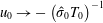$u_{0}\rightarrow -\left(\hat{\unicode[STIX]{x1D70E}}_{0}T_{0}\right)^{-1}$ as $\unicode[STIX]{x1D702}\rightarrow 0$ . Substituting (3.62) into the ${\mathcal{X}}$ (2.10) and balancing the convection and the diffusion terms in the limit $\unicode[STIX]{x1D702}\rightarrow 0$ , the new $O(1)$ wall-normal scaling variable, proportional to the $\text{VS}$ thickness, becomes

(3.73) $$\begin{eqnarray}\unicode[STIX]{x1D701}_{\text{III}}=G^{1/6}\hat{B}^{-1}\hat{x}^{1/3}\unicode[STIX]{x1D702},\end{eqnarray}$$

where $\hat{B}(\hat{x})\equiv [\unicode[STIX]{x1D707}_{0}/(2\unicode[STIX]{x1D706}\hat{\unicode[STIX]{x1D70E}}_{0}T_{0})]^{1/3}$ . A comparison with (3.29) shows that, by fixing $G$ and $\hat{B}$ , if $\hat{x}$ increases the $\text{VS}$ becomes thinner more rapidly in stage II $(O(\hat{x}^{-5/12}))$ than in stage III $(O(\hat{x}^{-1/3}))$ since $\unicode[STIX]{x1D701}_{II}$ and $\unicode[STIX]{x1D701}_{\text{III}}$ are of order one. The value of $\hat{B}(\hat{x})$ approaches a constant for $\hat{x}>5$ . From (3.73) it can be noticed that, in order to maintain $\unicode[STIX]{x1D701}_{\text{III}}=O(1)$ , $\unicode[STIX]{x1D702}$ must increase when $G$ increases, i.e. the $\text{VS}$ thickness is larger for flows over strong curvature. Substituting (3.62) into the LUBR equations (2.9)–(2.13) and balancing the convection and diffusion terms gives the expansion of the flow in the $\text{VS}$ ,

(3.74) $$\begin{eqnarray}\bar{\boldsymbol{q}}=\{G^{-1/2}u_{b},G^{-1/6}\hat{B}\hat{x}^{-1/3}v_{b},w_{b},G^{-2/3}\hat{B}\hat{x}^{-1/3}p_{b},G^{-1/2}\unicode[STIX]{x1D70F}_{b}\}\text{e}^{G^{1/2}\int ^{\hat{x}}\hat{\unicode[STIX]{x1D70E}}(x)\,\text{d}x},\end{eqnarray}$$

where $\bar{\boldsymbol{q}}(\hat{x},\unicode[STIX]{x1D701}_{\text{III}})=\{\bar{u},\bar{v},\bar{w},\bar{p},\bar{\unicode[STIX]{x1D70F}}\}(\hat{x},\unicode[STIX]{x1D701}_{\text{III}})$ . By substituting (3.74) into the LUBR equations (2.9)–(2.13), we recover the system of equations for $\hat{x}=O(1)$ and $\unicode[STIX]{x1D702}\rightarrow 0$ ,

(3.75) $$\begin{eqnarray}\displaystyle & \displaystyle {\mathcal{C}}\!\rceil \;\hat{\unicode[STIX]{x1D70E}}_{0}u_{b}+\frac{1}{T_{0}}v_{b}^{\prime }+w_{b}=0, & \displaystyle\end{eqnarray}$$

(3.76) $$\begin{eqnarray}\displaystyle & \displaystyle {\mathcal{X}}|\;\hat{\unicode[STIX]{x1D70E}}_{0}(\unicode[STIX]{x1D701}_{\text{III}}u_{b}-u_{b}^{\prime \prime })+\frac{1}{T_{0}}v_{b}=0, & \displaystyle\end{eqnarray}$$

(3.77) $$\begin{eqnarray}\displaystyle & \displaystyle {\mathcal{Y}}|\;p_{b}^{\prime }=0, & \displaystyle\end{eqnarray}$$

(3.78) $$\begin{eqnarray}\displaystyle & \displaystyle {\mathcal{Z}}|\;\unicode[STIX]{x1D706}\hat{\unicode[STIX]{x1D70E}}_{0}(\unicode[STIX]{x1D701}_{\text{III}}w_{b}-w_{b}^{\prime \prime })-k_{z}^{2}T_{0}p_{b}=0, & \displaystyle\end{eqnarray}$$

(3.79) $$\begin{eqnarray}\displaystyle & \displaystyle {\mathcal{E}}\!\rfloor \;\unicode[STIX]{x1D70F}_{b}^{\prime }=0, & \displaystyle\end{eqnarray}$$

where the prime $^{\prime }$ indicates the derivative with respect to $\unicode[STIX]{x1D701}_{\text{III}}$ . The equations are similar to the asymptotic eigensolution equations (3.31)–(3.35) and therefore $v_{b}$ satisfies the Airy equation (3.36) along with the boundary conditions (3.37) and (3.38). A composite solution for the streamwise velocity $u_{c}$ can be constructed from the solution in the $\text{ML}$ and $\text{VS}$ , i.e.  $u_{0}$ and $u_{b}$ , respectively, as

(3.80) $$\begin{eqnarray}u_{c}=u_{0}+u_{b}-u_{com},\end{eqnarray}$$

where

(3.81) $$\begin{eqnarray}u_{com}=\lim _{\unicode[STIX]{x1D702}\rightarrow 0}u_{0}=\lim _{\unicode[STIX]{x1D701}_{\text{III}}\rightarrow \infty }u_{b}=-\frac{1}{\hat{\unicode[STIX]{x1D70E}}_{0}T_{0}}\end{eqnarray}$$

is the common solution.

The streamwise velocity $u_{b}$ is computed by integrating (3.76) through the method of variation of parameters with the known velocity $v_{b}$ as the forcing term. The solution is

(3.82) $$\begin{eqnarray}u_{b}(\unicode[STIX]{x1D701}_{\text{III}})=C_{1}\text{Ai}+C_{2}\text{Bi}-\text{Ai}\int _{0}^{\unicode[STIX]{x1D701}_{\text{III}}}\frac{\text{f}\text{Bi}}{W}\,\text{d}\bar{\unicode[STIX]{x1D701}}_{\text{III}}+\text{Bi}\int _{0}^{\unicode[STIX]{x1D701}_{\text{III}}}\frac{\text{f}\text{Ai}}{W}\,\text{d}\bar{\unicode[STIX]{x1D701}}_{\text{III}},\end{eqnarray}$$

where $\text{Ai}=\text{Ai}(\unicode[STIX]{x1D701}_{\text{III}})$ and $\text{Bi}=\text{Bi}(\unicode[STIX]{x1D701}_{\text{III}})$ are the two linearly independent solutions of the Airy equation, $\text{f}(\unicode[STIX]{x1D701}_{\text{III}})=v_{b}(\unicode[STIX]{x1D701}_{\text{III}})/(\hat{\unicode[STIX]{x1D70E}}_{0}T_{0})$ and $W(\unicode[STIX]{x1D701}_{\text{III}})=\text{Ai}\,\text{Bi}^{\prime }-\text{Bi}\,\text{Ai}^{\prime }$ is the Wronskian. The constant $C_{2}=-0.2061$ is found first by numerically imposing the outer boundary condition (3.81) as the term proportional to $C_{1}$ vanishes as $\unicode[STIX]{x1D701}_{\text{III}}\rightarrow \infty$ . Once $C_{2}$ is known, the constant $C_{1}=0.3571$ is found by imposing the first of (3.37). The resulting solutions $\bar{u}_{b}$ , $\bar{u}_{0}$ , and $\bar{u}_{c}$ for $M=0.5$ and $M=3$ are displayed in figure 4. These results confirm that as the Mach number increases, but still remaining an order-one quantity, the vortices tend to move towards the wall when $G\gg 1$ . The requirement of a very high $G$ value in figure 4 arises from the inner coordinate being proportional to $G^{1/6}$ in (3.73) and is necessary to guarantee that the $\text{VS}$ is thinner than the $\text{ML}$ . The composite solution follows the inner $\text{VS}$ solution near the wall and the outer $\text{ML}$ solution away from the wall.

Figure 4.

Normalized profiles of the streamwise velocity perturbation for $M=0.5$ (a) and $M=3$ (b) from the eigensolution of stage III at $G=10^{15}$ and $\hat{x}=1$ . Insets: details of the solutions near the wall.

The viscous correction for $\hat{x}=O(1)$ and $\unicode[STIX]{x1D702}=O(1)$ is found by substituting the expansion (3.62) into the LUBR equations (2.9)–(2.13) and collecting the $O\left(G^{-1/6}\right)$ terms for $u_{1},v_{1},w_{1},p_{1},\unicode[STIX]{x1D70F}_{1}$ in (3.62),

(3.83) $$\begin{eqnarray}\displaystyle & \displaystyle {\mathcal{C}}\!\rceil \;\hat{\unicode[STIX]{x1D70E}}_{0}u_{1}-\frac{T^{\prime }}{T^{2}}v_{1}+\frac{1}{T}\frac{\unicode[STIX]{x2202}v_{1}}{\unicode[STIX]{x2202}\unicode[STIX]{x1D702}}+w_{1}-\hat{\unicode[STIX]{x1D70E}}_{0}\frac{F^{\prime }}{T}\unicode[STIX]{x1D70F}_{1}-\hat{\unicode[STIX]{x1D70E}}_{1}\frac{F^{\prime }}{T}\unicode[STIX]{x1D70F}_{0}+\hat{\unicode[STIX]{x1D70E}}_{1}u_{0}=0, & \displaystyle\end{eqnarray}$$

(3.84) $$\begin{eqnarray}\displaystyle & \displaystyle {\mathcal{X}}|\;\hat{\unicode[STIX]{x1D70E}}_{0}F^{\prime }u_{1}+\frac{F^{\prime \prime }}{T}v_{1}+\hat{\unicode[STIX]{x1D70E}}_{1}F^{\prime }u_{0}=0, & \displaystyle\end{eqnarray}$$

(3.85) $$\begin{eqnarray}\displaystyle & \displaystyle {\mathcal{Y}}|\;\frac{2F^{\prime }}{(2\hat{x})^{1/2}}u_{1}+\hat{\unicode[STIX]{x1D70E}}_{0}F^{\prime }v_{1}+\frac{1}{2\hat{x}}\frac{\unicode[STIX]{x2202}p_{1}}{\unicode[STIX]{x2202}\unicode[STIX]{x1D702}}-\frac{{F^{\prime }}^{2}}{(2\hat{x})^{1/2}T}\unicode[STIX]{x1D70F}_{1}+\hat{\unicode[STIX]{x1D70E}}_{1}F^{\prime }v_{0}=0, & \displaystyle\end{eqnarray}$$

(3.86) $$\begin{eqnarray}\displaystyle & \displaystyle {\mathcal{Z}}|\;\hat{\unicode[STIX]{x1D70E}}_{0}F^{\prime }w_{1}-k_{z}^{2}Tp_{1}+\hat{\unicode[STIX]{x1D70E}}_{1}F^{\prime }w_{0}=0, & \displaystyle\end{eqnarray}$$

(3.87) $$\begin{eqnarray}\displaystyle & \displaystyle {\mathcal{E}}\!\rfloor \;\frac{T^{\prime }}{T}v_{1}+\hat{\unicode[STIX]{x1D70E}}_{0}F^{\prime }\unicode[STIX]{x1D70F}_{1}+\hat{\unicode[STIX]{x1D70E}}_{1}F^{\prime }\unicode[STIX]{x1D70F}_{0}=0, & \displaystyle\end{eqnarray}$$

from which the equation for $v_{1}$ is derived

(3.88) $$\begin{eqnarray}\displaystyle & & \displaystyle \frac{\unicode[STIX]{x2202}^{2}v_{1}}{\unicode[STIX]{x2202}\unicode[STIX]{x1D702}^{2}}-2\frac{T^{\prime }}{T}\frac{\unicode[STIX]{x2202}v_{1}}{\unicode[STIX]{x2202}\unicode[STIX]{x1D702}}+\left[2\frac{F^{\prime \prime }T^{\prime }}{F^{\prime }T}-\frac{F^{\prime \prime \prime }}{F^{\prime }}-2\hat{x}k_{z}^{2}T^{2}+\frac{2(2\hat{x})^{1/2}k_{z}^{2}}{\hat{\unicode[STIX]{x1D70E}}_{0}^{2}}\frac{F^{\prime \prime }T}{F^{\prime }}-\frac{(2\hat{x})^{1/2}k_{z}^{2}}{\hat{\unicode[STIX]{x1D70E}}_{0}^{2}}T^{\prime }\right]v_{1}\nonumber\\ \displaystyle & & \displaystyle \quad =\frac{2(2\hat{x})^{1/2}k_{z}^{2}\hat{\unicode[STIX]{x1D70E}}_{1}}{\hat{\unicode[STIX]{x1D70E}}_{0}^{3}}\left(2\frac{F^{\prime \prime }T}{F^{\prime }}-T^{\prime }\right)v_{0},\end{eqnarray}$$

along with its boundary conditions

(3.89) $$\begin{eqnarray}\displaystyle & \displaystyle \unicode[STIX]{x1D702}=0\!\rceil \;v_{1}=\hat{B}\hat{x}^{-1/3}v_{\infty }, & \displaystyle\end{eqnarray}$$

(3.90) $$\begin{eqnarray}\displaystyle & \displaystyle \unicode[STIX]{x1D702}\rightarrow \infty \!\rfloor \;\frac{\unicode[STIX]{x2202}v_{1}}{\unicode[STIX]{x2202}\unicode[STIX]{x1D702}}\rightarrow 0. & \displaystyle\end{eqnarray}$$

As for the asymptotic eigensolution regime, the boundary condition for $\unicode[STIX]{x1D702}\rightarrow 0$ stems from the matching with the $\text{ML}$ solution. Applying the solvability condition to (3.88) gives

(3.91) $$\begin{eqnarray}\displaystyle & & \displaystyle \left(1+2\int _{0}^{\infty }\frac{T^{\prime }}{T}\frac{\unicode[STIX]{x2202}v_{0}}{\unicode[STIX]{x2202}\unicode[STIX]{x1D702}}\,\text{d}\unicode[STIX]{x1D702}\right)\left(\frac{2\unicode[STIX]{x1D706}\hat{\unicode[STIX]{x1D70E}}_{0}T}{\unicode[STIX]{x1D707}}\right)^{-1/3}\hat{x}^{-1/3}v_{\infty }\nonumber\\ \displaystyle & & \displaystyle \quad =-\frac{2(2\hat{x})^{1/2}k_{z}^{2}\hat{\unicode[STIX]{x1D70E}}_{1}}{\hat{\unicode[STIX]{x1D70E}}_{0}^{3}}\left(\int _{0}^{\infty }T^{\prime }v_{0}^{2}\,\text{d}\unicode[STIX]{x1D702}-2\int _{0}^{\infty }\frac{F^{\prime \prime }T}{F^{\prime }}v_{0}^{2}\,\text{d}\unicode[STIX]{x1D702}-2\int _{0}^{\infty }\frac{F^{\prime \prime }T}{F^{\prime }}v_{0}^{2}\,\text{d}\unicode[STIX]{x1D702}\right).\qquad\end{eqnarray}$$

The eigenvalue $\hat{\unicode[STIX]{x1D70E}}_{1}$ can either be calculated from the solvability condition or from the numerical integration of (3.88).

3.4 Stage IV. Wall layer regime: $\hat{x}\gg 1$

It has been shown by Hall (Reference Hall1983) and Wu et al. (Reference Wu, Zhao and Luo2011) for the incompressible case that, contrary to the Klebanoff modes generated over flat plates, Görtler vortices move towards the surface as they develop downstream in the limit $\hat{x}\gg 1$ ( $\unicode[STIX]{x1D6FF}^{\ast }\gg \unicode[STIX]{x1D706}_{z}^{\ast }$ ). It will be shown in § 4 that this is true only up to $M\simeq 3$ . For $M\geqslant 3$ , the perturbation initially tends to concentrate near the wall, but then, as $\hat{x}$ increases, it moves to the core of the boundary layer. Following the work of Wu et al. (Reference Wu, Zhao and Luo2011), the eigenvalue problem for the inviscid regime (3.69) can be simplified in the limit $\hat{x}\gg 1$ and $\unicode[STIX]{x1D702}\rightarrow 0$ . From the simplifications of the mean flow near the wall and introducing a new $\text{WL}$ variable $\hat{\unicode[STIX]{x1D701}}_{\text{III}}=(2\hat{x})^{1/2}\unicode[STIX]{x1D702}T_{0}$ to cancel the dependence on $\hat{x}$ , (3.69) simplifies to

(3.92) $$\begin{eqnarray}\frac{\unicode[STIX]{x2202}^{2}v_{0}}{\unicode[STIX]{x2202}\hat{\unicode[STIX]{x1D701}}_{\text{III}}^{2}}-\left(1-\frac{2}{\hat{\unicode[STIX]{x1D701}}_{\text{III}}\hat{\unicode[STIX]{x1D70E}}_{0}^{2}}\right)k_{z}^{2}v_{0}=0.\end{eqnarray}$$

This equation is the same as for the incompressible case and has a set of eigenvalues $\hat{\unicode[STIX]{x1D70E}}_{0}=(k_{z}/n)^{1/2}$ , with $n=1,2,3,\cdots \,$ (Denier, Hall & Seddougui Reference Denier, Hall and Seddougui1991). Applying the same procedure to (3.88), we find that $\hat{\unicode[STIX]{x1D70E}}_{1}=O(\hat{x}^{1/6})$ for $\hat{x}\gg 1$ and $\unicode[STIX]{x1D702}\rightarrow 0$ , which implies that, referring to (3.63), the viscous correction terms for the growth rate at $\unicode[STIX]{x1D702}=O(1)$ become of leading order as the flow evolves to $\hat{x}=O(G)$ .

For $\hat{x}\gg 1$ , we investigate the flow at $\hat{x}=O(G)$ , where the viscous correction term becomes of leading order. The streamwise and wall-normal variables rescale as

(3.93a,b ) $$\begin{eqnarray}\tilde{x}=\frac{\hat{x}}{G},\quad \unicode[STIX]{x1D701}_{\text{IV}}=(2\tilde{x})^{1/2}\unicode[STIX]{x1D702}G^{1/2}T_{0},\end{eqnarray}$$

respectively. From an order of magnitude analysis of the LUBR equations (2.9)–(2.13) the flow expands as

(3.94) $$\begin{eqnarray}\bar{\boldsymbol{q}}=\{\tilde{u} _{0},\tilde{v}_{0},G^{1/2}\tilde{w}_{0},G^{1/2}\tilde{p}_{0},G^{1/2}\tilde{\unicode[STIX]{x1D70F}}_{0}\}\text{e}^{G^{3/2}\int ^{\tilde{x}}\hat{\unicode[STIX]{x1D70E}}(x)\,\text{d}x},\end{eqnarray}$$

where $\bar{\boldsymbol{q}}(\tilde{x},\unicode[STIX]{x1D701}_{\text{IV}})=\{\bar{u},\bar{v},\bar{w},\bar{p},\bar{\unicode[STIX]{x1D70F}}\}(\tilde{x},\unicode[STIX]{x1D701}_{\text{IV}})$ . Substituting (3.94) into the LUBR equations (2.9)–(2.13) and using the near-wall approximations for the mean flow, the system of equations for $\hat{x}=O(G)$ becomes

(3.95) $$\begin{eqnarray}\displaystyle & \displaystyle {\mathcal{C}}\!\rceil \;\hat{\unicode[STIX]{x1D70E}}\tilde{u} _{0}+(2\tilde{x})^{1/2}\frac{\unicode[STIX]{x2202}\tilde{v}_{0}}{\unicode[STIX]{x2202}\unicode[STIX]{x1D701}_{\text{IV}}}+\tilde{w}_{0}+\left[\frac{\text{i}k_{x}R}{T}-\frac{\unicode[STIX]{x1D706}\unicode[STIX]{x1D701}_{\text{IV}}\hat{\unicode[STIX]{x1D70E}}}{\left(2\tilde{x}\right)^{1/2}T^{2}}\right]\tilde{\unicode[STIX]{x1D70F}}_{0}=0, & \displaystyle\end{eqnarray}$$

(3.96) $$\begin{eqnarray}\displaystyle & \displaystyle {\mathcal{X}}|\;\left[-\text{i}k_{x}R+\frac{\unicode[STIX]{x1D701}_{\text{IV}}\hat{\unicode[STIX]{x1D70E}}}{(2\tilde{x})^{1/2}}\frac{\unicode[STIX]{x1D706}}{T}+k_{z}^{2}\unicode[STIX]{x1D707}T\right]\tilde{u} _{0}-\unicode[STIX]{x1D707}T\frac{\unicode[STIX]{x2202}^{2}\tilde{u} _{0}}{\unicode[STIX]{x2202}\unicode[STIX]{x1D701}_{\text{IV}}^{2}}+\frac{\unicode[STIX]{x1D706}}{T}\tilde{v}_{0}-\frac{\unicode[STIX]{x1D706}\unicode[STIX]{x1D707}^{\prime }}{(2\tilde{x})^{1/2}}\frac{\unicode[STIX]{x2202}\tilde{\unicode[STIX]{x1D70F}}_{0}}{\unicode[STIX]{x2202}\unicode[STIX]{x1D701}_{\text{IV}}}=0, & \displaystyle\end{eqnarray}$$

(3.97) $$\begin{eqnarray}\displaystyle & & \displaystyle {\mathcal{Y}}|\;\frac{\unicode[STIX]{x1D701}_{\text{IV}}}{\tilde{x}}\frac{\unicode[STIX]{x1D706}}{T}\tilde{u} _{0}+\left[\frac{\unicode[STIX]{x1D701}_{\text{IV}}\hat{\unicode[STIX]{x1D70E}}}{(2\tilde{x})^{1/2}}\frac{\unicode[STIX]{x1D706}}{T}-\text{i}k_{x}R+k_{z}^{2}\unicode[STIX]{x1D707}T\right]\tilde{v}_{0}-\unicode[STIX]{x1D707}T\frac{\unicode[STIX]{x2202}^{2}\tilde{v}_{0}}{\unicode[STIX]{x2202}\unicode[STIX]{x1D701}_{\text{IV}}^{2}}+\frac{T}{(2\tilde{x})^{1/2}}\frac{\unicode[STIX]{x2202}\tilde{p}_{0}}{\unicode[STIX]{x2202}\unicode[STIX]{x1D701}_{\text{IV}}}\nonumber\\ \displaystyle & & \displaystyle \quad -\,\left[\frac{(\unicode[STIX]{x1D701}_{\text{IV}}\unicode[STIX]{x1D706})^{2}}{(2\tilde{x})^{3/2}T}+\frac{\hat{\unicode[STIX]{x1D70E}}\unicode[STIX]{x1D707}^{\prime }\unicode[STIX]{x1D706}}{2\tilde{x}}+\frac{\unicode[STIX]{x1D701}_{\text{IV}}\hat{\unicode[STIX]{x1D70E}}\unicode[STIX]{x1D707}^{\prime }\unicode[STIX]{x1D706}}{(2\tilde{x})^{2}}+\frac{\hat{\unicode[STIX]{x1D70E}}\unicode[STIX]{x1D707}\unicode[STIX]{x1D706}}{6\tilde{x}T}\right]\tilde{\unicode[STIX]{x1D70F}}_{0}+\left[\frac{\text{i}k_{x}R\unicode[STIX]{x1D707}}{3(2\tilde{x})^{1/2}}+\frac{\unicode[STIX]{x1D701}_{\text{IV}}\hat{\unicode[STIX]{x1D70E}}\unicode[STIX]{x1D707}\unicode[STIX]{x1D706}}{6\tilde{x}T}\right]\frac{\unicode[STIX]{x2202}\tilde{\unicode[STIX]{x1D70F}}_{0}}{\unicode[STIX]{x2202}\unicode[STIX]{x1D701}_{\text{IV}}}=0,\nonumber\\ \displaystyle & & \displaystyle\end{eqnarray}$$

(3.98) $$\begin{eqnarray}\displaystyle & \displaystyle {\mathcal{Z}}|\;\left[\frac{\unicode[STIX]{x1D701}_{\text{IV}}\hat{\unicode[STIX]{x1D70E}}\unicode[STIX]{x1D706}}{(2\tilde{x})^{1/2}T}-\text{i}k_{x}R+k_{z}^{2}\unicode[STIX]{x1D707}T\right]\tilde{w}_{0}-\unicode[STIX]{x1D707}T\frac{\unicode[STIX]{x2202}^{2}\tilde{w}_{0}}{\unicode[STIX]{x2202}\unicode[STIX]{x1D701}_{\text{IV}}^{2}}-k_{z}^{2}T\tilde{p}_{0}=0, & \displaystyle\end{eqnarray}$$

(3.99) $$\begin{eqnarray}\displaystyle & \displaystyle {\mathcal{E}}\!\rfloor \;\left[\frac{k_{z}^{2}}{Pr}\unicode[STIX]{x1D707}T-\text{i}k_{x}R+\frac{\unicode[STIX]{x1D701}_{\text{IV}}\hat{\unicode[STIX]{x1D70E}}\unicode[STIX]{x1D706}}{\left(2\tilde{x}\right)^{1/2}T}\right]\tilde{\unicode[STIX]{x1D70F}}_{0}-\frac{\unicode[STIX]{x1D707}T^{2}}{Pr}\frac{\unicode[STIX]{x2202}^{2}\tilde{\unicode[STIX]{x1D70F}}_{0}}{\unicode[STIX]{x2202}\unicode[STIX]{x1D701}_{\text{IV}}^{2}}=0. & \displaystyle\end{eqnarray}$$

These equations could be rearranged to eliminate $\tilde{w}_{0}$ and $\tilde{v}_{0}$ . The boundary conditions are $\tilde{u} _{0}=\tilde{v}_{0}=\tilde{\unicode[STIX]{x1D70F}}_{0}=0$ for $\unicode[STIX]{x1D701}_{\text{IV}}=0$ and $\tilde{u} _{0}$ , $\tilde{v}_{0}$ , $\tilde{\unicode[STIX]{x1D70F}}_{0}\rightarrow 0$ for $\unicode[STIX]{x1D701}_{\text{IV}}\rightarrow \infty$ . Finally, for $\tilde{x}=O(1)$ and from the boundary-layer thickness $\unicode[STIX]{x1D6FF}^{\ast }=O((\unicode[STIX]{x1D708}_{\infty }x^{\ast }/U_{\infty }^{\ast })^{1/2})$ , we find that $\unicode[STIX]{x1D6FF}^{\ast }/\unicode[STIX]{x1D706}_{z}^{\ast }=O(G^{1/2})$ , identified by Denier et al. (Reference Denier, Hall and Seddougui1991) as the most unstable regime for incompressible Görtler flow.

3.5 Summary of physical results emerging from the asymptotic analysis

From the asymptotic analysis in the limit $G\gg 1$ , we can infer the following physical properties:

1. (i) as in the incompressible case, the unbalance between pressure and centrifugal forces triggers the Görtler instability at a streamwise location $\hat{x}=O(G^{-2/5})$ , i.e. when both the wall-normal and the spanwise pressure gradients are active in the wall-normal and spanwise momentum equations, respectively;

2. (ii) in stage II, i.e. where the boundary-layer equations describe the flow as the spanwise viscous diffusion effects are negligible, increasing the Mach number causes:

   1. (a) the boundary-layer perturbation to intensify, as shown by the eigenvalues in table 1;

   2. (b) the perturbation to shift away from the wall;

3. (iii) in stage III, i.e. further downstream where the flow is described by the boundary-region equations because the spanwise viscous diffusion and the spanwise pressure gradient are at work:

   1. (a) the growth rate decreases slightly downstream, as shown in figure 4;

   2. (b) increasing the Mach number has a stabilizing effect on the growth rate, which is more intense in supersonic flow conditions, as figure 4 shows;

   3. (c) for $M=O(1)$ , the vortices move towards the wall as the Mach number increases, as shown in figures 3 and 4;

   4. (d) we have obtained a composite asymptotic solution, whose near-wall part is fully viscous and adiabatic, while the part in the boundary-layer core is inviscid.

4.1 Unsteady boundary-region results

Using the LUBR equations, we investigate the dependence of the evolution of compressible Görtler vortices on four main parameters, i.e. the Mach number, the Görtler number, the ratio of the disturbance wavelengths in the free stream and the frequency. In order to obtain realistic results, this parametric analysis is based on wind tunnel data of compressible flows.

4.1.1 Effect of Mach number

The effect of the Mach number is investigated while keeping a constant unit Reynolds number $R_{u}^{\ast }=U_{\infty }^{\ast }/\unicode[STIX]{x1D708}_{\infty }^{\ast }$ . As the free-stream mean velocity $U_{\infty }^{\ast }$ changes, it directly affects both $M$ and $R_{u}^{\ast }$ , $p_{\infty }^{\ast }$ affects $R_{u}^{\ast }$ through $\unicode[STIX]{x1D708}_{\infty }^{\ast }$ , whereas $T_{\infty }^{\ast }$ modifies $M$ through the speed of sound $a_{\infty }^{\ast }=a_{\infty }^{\ast }(T_{\infty }^{\ast })$ and changes $R_{u}^{\ast }$ through $\unicode[STIX]{x1D708}_{\infty }^{\ast }$ . The Reynolds number $R_{u}^{\ast }$ is thus kept constant by selecting the correct combination of $U_{\infty }^{\ast }$ , $T_{\infty }^{\ast }$ and $p_{\infty }^{\ast }$ as the desired $M$ is achieved. Figure 5 shows the influence of the free-stream temperature and pressure on the subsonic Mach number (a) and the free-stream kinematic viscosity (b).

Figure 5.

Influence of pressure $p_{\infty }^{\ast }$ and temperature $T_{\infty }^{\ast }$ on the subsonic Mach number (a) and on the kinematic viscosity $\unicode[STIX]{x1D708}_{\infty }^{\ast }$ of air (b) for $R_{u}^{\ast }=13\times 10^{6}~\text{m}^{-1}$ . The points in the two graphs correspond to the same flow conditions.

This approach has been used in several wind tunnel studies. Laufer (Reference Laufer1954) conducted experiments in the supersonic wind tunnel of the Jet Propulsion Laboratory in the range $1.4<M<4$ , with $R_{u}^{\ast }=13.3\times 10^{6}~\text{m}^{-1}$ and a free stream dominated by vortical disturbances. No information on the pressure and temperature conditions was given in their article. Flechner, Jacobs & Whitcomb (Reference Flechner, Jacobs and Whitcomb1976) studied transitional boundary layers in the transonic tunnel at NASA Langley Research Center and maintained the stagnation temperature at $322~\text{K}$ . Three different Mach numbers $M=0.7,0.8,0.83$ were investigated through a change in the free-stream dynamic pressure while keeping $R_{u}^{\ast }=13.1\times 10^{6}~\text{m}^{-1}$ . This wind tunnel was equipped with a control system that allowed independent variation of the Mach number, stagnation pressure and temperature. We consider the cases of steady vortices (frequency $f^{\ast }=0$ ) in conditions similar to the experimental configuration of De Luca et al. (Reference De Luca, Cardone, Aymer de la Chevalerie and Fonteneau1993), i.e. with spanwise wavelength $\unicode[STIX]{x1D706}_{z}^{\ast }=8\times 10^{-3}~\text{m}$ , corresponding to $R=1273.2$ , and radius of curvature $r^{\ast }=10~\text{m}$ , corresponding to $G=206.4$ . The Mach number is limited to $M\leqslant 4$ to maintain valid the assumptions of ideal gas and constant Prandtl number. The dimensionless wall-normal coordinate $y_{99}\equiv y^{\ast }/\unicode[STIX]{x1D6FF}_{99}^{\ast }$ is used when comparing results at different Mach numbers.

The maximum along $y_{99}$ of the amplitude of the streamwise velocity perturbation $|\bar{u}(\hat{x})|_{max}\equiv \max _{y_{99}}|\bar{u}(\hat{x},y_{99})|$ as a function of $\hat{x}$ is shown in figure 6(a) for different Mach numbers. For $\hat{x}=O(1)$ , increasing $M$ decreases the growth rate, i.e. the kinematic Görtler vortices ( $G_{V}$ -vortices) become more stable, especially for supersonic flows. This confirms the asymptotic results for stage III. This is true only sufficiently downstream from the leading edge where the Görtler instability is fully developed and $\unicode[STIX]{x1D6FF}^{\ast }$ is comparable with $\unicode[STIX]{x1D706}_{z}^{\ast }$ . In the early stages of the streamwise velocity perturbation where instead the spanwise viscous diffusion is negligible, the effect of the Mach number is reversed as shown in the inset of figure 6(a). This confirms the theoretical results for stage II. The stabilizing effect of the Mach number when $\unicode[STIX]{x1D6FF}^{\ast }=O(\unicode[STIX]{x1D706}_{z}^{\ast })$ is in accordance with early studies utilizing linearized theories for the primary instability (Hammerlin Reference Hammerlin1961; Kobayashi & Kohama Reference Kobayashi and Kohama1977; El-Hady & Verma Reference El-Hady and Verma1983; Hall & Malik Reference Hall and Malik1989; Spall & Malik Reference Spall and Malik1989; Wadey Reference Wadey1992). The most unstable Görtler vortices are therefore incompressible. However, this is true only during the initial stages of the evolution as the recent experimental study by Wang et al. (Reference Wang, Wang and Zhao2018) showed that transition to turbulence is achieved more rapidly for compressible Görtler vortices compared to the slower transition of incompressible Görtler vortices because the secondary instability of nonlinearly evolving vortices is more intense in the compressible case.

Figure 6.

The effect of the Mach number on the maximum streamwise velocity perturbation (a) and the maximum temperature perturbation (b) for a steady flow at $R=1273.2$ , $G=206.4$ and $k_{y}=1$ .

In addition to $G_{V}$ -vortices, compressibility effects generate thermal Görtler vortices, hereinafter called $G_{T}$ -vortices. They originate due to the velocity–temperature coupling within the boundary layer even in the absence of free-stream temperature disturbances, similar to the thermal Klebanoff modes over a flat plate (Ricco & Wu Reference Ricco and Wu2007). Figure 6(b) reveals that the temperature perturbations also grow exponentially and are more stable sufficiently downstream, i.e. their growth rate decreases, as the Mach number increases. However, thanks to our receptivity framework we notice that in the proximity of the leading edge, where $\unicode[STIX]{x1D6FF}^{\ast }$ is smaller than $\unicode[STIX]{x1D706}_{z}^{\ast }$ , the temperature perturbations increase much more significantly with the Mach number than the velocity perturbations. We further note that the stabilizing effect of the Mach number occurs much further upstream for the $G_{V}$ -vortices than for the $G_{T}$ -vortices. Since further downstream the growth rate decreases with increasing Mach number, temperature perturbations for lower Mach number become dominant when $\hat{x}$ is sufficiently high. This reversed influence of compressibility caused by the growing presence of spanwise viscous diffusion along the streamwise direction was also detected on thermal Klebanoff in the presence of wall heat transfer (Ricco et al. Reference Ricco, Tran and Ye2009). None of the previous theoretical frameworks could trace the evolution of the velocity and the temperature perturbations from the leading edge and observe this effect of spanwise diffusion because local EV approaches were utilized without considering the influence of the base-flow receptivity to external disturbances on the evolution of the Görtler vortices.

The location of the maximum value of the perturbation amplitude is monitored to evince the wall-normal position of the Görtler vortices. Early studies by Kobayashi & Kohama (Reference Kobayashi and Kohama1977), El-Hady & Verma (Reference El-Hady and Verma1983) and Ren & Fu (Reference Ren and Fu2015) show that the vortices lift away from the wall as the Mach number increases, although through EV approaches they could not trace the evolution of the vortices from the leading edge because the external forcing due to the free-stream disturbances plays a crucial role there. This effect of compressibility on Görtler vortices was also noticed by Spall & Malik (Reference Spall and Malik1989), Hall & Fu (Reference Hall and Fu1989) and Wadey (Reference Wadey1992). Previous studies have shown that in the limit of large Mach number the vortices move into a logarithmic layer near the free stream. However, as we focus on $M=O(1)$ , this lifting effect of the Mach number is not intense enough and the vortices are confined in the core of the boundary layer. Thanks to our receptivity framework, we can follow the wall-normal location of the $G_{V}$ -vortices and the $G_{T}$ -vortices as they evolve from the leading edge. Figure 7 confirms that by increasing the Mach number the $G_{V}$ -vortices (a) and the $G_{T}$ -vortices (b) occur at larger wall-normal locations. The influence of Mach number is stronger on the $G_{V}$ -vortices than on the $G_{T}$ -vortices and the $G_{T}$ -vortices are positioned closer to the free stream than the $G_{V}$ -vortices. The increase of boundary-layer thickness $\unicode[STIX]{x1D6FF}_{99}^{\ast }$ with the Mach number is also shown in the inset of figure 7(b).

Figure 7.

The effect of the Mach number on the wall-normal location of $G_{V}$ -vortices (a) and $G_{T}$ -vortices (b) for a steady flow at $R=1273.2$ , $G=206.4$ and $k_{y}=1$ . Inset: boundary-layer thickness based on $\unicode[STIX]{x1D706}_{z}^{\ast }=8\times 10^{-3}~\text{m}$ .

As shown by Hall (Reference Hall1983) and Wu et al. (Reference Wu, Zhao and Luo2011), incompressible Görtler vortices move closer to the surface as they evolve downstream and they become confined in the wall layer region. This behaviour persists in the compressible regime as long as $M<3$ . For $M\geqslant 3$ the vortices are not confined near the wall but they evolve in the core of the boundary layer. The asymptotic results of stage III, based on the assumption $G\gg 1$ , cannot capture this behaviour because vortices tend to shift towards the wall as $G$ increases for any Mach number when $M=O(1)$ .

Figure 8 shows the streamwise velocity perturbation profiles (a) and the spanwise velocity perturbation profiles (b) for $M=2$ and $M=4$ . Both the streamwise and the spanwise velocity profiles show that the perturbations move towards the wall for $M=2$ and remain confined in the boundary-layer core for $M=4$ . For this higher Mach number, the velocity gradient at the wall tends to zero as $\hat{x}$ increases, generating a near-wall region where the flow is largely unperturbed. Consequently, for $M>3$ the wall shear stress of the perturbation is not a sound indicator for the growth of thermal Görtler vortices, while it is effective in the incompressible regime (Hall Reference Hall1983, Reference Hall1990). Temperature profiles behave similarly to the streamwise velocity profiles and their peak shifts slightly towards the free stream (not shown).

Figure 8.

Influence of the Mach number, $M=2$ (

) and $M=4$ (

), on the normalized profiles of the streamwise velocity perturbation (a) and the spanwise velocity perturbation (b) for a steady flow at $R=1273.2$ , $G=206.4$ and $k_{y}=1$ . Numbers in the parenthesis correspond to the streamwise location $\hat{x}$ .

Table 2.

Streamwise locations $\hat{x}_{\unicode[STIX]{x1D6FD}}$ for different values of the Görtler number and the Mach number for a steady flow with $R=1273.2$ and $k_{y}=1$ .

4.1.2 Effect of Görtler number

In the context of steady vortices, we now analyse the effect of the Görtler number on the evolution of perturbations for $M=2$ and $M=4$ . Keeping $R=1273.2$ , radii of curvature $r^{\ast }=5~\text{m}$ and $r^{\ast }=10~\text{m}$ give $G=412.8$ and $G=206.4$ , respectively.

The evolution of the perturbation is characterized by the parameter $\unicode[STIX]{x1D6FD}(\hat{x})\equiv \text{d}^{2}|\bar{u}(\hat{x})|_{max}/\text{d}\hat{x}^{2}$ (Viaro & Ricco Reference Viaro and Ricco2018). Klebanoff modes, for which $\unicode[STIX]{x1D6FD}<0$ due to their algebraic growth, first develop near the leading edge. When curvature effects become important the Klebanoff modes turn into Görtler vortices at a streamwise location $\hat{x}_{\unicode[STIX]{x1D6FD}}$ where $\unicode[STIX]{x1D6FD}=0$ and starts growing with $\unicode[STIX]{x1D6FD}>0$ . The effect of the Görtler and Mach numbers on $\hat{x}_{\unicode[STIX]{x1D6FD}}$ is shown in table 2. The location $\hat{x}_{\unicode[STIX]{x1D6FD}}$ decreases as the Görtler number increases for all the Mach numbers and for subsonic conditions there is no Mach number influence. For supersonic conditions and low enough Görtler number, $\hat{x}_{\unicode[STIX]{x1D6FD}}$ increases with the Mach number, but $\hat{x}_{\unicode[STIX]{x1D6FD}}$ becomes independent of the Mach number in supersonic conditions if the Görtler number is sufficiently large.

Klebanoff modes contribute to the initial growth of the perturbation and, for sufficiently small Görtler numbers, i.e.  $G<50$ for $M=4$ , they stabilize after a certain streamwise location, as shown in figure 9. Only when $G$ is large enough the instability is characterized by the more energetic Görtler vortices. This is confirmed by the recent experimental study of Wang et al. (Reference Wang, Wang and Zhao2018) where for low $G$ values only weak streaky structures are present and the centrifugal instability is detected only at higher Görtler numbers. Figure 9 also shows that, as the Görtler number increases, $G_{T}$ -vortices (b) are more unstable than $G_{V}$ -vortices (a) at $M=4$ .

Figure 9.

The effect of the Görtler number $G$ on the maximum streamwise velocity perturbation (a) and temperature perturbation (b) for a steady flow with $M=4$ , $R=1273.2$ and $k_{y}=1$ .

Figure 10.

The effect of the Görtler number $G$ on the wall-normal location of $G_{V}$ -vortices at $M=2$ (a) and $M=4$ (b) for a steady flow with $R=1273.2$ and $k_{y}=1$ .

The location of $G_{V}$ -vortices is shown in figure 10 for $M=2$ (a) and $M=4$ (b). When the Görtler number increases the vortices move closer to the wall whereas when the Mach number grows they move away from the wall. High-Mach-number flows tend to behave more similarly to the flat-plate scenario.

The influence of the Mach number changes as the Görtler number increases. The asymptotic analysis reveals that for $G\gg 1$ an increase of the Mach number makes the vortices move towards the wall. This was also noticed by Dando & Seddougui (Reference Dando and Seddougui1993) and it is confirmed by the LUBR results for high Görtler numbers. Table 3 schematically shows that, when $\hat{x}$ is held fixed and the subsonic or mildly supersonic Mach number increases, the vortices shift towards the boundary-layer core only when $G=O(1)$ . In addition, the position of the vortices as $\hat{x}$ increases is affected by the Mach number being smaller or larger than 3 for $G=O(1)$ , as shown in figure 7.

Table 3.

Influence of $G$ , $M$ and $\hat{x}$ on the location of the Görtler vortices. Upward arrows ( $\uparrow$ ) indicate increasing values and horizontal arrows ( $\rightarrow$ ) denote the vortices moving towards the wall or the boundary-layer core.

Figure 11(a,b) shows the streamwise velocity and temperature perturbation profiles at different streamwise locations. These profiles highlight the unperturbed near-wall regions for $M=4$ caused by the $G_{V}$ -vortices and the $G_{T}$ -vortices moving towards the free stream. The peaks in the profiles experience only a minor shift towards the wall as the Görtler number increases due to the high Mach number. Like for the Mach-number effects, the influence of the Görtler number increases as the solution evolves downstream. The wall-normal velocity perturbation and the spanwise velocity perturbation represent the weak cross-flow of the Görtler instability. These profiles, shown in figure 11(c,d) for different values of $G$ , demonstrate that even though the free-stream vortical disturbance decreases exponentially in the streamwise direction, as described by (2.16) and (2.17), the perturbations inside the boundary layer soon become self-sustained when curvature effects become significant. The wall-normal velocity profiles present a single peak at $\unicode[STIX]{x1D702}\approx 2$ whereas the spanwise velocity profiles, which are more affected by $G$ , show the double-peak characteristic of the longitudinal counter-rotating $G_{V}$ -vortices. As in the case of the streamwise perturbation velocity, the solution for $\hat{x}=0.06$ differs only slightly from the flat-plate one, proving that the influence of curvature is still weak. The confinement of the $G_{V}$ -vortices in the core of the boundary layer is also visible from the cross-flow velocity profiles of figure 11(c,d).

Figure 11.

The effect of the Görtler number $G$ , $G=0$ (

), $G=206.4$ (

) and $G=412.8$ (

), on the normalized profiles of the streamwise velocity perturbation (a), the temperature perturbation (b), the wall-normal velocity perturbation (c) and the spanwise velocity perturbation (d) for a steady flow at $R=1273.2$ , $M=4$ and $k_{y}=1$ . Numbers in the parenthesis correspond to the streamwise location $\hat{x}$ .

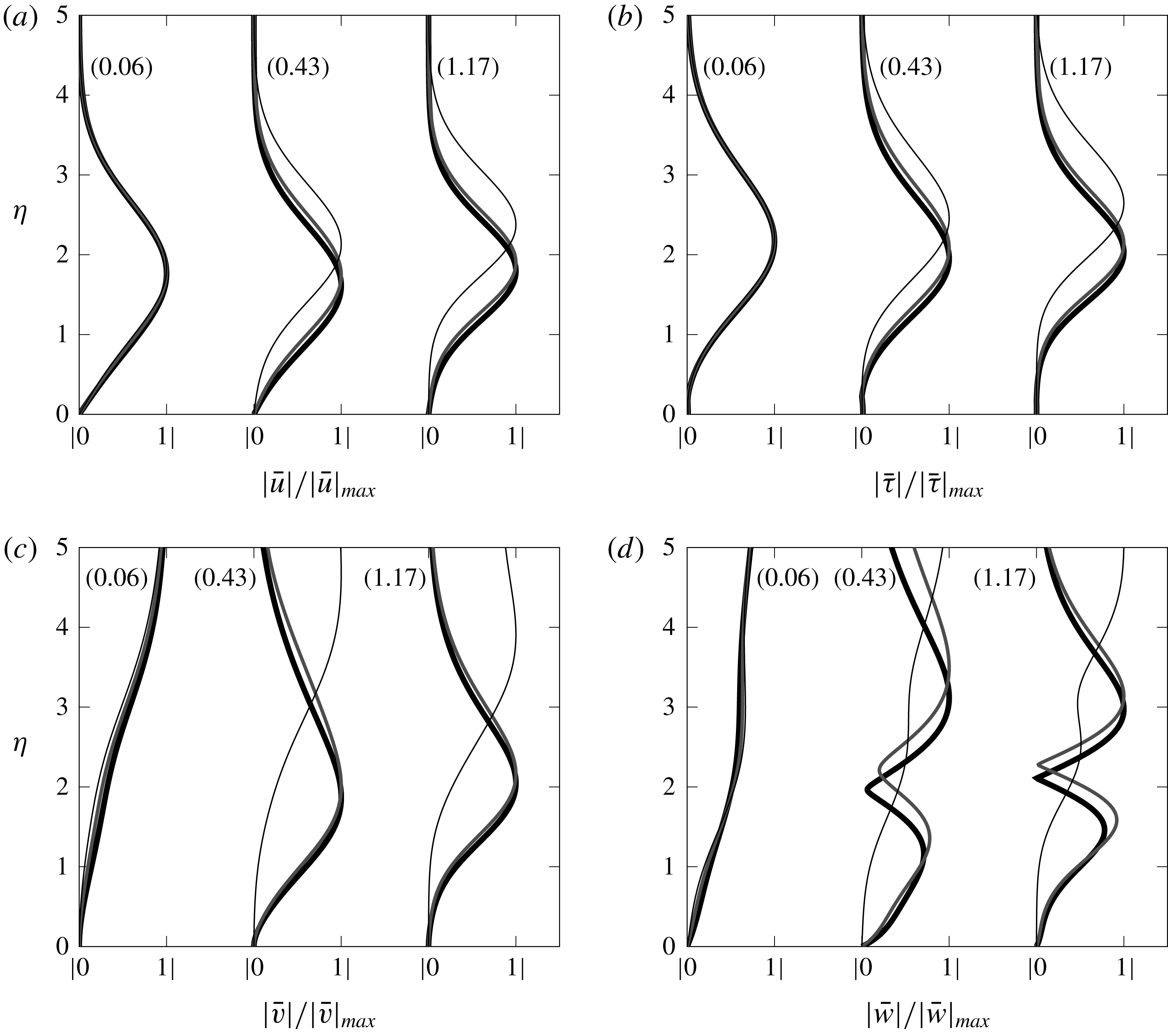
Previous studies have investigated how changes of the Görtler number affect the solution as the Mach number increases. The EV approach of El-Hady & Verma (Reference El-Hady and Verma1983) demonstrates that Görtler vortices are more sensitive to changes in the Görtler number as the Mach number grows. On the contrary, we show that Görtler vortices are less sensitive to changes in the curvature as the Mach number increases (e.g. refer to figure 10), which is in agreement with the results of Spall & Malik (Reference Spall and Malik1989).

4.1.3 Effect of free-stream wavelength ratio

The effect of the free-stream wavelength ratio $k_{y}=\unicode[STIX]{x1D706}_{z}^{\ast }/\unicode[STIX]{x1D706}_{y}^{\ast }$ can only be studied through the receptivity formalism because $k_{y}$ only appears in the initial and free-stream boundary conditions, i.e. equations (2.20)–(2.24) and (2.14)–(2.19), respectively. Figure 12 shows the effect of $k_{y}$ on the streamwise perturbation velocity (a) and the wall-normal location of the $G_{V}$ -vortices (b) for $M=4$ and $G=206.4$ . The weak effect of $k_{y}$ increases at higher Mach numbers (not shown). The flow becomes slightly more stable as $k_{y}$ increases, with the most unstable configuration achieved for $k_{y}=0$ . The growth rate of the streamwise velocity becomes nearly constant for sufficiently high $\hat{x}$ . When the flow is more stable as $k_{y}$ increases, the vortices initially tend to shift towards the wall but their wall-normal position becomes independent on $k_{y}$ at sufficiently high values of $\hat{x}$ , as shown in figure 12(b). Contrary to the effect of Mach number and Görtler number, the influence of $k_{y}$ on the wall-normal position of the vortices decreases as the streamwise location increases. Spall & Malik (Reference Spall and Malik1989) also noted that, for different initial conditions, the growth rates converged at sufficiently high scaled wavenumbers, i.e. sufficiently downstream, and that this convergence occurs closer to the leading edge as the Görtler number increases. The normalized streamwise velocity and the temperature profiles experience no significant variations as $k_{y}$ changes whereas the profiles of the cross-flow velocities vary with $k_{y}$ but only at small streamwise locations (not shown).

Figure 12.

The effect of $k_{y}$ on the maximum streamwise velocity perturbation (a) and wall-normal location of $G_{V}$ -vortices (b) for a steady flow at $R=1273.2$ , $G=206.4$ and $M=4$ .

4.1.4 Effect of frequency

The effect of frequency at two different Mach numbers, $M=0.5$ and $M=3$ , is investigated by keeping a constant dimensionless wavenumber $\unicode[STIX]{x1D705}=k_{z}/(k_{x}R)^{1/2}=O(1)$ that, for $\hat{x}=O(1)$ , is representative of the ratio $\unicode[STIX]{x1D6FF}^{\ast }/\unicode[STIX]{x1D706}_{z}^{\ast }=O(1)$ , i.e. the spanwise and the wall-normal diffusion effects are comparable. Flows at different Görtler numbers are also compared for $r^{\ast }=5~\text{m}$ and $r^{\ast }=10~\text{m}$ . For the subsonic case the Görtler numbers are $G=2494.7$ and $G=1247.3$ , whereas, for the supersonic case, $G=479.4$ and $G=239.7$ , respectively. The frequency is scaled as

(4.1) $$\begin{eqnarray}F\equiv \frac{f^{\ast }}{R_{u}^{\ast }U_{\infty }^{\ast }},\end{eqnarray}$$

where the unit Reynolds numbers are $R_{u}^{\ast }=11\times 10^{6}~\text{m}^{-1}$ and $R_{u}^{\ast }=2.18\times 10^{6}~\text{m}^{-1}$ for a subsonic case (Flechner et al. Reference Flechner, Jacobs and Whitcomb1976) and a supersonic case (Graziosi & Brown Reference Graziosi and Brown2002), respectively. For each Mach number, the effect of frequency is studied by doubling and halving a reference frequency from wind tunnel experiments for supersonic and subsonic flows. At $M=3$ , the reference frequency $f^{\ast }=1000~\text{Hz}$ ( $F=7.5\times 10^{-7}$ ) comes from the work of Graziosi & Brown (Reference Graziosi and Brown2002), which corresponds to the maximum perturbation energy. Given that no experiments were found for $M=0.5$ , the reference frequency $f^{\ast }=250~\text{Hz}$ ( $F=1.32\times 10^{-7}$ ) was inferred from the knowledge of frequencies at very low Mach numbers (Boiko et al. Reference Boiko, Ivanov, Kachanov and Mischenko2010b ), $f_{max}^{\ast }\approx 20~\text{Hz}$ , and at high Mach numbers (Graziosi & Brown Reference Graziosi and Brown2002), $f_{max}^{\ast }\approx 10~\text{kHz}$ . This value additionally allows us to compare the same frequency, $f^{\ast }=500~\text{Hz}$ , in the two Mach numbers considered. The parameters used to investigate the effect of frequency are summarized in table 4, along with the estimation of the boundary-layer displacement thickness $\unicode[STIX]{x1D6FF}_{c}^{\ast }=\unicode[STIX]{x1D6FF}_{i}^{\ast }+1.192(\unicode[STIX]{x1D6FE}-1)M^{2}x_{max}^{\ast }/R^{0.5}$ (Stewartson Reference Stewartson1964), where $\unicode[STIX]{x1D6FF}_{i}^{\ast }$ is the displacement thickness for incompressible flows and $x_{max}^{\ast }=2~\text{m}$ .

Figure 13.

The effect of the frequency $F$ on the maximum temperature perturbation for a plate with $r^{\ast }=5~\text{m}$ and $k_{y}=1$ , at $M=0.5$ , $G=2494.7$ (a) and $M=3$ , $G=479.4$ (b).

Table 4.

Flow parameters from wind tunnel data used for the analysis of the unsteady Görtler instability at $r^{\ast }=5~\text{m}$ and $r^{\ast }=10~\text{m}$ . Reference cases are in bold.

Figure 13 shows the stabilizing effect of increasing the frequency on the temperature perturbation while keeping a constant radius of curvature $r^{\ast }=5~\text{m}$ . The stabilizing influence of doubling the reference frequencies is more intense compared to the destabilizing effect of halving them, for both Mach numbers and for $r^{\ast }=10~\text{m}$ (not shown). The same conclusions can be drawn for the maximum velocity perturbation $|\bar{u}(\hat{x})|_{max}$ , which also agree with the findings of Hall (Reference Hall1990) and Ren & Fu (Reference Ren and Fu2015).

Frequency plays an important role on the location of Görtler vortices. As the main effect of increasing the frequency is to move the vortices away from the wall, figure 14(a) shows that, even for low Mach numbers, $G_{T}$ -vortices are not confined near the wall if the frequency is high enough. At high Mach numbers, the effect of frequency on the location of $G_{T}$ -vortices is more intense and starts closer to the leading edge, as shown in figure 14(b). $G_{V}$ -vortices are located closer to the wall with a weaker dependence on the frequency than $G_{T}$ -vortices (not shown).

To summarize, Görtler vortices tend to move towards the boundary-layer core when the perturbation is more stable, i.e. as $F$ or $M$ increase, or $G$ decreases. As $k_{y}$ increases, the perturbation is slightly more stable and Görtler vortices tend to move closer to the wall.

Figure 14.

The effect of the frequency $F$ on the wall-normal location of $G_{T}$ -vortices for a plate with $r^{\ast }=5~\text{m}$ and $k_{y}=1$ , at $M=0.5$ , $G=2494.7$ (a) and $M=3$ , $G=479.4$ (b).

4.1.5 Growth rate and streamwise length scale of the perturbation

From the solution of the LUBR equations, the streamwise velocity of the perturbation $\bar{u}=\bar{u}(\hat{x},\unicode[STIX]{x1D702})$ can be used to compute the complex parameter $\unicode[STIX]{x1D70E}=\unicode[STIX]{x1D70E}_{Re}+\text{i}\unicode[STIX]{x1D70E}_{Im}$ as

(4.2) $$\begin{eqnarray}\unicode[STIX]{x1D70E}(\hat{x},\unicode[STIX]{x1D702})=\left.\frac{1}{\bar{u}}\frac{\unicode[STIX]{x2202}\bar{u}}{\unicode[STIX]{x2202}\hat{x}}\right|_{\unicode[STIX]{x1D702}},\end{eqnarray}$$

where $\unicode[STIX]{x1D70E}_{Re}$ is the growth rate and $\unicode[STIX]{x1D70E}_{Im}$ is proportional to the inverse of the streamwise length scale. In the EV framework, applying the decomposition (2.25) to (4.2) gives $\unicode[STIX]{x1D70E}=\unicode[STIX]{x1D70E}_{EV}(\hat{x})$ . However, figure 15 shows that the perturbation inside the boundary layer grows at different rates at different wall-normal locations $\unicode[STIX]{x1D702}$ , with the maximum growth rate located at $\unicode[STIX]{x1D702}\approx 2$ . The dependence on $\unicode[STIX]{x1D702}$ is more intense closer to the leading edge and decreases at large $\hat{x}$ , but, even at large $\hat{x}$ this effect is still not negligible, especially in supersonic conditions. The relative difference $\unicode[STIX]{x0394}\unicode[STIX]{x1D70E}_{Re}$ between the maximum and minimum value of $\unicode[STIX]{x1D70E}_{Re}(\hat{x},\unicode[STIX]{x1D702})$ at $\hat{x}=10$ , i.e.  $\unicode[STIX]{x0394}\unicode[STIX]{x1D70E}_{Re}=(\unicode[STIX]{x1D70E}_{Re,max}-\unicode[STIX]{x1D70E}_{Re,min})/\unicode[STIX]{x1D70E}_{Re,max}$ , is $\unicode[STIX]{x0394}\unicode[STIX]{x1D70E}_{Re}=7.2\,\%$ and $\unicode[STIX]{x0394}\unicode[STIX]{x1D70E}_{Re}=29.9\,\%$ for $M=0.5$ and $M=3$ , respectively. This is confirmed by figure 15(b) where the perturbation closest to the wall displays the lowest growth rate.

Figure 15.

Influence of $\unicode[STIX]{x1D702}$ on $\unicode[STIX]{x1D70E}_{Re}(\hat{x},\unicode[STIX]{x1D702})$ for $M=0.5$ , $G=1247.3$ , $k_{y}=1$ , $F=1.32\times 10^{-7}$ (a) and $M=3$ , $G=239.7$ , $k_{y}=1$ , $F=7.5\times 10^{-7}$ (b).

The imaginary part of (4.2), $\unicode[STIX]{x1D70E}_{Im}(\hat{x},\unicode[STIX]{x1D702})$ , can be used to define the streamwise length scale of the boundary-layer perturbation as

(4.3) $$\begin{eqnarray}\unicode[STIX]{x1D706}_{x,bl}(x,\unicode[STIX]{x1D702})\equiv \frac{2\unicode[STIX]{x03C0}R}{\unicode[STIX]{x1D70E}_{Im}(\hat{x},\unicode[STIX]{x1D702})},\end{eqnarray}$$

which, as shown schematically in figure 1, is linked through receptivity to $\unicode[STIX]{x1D706}_{x}$ , the constant streamwise wavelength of the free-stream disturbance. The parameter

(4.4) $$\begin{eqnarray}{\mathcal{L}}_{x}(x,\unicode[STIX]{x1D702})\equiv \frac{\unicode[STIX]{x1D706}_{x,bl}}{\unicode[STIX]{x1D706}_{x}}=\frac{k_{x}R}{\unicode[STIX]{x1D70E}_{Im}(\hat{x},\unicode[STIX]{x1D702})}\end{eqnarray}$$

can therefore be defined. Figure 16 shows the dependence of ${\mathcal{L}}_{x}$ on $\unicode[STIX]{x1D702}$ for $M=0.5$ (a) and for $M=3$ (b). For all cases considered ${\mathcal{L}}_{x}<1$ , which means that the streamwise boundary-layer length scale is always smaller than the streamwise free-stream wavelength. The ratio decreases with $\hat{x}$ near the leading edge, but then increases as the perturbation evolves, i.e.  $\unicode[STIX]{x1D706}_{x,bl}$ approaches $\unicode[STIX]{x1D706}_{x}$ further downstream. As the Mach number increases ${\mathcal{L}}_{x}$ becomes closer to unity, as shown in figure 16(b). Increasing the frequency also has the same effect (not shown). Therefore, the more unstable the perturbation is, the more $\unicode[STIX]{x1D706}_{x,bl}$ differs from $\unicode[STIX]{x1D706}_{x}$ .

Figure 16.

Influence of $\unicode[STIX]{x1D702}$ on ${\mathcal{L}}_{x}(x,\unicode[STIX]{x1D702})$ for $M=0.5$ , $G=1247.3$ , $k_{y}=1$ , $F=1.32\times 10^{-7}$ (a) and $M=3$ , $G=239.7$ , $k_{y}=1$ , $F=7.5\times 10^{-7}$ (b).

4.2 Comparison with results from the eigenvalue analysis

We now compare the LUBR solution with the solutions of the parallel and non-parallel EV equations.

4.2.1 Growth rate and streamwise length scale of the boundary-layer perturbation

Figure 17 shows the comparison between the growth rate (a) and the streamwise length scale ratio (b) of the LUBR solution and EV solution. The most important point is that the receptivity process selects the most unstable modes, which, in the limit $G\gg 1$ , correspond to the first eigenvalues of table 1. The non-parallel EV solution (solid circles) is a better approximation for the growth rate and the streamwise length scale than the parallel EV solution (empty circles) at $\unicode[STIX]{x1D702}=2$ , where the growth rate is at its maximum. The parallel and non-parallel EV formulations show the strongest disagreement with the receptivity LUBR solution closer to the leading edge, where the solution has not yet acquired a modal form. In this region, the non-parallel effects and the initial and free-stream boundary conditions thus play a key role in the dynamics of the perturbation. In the limit $\hat{x}\rightarrow 0$ the EV solution is invalid, with the growth rate becoming negative. Results show a tendency of the EV approach to overestimate the growth rate, which is in agreement with the results of Spall & Malik (Reference Spall and Malik1989). The agreement between the LUBR solution and the parallel EV solution is worse in the supersonic case than in the subsonic case. The use of the rigorous receptivity LUBR framework becomes therefore essential to capture the entire evolution of the perturbations inside the boundary layer.

Figure 17.

Comparison between the LUBR $\unicode[STIX]{x1D70E}_{Re}(\hat{x},\unicode[STIX]{x1D702})$ (——) at $\unicode[STIX]{x1D702}=2$ , the non-parallel EV $\unicode[STIX]{x1D70E}_{EV,Re}(\hat{x})$ (●) and the parallel EV $\unicode[STIX]{x1D70E}_{EV,Re}(\hat{x})$ (○) (a) and comparison between the LUBR ${\mathcal{L}}_{x}(\hat{x},\unicode[STIX]{x1D702})$ (——) at $\unicode[STIX]{x1D702}=2$ , the non-parallel EV ${\mathcal{L}}_{x,EV}(\hat{x})$ (●) and the parallel EV ${\mathcal{L}}_{x,EV}(\hat{x})$ (○) (b), for $M=3$ , $G=1247.3$ , $k_{y}=1$ , $F=1.32\times 10^{-7}$ and $M=3$ , $G=239.7$ , $k_{y}=1$ , $F=7.5\times 10^{-7}$ .

4.2.2 Velocity and temperature profiles

The velocity and temperature EV profiles are compared with the LUBR profiles in figure 18 for $M=3$ . Since the eigenfunctions are obtained to within an arbitrary undefined constant, the solutions are normalized by the maximum values at each streamwise location to be compared with the LUBR solutions. The non-parallel EV solution approximates the profiles well for sufficiently high $\hat{x}$ . Under the parallel-flow approximation, the maximum of the perturbation is slightly shifted upwards and the solution is overestimated in the region above the maximum, especially near the leading edge, where the non-parallel effects are most significant. As the wall is approached both the parallel and the non-parallel EV solutions agree well with the LUBR solution.

Figure 18.

Comparison between the LUBR solution (

), the non-parallel EV solution (●) and the parallel EV solution (○) for the streamwise velocity profiles (a) and temperature profiles (b) at $M=3$ , $F=7.5\times 10^{-7}$ , $G=239.73$ , $k_{y}=1$ . Numbers in the parenthesis correspond to the streamwise location $\hat{x}$ .

The cross-flow profiles shown in figure 19 highlight the limit of the EV solution. Close to the leading edge there is a strong influence of the free-stream vortical disturbances that cannot be captured by the simplified EV framework. Therefore, a correct analysis in this region is only possible when the receptivity of the base flow to the external vortical disturbances is considered. The disagreement in the free stream is expected, but the solutions do not even match near the wall. The non-parallel EV solution begins to approximate the cross-flow perturbations well only for sufficiently high $\hat{x}$ . We previously demonstrated how the growth rate is not only a function of $\hat{x}$ , as shown by the decomposition (2.25), but it does also change with $\unicode[STIX]{x1D702}$ even at large streamwise locations. Similarly, figures 18 and 19 demonstrate that the eigensolutions are not a simple function of $\unicode[STIX]{x1D702}$ but do depend on the streamwise location $\hat{x}$ .

Figure 19.

Comparison between the LUBR solution (

), the non-parallel EV solution (●) and the parallel EV solution (○) for the wall-normal velocity profiles (a) and spanwise velocity profiles (b) at $M=3$ , $F=7.5\times 10^{-7}$ , $G=239.73$ , $k_{y}=1$ . Numbers in the parenthesis correspond to the streamwise location $\hat{x}$ .

4.3 Comparison with results from the asymptotic analysis

The asymptotic exponents $\breve{\unicode[STIX]{x1D70E}}(\breve{x})$ in (3.42) denote the earliest growth of the Görtler vortices triggered by the external free-stream disturbances. As the instability evolves, they turn into the fully developed local eigenmodes $\unicode[STIX]{x1D70E}_{EV}(\hat{x})$ of (2.25). From (3.62) the streamwise velocity of the stage III solution multiplied by $G^{-1/2}$ can be compared with the LUBR streamwise velocity $\bar{u}$ . Figure 20 shows that the growth rate (a) and the normalized streamwise velocity LUBR profiles (b) tend to the asymptotic solution as the Görtler number increases. This is in accordance with the $G\gg 1$ limit of the asymptotic analysis, although it occurs at very high Görtler and at high $\hat{x}$ .

Figure 20.

Comparison between the composite solution $\bar{u}_{c}$ from the asymptotic stage III for $G=10^{15}$ (– – –) and the LUBR results of the growth rates at $\unicode[STIX]{x1D702}=2$ (a) and of the normalized streamwise velocity profiles at $\hat{x}=1$ (b) for $M=3$ .

4.4 Qualitative comparison with DNS data

The lack of experimental data for compressible Görtler flows makes it difficult to validate our results. We here carry out a qualitative comparison with the DNS data by Whang & Zhong (Reference Whang and Zhong2003), who first studied the response of a hypersonic boundary layer ( $M=15$ ) over a concave surface to free-stream vortical and acoustic disturbances. As the Mach number in their simulations is much higher than ours, quantitative agreement with our moderate supersonic data would not be possible. Nevertheless, our receptivity analysis results are useful because they explain the physics of the instability observed by Whang & Zhong (Reference Whang and Zhong2003). In their work, the DNS data are compared with data from the linear eigenvalue stability theory. As we have shown, this latter approach cannot fully capture the physics of the vortices, especially near the leading edge, where the effect of the free-stream perturbation is crucial.

Figure 21 presents the evolution of the amplitude of the steady streamwise and temperature perturbations obtained by Whang & Zhong (Reference Whang and Zhong2003)(a) and by our LUBR simulations (b). Values are normalized by the first peak value of the streamwise velocity. The streamwise velocity perturbation and the temperature perturbation evolve in similar fashion, showing the initial algebraic growth due to the streaks, followed by viscous decay and by the Görtler instability downstream. These three phases have been reported by Viaro & Ricco (Reference Viaro and Ricco2018) to occur at sufficiently low Görtler number to detect a competing effect between the damping action of the viscous effects and the centrifugal instability. Consistently with our results on the effect of Mach number, the temperature perturbations become larger and larger than the velocity perturbations as the Mach number grows.

Whang & Zhong (Reference Whang and Zhong2003) refer to the first growing phase as an early transient growth due to leading-edge effects and correctly identify the Görtler vortices as responsible for the subsequent instability following the intermediate decay. They also point out that, according to the linear stability theory, the region near the leading edge should be stable and the growth of disturbances should be absent. All these observations match our theoretical predictions. Our eigenvalue analysis indeed predicts decay near the leading edge where instead the direct forcing from the free stream creates the transient growth. We can then describe the initial growth reported by Whang & Zhong (Reference Whang and Zhong2003) as the thermal and kinematic Klebanoff modes, which are always present from the leading edge at every Görtler number (Viaro & Ricco Reference Viaro and Ricco2018) and are caused by the free-stream receptivity, i.e. the continuous action of the free-stream vortical disturbances, and not only by a leading-edge effect as stated by Whang & Zhong (Reference Whang and Zhong2003).

Figure 21.

Comparison of velocity and temperature perturbations relative to the DNS data of Whang & Zhong (Reference Whang and Zhong2003) at $M=15$ (a) and the LUBR results at $M=4$ (b). Data are normalized by the peak of the perturbation velocity.

As we have shown, increasing the frequency has a stabilizing effect on the boundary-layer flow. This is consistent with the DNS results by Whang & Zhong (Reference Whang and Zhong2003), shown in figure 22(a) and compared with our LUBR results in figure 22(b). For sufficiently high frequency, the Klebanoff modes do not turn into Görtler vortices downstream. For the cases presented in figure 22 only steady perturbations are subject to centrifugal instability.

Figure 22.

Comparison of the influence of frequency relative to the DNS data of Whang & Zhong (Reference Whang and Zhong2003) at $M=15$ (a) and the LUBR results at $M=4$ (b). Data are normalized by the peak value for the steady case.