1. INTRODUCTION
Maritime transportation is a major aspect of the global economy; almost 90% of global trade volume and 70% of global trade value are conducted through the marine environment. It is also energy efficient – only 7% of all energy consumed by transportation activities is related to this mode of transportation (Rodrigue et al., Reference Rodrigue, Comtois and Slack2016). Therefore, increasing maritime safety and security is a paramount task. A study on marine collision reports revealed that 71% of human error is caused due to lack of situational awareness. Of such situational awareness errors, about 9% were related to the lack of awareness about future actions in the marine environment (Grech et al., Reference Grech, Horberry and Smith2002).
To enhance marine safety and security, since 2004 all vessels above a specific size have been obliged by the International Maritime Organization to be equipped with automatic identification systems (AISs) (SOLAS, 2003). AISs repeatedly broadcast both static and dynamic information. Static information contains marine mobile service identifier (MMSI), vessel name, type, and dimensions, whereas dynamic information includes latitude, longitude, speed over ground (SOG), and course over ground (COG) (Series, Reference Series2010). AIS messages are reported at different update rates, which vary according to vessel speed and status, and range from 2 s (while the vessel operates at high speed) to 3 min (while the vessel is anchored) (Harati-Mokhtari et al., Reference Harati-Mokhtari, Wall, Brooks and Wang2007). To enhance maritime situational awareness, various studies have been conducted using AIS data for detection of anomalous behaviour (Sidibé and Shu, Reference Sidibé and Shu2017; Zhao and Shi, Reference Zhao and Shi2019), extraction of shipping route patterns (Fujino et al., Reference Fujino, Claramunt and Boudraa2018; Sheng and Yin, Reference Sheng and Yin2018), prediction of vessel trajectory (Pallotta et al., Reference Pallotta, Vespe and Bryan2013; Wijaya and Nakamura, Reference Wijaya and Nakamura2013; Borkowski, Reference Borkowski2017; Duca et al., Reference Duca, Bacciu and Marchetti2017; Gao et al., Reference Gao, Shi and Li2018; Graser et al., Reference Graser, Schmidt and Widhalm2018; Mao et al., Reference Mao, Tu, Zhang, Rachmawati, Rajabally, Huang, Cao, Cambria, Lendasse, Miche and Vong2018), and traffic prediction (Xiao et al., Reference Xiao, Ponnambalam, Fu and Zhang2017; Kim and Lee, Reference Kim and Lee2018).
A necessary aspect of increasing maritime situational awareness is predicting target vessel trajectory effectively. In this regard, vessels should be able to predict the trajectories of other vessels which are located in their vicinity and adapt their movements to avoid any collision. Various models have been developed for predicting vessel trajectory so far. In general, the proposed models are either data-driven or model-driven. The model-driven models require that process parameters be estimated, which is not straightforward (Dalsnes et al., Reference Dalsnes, Hexeberg, Flåten, Eriksen and Brekke2018). Besides, these models become complicated and need more time when non-linearity of the movement increases (Kawan et al., Reference Kawan, Wang, Li and Chhantyal2017). Data-driven models not only address the drawbacks of model-driven models, but also predict vessel trajectory for longer durations, which is required in collision avoidance. However, data-driven models should be able to cope with a large amount of data (Graser et al., Reference Graser, Schmidt, Dragaschnig and Widhalm2019).
In this paper, vessel trajectory prediction is studied using the data-driven procedure. Predictions are carried out based on the assumption that vessels similar in pattern behaviour in the past will have similar patterns in the future. The sharp distinctions between this research and previous research are: (1) AIS messages are not considered individually, and the spatial correlation between AIS messages is taken into account. Therefore, the trajectory-based similarity is measured instead of point-based measure. (2) Distances between the target trajectory and the most similar trajectory are no longer considered constant during the prediction.
The structure of this paper is as follows. Section 2 provides an overview of the previous studies in vessel trajectory prediction. Section 3 introduces three prediction models. In Section 4, the proposed models are experimentally evaluated by preforming them on real AIS data sets, and the results are presented. Finally, Section 5 concludes the key remarks of the study and suggests promising research topics for future work.
2. RELATED WORK
Various models have been developed for trajectory prediction, which are generally classified as model-driven or data-driven approaches. The Gaussian mixture trajectory prediction (GMTP) model presented by Qiao et al. (Reference Qiao, Jin, Han, Tang and Gesangduoji2015) revealed the complex motion patterns based on Gaussian mixture models. They calculated the probability distribution of different types of motion patterns. The possible trajectories of input trajectory were then determined by Gaussian process regression. The results revealed that GMTP could improve prediction accuracy compared with the Gaussian process regression and the Kalman filter. Perera and Soares (Reference Perera and Soares2010) estimated ship position, velocity, and acceleration using an extended Kalman filter. Model-driven approaches require a mathematical model to be built for each trajectory, therefore they are not very suitable for dynamic environments (Tang et al., Reference Tang, Yin and Shen2019).
Data-driven approaches have made remarkable achievements in trajectory prediction. First, Gan et al. (Reference Gan, Liang, Li, Deng and Cheng2016) used the K-means algorithm to group AIS data. Secondly, the clusters achieved by the first step were used to train the artificial neural network (ANN) to predict the vessels' trajectories. The results showed a 70% prediction accuracy. Tang et al. (Reference Tang, Yin and Shen2019) constructed a neural network with two long short-term memory (LSTM) layers, which can observe the first 10 min of the vessel's state to predict the location of the vessel after 20 min. The experimental comparison revealed that the model performs better than the Kalman filter and backpropagation neural network. Nishizaki et al. (Reference Nishizaki, Terayama, Okazaki and Shoji2018) trained a support vector machine (SVM) to predict the next course of vessels that exited from the Nakanose traffic route, known as an exit point. They used the data related to the exit point, 5 min before the exit point, and 10 min before the exit point to train the SVM model. The result shows prediction accuracy of 87·9%, 80·3%, and 77% for the data related to exit point, 5 min, and 10 min before the exit point, respectively. However, the main drawback of their work was the disproportion of training data, which means the trained data mostly belonged to a particular class. Graser et al. (Reference Graser, Schmidt and Widhalm2018) applied three models – linear prediction, learned statistical, and similarity search – to vessel trajectories. The results proved that the similarity search approach performed accurately compared with the other two models for prediction. To predict the next location of the target point, Wijaya and Nakamura (Reference Wijaya and Nakamura2013) extracted the most similar points to the target point based on the assumption that spatial distances between the target point and the most similar point to it remain constant during the prediction. Long-term prediction is important in the maritime environment to gain sufficient time for the actions needed to control vessel movements (Kim and Lee, Reference Kim and Lee2018). However, previous works either carried out short-term prediction (Wijaya and Nakamura, Reference Wijaya and Nakamura2013; Graser et al., Reference Graser, Schmidt and Widhalm2018) or obtained unsatisfactory results in long-term prediction (Zorbas et al., Reference Zorbas, Zissis, Tserpes and Anagnostopoulos2015). To overcome these problems, three distinct models are proposed based on similarity searches that can predict vessels' trajectories for short and long durations.
3. METHODOLOGY
This section is dedicated to the pre-processing of raw AIS data and proposes three distinct models for predicting vessels' positions. All three models utilise similarity searches to predict the geographic location of a vessel at the moment ahead. The schematic diagram of the methodology presented in this work is illustrated in Figure 1.
Flow diagram of PSSP, TSSP, and TSSPL models.

3.1. Data pre-processing
Because of high redundancy in AIS data and complexity in extracting vessel movement patterns from raw AIS data, the data must be pre-processed. First, because only moving vessels are important, vessels with SOG values less than 1 knot, including anchored vessels, are eliminated from the data set. Second, to compose trajectories related to each vessel, the entries are grouped based on their MMSIs. In the next step, each unique trajectory is divided into individual trips, which are called voyages, if the gap observation between two consecutive AIS messages is greater than a time threshold ( $\varepsilon_{1}$). Finally, it is required that all records of each voyage be resampled into T min. The parameters of the minimum gap observation between two consecutive AIS records
 $( \varepsilon_{1}) $, bins for time resampling (T), minimum duration of each voyage
 $( \varepsilon_{2}) $, and minimum SOG
 $( \varepsilon_{3}) $ were set at 5 min, 10 min, 120 min, and 1 knot, respectively. As mentioned before, AIS messages are transmitted every 2 s to 3 min. Therefore, continuous trajectories have been split with gap observation
 $( \varepsilon_{1}) $ of 5 min.
3.2. Point-based similarity search prediction (PSSP)
To predict the next locations of the target vessels, the most similar vessel to the target vessel is considered. In the PSSP model, each AIS record is considered individually as a point and the distances between the last point of the target vessel (i.e., target point) and all the historical points are measured in terms of spatial, speed, and course variables. After extracting the most similar point to the target point from the historical points (i.e., the most similar extracted point), the next locations of the target vessel will be predicted using the most similar extracted point as follows. The main concept of this model has been inspired by Wijaya and Nakamura (Reference Wijaya and Nakamura2013); however, it has been modified here to increase the prediction accuracy.
3.2.1. Similarity measure phase
To measure how similar two points are in terms of spatial, speed, and course criteria, three similarity distance functions are defined.
Spatial similarity measure
The Haversine distance measures the spatial similarity of two points. It determines a great-circle distance between two points on a sphere using their latitudes and longitudes along the surface. As the Earth is nearly spherical, Haversine distance provides a good approximation for the shortest distance involving points over the Earth's surface, as is expressed by Equation (1) (Valsamis et al., Reference Valsamis, Tserpes, Zissis, Anagnostopoulos and Varvarigou2017). Smaller value of the calculated Haversine distance between two points indicates more spatial similarity.
 $$\begin{align} d_{d} &= 2r \ast {\sin ^{ - 1}}( \sin^{2}( {\dfrac{{\Delta \text{Latitude}}}{2}} ) + \cos({\text{Latitude}_{1}})\cdot \cos({\text{Latitude}_{2}}) \notag\\ &\quad \cdot \sin^{2}( {\dfrac{{\Delta \text{Longitude}}}{2}} ) ) \end{align}$$
where r is the radius of the Earth (6371 km). d d is the calculated Haversine distance between two points. Δ Latitude and Δ Longitude denote differences between the latitudes and longitudes of two points, respectively. Latitude1 shows the latitude of the first point, and Latitude2 is the latitude of the second point.
Speed similarity measure
To measure how similar two points are in terms of speed (SOG), the absolute difference of the speed of two points (d s) is calculated using Equation (2). The smaller the value of the absolute difference, the greater the similarity between two points is.
 $$d_s = \vert {\text{SOG}_1 - \text{SOG}_2 } \vert $$
where SOG1 and SOG2 denote the speeds of the first and second points, respectively.
Course similarity measure
To measure how similar two points are in terms of their course (COG), the absolute difference of the course of two points (d c) is calculated using Equation (3). The smaller the absolute difference, the greater the similarity between the two points is.
 $$d_c = \vert \hbox{COG}_1 - \text{COG}_2\vert $$
where COG1 and COG2 indicate the COG of the first and second points, respectively.
The values achieved from Equations (1)–(3) are normalised to the scale of 1 using the scikit-learn Python package due to the differences in their units of measurement. Finally, the most similar point to the target point in terms of spatial distance, speed, and course is determined using the overall weighted value of three similarity measure functions (Equation (4)).
 $$D_t = w_{d } \times d_d + w_{s } \times d_s + w_{c } \times d_c ,$$
where d d, d s, and d c stand for the normalised spatial, speed, and course similarity measures, respectively, and w d, w s, and w c are their corresponding weights. D t is the total similarity distance. The weight of each similarity measure criterion is determined based on the degree of its importance.
3.2.2. Location prediction phase
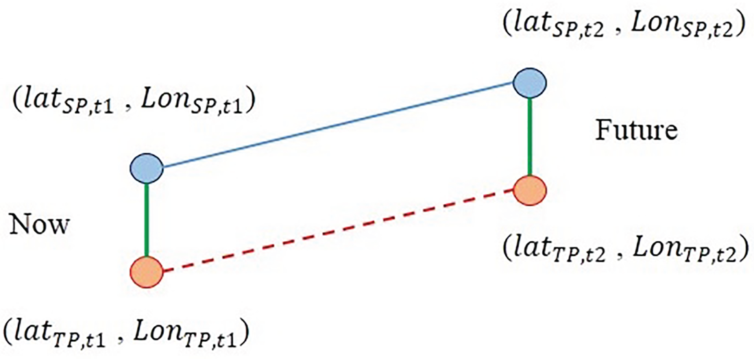
The most similar point extracted from historical data is used to predict the next location of the target point under the assumption that the spatial distances remain constant throughout the prediction. The schematic procedure of location prediction using PSSP is depicted in Figure 2.
The location prediction approach proposed in PSSP model.

In Figure 2,  $( {\text{Lat}_{\text{TP}.t1} , \; \text{Lon}_{\text{TP}. t1} } ) $ represents the coordinate of the target point at the current time and is known.
 $( {\text{Lat}_{\text{TP}.t2}, \; \text{Lon}_{\text{TP}. t2} } ) $ represents the coordinate of the target point at the future time, which is unknown and should be predicted. Likewise,
 $( {\text{Lat}_{\text{SP}. t1} , \; \text{Lon}_{\text{SP}. t1} }) $ and
 $( {\text{Lat}_{\text{SP}. t2}, \; \text{Lon}_{\text{SP}. t2} } ) $, which are both known, stand for coordinates of a similar point at the current and future times, respectively. The next location of the target point will be predicted using the most similar extracted point by Equations (5) and (6).
 $$\Delta \text{Longitude}=\text{Lon}_{\text{TP}.t1}-\text{Lon}_{\text{SP}.t1} \notag\\ \Delta \text{Latitude}=\text{Lat}_{\text{TP}.t1}-\text{Lat}_{\text{SP}.t1}$$
 $$\text{Lon}_{\text{TP}.t2} =\Delta \text{Longitude}+ \text{Lon}_{\text{SP}.t2} \notag\\ \text{Lat}_{\text{TP}.t2} = \Delta \text{Latitude}+ \text{Lat}_{\text{SP}.t2}$$
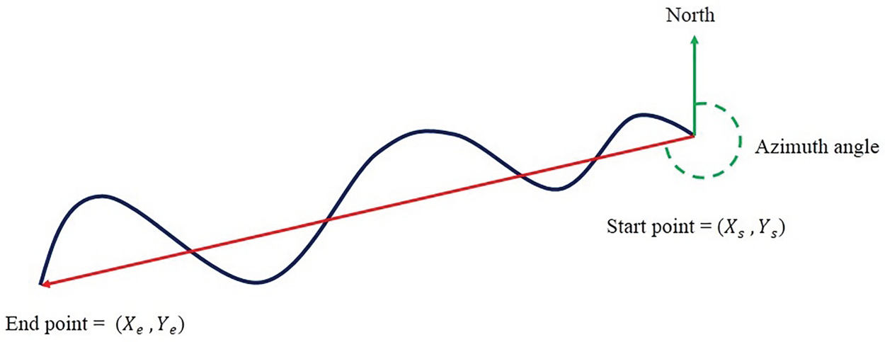
If the target and the most similar extracted points move in the same direction, the PSSP model performs appropriately. However, in our experiments, if these objects move in different directions, the prediction accuracy obtained from the PSSP model will dramatically decrease. Therefore, to improve the accuracy of the PSSP model, a constraint is imposed that declares the absolute difference between the azimuth angle of the target point trajectory and the azimuth angle of the similar point trajectory, which must be less than 22·5°. To recognise which direction the vessel is moving, the start and end points are connected, then the azimuth angle of this connected line is measured by Equations (7) and (8) as illustrated in Figure 3. In Figure 3, the blue line demonstrates a particular trajectory that we incline to measure its azimuth angle, and the red line shows the line that connects the start and end points of the trajectory.
The azimuth angle of a trajectory.

 $$\begin{align} g_{\text{Start}\hbox{-}\text{End}} &= \tan ^{-1}\left| {\frac{X_e - X_s }{Y_e - Y_s}} \right| \end{align}$$
 $$\begin{align} \text{Azimuth}_{\text{Start}\hbox{-}\text{End}} &=\left\{ {{\begin{array}{@{}ll} {g_{\text{Start}\hbox{-}\text{End}} } & {\text{if } \Delta X>0\;\text{and}\;\Delta Y>0} \\ {180-g_{\text{Start}\hbox{-}\text{End}} } & {\text{if } \Delta X>0\;\text{and}\;\Delta Y< 0} \\ {360-g_{\text{Start}\hbox{-}\text{End}} } & {\text{if } \Delta X< 0\;\text{and}\;\Delta Y>0} \\ {180+g_{\text{Start}\hbox{-}\text{End}} } & {\text{if } \Delta X< 0\;\text{and}\;\Delta Y< 0} \end{array} }} \right. \end{align}$$
where  $g_{\text{Start}\hbox{-}\text{End}} $ denotes the bearing angle that is calculated from the coordinates of the start and end points of the trajectory. Consequently, the azimuth angle is measured using the bearing angle (Equation (8)). The 16-point compass rose is used to compare the directions of trajectories based on their azimuth angle. Because the measured angle of each section is 22·5°, the absolute difference of the trajectories is considered less than 22.5°.
3.3. Trajectory-based similarity search prediction (TSSP)
In the TSSP model, the AIS records corresponding to each voyage are considered as a trajectory, and similarity is measured between trajectories instead of individual points. To predict the future locations of the target vessel, the most similar trajectory to the trajectory of the target vessel is extracted from the historical data set. The future locations of the target vessel will be predicted by the extracted trajectory as follows.
3.3.1. Similarity measure phase
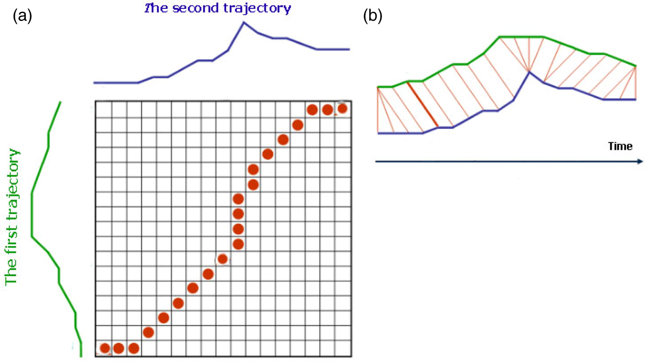
Various similarity measure methods have been introduced or developed based on either time series such as Euclidean distance, edit distance, longest common subsequence, and dynamic time warping (DTW) or geometric shape matching techniques such as Frechet distance and Hausdorff distance (Sharif et al., Reference Sharif, Alesheikh and Tashayo2019]{bib28a}). DTW can be applied to trajectories that have unequal lengths, and is applicable for matching trajectories if information is lacking, for managing local time-shifting, or for addressing parametric data. DTW wraps the first trajectory temporally to minimise the distance to the second trajectory. Elements of the first trajectory then become aligned to the elements of the second trajectory in an optimal way (Sharif and Alesheikh, Reference Sharif and Alesheikh2017), as shown in Figure 4. DTW performs based on elastic shifting of the time axis; therefore, time is not a major component to be investigated.
DTW mechanism: (a) elastic achieved by DTW; (b) trajectory alignments.

DTW is applied to measure how similar two trajectories of distinct voyages are in terms of spatial distance, SOG, and COG. These three DTW distances are in a range from 1 to 2 because of the variety of their units of measurement. The overall weight of ranged values achieved from three DTW results is then calculated by Equation (4) to recognise the trajectory most similar to the target trajectory based on the three criteria.
3.3.2. Location prediction phase
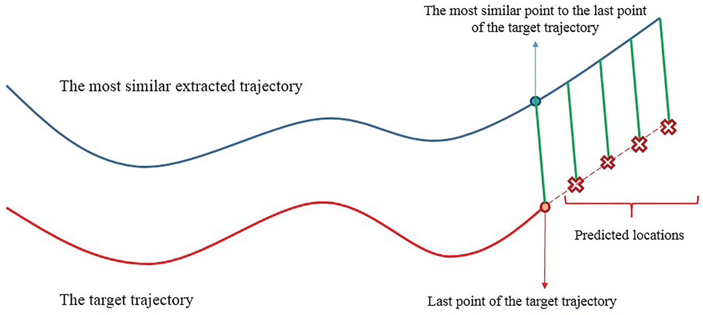
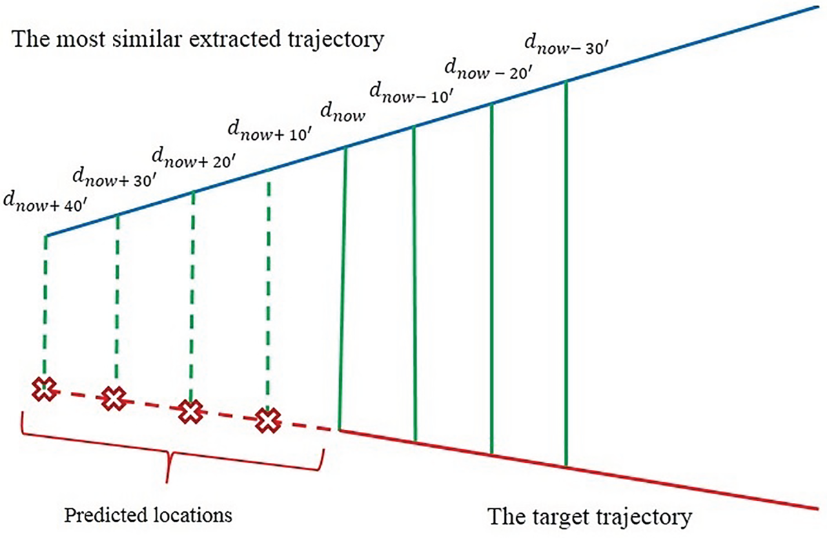
To predict the next location of the target vessel, the spatial distances between the last point of the target trajectory and the point of the detected trajectory, which is the most similar to the last point of the target vessel's trajectory, are calculated using Equation (5). The next location of the target vessel will be predicted using Equation (6) based on the assumption that calculated spatial distances remain constant within the duration of the prediction.
The TSSP model is illustrated in Figure 5. The red line shows the target trajectory, and the blue line indicates the most similar trajectory extracted from the historical trajectories. The green lines represent the spatial distances that are considered constant throughout the prediction. The red crosses show the predicted locations.
Location prediction proposed in the TSSP model.

3.4. Trajectory-based similarity search prediction using LSTM (TSSPL)
Both PSSP and TSSP models assume that the distance between the target trajectory and the trajectory most similar to it remains constant over the prediction duration. However, vessel movement is affected by external contexts, such as wind, waves and sea currents (Kawan et al., Reference Kawan, Wang, Li and Chhantyal2017; Sharif and Alesheikh, Reference Sharif and Alesheikh2018; Kaffash-Charandabi et al., Reference Kaffash-Charandabi, Alesheikh and Sharif2019). In addition, the maritime navigation environment is a complex system that varies over time (Tang et al., Reference Tang, Yin and Shen2019). Consequently, it is highly likely that the spatial distances that have been considered constant in both previous models will change, especially when two trajectories are either converging or diverging. To tackle this issue, an LSTM model is built upon the historical AIS data that can predict spatial distances over the duration of the prediction. Tang et al. (Reference Tang, Yin and Shen2019) developed a LSTM model to predict the future location of vessels. In the proposed model, the first 10 min of a vessel's state, including its location, speed, and course, were observed and inserted into the model as the input sequence, and the location of the vessel at the 20th min was predicted as the output of the LSTM model. However, the similarity search was not used in the LSTM model.
In the TSSPL model, in contrast to the TSSP model, the distance between the target trajectory and the trajectory most similar to it is no longer constant. Therefore, the DTW method is used to find the most similar trajectory. After identifying the trajectory most similar to the target trajectory, spatial distance is calculated between the point on the most similar trajectory that has similarity with the last point of the target trajectory (Equations (5)). In addition, distances are calculated by Equation (5) between the three points before the last point on the target trajectory and their corresponding points on the most similar trajectory. These distances are inserted into the LSTM model as input. The spatial distances predicted by the LSTM model are used to predict the next location at each time interval using Equation (6). An overview of the TSSPL model is illustrated in Figures 6 and 7, for diverging and converging trajectories, respectively. The solid green lines show the calculated distances, the broken green lines show distances predicted using the LSTM model, and the red crosses represent the predicted locations.
The TSSPL model, when two trajectories are diverging.

The TSSPL model, when two trajectories are converging.

3.4.1. Training and implementation of LSTM
LSTMs are special types of recurrent neural networks (RNNs). The basic formula of RNN is shown in Equation (9), where h t stands for the new state, x t indicates the new input, and f shows an activation function with parameters W. RNNs take the previous state represented by h t−1 into account. This characteristic makes them efficient, especially when it comes to modelling sequence problems (Karatzoglou et al., Reference Karatzoglou, Jablonski and Beigl2018). This methodology applies to the present work because distance value at the future timestamp depends on their values at the previous timestamp. However, RNNs suffer from a drawback called vanishing gradients in the backpropagation process (Hochreiter et al., Reference Hochreiter, Bengio, Frasconi, Schmidhuber, Kolen and Kremer2001). In this context, LSRMs were introduced by Hochreiter and Schmidhuber (Reference Hochreiter and Schmidhuber1997), and further improved by Gers et al. (Reference Gers, Schmidhuber and Cummins1999). This was achieved by providing a memory storing and managing mechanism called gated cell. With the aid of this mechanism, LSTMs can store inputs and previous states for a long duration (Karatzoglou et al., Reference Karatzoglou, Jablonski and Beigl2018). A standard notation of LSTMs is defined by Equations (10) and (11).
 $$\begin{align} {h_{t}} &= {f_W} ({{h_{t - 1}}. {x_t}} ) \end{align}$$
 $$\begin{align} {h_t} &= {f_{\text{act}}}({{c_t}} ) \cdot {o_t} \end{align}$$
 $$\begin{align} {c_t} &= {f_t} \cdot {c_{t - 1}} + {i_t} \cdot {f_{\text{act}}} ({{W_x} \cdot {x_t} + {W_h} \cdot {h_{t - 1}} + b} ) \end{align}$$
Equation (10) indicates how the current state can be affected by the output gate represented by o t. f t, i t, f act, W x, and W h stand for the forget gate, gate value, activation function, input hidden, and hidden-hidden layer weight matrices, respectively.
To train the network, historical pre-processed data is used. The most similar trajectory to each trajectory from the database is extracted within the database, then spatial distances are calculated between each pair of trajectories that are similar to each other. These calculated distances are labelled to train the network and adjust the weight matrix by comparing the error between the predicted value and expected value (Figure 8).
Preparing data to feed into the LSTM model.

The structure of the LSTM model is illustrated in Figure 9.  $h_{0} , \; h_{1} , \; h_{2} , \; h_{3} , \; h_{4} $ and
 $x_{0} , \; x_{1} , \; x_{2} , \; x_{3} , \; x_{4} $ represent the hidden state and input, respectively. Finally, the last hidden state passes the sigmoid function to achieve the output. The output derived from a layer of the LSTM model may take a larger value. When this output is inserted into further layers, it can be transformed into even greater values that make the model computationally uncontrollable. This problem is solved with the aid of the sigmoid function by squashing a real value into a fixed interval (between 0 and 1). The input of our LSTM model is defined using a matrix with dimension of 4 × 2 using Equation (12).
Overview of built LSTM model.

 $$\text{Input}= \left[ {\begin{matrix} {{d_1}}\\ {{d_2}}\\ {{d_3}}\\ {{d_4}} \end{matrix}} \right] = \left[ \begin{matrix} (\text{Lon}{\text{g}_{S.1}} - \text{Lon}{\text{g}_{T.1}}) \cdot \text{(La}{\text{t}_{S.1}} - \text{La}{\text{t}_{T.1}})\\ (\text{Lon}{\text{g}_{S.2}} - \text{Lon}{\text{g}_{T.2}}) \cdot (\text{La}{\text{t}_{S.2}} - {\text{Lat}_{T.2}})\\ (\text{Lon}{\text{g}_{S.3}} - \text{Lon}{\text{g}_{T.3}}) \cdot (\text{La}{\text{t}_{S.3}} - \text{La}{\text{t}_{T.3}})\\ (\text{Lon}{\text{g}_{S.4}} - \text{Lon}{\text{g}_{T.4}}) \cdot (\text{La}{\text{t}_{S.4}} - \text{La}{\text{t}_{T.4}}) \end{matrix}\right]$$
3.4.2. Evaluation of LSTM
To train the LSTM model, historical trajectories are divided into two sets: a primary training set and a test set, in a ratio of eight to two. The initial training set is then divided into two sets: a training set and a validation set, in a ratio of seven to three. The model is trained using the data in the training set. The validation set is used during the training process to validate the model for enhancing its generalisation ability. The test data are used to achieve the prediction result and assess the performance of the model.
To evaluate the performances of the LSTM model, mean squared error (MSE) and r-squared are used as the evaluation metrics (Equations (13) and (14)).
 $$\begin{align} \textrm{MSE} = \frac{1}{n}\sum_{i = 0}^n {({{y_i} - \widehat{{y_i}}})^2} \end{align}$$
 $$\begin{align} {R^2} = 1 - \frac{{\sum_{i = 0}^n {{({{y_i} - \widehat {{y_i}}})}^2}}}{{\sum_{i = 0}^n {{({{y_i} - \overline {{y_i}} })}^2}}} \end{align}$$
where y i,  $\widehat{{y_{i}}}$, and
 $\overline{{y_{i}}}$ represent the actual value, predicted value, and the average of all real values, respectively. MSE indicates how close the actual values are to the model's predicted values. MSE is an absolute measure of fit, whereas R 2 is a relative measure of fit.
4. EXPERIMENTAL STUDY
The Strait of Juan de Fuca or Georgia on the west coast of the USA, which is located at latitude 48N to 48·6N and longitude −125·9 W to −125·2 W, is selected as the area of interest (Figure 10). The entrance of the Strait of Juan de Fuca is a congested maritime environment with hundreds of ships passing.
The Strait of Juan de Fuca, west coast of USA.

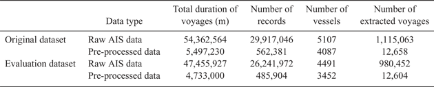
Two different datasets provided by Marinecadastre (2019) are used in this study: one from March 2017 for creating the database and the other from February 2017 for the evaluation of the proposed models. In Table 1, the information extracted from raw AIS data and that extracted from pre-processed data are compared. The considerable difference between these two datasets is that only mobile vessels are preserved.
Comparison between raw data and pre-processed data related to original and evaluation datasets.

5. RESULTS AND DISCUSSION
To evaluate the applicability of the PSSP, TSSP, and TSSPL models, the future positions of the 89 distinct vessels at time intervals of 10, 20, 30, and 40 min have been predicted. To assess the models' accuracies, the Haversine distance between the actual position and the predicted position is calculated by Equation (1). The calculated distance is defined as the error of prediction that indicates the distance on the Earth's surface between real and predicted positions. According to the importance of the spatial dimension (w d), the weight is set at 0·6. The weights of the speed (w s) and course (w c) criteria are set at 0·2.
Table 2 provides the average prediction error of the 89 target
Location prediction errors (in kilometres).

vessels at different prediction durations. As can be seen, in the TSSPL model prediction error decreases by 53·6%, 54·2%, 55·8%, and 55·2% at the time intervals of 10, 20, 30, and 40 min, respectively. Compared with the PSSP model, the TSSPL model shows its efficiency, especially in long-term prediction. As can be inferred from Table 2, the prediction errors for all three models increase during the prediction time. In the PSSP and TSSP models, this occurs because, as time passes, the spatial distances remain constant. For the TSSPL model, the reason can be attributed to the fact that spatial distances are predicted with the help of previous spatial distances predicted by the LSTM model. Therefore, the error of predicted spatial distance in each timestamp would affect the error of predicted spatial distance in the next timestamps.
A general comparison between the accuracy of the models is demonstrated in Figure 11. The vertical and horizontal axes show the values of the prediction error and the time intervals of the prediction, respectively. The slope of the TSSPL model, which indicates error changes over time, is less than that of the other two models. This assures more reliable prediction, especially in the longer term; the slopes reveal an increase in the prediction error as the duration of prediction continues.
Comparison of performances of trajectory prediction models over time.

Compared with similar researches, the proposed models perform better in terms of prediction accuracy. The PSSP model achieved accuracy of 0·842, 1·7, 2·582, and 3·501 kilometres for the prediction times of 10, 20, 30, and 40 min, respectively. In addition, prediction error has decreased significantly by 40·85% for the TSSP model compared with the PSSP model and by 23% for the TSSPL model compared with the TSSP model. The results obtained justify the applicability of the proposed models for the long-term prediction that is highly required for vessel traffic monitoring and collision avoidance. However, relying solely on the quantitative results reported is not reliable because each research study conducts its evaluations on different regions and does not consider the spatial variability within and between regions (Graser et al., Reference Graser, Schmidt, Dragaschnig and Widhalm2019).
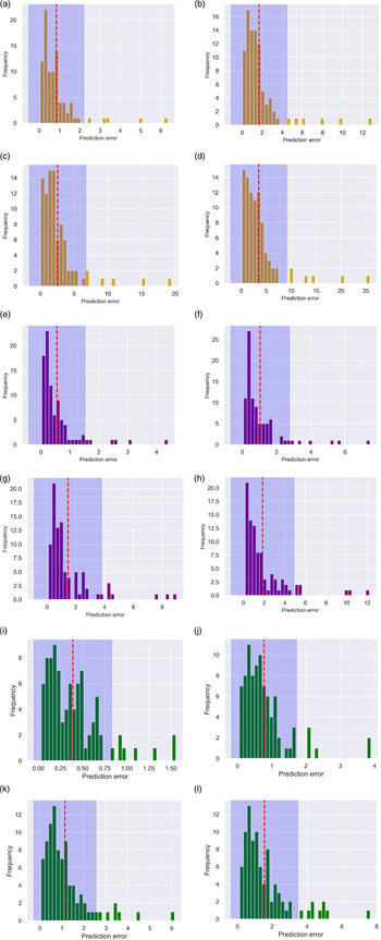
Error distribution analysis has been conducted to assess the models' performance quantitatively. Figure 12 shows the frequency histograms of the error predictions for the next 10, 20, 30, and 40 min. The vertical and horizontal axes indicate the number of predictions for each error and the value of prediction error, respectively. The red line refers to the mean value (μ ) of the histogram, and the blue area demonstrates the interval  $\mu -\sqrt{2}\sigma $ and
 $ \mu +\sqrt{2} \sigma $, where σ stands for the standard deviation. Concerning the Chebyshev's inequality (Alsmeyer, Reference Alsmeyer and Lovric2011), at least 50% of values are located within the blue area. The mean values of the TSSPL model are lower than the PSSP and TSSP models for all prediction times.
Frequency histograms of error prediction: (a)–(d) for the PSSP model, (e)–(h) for the TSSP model, and (i)–(l) for the TSSPL model for next 10, 20, 30, and 40 min, respectively.

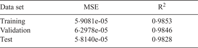
The constructed LSTM model has been evaluated using metrics described in Section {3.4.2}. Table 3 provides quantitative results of the model's performance on the training, validation, and test data sets. As can be seen in Table 3, MSEs related to the training and validation data sets are very close to each other, which means the LSTM model has been trained. In addition, MSE corresponding to the test data set is very close to zero, indicating that the model is perfectly able to predict new data. The values of the two indices during the 1,000 epochs are shown in Figure 13.
Quantitative result of the model's performance: (a) r-squared values on training dataset; (b) r-squared values on validation data set; (c) MSE values on training data set; (d) MSE on validation data set.

Evaluation of the model performance.

In the PSSP model, three different constraints moving in the same direction were set up on the target trajectory and the most similar extracted trajectory. The performance of the PSSP model was evaluated by applying each constraint based on prediction error and the best constraint was chosen as follows.
• Azimuth constraint: This constraint declares that the absolute difference between the azimuth angle of the target point trajectory and the azimuth angle of the similar point trajectory is less than 22·5°.
• COG constraint: As COG determines the actual direction of the vessel, this constraint states that the mean values of COG for the target vessel and the most similar extracted vessel must be the same. In other words, both values must be either negative or positive numbers. If the COG value of two trajectories is positive, it means that they are moving towards the east. Likewise, when the COG values of two trajectories are negative, it means that they are moving towards the west.
• Longitude constraint: Another way to distinguish the vessel direction is to calculate the difference between the longitudes of the first and last points of the trajectory, which is called a longitude difference. This constraint expresses that the sign of longitude difference must be the same for the target trajectory and the most similar extracted trajectory.
Evaluation of the performance of each imposed constraint is provided in Table 4. As can be inferred, the azimuth constraint shows the best performance in terms of prediction error compared with the other constraints.
Evaluation of the PSSP model performance with different constraint (in kilometres).

To assess the robustness of each defined constraint, 353 distinct trajectories are inserted into the PSSP model as input trajectories. The number of trajectories that the model can predict is then counted. Robustness value is calculated by Equation (15).
 $$\text{Robustness value} = \frac{{\textrm{Predicted trajectories}}}{{\textrm{Input trajectories}}}\times 100$$
Robustness values for azimuth, COG, and longitude constraints are 66%, 56%, and 55%, respectively. Figure 14 compares the applicability of each constraint. The orange and blue bars, respectively, refer to the input trajectories and the number of trajectories that the PSSP model can predict.
Robustness test of different constraints.

6. CONCLUSION
This research contributes to the prediction of vessels' movements for short and long time durations. Three distinct similarity-based models, namely PSSP, TSSP, and TSSPL, are proposed. In the PSSP model, trajectories are considered as individual points and the most similar point to the target point is found. The prediction is performed by using the most similar point found from the database. However, two sampling points from two distinct trajectories are remarkably the same, whereas the moving objects' behaviours are in different directions. To find out how similar the moving objects' behaviours will be in the future, the similarity between the two trajectories is measured by using the TSSP model. This approach results in a remarkable increase in the accuracy of predictions compared with the PSSP model. The PSSP and TSSP models are based on the assumption that the distance between the target trajectory and the trajectory most similar to it will remain constant. However, because of the dynamic maritime context, this distance is changing within the duration of the prediction. To address this issue, the third proposed model, TSSPL, predicts the mentioned distance using the LSTM model constructed on historical trajectories. Applying the TSSPL model results in a steady decrease in prediction error compared with the TSSP model. The results reveal that the third model is more accurate than the other two models, and it can be utilised to predict a vessel's trajectory effectively, particularly in long-term prediction. This research provides valuable information for coastguards, port management, and insurance companies, supporting them to make their decisions based on knowledge. Moreover, the three proposed models not only show applicability in terms of vessel trajectory prediction but they can also be used in other applications, for example, prediction of hurricanes, and human, and animal trajectories. For further studies, the authors suggest considering the inclusion of contextual information in the similarity measures and location predictions of trajectories. Environmental contexts such as wind, wave, and weather conditions have immense effects on the movement of vessels so that they may deviate from their normal path.