1. Introduction
Providing sufficient income in retirement is one of the principal problems faced by individuals. In response to this need, insurance and financial companies have provided a large variety of useful and innovative products. Among these products are the guaranteed lifetime withdrawal benefit (GLWB) riders attached to variable annuity products. These contracts allow customers to withdraw a fixed percentage of their benefit base, regardless of whether their investment fund has enough money in it to sustain the withdrawal at that time. The customer chooses the date from which the withdrawals will begin. The guaranteed withdrawal percentage goes up with age, and so delaying initiation of the withdrawals will provide a larger annual income.
At the commencement of the contract, the benefit base is equal to the premiums paid. In many current contracts, the benefit base has a “step-up” or “ratchet” feature. In these riders, the benefit base may move upwards on the policy anniversary if the investment returns have caused the fund to increase. Most contracts allow for step-ups only before benefits commence, but contracts exist that allow step-ups even after the benefits have commenced. A good description of the contracts and market can be found in Drinkwater et al. (Reference Drinkwater, Iqbal and Montminy2013). They find typical fees of 233 basis points (BP), most frequently charged as a percentage of the benefit base.
These contracts provide policyholders with several advantages relative to traditional annuity products. The most important is added liquidity. Standard annuity contracts do not allow policyholders to withdraw funds from the reserve since this would result in serious anti-selection issues as unhealthy policyholders withdraw rather than continue periodic payments. GLWB riders, however, allow partial or full withdrawal of the remaining funds if the fund balance remains above zero. When this option is exercised, the benefit base and the associated guaranteed withdrawals are adjusted proportionately. If the policyholder dies with a positive fund balance, the account is paid to a beneficiary as a death benefit. This additional feature provides policyholders with liquidity in the case of adverse health shocks and additional medical expenses. It also allows the policyholder to provide a death benefit to dependents.
In the United States, the tax-deferred status of the investment income in the funds supporting these riders is a major complication. For example, see Moenig and Bauer (Reference Moenig and Bauer2015), for the impact of taxes on the closely related GMWB riders. Investors in the United States can fund the GLWB variable annuity with pre-tax funds and will defer taxes on the investment income until it is realized through withdrawals. Withdrawals are taxed as ordinary income. This includes all withdrawals, both those that are supported by the fund and those that are made after the fund value has dropped to zero.
In New Zealand (NZ), however, the thought behind retirement tax policy is noticeably different. There is, in general, no tax deferral of either retirement contributions or investment income. A GLWB would be funded with post-tax funds. The investment income would be taxed when earned and decrease the fund as a result. The withdrawals, however, would be tax-free until they exceeded the benefit base (or were no longer supported by the fund) at which point the withdrawals would become taxable as income. A good discussion of the rationale behind the differing tax treatment in NZ and the effect on annuity products can be found in several papers by St. John (Reference Bauer, Gao, Moenig, Ulm and Zhu2003, Reference St. John2007a, Reference St. John2007b, Reference St. John2009).
This difference in tax treatment has a significant effect on the risk-return profile of the funds underlying the GLWB. This effects both the desirability of the contract to retirees and the fees charged on a risk-neutral basis by the issuer.
2. The Model of GLWBs in Different Tax Regimes
We model a representative variable annuity product in the NZ marketplace. An individual who chooses to begin his withdrawals at age 65 will receive a guaranteed right to 5% withdrawal of the strike value per year for life, regardless of the fund performance. If the individual chooses to wait until age 66, the guaranteed withdrawal rate will rise to 5.1% and will increase at 0.1% per year until reaching 7.5% at age 90. The strike value is set to the initial fund amount at the initiation of the contract and has a ratchet feature so that the strike at later ages is set to the maximum fund amount on a policy anniversary.
The fund is required to be invested conservatively, which we model as a base scenario volatility of 14%. If the fund has a positive balance, fees and withdrawals are deducted from the fund fortnightly. If the fund has a zero balance, guaranteed withdrawals are paid directly by the company. An individual can withdraw a positive fund balance at any time with a proportional reduction in the strike value. We model this conservatively as a death benefit with no extra (non-guaranteed) withdrawals prior to death. In agreement with Huang et al. (Reference Huang, Milevsky and Salisbury2014), we typically find no benefit in delaying the initiation of withdrawals under any tax regime.
Under the US tax treatment, the variable annuity with a GLWB will be purchased with pretax funds. The internal build-up of the funds will not be taxed until withdrawn. The guaranteed withdrawals are taxed as income, starting from the first dollar withdrawn, and the fund paid out as a death benefit is also fully subjected to taxes.
Under the NZ tax treatment, the variable annuity with a GLWB will be purchased with post-tax funds. The internal investment returns, both gains and losses, are taxed as income when they occur. The fund paid out as a death benefit is not taxed. The guaranteed withdrawals are also not taxed until the fund drops to zero, at which point the withdrawals are taxed as income.
The value of the GLWB is determined using risk-neutral option pricing methods. This approach assumes that the value is being calculated from the perspective of a seller who is able to diversify the mortality risk and hedge the remaining market risk in a complete market. A description of this approach can be found in Bauer et al. (Reference Bauer, Gao, Moenig, Ulm and Zhu2008). This approach has been used extensively in the valuation of options in variable annuities. A good overview can be found in the references in Table 1 in Bauer et al. (Reference Bauer, Gao, Moenig, Ulm and Zhu2017).
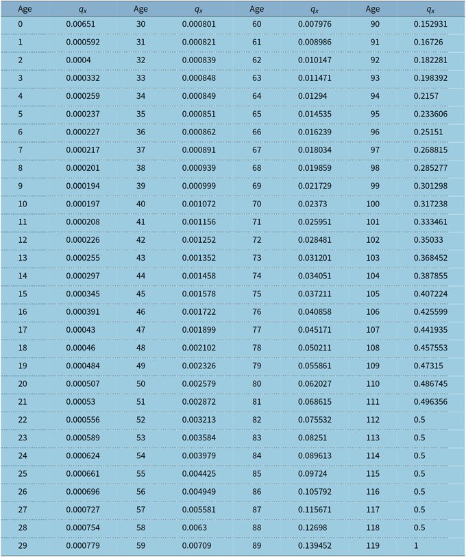
1994 group annuity mortality (GAM) male table

We use a trinomial lattice with 2-week time steps. The lattice has two stages. In the first stage, the probabilities of an up, middle and down move are calibrated so that the fund grows at the risk-free rate and has the appropriate volatility. The second stage removes taxes, withdrawals and fees from the fund. Once the fund drops to zero, the value is treated as annuity. The values are discounted through the lattice at the risk-free rate. In both regimes, the fees are a percentage of the strike (not the fund) and are set so that the risk-neutral value of the option to the company is zero, assuming that the company can create a hedge in a complete market.
The base scenario is a risk-free rate of 3%, a volatility of 14% (i.e. conservative investments) and a tax rate of 28% (the NZ tax rate on portfolio investment entities). These rates will be assumed in the analysis, unless different parameter values are stated explicitly. We performed sensitivity analysis as well, allowing the risk-free rate to vary between 0.0% and 5.0% in steps of 0.5%, the volatility to vary between 0% and 30% in steps of 1% and the tax rate to vary between 0% and 28% in steps of 2%. Mortality follows the 1994 GAM male table with values shown in Table 1. We choose a starting account value and starting strike value of $1,000 in the analysis that follows.
3. Analysis of Results
The most obvious difference between the two tax regimes is that contracts in the NZ tax regime are always less valuable to the policyholder than contracts in the US tax regime. This is due to taxes being collected earlier in NZ and therefore being discounted less heavily. Since the total value is $1,000 and the company value is set to $0, the policyholder value must be smaller in the NZ regime if the present value of taxes is larger.
The value to US policyholders is straightforward to compute. It can be shown that the US tax regime is equivalent to one where the government owns a share of the contract equal to the tax rate τ and the policyholder owns an untaxed share of the contract equal to 1 − τ. The value to the US policyholder is, therefore, $1000(1 − τ). The value to a NZ policyholder is always less than $1000(1 − τ).
3.1 Comparison of risk-neutral GLWB prices
We begin by examining the BP charges required to break even in the two tax regimes. This matters from the perspective of the issuer since a lower fee requirement would make the product sell more easily. Because the policyholder effectively owns an untaxed share of the contract, the US BP charges can be computed by ignoring taxes entirely. Charges are, therefore, independent of taxes and equal to 84.48 basis points in the base scenario.
There are two competing forces at work in the NZ tax regime. First, the earnings of the fund are reduced by the tax rate. This makes the option more likely to go into the money and increases the charges relative to the corresponding US case. Second, the volatility of the fund is reduced since high returns are taxed away and low returns receive a tax credit against income. This decreases the option value and decreases the charges relative to the corresponding US case. The first effect dominates at high values of the risk-free rate and low values of volatility. The second effect dominates when the risk-free rates are low or the volatility is high.
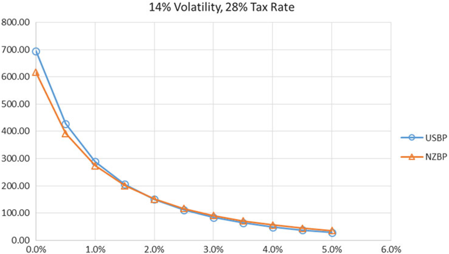
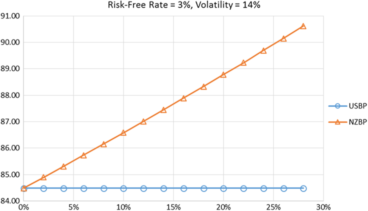
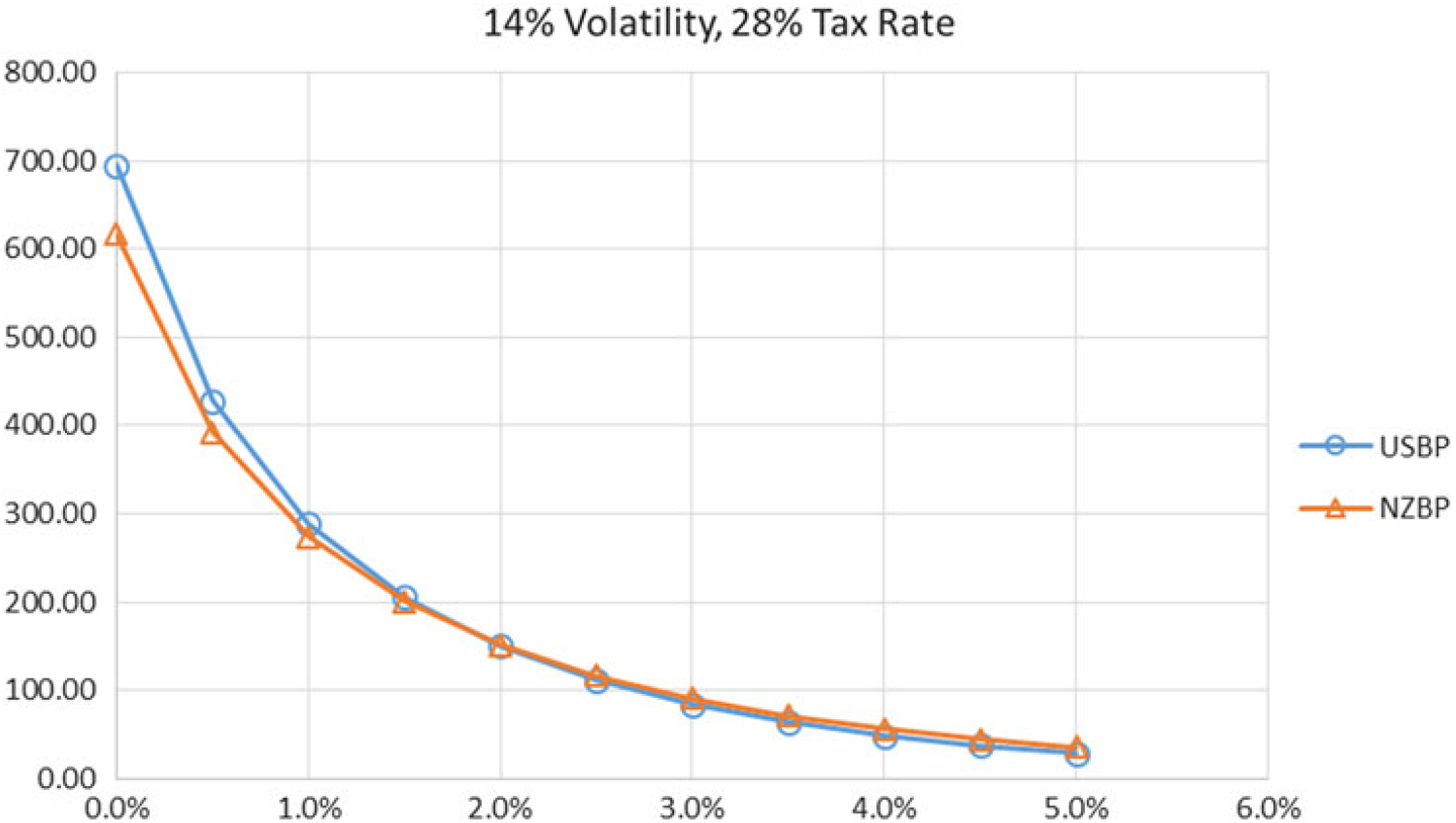
The interplay of these effects can be seen in Figures 1 and 2. Figure 1 plots the BP charges against the risk-free rate for the US and NZ tax regimes. The charges in the NZ tax regime are seen to be lower than the US charges when the risk-free rate is low and are higher than the US charges when the risk-free rate is high. Both sets of charges decrease as the risk-free rate increases as the option is less likely to be in the money when its expected return is larger.
BP charges versus risk-free rates in the US and NZ tax regimes.
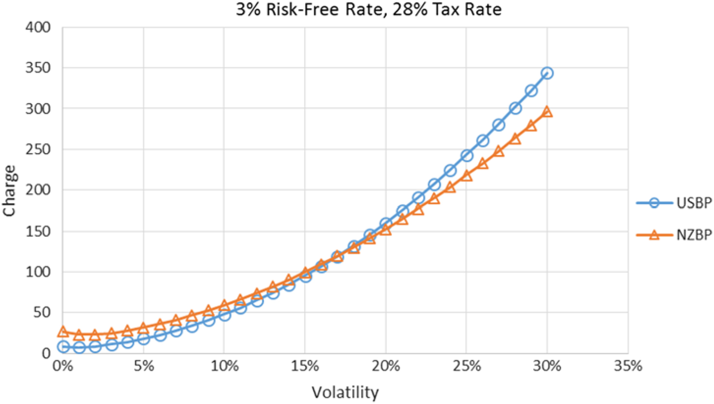
BP charges versus volatility in the US and NZ tax regimes.

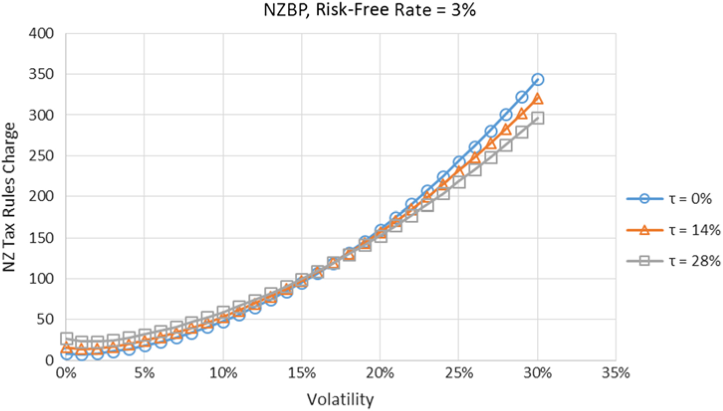
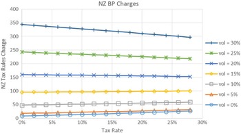
Figure 2 plots the BP charges against the volatility for both regimes. The charges in the NZ tax regime are seen to be higher than the US charges when the volatility is low and are lower than the US charges when the volatility is high. Both sets of charges decrease as the risk-free rate increases as the option is less likely to be in the money when its expected return is larger. The two curves cross at a volatility of about 17%. Interestingly, this crossing point appears to be independent of the tax rate, as can be seen in Figure 3, where all the NZ curves cross at 17% when the risk-free rate is 3%.
BP charges versus volatility in the NZ tax regime for various tax rates.
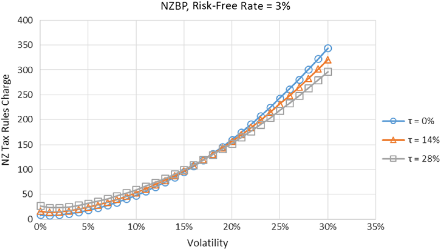
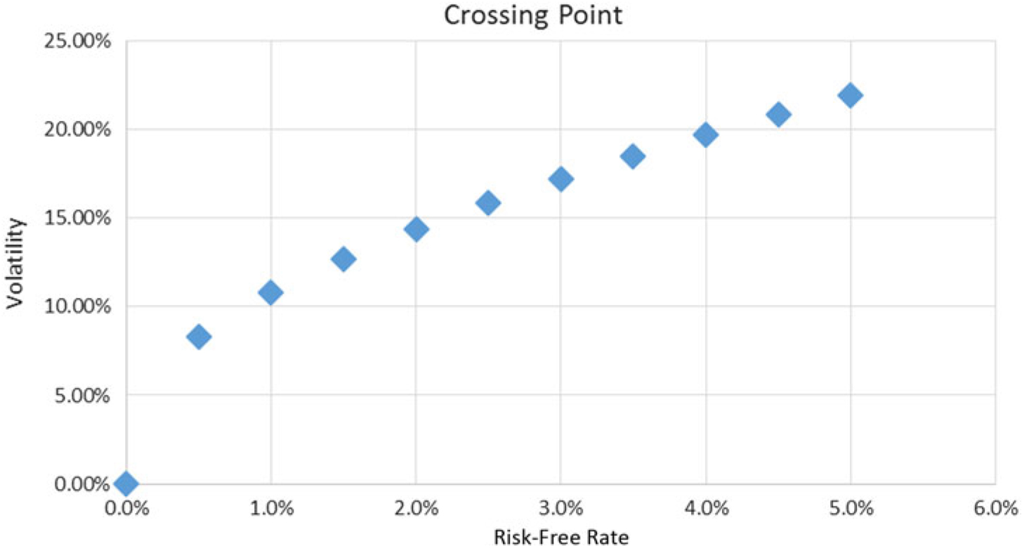
The independence of crossing point and tax rate remains roughly true for all values of the risk-free rate between 0% and 5%. Figure 4 shows the crossing point volatility where the US and NZ charges are equal as a function of risk-free rate.
Crossing points where NZ and US GLWB charges are roughly equal.

The NZ basis point charges are equal to those in the US tax regime when taxes are zero and are roughly linear in the tax rate. This can be seen in Figure 5 which plots both the NZ and US charges against the tax rate in the base scenario. It turns out that the fees charged are quite stable with tax rate for a given volatility level, as shown in Figure 6.
BP charges versus tax rate.

NZ BP charges versus tax rate for various volatilities.

3.2 Comparison of risk-neutral GLWB policyholder values
We now look at the policies from the perspective of the policyholder. The value of the GLWB is always lower in NZ than in the US tax regime due to the earlier collection of taxes. In one sense, this implies that a NZ GLWB is less attractive than the US GLWB. However, this is not the most relevant comparison since the option of purchasing a US GLWB is not available to a NZ tax resident. The nearest substitute available to a NZ tax resident is a conventional payout annuity so that is the comparison that will be made in the following analysis.
We calculate the expected present value of the annuity in both tax regimes. In the United States, we make the same assumptions for the annuity as we did for the GLWB. The annuity is bought with pre-tax funds, investment earnings are not taxed and payouts are taxed when received. The payout rate is set to the actuarially fair value. This results in a value of $1000(1 − τ) to the policyholder, for the same reason as in the GLWB case. If the products are priced at zero profit, the value of the GLWB and the annuity will be the same in the US tax regime.
In NZ, we assume that the investment income is taxed, but the annuity is received tax-free. There are complications that arise from the differences in individual and corporate investment tax rates. Details can be found in St. John (Reference St. John2009). We are not modelling those issues in order to isolate the effect of tax regime by itself. Again, we set the payout rate to the actuarially fair value, including the effect of taxes.
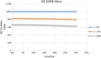
We find that annuities are typically worth more than the GLWB contracts to policyholders in the NZ regime. In other words, the government takes a larger share of the expected present value of the initial investment in GLWB contracts relative to annuity contracts. This occurs because the government treats GLWB contracts as individual accounts and taxes both investment income and payments that exceed the initial investment plus returns. On the other hand, the government does not tax annuity payments that exceed the initial investment, treating the fund as a pooled investment. The loss to the policyholder increases with the volatility of the fund, as shown in Figure 7. The value to the policyholder is surprisingly stable with respect to changes in the volatility of the fund, as shown in Figure 8.
Policy values versus volatility.

NZ GLWB values versus volatility for different tax rates.

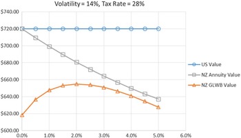
US annuity and GLWB values are independent of the risk-free rate. Payouts are larger in high interest rate environments but are discounted more to compensate. NZ annuity values fall with interest rates, since taxation occurs earlier and the effect of this is more pronounced at higher rates. NZ GLWB values rise and then fall with rates. This is due to the interplay between growth rates, discount rates and fees charged, since the payout rate is independent of the interest rate for a GLWB. These features are shown in Figure 9.
Policy values versus risk-free rate.

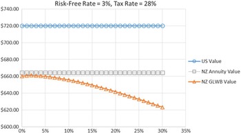
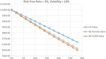
The annuity and GLWB values fall roughly linearly with the tax rate. For the US annuity values, the decline is exactly linear. The NZ values decline slightly more rapidly at low tax rates and less rapidly at high ones. The relationship between values and tax rate are shown in Figure 10.
Policy values versus tax rate.

4. Conclusions
The differing tax treatment of GLWB in countries with tax-deferred and non-tax-deferred retirement schemes has a significant effect on the value of these products in these markets. If risk-neutral pricing is used and consumers behave as though they are in a complete market, a GLWB and a payout annuity will be equally valuable to a policyholder in a tax-deferred environment.
However, the GLWB will be less valuable than a payout annuity in this risk-neutral setting if the tax regime does not allow for deferral of taxes. The fees charged for the product will be lower with tax deferral when expected returns are high and will be higher with tax deferral when expected returns are low. While this analysis suggests that GLWB products are not valuable in non-tax-deferred environments, it assumes a complete market environment for the policyholder. It remains possible that an analysis in a utility framework that takes liquidity into account may change this conclusion.