2.1 Introduction of the virtual velocity

In a three-dimensional fluid flow, the Eulerian velocity $\boldsymbol{u}=(u_{x},u_{y},u_{z})$ is governed by the NS equations, including the continuum equation

(2.1) $$\begin{eqnarray}\frac{\unicode[STIX]{x2202}\unicode[STIX]{x1D70C}}{\unicode[STIX]{x2202}t}+\unicode[STIX]{x1D735}\boldsymbol{\cdot }(\unicode[STIX]{x1D70C}\boldsymbol{u})=0,\end{eqnarray}$$

the momentum equation

(2.2) $$\begin{eqnarray}\frac{\unicode[STIX]{x2202}\boldsymbol{u}}{\unicode[STIX]{x2202}t}+(\boldsymbol{u}\boldsymbol{\cdot }\unicode[STIX]{x1D735})\boldsymbol{u}=\unicode[STIX]{x1D735}\unicode[STIX]{x1D6F1}+\boldsymbol{F},\end{eqnarray}$$

the energy equation and the equation of state. Here, $\unicode[STIX]{x1D6F1}=-p/\unicode[STIX]{x1D70C}+\unicode[STIX]{x1D6EF}$ denotes a generalized potential with the pressure  $p$ , the density $\unicode[STIX]{x1D70C}$ and the potential $\unicode[STIX]{x1D6EF}$ of conservative body forces, and

(2.3) $$\begin{eqnarray}\boldsymbol{F}=\frac{1}{\unicode[STIX]{x1D70C}}(\unicode[STIX]{x1D735}\boldsymbol{\cdot }\unicode[STIX]{x1D749})+p\unicode[STIX]{x1D735}\left(\frac{1}{\unicode[STIX]{x1D70C}}\right)+\boldsymbol{f}\end{eqnarray}$$

denotes a generalized non-ideal force term, where $\unicode[STIX]{x1D749}$ is the viscous stress tensor and $\boldsymbol{f}$ is the non-conservative external body force per unit mass.

In a non-ideal flow, the three terms on the right-hand side of (2.3) respectively denote the viscous term in most real flows, the baroclinic term, e.g. in compressible flows and combustion, and the non-conservative body force term, e.g. the Lorentz force in MHD flows.

Taking curl of (2.2) yields the transport equation

(2.4) $$\begin{eqnarray}\frac{\unicode[STIX]{x2202}\unicode[STIX]{x1D74E}}{\unicode[STIX]{x2202}t}-\unicode[STIX]{x1D735}\times (\boldsymbol{u}\times \unicode[STIX]{x1D74E})=\unicode[STIX]{x1D735}\times \boldsymbol{F}\end{eqnarray}$$

for the vorticity $\unicode[STIX]{x1D74E}\equiv \unicode[STIX]{x1D735}\times \boldsymbol{u}$ . Helmholtz’s vorticity theorem illustrates a frozen-in nature of  $\unicode[STIX]{x1D74E}$ in ideal flows with $\boldsymbol{F}=0$ , whereas it breaks down in non-ideal flows, or, more precisely, in non-circulation-preserving flows with $\unicode[STIX]{x1D735}\times \boldsymbol{F}\neq 0$ (see Truesdell Reference Truesdell1954). We remark that only a few non-ideal flows with trivial vortex dynamics are circulation-preserving, e.g. steady plane Couette and Poiseuille flows, so we do not strictly distinguish non-ideal and non-circulation-preserving flows in the present study.

Equivalently, Kelvin’s circulation theorem is not valid for non-ideal flows with $\unicode[STIX]{x1D735}\times \boldsymbol{F}\neq 0$ , i.e. the material derivative

(2.5) $$\begin{eqnarray}\frac{\text{D}}{\text{D}t}\equiv \frac{\unicode[STIX]{x2202}}{\unicode[STIX]{x2202}t}+\boldsymbol{u}\boldsymbol{\cdot }\unicode[STIX]{x1D735}\end{eqnarray}$$

of the circulation $\unicode[STIX]{x1D6E4}\equiv \oint _{{\mathcal{C}}}\boldsymbol{u}\boldsymbol{\cdot }\text{d}\boldsymbol{l}$ round any closed material curve ${\mathcal{C}}$ that bounds an open material surface ${\mathcal{S}}$ has

(2.6) $$\begin{eqnarray}\frac{\text{D}\unicode[STIX]{x1D6E4}}{\text{D}t}=\int _{{\mathcal{S}}}(\unicode[STIX]{x1D735}\times \boldsymbol{F})\boldsymbol{\cdot }\boldsymbol{n}\,\text{d}{\mathcal{S}}\neq 0,\end{eqnarray}$$

where $\text{d}\boldsymbol{l}$ denotes a line element and $\boldsymbol{n}$ the normal of  ${\mathcal{S}}$ .

In order to extend Kelvin’s theorem to non-ideal flows, we assume that there exists a smooth virtual velocity $\boldsymbol{v}$ determined by

(2.7) $$\begin{eqnarray}\unicode[STIX]{x1D735}\times (\boldsymbol{v}\times \unicode[STIX]{x1D74E})=\unicode[STIX]{x1D735}\times (\boldsymbol{u}\times \unicode[STIX]{x1D74E}+\boldsymbol{F})\end{eqnarray}$$

so that $\unicode[STIX]{x1D74E}$ is transported in $\boldsymbol{v}$ as

(2.8) $$\begin{eqnarray}\frac{\unicode[STIX]{x2202}\unicode[STIX]{x1D74E}}{\unicode[STIX]{x2202}t}-\unicode[STIX]{x1D735}\times (\boldsymbol{v}\times \unicode[STIX]{x1D74E})=0.\end{eqnarray}$$

This type of the virtual velocity was first introduced by Newcomb (Reference Newcomb1958) for the frozen-in motion of magnetic field lines in conducting flows, and it was revisited in the context of both HD and MHD flows (e.g. Greene Reference Greene1993; Hornig & Schindler Reference Hornig and Schindler1996; Zhu Reference Zhu2017).

2.2 Virtual conservation theorems

Based on the virtual velocity, Kelvin’s theorem for ideal flows can be extended to non-ideal flows. Specifically, the virtual material derivative

(2.9) $$\begin{eqnarray}\frac{\text{D}_{v}}{\text{D}_{v}t}\equiv \frac{\unicode[STIX]{x2202}}{\unicode[STIX]{x2202}t}+\boldsymbol{v}\boldsymbol{\cdot }\unicode[STIX]{x1D735}\end{eqnarray}$$

of $\unicode[STIX]{x1D6E4}$ vanishes, where $\unicode[STIX]{x1D6E4}$ is driven by the virtual velocity. This conservation law will be referred to as virtual Kelvin’s theorem (see its proof in supplementary material available at https://doi.org/10.1017/jfm.2018.1014).

Theorem 1 (virtual Kelvin’s theorem).

Let ${\mathcal{C}}(t)$ be a closed curve moving with a globally smooth virtual velocity  $\boldsymbol{v}$ . Then the circulation $\unicode[STIX]{x1D6E4}$ is a virtual Lagrangian scalar as

(2.10) $$\begin{eqnarray}\frac{\text{D}_{v}\unicode[STIX]{x1D6E4}}{\text{D}_{v}t}=0.\end{eqnarray}$$

Therefore, the flow of the virtual carrier velocity is circulation-preserving, and it is a special class of flows of significant interest (see Truesdell Reference Truesdell1954; Wu, Ma & Zhou Reference Wu, Ma and Zhou2006). Then it is straightforward to extend the classical conservation theorems for vorticity kinematics in ideal flows to non-ideal flows with a smooth, circulation-preserving virtual velocity. The modified theorems below are referred to as virtual Helmholtz’s theorem, virtual Ertel’s theorem and the virtual conservation of helicity (see their proofs in the supplementary material). Similar extensions were discussed in different contexts for HD and MHD flows (see Greene Reference Greene1993; Hornig & Schindler Reference Hornig and Schindler1996; Wu et al. Reference Wu, Ma and Zhou2006). Additionally, more vorticity-based conservation laws (e.g. Cheviakov & Oberlack Reference Cheviakov and Oberlack2014) may be able to be extended to non-ideal flows.

Strictly speaking, the requirement of $\boldsymbol{v}$ for flux-conservation in (1) of virtual Helmholtz’s theorem is stronger than that for line-preserving in (2). In other words, for only satisfying the virtual line-preserving in (2), the constraint (2.7) of $\boldsymbol{v}$ can be relaxed to

(2.15) $$\begin{eqnarray}\unicode[STIX]{x1D735}\times (\boldsymbol{v}\times \unicode[STIX]{x1D74E})=\unicode[STIX]{x1D735}\times (\boldsymbol{u}\times \unicode[STIX]{x1D74E}+\boldsymbol{F})-\unicode[STIX]{x1D706}\unicode[STIX]{x1D74E},\end{eqnarray}$$

with an arbitrary scalar $\unicode[STIX]{x1D706}$ (see Truesdell Reference Truesdell1954).

Theorem 3 (virtual Ertel’s theorem).

Let  $\unicode[STIX]{x1D719}$  be a virtual Lagrangian scalar convected by a globally smooth virtual velocity as

(2.16) $$\begin{eqnarray}\frac{\text{D}_{v}\unicode[STIX]{x1D719}}{\text{D}_{v}t}=0,\end{eqnarray}$$

with

(2.17) $$\begin{eqnarray}\frac{\unicode[STIX]{x1D74E}}{\unicode[STIX]{x1D70C}}\boldsymbol{\cdot }\unicode[STIX]{x1D735}\unicode[STIX]{x1D719}=0\end{eqnarray}$$

at the initial time, and then $(\unicode[STIX]{x1D74E}/\unicode[STIX]{x1D70C})\boldsymbol{\cdot }\unicode[STIX]{x1D735}\unicode[STIX]{x1D719}$ is also a virtual Lagrangian scalar as

(2.18) $$\begin{eqnarray}\frac{\text{D}_{v}}{\text{D}_{v}t}\left(\frac{\unicode[STIX]{x1D74E}}{\unicode[STIX]{x1D70C}}\boldsymbol{\cdot }\unicode[STIX]{x1D735}\unicode[STIX]{x1D719}\right)=0.\end{eqnarray}$$

Theorem 4 (virtual conservation of helicity).

Let a volume ${\mathcal{V}}(t)$ enclosed by a vortex surface move with a globally smooth virtual velocity, and then the helicity is a virtual Lagrangian scalar as

(2.19) $$\begin{eqnarray}\frac{\text{D}_{v}H}{\text{D}_{v}t}=0.\end{eqnarray}$$

Here, the helicity (Moreau Reference Moreau1961; Moffatt Reference Moffatt1969)

(2.20) $$\begin{eqnarray}H\equiv \int _{{\mathcal{V}}}\unicode[STIX]{x1D74E}\boldsymbol{\cdot }\boldsymbol{u}\,\text{d}{\mathcal{V}}\end{eqnarray}$$

characterizes the topology of vortex lines in the volume ${\mathcal{V}}$ enclosed by a vortex surface.

2.3 Determination of the virtual velocity

Although the form of (2.8) is very appealing for vorticity dynamics due to the virtual frozen-in nature of  $\unicode[STIX]{x1D74E}$ , the determination of globally smooth $\boldsymbol{v}$ can be challenging. First we re-express (2.7) as

(2.21) $$\begin{eqnarray}\boldsymbol{v}_{d}\times \unicode[STIX]{x1D74E}=\boldsymbol{F}+\unicode[STIX]{x1D735}\unicode[STIX]{x1D6F9},\end{eqnarray}$$

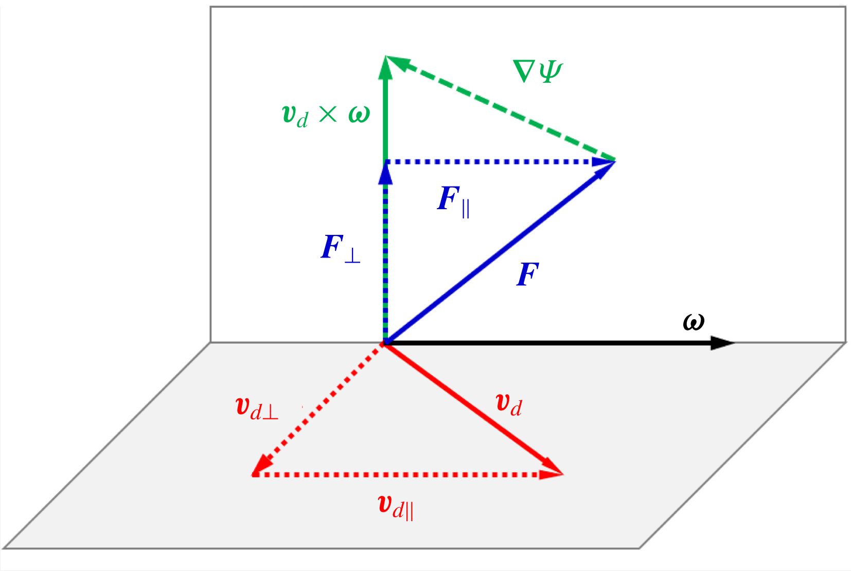
where $\boldsymbol{v}_{d}\equiv \boldsymbol{v}-\boldsymbol{u}$ denotes a drift velocity and $\unicode[STIX]{x1D6F9}$ is an arbitrary gauge. As sketched in figure 1, we introduce a vorticity-based orthogonal decomposition

(2.22) $$\begin{eqnarray}\boldsymbol{v}_{d}=\boldsymbol{v}_{d\bot }+\boldsymbol{v}_{d\Vert },\end{eqnarray}$$

where $\boldsymbol{v}_{d\bot }$ and $\boldsymbol{v}_{d\Vert }$ are respectively perpendicular and parallel to  $\unicode[STIX]{x1D74E}$ , and we can only determine $\boldsymbol{v}_{d\bot }$ from (2.21). The parallel component

(2.23) $$\begin{eqnarray}\boldsymbol{v}_{d\Vert }=C_{\Vert }\unicode[STIX]{x1D74E}\end{eqnarray}$$

with a constant or scalar function $C_{\Vert }$ can be arbitrary owing to $\boldsymbol{v}_{d\Vert }\times \unicode[STIX]{x1D74E}=0$ in (2.7).

Figure 1.

Diagram of the vorticity-based orthogonal decompositions of the non-ideal force and the virtual velocity.

By taking the cross-product of $\unicode[STIX]{x1D74E}$ with (2.21), we obtain

(2.24) $$\begin{eqnarray}\boldsymbol{v}_{d\bot }={\displaystyle \frac{\unicode[STIX]{x1D74E}\times (\boldsymbol{F}+\unicode[STIX]{x1D735}\unicode[STIX]{x1D6F9})}{\unicode[STIX]{x1D714}^{2}}},\end{eqnarray}$$

where $\unicode[STIX]{x1D714}\equiv |\unicode[STIX]{x1D74E}|$ is the magnitude of vorticity, and by taking the inner product of $\unicode[STIX]{x1D74E}$ with (2.21), $\unicode[STIX]{x1D6F9}$ in (2.24) satisfies

(2.25) $$\begin{eqnarray}\boldsymbol{F}\boldsymbol{\cdot }\unicode[STIX]{x1D74E}=-\unicode[STIX]{x1D74E}\boldsymbol{\cdot }\unicode[STIX]{x1D735}\unicode[STIX]{x1D6F9}.\end{eqnarray}$$

From (2.22) and (2.24), the virtual velocity is

(2.26) $$\begin{eqnarray}\boldsymbol{v}=\boldsymbol{u}+{\displaystyle \frac{\unicode[STIX]{x1D74E}\times (\boldsymbol{F}+\unicode[STIX]{x1D735}\unicode[STIX]{x1D6F9})}{\unicode[STIX]{x1D714}^{2}}}+C_{\Vert }\unicode[STIX]{x1D74E},\end{eqnarray}$$

which is in general not divergence-free. Appendix A.1 provides an example of the virtual velocity and illustrates its physical meaning in a two-dimensional TG flow.

It is noted that (2.25) can be satisfied locally (Greene Reference Greene1993), but a necessary condition for the existence and uniqueness of globally smooth solutions to the first-order partial differential equation of the type (2.25) with various boundary conditions is generally not clear. For example, the analysis of Huang, Küpper & Masbaum (Reference Huang, Küpper and Masbaum1997) showed that the existence and uniqueness of solutions to (2.25) with periodic conditions are not satisfied.

2.4 Existence and uniqueness of the virtual velocity

Since the existence and uniqueness of an explicit and globally smooth solution of $\boldsymbol{v}$ are not ensured in general non-ideal flows, we have to seek explicit $\boldsymbol{v}$ in the flows with special non-ideal forces. As sketched in figure 1, we apply the vorticity-based orthogonal decomposition to the non-ideal force in (2.2) as

(2.27) $$\begin{eqnarray}\boldsymbol{F}=\boldsymbol{F}_{\bot }+\boldsymbol{F}_{\Vert },\end{eqnarray}$$

where

(2.28) $$\begin{eqnarray}\boldsymbol{F}_{\bot }=\boldsymbol{F}-\frac{\boldsymbol{F}\boldsymbol{\cdot }\unicode[STIX]{x1D74E}}{\unicode[STIX]{x1D714}^{2}}\unicode[STIX]{x1D74E}\end{eqnarray}$$

is the component of $\boldsymbol{F}$ perpendicular to $\unicode[STIX]{x1D74E}$ and $\boldsymbol{F}_{\Vert }$ is the vorticity-parallel component. We remark that the decomposition is meaningless and the virtual velocity becomes singular at the points with $\unicode[STIX]{x1D714}=0$ , i.e. vorticity nulls or ‘vortex nulls’ (Saffman Reference Saffman1992).

Owing to the difficulty of determining $\unicode[STIX]{x1D6F9}$ from (2.25), we suppose that, in some particular cases, $\boldsymbol{F}_{\Vert }$ is irrotational or there exists a globally smooth $\unicode[STIX]{x1D6F9}$ satisfying

(2.29) $$\begin{eqnarray}\boldsymbol{F}_{\Vert }=-\unicode[STIX]{x1D735}\unicode[STIX]{x1D6F9}.\end{eqnarray}$$

As illustrated in figure 1, this choice has minimum $|\unicode[STIX]{x1D735}\unicode[STIX]{x1D6F9}|$ in all the possible $\unicode[STIX]{x1D735}\unicode[STIX]{x1D6F9}$ . Thus from (2.24) we can exactly determine

(2.30) $$\begin{eqnarray}\boldsymbol{v}_{d\bot }={\displaystyle \frac{\unicode[STIX]{x1D74E}\times \boldsymbol{F}_{\bot }}{\unicode[STIX]{x1D714}^{2}}}.\end{eqnarray}$$

A special case of (2.29) is $\boldsymbol{F}_{\Vert }=0$ , and (2.25) becomes

(2.31) $$\begin{eqnarray}\boldsymbol{F}\boldsymbol{\cdot }\unicode[STIX]{x1D74E}=0.\end{eqnarray}$$

We remark that

(2.32) $$\begin{eqnarray}\unicode[STIX]{x1D735}\times \boldsymbol{F}_{\Vert }=0\end{eqnarray}$$

is a sufficient condition for the existence of non-trivial smooth $\boldsymbol{v}$ at the points with $\unicode[STIX]{x1D714}\neq 0$ . Appendix A.2 provides an example of an exact solution of $\boldsymbol{v}$ with $\unicode[STIX]{x1D735}\times \boldsymbol{F}_{\Vert }\neq 0$ in an integrable Arnold–Beltrami–Childress (ABC) flow.

If there exist globally smooth solutions of $\boldsymbol{v}_{d}$ , we need additional constraints to determine a unique virtual velocity. First, the choice of $\boldsymbol{v}_{\Vert }$ in (2.26) does not affect vorticity transport in (2.8), so we can choose $C_{\Vert }=0$ in (2.26) without loss of generality. Second, if the solution of $\unicode[STIX]{x1D6F9}$ for (2.25) exists but is not unique, we propose an additional constraint

(2.33) $$\begin{eqnarray}\min \langle |\unicode[STIX]{x1D735}\unicode[STIX]{x1D6F9}|\rangle\end{eqnarray}$$

to determine unique $\unicode[STIX]{x1D735}\unicode[STIX]{x1D6F9}$ , where $\langle \cdot \rangle$ denotes the volume average. This constraint makes the virtual velocity finite and smooth, and it is consistent with (2.29) under condition (2.32). Taking a two-dimensional flow for example, we obtain $\boldsymbol{v}_{d}=-\unicode[STIX]{x1D708}\unicode[STIX]{x1D735}\unicode[STIX]{x1D714}/\unicode[STIX]{x1D714}$ from (2.30) with $\boldsymbol{F}_{\Vert }=0$ . Moreover, it is possible to calculate an approximate virtual velocity using numerical methods, which is out of scope of the present study.

2.5 Virtual velocity in modified fluid flows

Given the difficulty for determining a globally smooth virtual velocity in real flows, we propose a modified fluid flow in which explicit $\boldsymbol{v}$ can be obtained. This modified flow is artificial and only used for the theoretical study of accurately tracking vortex surfaces.

For simplicity, we consider an incompressible barotropic viscous flow governed by

(2.34) $$\begin{eqnarray}\left.\begin{array}{@{}c@{}}{\displaystyle \frac{\unicode[STIX]{x2202}\boldsymbol{u}}{\unicode[STIX]{x2202}t}}+\boldsymbol{u}\boldsymbol{\cdot }\unicode[STIX]{x1D735}\boldsymbol{u}=-{\displaystyle \frac{1}{\unicode[STIX]{x1D70C}}}\unicode[STIX]{x1D735}p+\boldsymbol{F},\\ \unicode[STIX]{x1D735}\boldsymbol{\cdot }\boldsymbol{ u}=0.\end{array}\right\}\end{eqnarray}$$

The requirement (2.32) can be satisfied by imposing $\boldsymbol{F}_{\Vert }=0$ . Thus we obtain a modified NS (MNS) equation:

(2.35) $$\begin{eqnarray}{\displaystyle \frac{\unicode[STIX]{x2202}\boldsymbol{u}}{\unicode[STIX]{x2202}t}}+\boldsymbol{u}\boldsymbol{\cdot }\unicode[STIX]{x1D735}\boldsymbol{u}=-\frac{1}{\unicode[STIX]{x1D70C}}\unicode[STIX]{x1D735}p+\boldsymbol{F}_{\bot }.\end{eqnarray}$$

This equation can be valid in some real flows, e.g. two-dimensional flows, or in a modified flow with a special constitutive relation. Then the vorticity equation becomes

(2.36) $$\begin{eqnarray}\frac{\unicode[STIX]{x2202}\unicode[STIX]{x1D74E}}{\unicode[STIX]{x2202}t}=\unicode[STIX]{x1D735}\times (\boldsymbol{u}\times \unicode[STIX]{x1D74E})+\unicode[STIX]{x1D735}\times \boldsymbol{F}_{\bot }.\end{eqnarray}$$

For the MNS equation, we set $\unicode[STIX]{x1D6F9}=0$ based on (2.33) and $C_{\Vert }=0$ in (2.23), then we uniquely determine the virtual velocity (2.26) as

(2.37) $$\begin{eqnarray}\boldsymbol{v}=\boldsymbol{u}+\frac{\unicode[STIX]{x1D74E}\times \boldsymbol{F}_{\bot }}{\unicode[STIX]{x1D714}^{2}}.\end{eqnarray}$$

The modified flow governed by (2.35) has virtual Kelvin’s theorem and other virtual vorticity conservation theorems in § 2.2 except at vorticity nulls. Thus the virtual evolution of vortex lines or surfaces can be topologically invariant in the modified dissipative flow. Here, we only consider a modified viscous term in $\boldsymbol{F}_{\bot }$ as

(2.38) $$\begin{eqnarray}\boldsymbol{F}_{\bot }=\unicode[STIX]{x1D708}\left[\unicode[STIX]{x1D6FB}^{2}\boldsymbol{u}-\frac{(\unicode[STIX]{x1D6FB}^{2}\boldsymbol{u}\boldsymbol{\cdot }\unicode[STIX]{x1D74E})\unicode[STIX]{x1D74E}}{\unicode[STIX]{x1D714}^{2}}\right].\end{eqnarray}$$

The corresponding drift velocity (2.37) becomes

(2.39) $$\begin{eqnarray}\boldsymbol{v}_{d}=\unicode[STIX]{x1D708}\frac{(\unicode[STIX]{x1D735}\times \unicode[STIX]{x1D74E})\times \unicode[STIX]{x1D74E}}{\unicode[STIX]{x1D714}^{2}}=-\unicode[STIX]{x1D708}\frac{\unicode[STIX]{x1D735}\unicode[STIX]{x1D714}}{\unicode[STIX]{x1D714}}+\unicode[STIX]{x1D708}\frac{(\unicode[STIX]{x1D74E}\boldsymbol{\cdot }\unicode[STIX]{x1D735})\unicode[STIX]{x1D74E}}{\unicode[STIX]{x1D714}^{2}},\end{eqnarray}$$

where the first term on the right-hand side denotes a velocity pointing from high- $\unicode[STIX]{x1D714}$ region to low- $\unicode[STIX]{x1D714}$ region, and the second term appears to be highly nonlinear in three-dimensional flows and it vanishes in two-dimensional flows.

The transport equation for the enstrophy $\unicode[STIX]{x1D6FA}\equiv \unicode[STIX]{x1D714}^{2}/2$ in the modified fluid is derived from (2.36) as

(2.40) $$\begin{eqnarray}\frac{\text{D}\unicode[STIX]{x1D6FA}}{\text{D}t}=\unicode[STIX]{x1D74E}\boldsymbol{\cdot }\unicode[STIX]{x1D64E}\boldsymbol{\cdot }\unicode[STIX]{x1D74E}+\unicode[STIX]{x1D74E}\boldsymbol{\cdot }(\unicode[STIX]{x1D735}\times \boldsymbol{F}_{\bot }),\end{eqnarray}$$

where $\unicode[STIX]{x1D64E}\equiv (\unicode[STIX]{x1D735}\boldsymbol{u}+\unicode[STIX]{x1D735}\boldsymbol{u}^{T})/2$ is the rate-of-strain tensor. Substituting (2.38) into (2.40) yields

(2.41) $$\begin{eqnarray}\frac{\text{D}\unicode[STIX]{x1D6FA}}{\text{D}t}=\unicode[STIX]{x1D74E}\boldsymbol{\cdot }\unicode[STIX]{x1D64E}\boldsymbol{\cdot }\unicode[STIX]{x1D74E}+\unicode[STIX]{x1D708}\{-(\sin ^{2}\unicode[STIX]{x1D717}_{\unicode[STIX]{x1D714}})(\unicode[STIX]{x1D6FB}^{2}\boldsymbol{u})^{2}+\unicode[STIX]{x1D735}\boldsymbol{\cdot }[\unicode[STIX]{x1D74E}\times (\unicode[STIX]{x1D735}\times \unicode[STIX]{x1D74E})]\}\end{eqnarray}$$

after some algebra, where $\unicode[STIX]{x1D717}_{\unicode[STIX]{x1D714}}$ denotes the angle between $\unicode[STIX]{x1D74E}$ and $\unicode[STIX]{x1D6FB}^{2}\boldsymbol{u}$ . Comparing (2.41) and the enstrophy equation (see Davidson Reference Davidson2004)

(2.42) $$\begin{eqnarray}\frac{\text{D}\unicode[STIX]{x1D6FA}}{\text{D}t}=\unicode[STIX]{x1D74E}\boldsymbol{\cdot }\unicode[STIX]{x1D64E}\boldsymbol{\cdot }\unicode[STIX]{x1D74E}+\unicode[STIX]{x1D708}\{-(\unicode[STIX]{x1D6FB}^{2}\boldsymbol{u})^{2}+\unicode[STIX]{x1D735}\boldsymbol{\cdot }[\unicode[STIX]{x1D74E}\times (\unicode[STIX]{x1D735}\times \unicode[STIX]{x1D74E})]\}\end{eqnarray}$$

for real fluid flows with the NS equation (2.2), we find that the prefactor $0\leqslant \sin ^{2}\unicode[STIX]{x1D717}_{\unicode[STIX]{x1D714}}\leqslant 1$ of the second term on the right-hand side of (2.41) weakens the enstrophy dissipation term in the modified fluid flow without the vorticity-parallel component of the viscous term in the MNS equation (2.35). Thus this modified fluid flow is dissipative, but less dissipative than real flows.

As another example of the modified fluid, in the framework of incompressible Schrödinger flow (ISF) (Chern et al. Reference Chern, Knöppel, Pinkall, Schröder and Weißmann2016), the ideal flow is modified by a ‘Landau–Lifshitz term’ which shares some physical features in superfluids. As discussed in § A.3, we find that this non-ideal term is also orthogonal to the vorticity, so it can be included in the drift velocity. Chern (Reference Chern2017) argued that the drift velocity (also referred to as ‘Landau–Lifshitz velocity’ in ISF) regularizes the Euler equation and enhances additional localized induction of vortex filaments.

3.1 Original formulation of the VSF

The VSF is a Lagrangian-based structure identification method rooted in Helmholtz’s theorem. The VSF is defined as a smooth scalar field satisfying the constraint (see Yang & Pullin Reference Yang and Pullin2010)

(3.1) $$\begin{eqnarray}\unicode[STIX]{x1D74E}\boldsymbol{\cdot }\unicode[STIX]{x1D735}\unicode[STIX]{x1D719}_{v}=0,\end{eqnarray}$$

so that $\unicode[STIX]{x1D74E}$ is tangent at every point on an isosurface of  $\unicode[STIX]{x1D719}_{v}$ . Namely, each VSF isosurface is a vortex surface consisting of vortex lines.

In order to characterize the temporal evolution of VSFs, we seek $\unicode[STIX]{x1D719}_{v}(\boldsymbol{x},t)$ satisfying constraint (3.1) at all time as

(3.2) $$\begin{eqnarray}{\displaystyle \frac{\text{D}}{\text{D}t}}(\unicode[STIX]{x1D74E}\boldsymbol{\cdot }\unicode[STIX]{x1D735}\unicode[STIX]{x1D719}_{v})=0.\end{eqnarray}$$

Similar to the derivation in Yang & Pullin (Reference Yang and Pullin2010), we derive the evolution equation for the VSF from (2.4) and (3.2) as

(3.3) $$\begin{eqnarray}{\displaystyle \frac{\text{D}\unicode[STIX]{x1D719}_{v}}{\text{D}t}}=\mathscr{L},\end{eqnarray}$$

with

(3.4) $$\begin{eqnarray}\unicode[STIX]{x1D735}\unicode[STIX]{x1D719}_{v}\boldsymbol{\cdot }(\unicode[STIX]{x1D735}\times \boldsymbol{F})+\unicode[STIX]{x1D74E}\boldsymbol{\cdot }\unicode[STIX]{x1D735}\mathscr{L}-(\unicode[STIX]{x1D735}\boldsymbol{\cdot }\boldsymbol{v})\unicode[STIX]{x1D74E}\boldsymbol{\cdot }\unicode[STIX]{x1D735}\unicode[STIX]{x1D719}_{v}=0,\end{eqnarray}$$

where $\mathscr{L}$ is a scalar field and represents the effects of non-ideal forces on the evolution of VSF.

Similar to the difficulty of (2.25) in determining the virtual velocity, the existence and uniqueness of solutions to the first-order partial differential equation (3.4) for $\mathscr{L}$ are also an open problem. A two-time method is developed to numerically solve (3.3) and (3.4) by introducing a dissipative numerical regularization (Yang & Pullin Reference Yang and Pullin2011). Although the numerical method has been successfully applied to highly symmetric flows and transitional channel flows (Zhao et al. Reference Zhao, Yang and Chen2016), the numerical regularization still has the uniqueness issue of VSF solutions.

3.2 Transport of the VSF in the virtual velocity

Based on the virtual velocity, we reformulate transport equations of the VSF in non-ideal flows. If $\unicode[STIX]{x1D719}_{v}$ is a VSF at an initial time and it evolves as $\text{D}\unicode[STIX]{x1D719}_{v}/\text{D}t=0$ , it is always a VSF satisfying (3.2) at all time in ideal flows from Ertel’s theorem. Although this frozen-in nature of VSF breaks down in non-ideal flows, the form of (3.2) can be still valid in the virtual velocity.

Considering $\unicode[STIX]{x1D719}_{v}$ is convected along a globally smooth virtual velocity as

(3.5) $$\begin{eqnarray}{\displaystyle \frac{\text{D}_{v}\unicode[STIX]{x1D719}_{v}}{\text{D}_{v}t}}=0,\end{eqnarray}$$

with a VSF initial condition, from (2.18) in virtual Ertel’s theorem without considering  $\unicode[STIX]{x1D70C}$ , we have

(3.6) $$\begin{eqnarray}{\displaystyle \frac{\text{D}_{v}}{\text{D}_{v}t}}(\unicode[STIX]{x1D74E}\boldsymbol{\cdot }\unicode[STIX]{x1D735}\unicode[STIX]{x1D719}_{v})=0.\end{eqnarray}$$

Thus we can exactly track the VSF from (3.5) from the virtual Lagrangian view.

Figure 2.

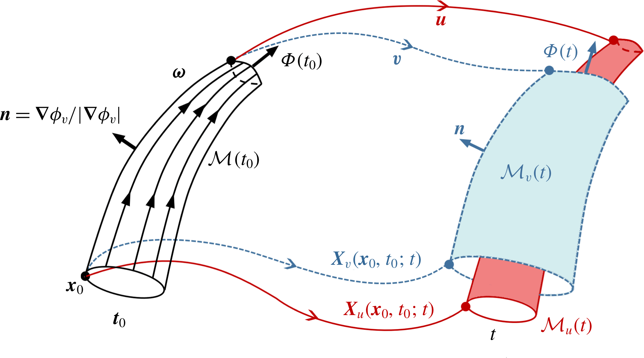
Sketch of the surface evolution convected by the virtual or physical velocity in a non-ideal flow. At time  $t_{0}$ , the black solid surface denotes the initial vortex tube ${\mathcal{M}}(t_{0})$ with vortex lines (black lines with arrows), the surface normal $\boldsymbol{n}=\unicode[STIX]{x1D735}\unicode[STIX]{x1D719}_{v}/|\unicode[STIX]{x1D735}\unicode[STIX]{x1D719}_{v}|$ and the vorticity flux $\unicode[STIX]{x1D6F7}(t_{0})$ . At time $t$ , the blue surface ${\mathcal{M}}_{v}(t_{0})$ denotes the vortex surface convected by  $\boldsymbol{v}$ ; the red surface ${\mathcal{M}}_{u}(t_{0})$ denotes the material surface convected by  $\boldsymbol{u}$ . The dotted blue and solid red lines with arrows denote trajectories of $\boldsymbol{X}_{v}(\boldsymbol{x}_{0},t_{0};t)$ and $\boldsymbol{X}_{u}(\boldsymbol{x}_{0},t_{0};t)$ from the same initial position $\boldsymbol{x}_{0}$ but convected by $\boldsymbol{v}$ and  $\boldsymbol{u}$ , respectively.

The tracking of a vortex surface (or tube) frozen in the virtual velocity in a non-ideal flow is sketched in figure 2, and the tracking of a material surface from the same initial surface is also shown for comparison. From the Lagrangian view, the surface tracking in the narrow sense is described by the flow map of a surface. Evolving from the same vortex surface ${\mathcal{M}}(t_{0})$ at initial time  $t_{0}$ ,

(3.7a,b ) $$\begin{eqnarray}{\mathcal{M}}_{v}(t):={\mathcal{F}}_{t_{0},v}^{t}({\mathcal{M}}(t_{0}))\quad \text{and}\quad {\mathcal{M}}_{u}(t):={\mathcal{F}}_{t_{0},u}^{t}({\mathcal{M}}(t_{0}))\end{eqnarray}$$

denote the vortex surface convected by $\boldsymbol{v}$ and the material surface convected by  $\boldsymbol{u}$ , respectively, where the flow maps are defined as

(3.8a,b ) $$\begin{eqnarray}{\mathcal{F}}_{t_{0},v}^{t}(\boldsymbol{x}_{0}):=\boldsymbol{X}_{v}(\boldsymbol{x}_{0},t_{0};t)\quad \text{and}\quad {\mathcal{F}}_{t_{0},u}^{t}(\boldsymbol{x}_{0}):=\boldsymbol{X}_{u}(\boldsymbol{x}_{0},t_{0};t).\end{eqnarray}$$

Here, the Lagrangian coordinates $\boldsymbol{X}_{v}(\boldsymbol{x}_{0},t_{0};t)$ convected by $\boldsymbol{v}$ and $\boldsymbol{X}_{u}(\boldsymbol{x}_{0},t_{0};t)$ convected by $\boldsymbol{u}$ are governed by

(3.9a,b ) $$\begin{eqnarray}\frac{\text{D}\boldsymbol{X}_{v}}{\text{D}t}=\boldsymbol{v}(\boldsymbol{X}_{v},t)\quad \text{and}\quad \frac{\text{D}\boldsymbol{X}_{u}}{\text{D}t}=\boldsymbol{u}(\boldsymbol{X}_{u},t),\end{eqnarray}$$

respectively, and the coordinates are labelled at the same initial position  $\boldsymbol{x}_{0}$ .

In terms of the VSF, the vortex surface is an isosurface of $\unicode[STIX]{x1D719}_{v}$ at a particular isocontour value, where $\unicode[STIX]{x1D719}_{v}$ is governed by (3.5). The vorticity flux $\unicode[STIX]{x1D6F7}(t)$ through a cross-section of vortex tube ${\mathcal{M}}_{v}(t)$ is conserved from (2.12) in virtual Helmholtz’s theorem. The surfaces ${\mathcal{M}}_{v}(t)$ and ${\mathcal{M}}_{u}(t)$ are the same in ideal flows, whereas they are different in non-ideal flows. As discussed in § A.1 and illustrated in figure 2, the viscous effect can diminish the vorticity flux, so the radius of the vortex tube ${\mathcal{M}}_{v}(t)$ can be larger than that of the material one ${\mathcal{M}}_{v}(t)$ to keep vorticity flux $\unicode[STIX]{x1D6F7}(t)=\unicode[STIX]{x1D6F7}(t_{0})$ invariant.

Furthermore, the helicity is conserved in ideal flows, but not conserved in non-ideal flows, i.e. vortex lines or surfaces can have reconnection. From (2.19) in the virtual helicity conservation theorem, the helicity is still conserved in a virtual material volume convected along the virtual velocity. This implies that topological properties of vortex lines within a virtual material volume are invariant, and this topological invariance breaks down at vorticity nulls owing to the singular virtual velocity.

Although both VSF formulations (3.3) and (3.5) have the common difficulty on solving first-order partial differential equations, the VSF formulation with the virtual velocity provides a physical explanation of the VSF transport in non-ideal flows. If a globally smooth virtual velocity exists, the VSF isosurface is the carrier for Theorems 2–4, which will be discussed in § 5. If not, an approximate virtual velocity can be still useful to reduce the deviation from the virtual conservation theorems in VSF calculation, which will be discussed in § 6.

4.1 DNS of HD TG flows

The DNS of HD flows is used to solve the incompressible NS equation (2.34) with $\boldsymbol{F}=\unicode[STIX]{x1D708}\unicode[STIX]{x1D6FB}^{2}\boldsymbol{u}$ and the MNS equation (2.35) with $\boldsymbol{F}_{\bot }$ (2.38) in a periodic cube of side $2\unicode[STIX]{x03C0}$ . The HD TG flow evolution from the TG initial condition (Taylor & Green Reference Taylor and Green1937)

(4.1) $$\begin{eqnarray}\boldsymbol{u}_{0}=(\sin x\cos y\cos z,-\cos x\sin y\cos z,0)\end{eqnarray}$$

has a transitional process with the rapid development of small-scale vortical structures as energy cascade. Within the periodic cube, there are multiple mirror symmetries, anti-symmetries and rotational symmetries with fixed vorticity nulls at the intersections of symmetric planes (see Brachet et al. Reference Brachet, Meiron, Orszag, Nickel, Morf and Frisch1983). These symmetries were utilized to reduce the computational cost for calculating the evolution of VSFs.

The DNS was carried out using the standard pseudo-spectral method on uniform grid points $N^{3}=512^{3}$ at the Reynolds number $Re\equiv 1/\unicode[STIX]{x1D708}=100$ . The spatial resolution is high enough for the TG flow at such a low $Re$ (Brachet et al. Reference Brachet, Meiron, Orszag, Nickel, Morf and Frisch1983). Aliasing errors were removed using the two-thirds dealiasing rule with the maximum wavenumber $k_{max}=N/3$ . The temporal integration of the Fourier coefficients of $\boldsymbol{u}$ was performed using a second-order Runge–Kutta scheme. The time step $\unicode[STIX]{x0394}t$ was selected to ensure that the Courant–Friedrichs–Lewy (CFL) number

(4.2) $$\begin{eqnarray}\text{CFL}=\frac{\unicode[STIX]{x0394}t}{\unicode[STIX]{x0394}x}\max (|u_{x}|,|u_{y}|,|u_{z}|)\end{eqnarray}$$

is less than 0.5 for numerical stability and accuracy, where $\unicode[STIX]{x0394}x=2\unicode[STIX]{x03C0}/N$ denotes the grid spacing. Moreover, the singular modified viscous term (2.38) at vorticity nulls was smoothed by multiplying a smoothing coefficient $C_{\unicode[STIX]{x1D716}}=\unicode[STIX]{x1D714}^{2}/(\unicode[STIX]{x1D714}^{2}+\unicode[STIX]{x1D716})$ in the MNS equation (2.35) with $\unicode[STIX]{x1D716}=1\times 10^{-6}$ .

4.2 DNS of MHD TG flows

The incompressible MHD equations in terms of dimensionless velocity $\boldsymbol{u}$ and magnetic induction $\boldsymbol{b}$ read (e.g. see Priest & Forbes Reference Priest and Forbes2000)

(4.3) $$\begin{eqnarray}\left.\begin{array}{@{}c@{}}{\displaystyle \frac{\unicode[STIX]{x2202}\boldsymbol{u}}{\unicode[STIX]{x2202}t}}+\boldsymbol{u}\boldsymbol{\cdot }\unicode[STIX]{x1D735}\boldsymbol{u}=-{\displaystyle \frac{1}{\unicode[STIX]{x1D70C}}}\unicode[STIX]{x1D735}p+\boldsymbol{j}\times \boldsymbol{b}+\unicode[STIX]{x1D708}\unicode[STIX]{x1D6FB}^{2}\boldsymbol{u},\\ {\displaystyle \frac{\unicode[STIX]{x2202}\boldsymbol{b}}{\unicode[STIX]{x2202}t}}=\unicode[STIX]{x1D735}\times (\boldsymbol{u}\times \boldsymbol{b})+\unicode[STIX]{x1D702}\unicode[STIX]{x1D6FB}^{2}\boldsymbol{b},\end{array}\right\}\end{eqnarray}$$

together with $\unicode[STIX]{x1D735}\boldsymbol{\cdot }\boldsymbol{u}=0$ and $\unicode[STIX]{x1D735}\boldsymbol{\cdot }\boldsymbol{b}=0$ , where $\unicode[STIX]{x1D702}$ denotes the magnetic diffusivity and $\boldsymbol{j}=\unicode[STIX]{x1D735}\times \boldsymbol{b}$ the current density. We define the magnetic Reynolds number $Rm=1/\unicode[STIX]{x1D702}$ , and assume that the MHD flows in DNS have the unity magnetic Prandtl number with $Re=Rm$ .

The same TG initial velocity (4.1) is applied in the DNS of MHD flows. Additionally, two TG-type initial magnetic fields are considered. The first one is the steady initial condition with $\boldsymbol{b}_{0}=\boldsymbol{u}_{0}$ . For this steady case, MHD equations (4.3) degenerate into pure diffusion equations

(4.4a,b ) $$\begin{eqnarray}{\displaystyle \frac{\unicode[STIX]{x2202}\unicode[STIX]{x1D74E}}{\unicode[STIX]{x2202}t}}=\unicode[STIX]{x1D708}\unicode[STIX]{x1D6FB}^{2}\unicode[STIX]{x1D74E}\quad \text{and}\quad {\displaystyle \frac{\unicode[STIX]{x2202}\boldsymbol{b}}{\unicode[STIX]{x2202}t}}=\unicode[STIX]{x1D702}\unicode[STIX]{x1D6FB}^{2}\boldsymbol{b}.\end{eqnarray}$$

The second initial magnetic field is the ‘insulating’ condition (see Lee et al. Reference Lee, Brachet, Pouquet, Rosenberg and Mininni2009)

(4.5) $$\begin{eqnarray}\boldsymbol{b}_{0}=b_{0}(\cos x\sin y\sin z,\sin x\cos y\sin z,-2\sin x\sin y\cos z),\end{eqnarray}$$

with $b_{0}=1/\sqrt{3}$ . For this initial condition, the current $\boldsymbol{j}$ is contained within each ‘insulating box’, e.g.  $[0,\unicode[STIX]{x03C0}]^{3}$ , and $\boldsymbol{b}$ is proportional to $\unicode[STIX]{x1D74E}$ at the initial time.

As in the DNS of HD flows, the DNS of MHD flows was also carried out on uniform grid points $N^{3}=512^{3}$ in a periodic cube with side $2\unicode[STIX]{x03C0}$ . A symmetric form of (4.3) with the Elsässer variables $\boldsymbol{z}^{\pm }=\boldsymbol{u}\pm \boldsymbol{b}$ (see Elsässer Reference Elsässer1950) is solved using the pseudo-spectral method (see Aluie Reference Aluie2009). The two-thirds dealiasing rule was applied and the temporal integration was performed using a second-order Runge–Kutta scheme.

4.3 Calculation of VSFs

First, initial VSF $\unicode[STIX]{x1D719}_{v0}$ is constructed to satisfy the VSF constraint (3.1). For the TG initial velocity (4.1), the initial VSF is

(4.6) $$\begin{eqnarray}\unicode[STIX]{x1D719}_{v0}=(\cos 2x-\cos 2y)\cos z.\end{eqnarray}$$

Then the evolution of the VSF is calculated using the two-time method (Yang & Pullin Reference Yang and Pullin2011). Each time step is divided into prediction and correction sub-steps. In the prediction sub-step, the temporary VSF $\unicode[STIX]{x1D719}_{v}^{\ast }$ is driven by an advection velocity $\boldsymbol{V}$ as

(4.7) $$\begin{eqnarray}\frac{\unicode[STIX]{x2202}\unicode[STIX]{x1D719}_{v}^{\ast }(\boldsymbol{x},t)}{\unicode[STIX]{x2202}t}+\boldsymbol{V}(\boldsymbol{x},t)\boldsymbol{\cdot }\unicode[STIX]{x1D735}\unicode[STIX]{x1D719}_{v}^{\ast }(\boldsymbol{x},t)=0,\quad t>0.\end{eqnarray}$$

In the correction sub-step, $\unicode[STIX]{x1D719}_{v}^{\ast }$ is driven by the frozen vorticity at a fixed physical time $t$ and evolved in pseudo time $\unicode[STIX]{x1D70F}$ as

(4.8) $$\begin{eqnarray}\frac{\unicode[STIX]{x2202}\unicode[STIX]{x1D719}_{v}^{\ast }(\boldsymbol{x},t;\unicode[STIX]{x1D70F})}{\unicode[STIX]{x2202}t}+\unicode[STIX]{x1D74E}(\boldsymbol{x},t)\boldsymbol{\cdot }\unicode[STIX]{x1D735}\unicode[STIX]{x1D719}_{v}^{\ast }(\boldsymbol{x},t;\unicode[STIX]{x1D70F})=0,\quad 0<\unicode[STIX]{x1D70F}\leqslant T_{\unicode[STIX]{x1D70F}},\end{eqnarray}$$

where the initial condition is $\unicode[STIX]{x1D719}_{v}(\boldsymbol{x},t;\unicode[STIX]{x1D70F}=0)=\unicode[STIX]{x1D719}_{v}^{\ast }(\boldsymbol{x},t)$ . At the end of the correction sub-step, $\unicode[STIX]{x1D719}_{v}$ is updated by $\unicode[STIX]{x1D719}_{v}^{\ast }(\boldsymbol{x},t;\unicode[STIX]{x1D70F}=T_{\unicode[STIX]{x1D70F}})$ , where $T_{\unicode[STIX]{x1D70F}}$ is the maximum pseudo time and is typically less than 100 times $\unicode[STIX]{x0394}t$ .

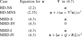
Different choices of $\boldsymbol{V}$ in (4.7), either the physical velocity for solving (3.3) or the virtual velocity for solving (3.5), are applied for different DNS cases, and they are summarized in table 1. If $\boldsymbol{V}$ is a physical velocity, the temporary $\unicode[STIX]{x1D719}_{v}^{\ast }$ deviates from an accurate VSF owing to the breakdown of Helmholtz’s theorem in non-ideal flows. In the correction sub-step, the temporary $\unicode[STIX]{x1D719}_{v}^{\ast }$ in the VSF evolution is convected along the frozen vorticity in (4.8), which projects $\unicode[STIX]{x1D719}_{v}^{\ast }$ onto the desired VSF solution. If $\boldsymbol{V}$ is a virtual velocity, the correction sub-step only serves as a further numerical correction for preserving the isosurfaces of $\unicode[STIX]{x1D719}_{v}$ as vortex surfaces.

Table 1.

Set-up of different DNS cases and corresponding VSF calculations.

The numerical schemes for solving (4.7) and (4.8) are described in detail in Yang & Pullin (Reference Yang and Pullin2011). Temporal integrations are marched by the third-order total-variation-diminishing Runge–Kutta scheme (see Gottlieb & Shu Reference Gottlieb and Shu1998). The time steps $\unicode[STIX]{x0394}t$ and $\unicode[STIX]{x0394}\unicode[STIX]{x1D70F}$ were chosen to ensure the corresponding CFL conditions based on $\boldsymbol{V}$ and  $\unicode[STIX]{x1D74E}$ , respectively. The convection terms were treated by the fifth-order weighted essentially non-oscillatory (WENO) scheme (see Jiang & Shu Reference Jiang and Shu1996) and the numerical diffusion in the WENO scheme serves as a numerical dissipative regularization for removing small-scale, nearly singular scalar structures. The computational domain for the VSF calculation was selected as $\boldsymbol{x}\in [0,\unicode[STIX]{x03C0}/2]\times [0,\unicode[STIX]{x03C0}/2]\times [\unicode[STIX]{x03C0}/2,\unicode[STIX]{x03C0}]$ . The periodic condition and other boundary conditions under TG symmetries (see Yang & Pullin Reference Yang and Pullin2010) were applied. The grid resolution for the VSF in the periodic cube is $N^{3}=512^{3}$ , the same as that for the velocity field in both HD and MHD flows. Additionally, the singular drift velocity at vorticity nulls in case MHD-IV was smoothed as $C_{\unicode[STIX]{x1D716}}\boldsymbol{v}_{d}$ .

In practice, the computed $\unicode[STIX]{x1D719}_{v}$ can have a small deviation from an exact VSF owing to the numerical regularization. The VSF deviation (see Yang & Pullin Reference Yang and Pullin2010) is quantified by the cosine of the angle between the vorticity field $\unicode[STIX]{x1D74E}$ and the gradient of VSF $\unicode[STIX]{x1D735}\unicode[STIX]{x1D719}_{v}$ as

(4.9) $$\begin{eqnarray}\unicode[STIX]{x1D706}_{\unicode[STIX]{x1D714}}=\frac{\unicode[STIX]{x1D74E}\boldsymbol{\cdot }\unicode[STIX]{x1D735}\unicode[STIX]{x1D719}_{v}}{|\unicode[STIX]{x1D74E}|\,|\unicode[STIX]{x1D735}\unicode[STIX]{x1D719}_{v}|}.\end{eqnarray}$$

Thus an exact VSF solution has $\unicode[STIX]{x1D706}_{\unicode[STIX]{x1D714}}=0$ , and a relatively accurate numerical solution should have a small enough $\langle |\unicode[STIX]{x1D706}_{\unicode[STIX]{x1D714}}|\rangle$ so that we can extract isosurfaces of the VSF solution to study the evolution of vortex surfaces.

4.4 Error estimation for the approximated virtual velocity used in VSF calculation

Although conceptually the VSF can be tracked from the virtual Lagrangian view by setting the advection velocity as the virtual velocity in (3.5), the conditions for the existence and uniqueness of (2.30) are not ensured in general three-dimensional flows. For VSF calculation, if we use the explicit expression (2.37), which is only exact for the modified fluid flows with $\unicode[STIX]{x1D735}\times \boldsymbol{F}_{\Vert }\neq 0$ , to approximate the general virtual velocity (2.26) in (3.5), the deviation owing to the absence of $\unicode[STIX]{x1D735}\unicode[STIX]{x1D6F9}$ is defined as

(4.10) $$\begin{eqnarray}\unicode[STIX]{x1D716}_{\unicode[STIX]{x1D6F9}}\equiv \frac{(\unicode[STIX]{x1D74E}\times \unicode[STIX]{x1D735}\unicode[STIX]{x1D6F9})\boldsymbol{\cdot }\unicode[STIX]{x1D735}\unicode[STIX]{x1D719}_{v}}{\unicode[STIX]{x1D714}^{2}},\end{eqnarray}$$

with constraint equations (2.25) and (3.1).

Next we provide an order analysis of $\unicode[STIX]{x1D716}_{\unicode[STIX]{x1D6F9}}$ as an error estimation for the approximate virtual velocity (2.37) used in VSF calculation. Here, we assume $\boldsymbol{F}$ has a preferential normal alignment with $\unicode[STIX]{x1D74E}$ in a particular flow evolution, and then

(4.11) $$\begin{eqnarray}\unicode[STIX]{x1D74E}\boldsymbol{\cdot }\unicode[STIX]{x1D735}\unicode[STIX]{x1D6F9}=\unicode[STIX]{x1D6FF}_{F}\end{eqnarray}$$

is very small from (2.25). This assumption implies that

(4.12) $$\begin{eqnarray}|\unicode[STIX]{x1D735}\unicode[STIX]{x1D6F9}|=\frac{\unicode[STIX]{x1D6FF}_{F}}{\unicode[STIX]{x1D714}\cos \unicode[STIX]{x1D717}_{F}},\end{eqnarray}$$

where $\unicode[STIX]{x1D717}_{F}$ denotes the angle between $\boldsymbol{F}$ and $\unicode[STIX]{x1D74E}$ . Substituting (4.12) into (4.10) yields

(4.13) $$\begin{eqnarray}O(\unicode[STIX]{x1D716}_{\unicode[STIX]{x1D6F9}})\sim O\left(\frac{|\unicode[STIX]{x1D6FF}_{F}|\,|\unicode[STIX]{x1D735}\unicode[STIX]{x1D719}_{v}|\,|\text{tan}\,\unicode[STIX]{x1D717}_{F}|}{\unicode[STIX]{x1D714}^{2}}\right).\end{eqnarray}$$

Considering the uniqueness constraint (2.33), which is equivalent to $\max \langle |\text{cos}\,\unicode[STIX]{x1D717}_{F}|\rangle$ in (4.12) or $\min \langle |\text{tan}\,\unicode[STIX]{x1D717}_{F}|\rangle$ in (4.13), (4.13) becomes $O(\unicode[STIX]{x1D716}_{\unicode[STIX]{x1D6F9}})\sim O(|\unicode[STIX]{x1D6FF}_{F}|\,|\unicode[STIX]{x1D735}\unicode[STIX]{x1D719}_{v}|/\unicode[STIX]{x1D714}^{2})$ , and it can be small if we track the VSF frozen in (2.37) in the non-ideal flow with small  $\boldsymbol{F}_{\Vert }$ .

5.1 Statistics in real and modified flows

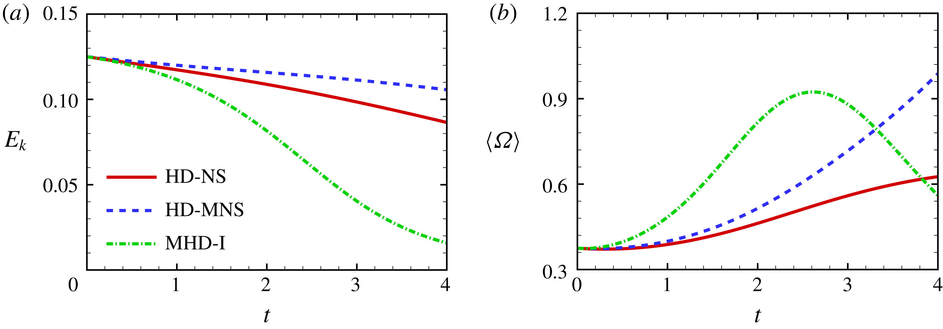
In order to investigate the influence of vorticity-parallel and vorticity-normal non-ideal force components on flow evolution, we carry out DNS cases HD-NS and HD-MNS (see table 1) at $Re=100$ . The temporal evolutions of the total kinetic energy $E_{k}\equiv \langle |\boldsymbol{u}|^{2}\rangle /2$ and enstrophy $\unicode[STIX]{x1D6FA}$ in the two cases are compared in figure 3. We find that the decay of $E_{k}$ in HD-MNS is slower than that in HD-NS, and $\langle \unicode[STIX]{x1D6FA}\rangle$ in HD-MNS is always larger than that in HD-NS. This observation agrees with the theoretical analysis by comparing (2.41) and (2.42), i.e. the modified fluid flow is less dissipative than the real fluid flow.

Figure 3.

Temporal evolution of the volume-averaged (a) total kinetic energy and (b) enstrophy in cases HD-NS, HD-MNS and MHD-I.

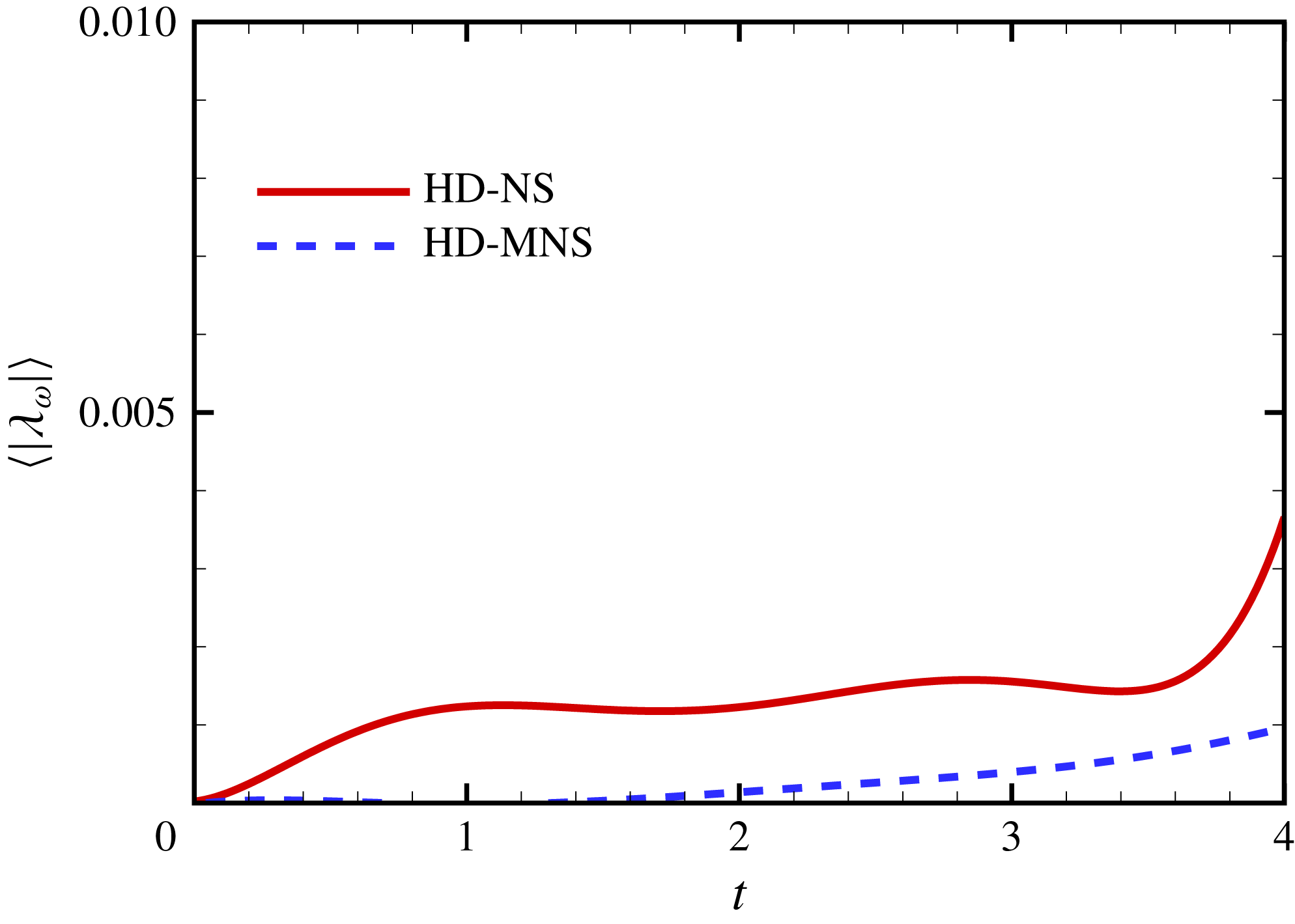
The averaged VSF deviations in two VSF calculations with different $\boldsymbol{V}$ in (4.7) in HD-NS and HD-MNS (see table 1) are compared in figure 4. Both $\langle |\unicode[STIX]{x1D706}_{\unicode[STIX]{x1D714}}|\rangle$ are very small (less than 1 %) at $t\leqslant 4$ in the temporal evolution of VSFs, and $\langle |\unicode[STIX]{x1D706}_{\unicode[STIX]{x1D714}}|\rangle$ in HD-MNS is even less than 0.1 % and is much smaller than that in HD-NS. For comparison, if we evolve $\unicode[STIX]{x1D719}_{v}$ as a passive scalar as (4.7) driven by physical velocity  $\boldsymbol{u}$ with the same initial VSF $\unicode[STIX]{x1D719}_{v0}$ , the VSF deviation at $t=4$ is relatively large as $\langle |\unicode[STIX]{x1D706}_{\unicode[STIX]{x1D714}}|\rangle \approx 10\,\%$ (Yang & Pullin Reference Yang and Pullin2010) owing to the breakdown of Helmholtz’s theorem (also see figure 2). These observations support the frozen-in nature of the VSF in the virtual velocity of the modified fluid flow, so we can accurately track vortex surfaces in some non-ideal flows. We remark that the singular virtual velocity at vorticity nulls has been smoothed in the numerical implementation described in § 4.1, so the modified fluid flow in case HD-MNS has a globally smooth virtual velocity everywhere.

Figure 4.

Temporal evolution of the volume-averaged VSF deviation in cases HD-NS and HD-MNS.

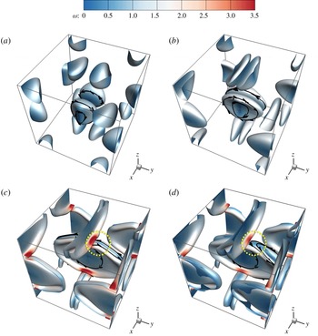
Moreover, the evolutions of VSF isosurfaces of $\hat{\unicode[STIX]{x1D719}}_{v}=0.5$ in HD-NS and HD-MNS are shown in figure 5, where the normalized VSF $\hat{\unicode[STIX]{x1D719}}_{v}$ for further improving the time coherence in VSF visualization (see Peng & Yang Reference Peng and Yang2018) is implicitly determined via $\hat{M}(\hat{\unicode[STIX]{x1D719}}_{v}=\unicode[STIX]{x1D711},t)=\hat{M}(\unicode[STIX]{x1D719}_{v0}=\unicode[STIX]{x1D711},t=0)$ . This normalization is performed by searching the isocontour values $\hat{\unicode[STIX]{x1D719}}_{v}=\unicode[STIX]{x1D711}$ at a given time $t$ and $\unicode[STIX]{x1D719}_{v0}$ at $t=0$ which correspond to the same fluid mass  $\hat{M}$ . The solid lines are vortex lines integrated from points on the surfaces, and they are attached on the VSF isosurfaces. This observation also indicates very small deviations in both VSF calculations.

Figure 5.

Temporal evolution of the VSF isosurface of $\hat{\unicode[STIX]{x1D719}}_{v}=0.5$ in case HD-NS or HD-MNS at $Re=100$ . Some vortex lines are integrated and plotted on the isosurfaces colour-coded by  $\unicode[STIX]{x1D714}$ . (a) HD-MNS, $t=1$ , (b) HD-MNS, $t=2$ , (c) HD-MNS, $t=4$ , (d) HD-NS, $t=4$ . The topological difference of the vortex lines in real TG flow (HD-NS) and modified TG flow (HD-MNS) is highlighted in yellow dotted circles in (c,d).

5.2 Reconnection of vortex lines

The geometry and topology in the evolution of vortex surfaces are important for characterizing flow transition in general and vortex reconnection (Kida & Takaoka Reference Kida and Takaoka1994) in particular. The vortex reconnection in the transition in both incompressible and compressible TG flows at a range of $Re$ has been extensively investigated in Yang & Pullin (Reference Yang and Pullin2011) and Peng & Yang (Reference Peng and Yang2018). The typical initial VSF isosurfaces with (4.6) are a pair of ellipsoid-like blobs. As shown in figure 5, the vortex surfaces are extracted as the VSF isosurface $\hat{\unicode[STIX]{x1D719}}=0.5$ colour-coded by $0\leqslant \unicode[STIX]{x1D714}\leqslant 3.5$ from blue to red. The vortex pair approach each other and are flattened in the evolution, and then they merge together with significant vorticity amplification at surface edges, signalling incipient vortex reconnection.

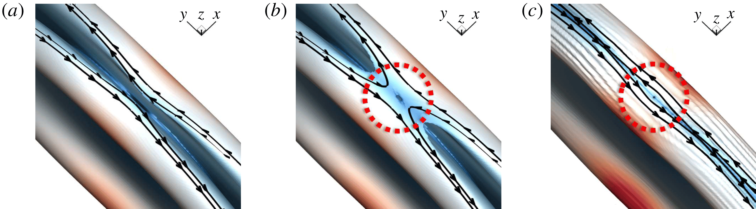
Before the vortex reconnection, the geometry of vortex surfaces and the topology of vortex lines in cases HD-NS and HD-MNS are very similar, so the VSF isosurfaces in HD-NS are not shown. During the vortex reconnection, the topology of vortex lines in HD-NS and HD-MNS is very different, as highlighted in the yellow dotted circle in figure 5(c,d). To further investigate the detailed process of the vortex reconnection, we zoom in on the VSF isosurfaces of $\hat{\unicode[STIX]{x1D719}}_{v}=0.5$ around their incipient reconnection time $t\approx 3.65$ in figure 6. The vortex reconnection is expected to occur on the symmetric planes of the periodic cube in case HD-NS, e.g. the vortex lines reconnect with the opposite vortex lines at the $y$ – $z$ plane at $x=\unicode[STIX]{x03C0}$ . We observe that the topology of vortex lines changes in the vicinity of the vorticity null highlighted in the red dotted circle in figure 6(b). In contrast, the topology of vortex lines in HD-MNS near $t=3.65$ , e.g. from $t=3.6$ to $t=3.7$ (not shown), is invariant in figure 6(c), and the vortex lines with opposite directions along the $y$ – $z$ plane at $x=\unicode[STIX]{x03C0}$ are almost parallel to each other. Thus the reconnection of vortex lines does not occur in the modified fluid flow. We remark that the approaching VSF isosurfaces appear to merge, but theoretically in between there should be a decreasing gap, which is not resolved under the present VSF grid resolution.

Figure 6.

Close-up view of the VSF isosurface of $\hat{\unicode[STIX]{x1D719}}_{v}=0.5$ near the vorticity null and the incipient reconnection time. Some vortex lines are integrated and plotted on the isosurfaces colour-coded by $0\leqslant \unicode[STIX]{x1D714}\leqslant 3.5$ . (a) HD-NS, $t=3.6$ , (b) HD-NS, $t=3.65$ , (c) HD-MNS, $t=3.65$ . The topological difference of the vortex lines in real TG flow (HD-NS) and modified TG flow (HD-MNS) is highlighted in red dotted circles in (b,c).

Based on the VSF evolution, we quantify the incipient vortex reconnection using the vorticity flux through the symmetric plane between a pair of approaching vortex surfaces (see Peng & Yang Reference Peng and Yang2018). Without loss of generality, we consider the vorticity flux through the $x$ – $z$ symmetric plane at $y=\unicode[STIX]{x03C0}$ between a pair of merging VSF isosurfaces of $\hat{\unicode[STIX]{x1D719}}_{v}=0.5$ . During the vortex reconnection, vortex lines are cut in the $y$ -direction and reconnected in the $x$ -direction. The vorticity fluxes through the $x$ – $z$ plane at $y=\unicode[STIX]{x03C0}$ and through the $y$ – $z$ plane at $x=\unicode[STIX]{x03C0}$ are defined as $\unicode[STIX]{x1D6F7}_{y}\equiv \int _{{\mathcal{S}}_{y}}\unicode[STIX]{x1D714}_{y}\,\text{d}{\mathcal{S}}$ and $\unicode[STIX]{x1D6F7}_{x}\equiv \int _{{\mathcal{S}}_{x}}\unicode[STIX]{x1D714}_{x}\,\text{d}{\mathcal{S}}$ , respectively. 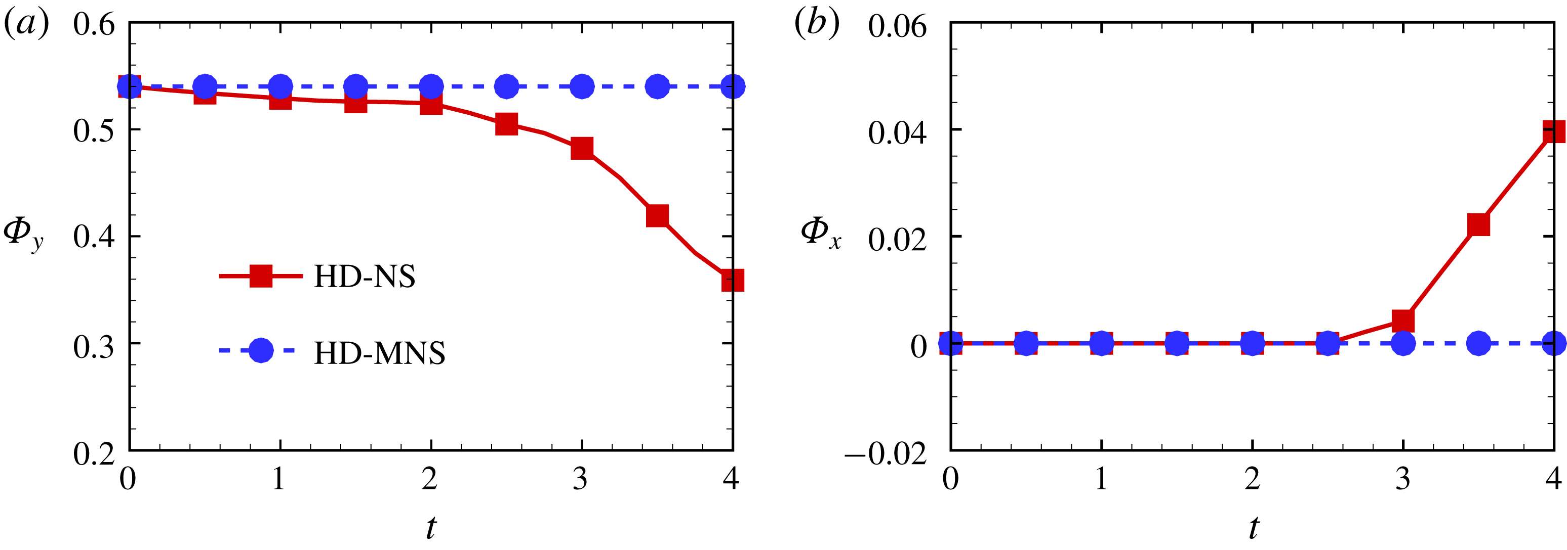Here, ${\mathcal{S}}_{y}$ and ${\mathcal{S}}_{x}$ are the regions enclosed by a half of the VSF contour line $\hat{\unicode[STIX]{x1D719}}_{v}=0.5$ and the $x$ – $y$ plane at $z=\unicode[STIX]{x03C0}$ on their corresponding symmetric planes. The temporal evolution of the vorticity fluxes in figure 7 shows that $\unicode[STIX]{x1D6F7}_{y}$ decreases and $\unicode[STIX]{x1D6F7}_{x}$ increases significantly around $t=2.6$ in case HD-NS, which indicates that the reconnection of vortex lines occurs as the exchange of vorticity directions through symmetric planes. In contrast, $\unicode[STIX]{x1D6F7}_{x}$ and $\unicode[STIX]{x1D6F7}_{y}$ in HD-MNS are conserved during the evolution.

This quantification implies that the reconnection of vortex lines is prohibited in the modified fluid flow in HD-MNS. In other words, the vortex lines in a non-ideal, dissipative flow can still have topological invariance. This result agrees with (2.12) for the virtual conservation of vorticity flux, (2.19) for the virtual conservation of helicity and the visualization of vortex lines in figures 5 and 6. In the framework of the virtual velocity, the reconnection of vortex lines is triggered by non-vanishing $\boldsymbol{F}_{\Vert }$ in NS equations or vorticity nulls.

Figure 7.

Temporal evolution of the vorticity fluxes through symmetric planes. (a)  $\unicode[STIX]{x1D6F7}_{y}$ and (b)  $\unicode[STIX]{x1D6F7}_{x}$ .

6.1 Spurious deformation of vortex surfaces

In MHD TG flows, the non-ideal force term $\boldsymbol{F}=\boldsymbol{F}_{\unicode[STIX]{x1D708}}+\boldsymbol{F}_{L}$ in MHD equations (4.3) includes the viscous term $\boldsymbol{F}_{\unicode[STIX]{x1D708}}=\unicode[STIX]{x1D708}\unicode[STIX]{x1D6FB}^{2}\boldsymbol{u}$ and the Lorentz force term $\boldsymbol{F}_{L}=\boldsymbol{j}\times \boldsymbol{b}$ . As discussed in § 5 and Yang & Pullin (Reference Yang and Pullin2010), the viscous effect in HD TG flows is negligible on vortex evolution with high $Re$ until significant vortex reconnection. By contrast, the non-ideal effect in MHD TG flows, dominated by the Lorentz force term, can have an impact on tracking vortex surfaces.

For case MHD-S, the vorticity in the reduced MHD equations (4.4) has an exact solution

(6.1) $$\begin{eqnarray}\unicode[STIX]{x1D74E}(\boldsymbol{x},t)=\unicode[STIX]{x1D74E}_{0}\text{e}^{-\unicode[STIX]{x1D708}t},\end{eqnarray}$$

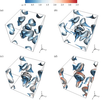
where $\unicode[STIX]{x1D74E}_{0}$ denotes the initial vorticity. This solution indicates that the geometry and topology of vortex lines are invariant in MHD-S. Nonetheless, if the VSF is calculated as (3.3) driven by the physical velocity $\boldsymbol{u}$ using the two-time method in MHD-S, which is similar to dye visualization in experiments, we find that the evolving VSF isosurface has significant geometrical and topological changes. In figure 8, VSF isosurfaces evolve from initial ellipsoids, and then they appear to collide and merge with significant deformation. This observation contradicts the steady vortex lines implied in (6.1).

Figure 8.

The spurious deformation of vortex surfaces in non-ideal flows is illustrated by the evolving VSF isosurface of $\hat{\unicode[STIX]{x1D719}}_{v}=0.5$ in case MHD-S at $Re=100$ . Some vortex lines are integrated and plotted on the isosurfaces colour-coded by  $\unicode[STIX]{x1D714}$ . (a)  $t=0$ , (b)  $t=1$ , (c)  $t=2$ , (d)  $t=3$ .

This inconsistency implies that convecting VSF along the physical velocity in MHD flows with strong non-ideal forces can result in spurious deformation of vortex surfaces. Moreover, the VSF solution in MHD-S is still accurate with $\langle |\unicode[STIX]{x1D706}_{\unicode[STIX]{x1D714}}|\rangle <1\,\%$ as the perfect attachment of vortex lines in figure 8. Although the deviation of VSF solutions owing to non-ideal forces is corrected in the two-time method, one VSF solution can evolve into another VSF solution.

The spurious deformation of VSF isosurfaces manifests the non-uniqueness of VSF solutions, but it can be eliminated by convecting the VSF along the virtual velocity as in case MHD-SV. For the steady MHD TG flow with $\unicode[STIX]{x1D708}=\unicode[STIX]{x1D702}=0$ , the drift velocity has the exact solution $\boldsymbol{v}_{d}=-\boldsymbol{u}$ , then the virtual VSF transport (3.5) with the vanishing virtual velocity $\boldsymbol{v}=0$ is reduced to the steady VSF equation $\unicode[STIX]{x2202}\unicode[STIX]{x1D719}_{v}/\unicode[STIX]{x2202}t=0$ . In other words, the motion driven by the drift velocity cancels the spurious deformation induced by non-ideal forces, so that we can obtain the vortex surfaces with invariant geometry and topology in MHD-SV, which agrees with the theoretical solution (6.1).

6.2 Tracking vortex surfaces in the approximate virtual velocity

As discussed in § 4.4, when the explicit virtual velocity does not exist, we can still seek a good approximate virtual velocity in the non-ideal flows in which $\boldsymbol{F}$ has a preferential normal alignment with  $\unicode[STIX]{x1D74E}$ . 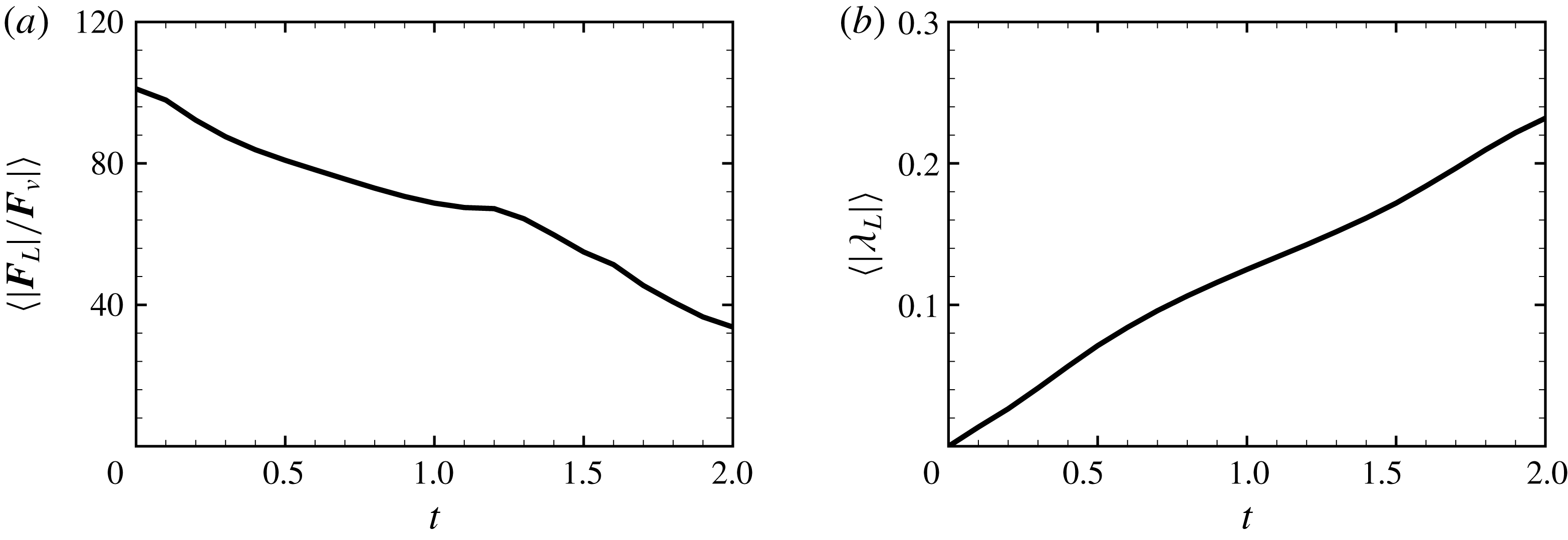For the insulating MHD TG flow in case MHD-I, both $\boldsymbol{F}_{\unicode[STIX]{x1D708}}$ and $\boldsymbol{F}_{L}$ are perpendicular to $\unicode[STIX]{x1D74E}$ at the initial time. On average, $|\boldsymbol{F}_{L}|$ is at least an order of magnitude greater than $|\boldsymbol{F}_{\unicode[STIX]{x1D708}}|$ at $0\leqslant t\leqslant 2$ in figure 9(a), so the Lorentz force dominates the non-ideal force and then we neglect the viscous effect in $\boldsymbol{F}$ during the time interval of interest.

The preferential normal alignment between $\boldsymbol{F}_{L}$ and $\unicode[STIX]{x1D74E}$ is quantified by the volume average of

(6.2) $$\begin{eqnarray}\unicode[STIX]{x1D706}_{L}\equiv {\displaystyle \frac{\boldsymbol{F}_{L}\boldsymbol{\cdot }\unicode[STIX]{x1D74E}}{|\boldsymbol{F}_{L}|\,|\unicode[STIX]{x1D74E}|}}.\end{eqnarray}$$

The growing $\langle |\unicode[STIX]{x1D706}_{L}|\rangle$ in figure 9(b) implies that the preferential normal alignment is suppressed with time, but $\langle |\unicode[STIX]{x1D706}_{L}|\rangle <0.25$ still maintains at a relatively small value. Thus we consider the approximate virtual velocity (2.37) as

(6.3) $$\begin{eqnarray}\boldsymbol{v}=\boldsymbol{u}+\frac{\unicode[STIX]{x1D74E}\times \boldsymbol{F}_{L}}{\unicode[STIX]{x1D714}^{2}},\end{eqnarray}$$

and we will demonstrate that this approximate virtual velocity can effectively reduce the spurious deformation of vortex surfaces discussed in § 6.1 to improve the vorticity flux conservation in the virtual evolution.

Figure 9.

Temporal evolution of volume-averaged quantities in the insulating MHD TG flow at $Re=100$ . (a) Ratio of the magnitudes of Lorentz force term to viscous term. (b) Preferential normal alignment between $\boldsymbol{F}_{L}$ and  $\unicode[STIX]{x1D74E}$ .

Temporal evolutions of VSF isosurfaces $\unicode[STIX]{x1D719}_{v}=0.5$ in cases MHD-I and MHD-IV at $Re=100$ are shown in figures 10 and 11, respectively. The VSF deviation $\langle |\unicode[STIX]{x1D706}_{\unicode[STIX]{x1D714}}|\rangle <1\,\%$ is very small for both cases at $0\leqslant t\leqslant 2$ , and vortex lines almost lie on the VSF isosurfaces. We observe that the evolutions of vortex surfaces in the two cases display significant differences in both evolutionary topology and geometry.

Figure 10.

Temporal evolution of the VSF isosurface of $\hat{\unicode[STIX]{x1D719}}_{v}=0.5$ in case MHD-I at $Re=100$ , where the VSF is convected by the physical velocity. Some vortex lines are integrated and plotted on the isosurfaces colour-coded by $\unicode[STIX]{x1D714}$ . (a)  $t=0.5$ , (b)  $t=1.0$ , (c)  $t=1.5$ , (d)  $t=2.0$ .

Figure 11.

Temporal evolution of the VSF isosurface of $\hat{\unicode[STIX]{x1D719}}_{v}=0.5$ in case MHD-IV at $Re=100$ , where the VSF is convected by the virtual velocity. Some vortex lines are integrated and plotted on the isosurfaces colour-coded by $\unicode[STIX]{x1D714}$ . (a)  $t=0.5$ , (b)  $t=1.0$ , (c)  $t=1.5$ , (d)  $t=2.0$ .

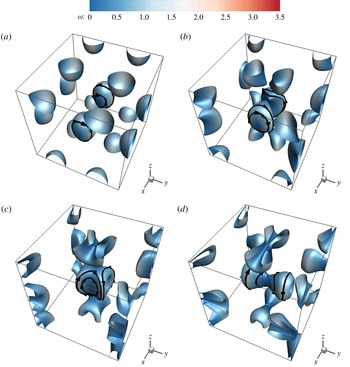
In MHD-I, the VSF is primarily convected by the physical velocity $\boldsymbol{u}$ in the two-time method. Comparing with the VSF evolution in HD TG flows in figure 5, we observe in figure 10 that long tubular structures are stretched out from the approaching vortex surfaces at $t=1$ under the influence of strong non-ideal Lorentz force. Then these structures are shortened at $t=1.5$ and $t=2$ . Furthermore, the two approaching vortex surfaces do not merge at $t=2$ .

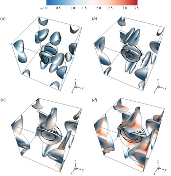
In MHD-IV, the VSF is convected by the approximate virtual velocity (6.3). The evolution of vortex surfaces in figure 11 is similar to that in HD TG flows in figure 5. The approaching surfaces are only flattened at $0\leqslant t\leqslant 1$ without the small-scale protruding structures in figure 10(b). As discussed in § 6.1, the protruding structures appear to be spurious deformation owing to the non-uniqueness of VSF solutions. In figure 11(b), they are eliminated by incorporating the virtual velocity in the tracking of vortex surfaces. After $t=1$ , the two vortex surfaces merge together and the reconnection of vortex lines occurs around $t=1.5$ .

6.3 Virtual conservation of vorticity flux

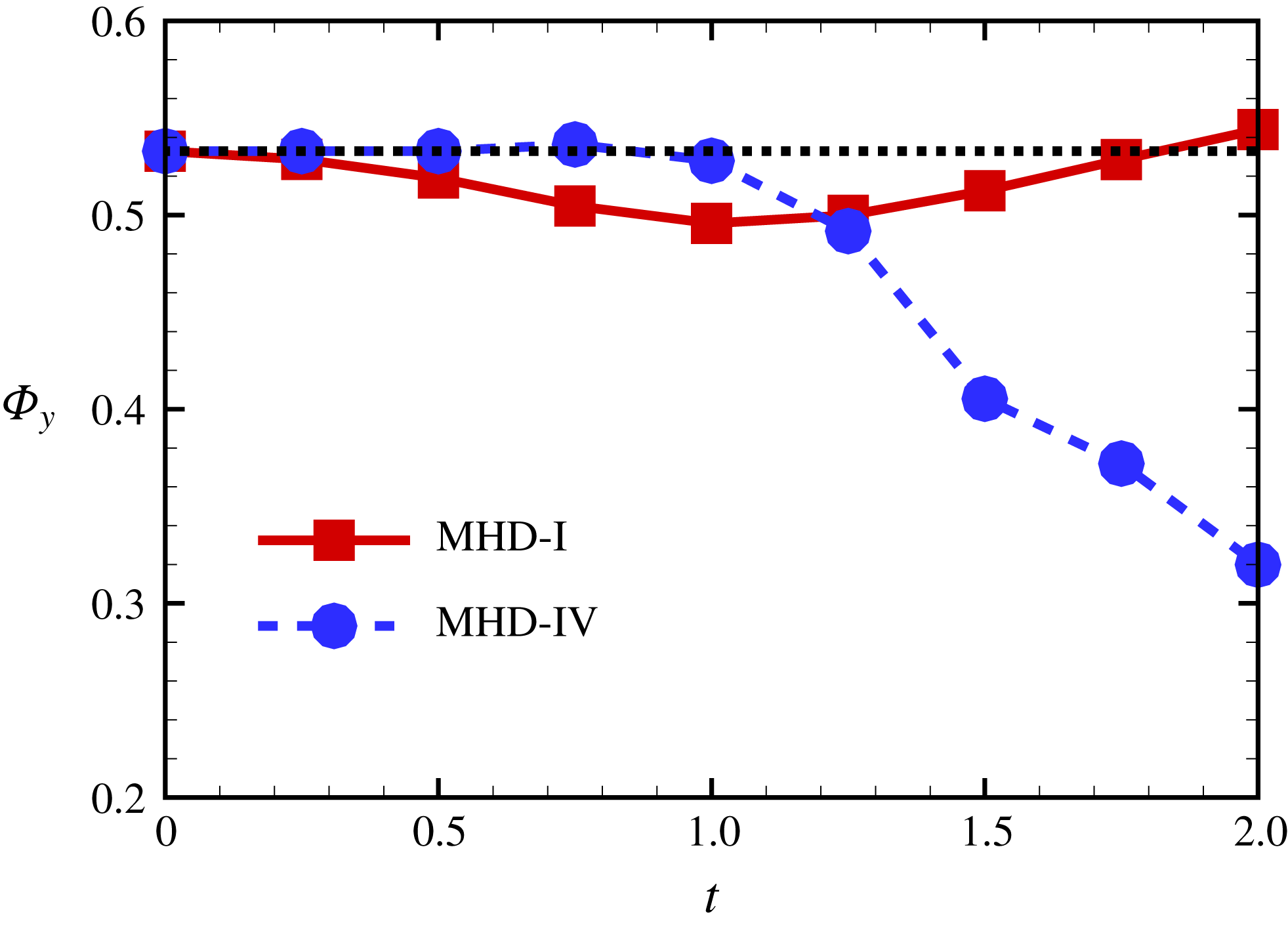
Virtual Helmholtz’s theorem (2.12) suggests that the vorticity flux is conserved in tracking vortex surfaces along a smooth virtual velocity (also see figure 2). Without loss of generality, the evolution of vorticity flux $\unicode[STIX]{x1D6F7}_{y}$ through the $x$ – $z$ symmetric plane at $y=\unicode[STIX]{x03C0}$ is shown in figure 12. In MHD-IV, $\unicode[STIX]{x1D6F7}_{y}$ is almost conserved before $t=1$ as the VSF isosurfaces have not touched the vorticity nulls at the centre in figure 11(b). After $t=1$ , the rapid decay of $\unicode[STIX]{x1D6F7}_{y}$ signals the incipient reconnection of vortex lines in figure 11(c). This trend is consistent with the decaying of $\unicode[STIX]{x1D6F7}_{y}$ in HD TG flows in figure 7(a). By contrast, $\unicode[STIX]{x1D6F7}_{y}$ in MHD-I is not conserved throughout the entire evolution.

Figure 12.

Temporal evolution of vorticity flux $\unicode[STIX]{x1D6F7}_{y}$ through the $x$ – $z$ symmetric plane at $y=\unicode[STIX]{x03C0}$ . The dotted line denotes the value of $\unicode[STIX]{x1D6F7}_{y}$ at $t=0$ .

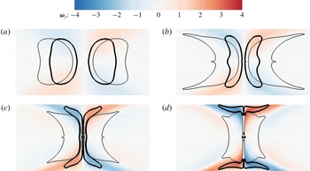
Figure 13 displays the boundaries of VSF isosurfaces in MHD-I (grey thin lines) and MHD-IV (black thick lines) on the $x$ – $z$ symmetric plane at $y=\unicode[STIX]{x03C0}$ . At $t=0$ , the approaching motion of the vortex pair driven by the virtual velocity $\boldsymbol{v}\approx 2\boldsymbol{u}$ is much faster than that driven by  $\boldsymbol{u}$ . Then the vortex pair in MHD-IV is also flattened and merged more quickly than that in MHD-I. We observe that the VSF contour lines in MHD-IV can capture the regions with significant vorticity intensification, whereas the contour lines in MHD-IV do not well coincide with the regions with growing  $\unicode[STIX]{x1D6F7}_{y}$ . This observation supports that better conservation of $\unicode[STIX]{x1D6F7}_{y}$ is achieved in MHD-IV than in MHD-I before the merging of vortex surfaces.

Figure 13.

Comparison of the VSF evolutions convected by the physical velocity in case MHD-I and convected by the virtual velocity in case MHD-IV on the $x$ – $z$ symmetric plane within $0\leqslant x\leqslant 2\unicode[STIX]{x03C0}$ and $\unicode[STIX]{x03C0}/2\leqslant z\leqslant 3\unicode[STIX]{x03C0}/2$ at $y=\unicode[STIX]{x03C0}$ . Thick black and thin grey lines are contour lines of $\hat{\unicode[STIX]{x1D719}}_{v}=0.5$ in MHD-IV and MHD-I, respectively. The contour is colour-coded by $\unicode[STIX]{x1D714}_{y}$ . (a)  $t=0.5$ , (b)  $t=1.0$ , (c)  $t=1.5$ , (d)  $t=2.0$ .

The similarities on the evolutionary geometry of vortex surfaces in figures 5 and 10 indicate that the vortex dynamics in HD TG flow and insulating MHD TG flow appears to be essentially the same before the vortex reconnection, but the incipient reconnection of vortex surfaces with larger $\boldsymbol{v}_{d}$ in MHD-IV occurs earlier than that in HD-NS. Since vortex lines are stretched during the vortex reconnection (see Yang & Pullin Reference Yang and Pullin2011), the total energy or enstrophy in the insulating MHD TG flow is smaller or larger than that in the HD TG flow in figure 3. Therefore, the time for the turbulent transition at larger $Re$ or the potential finite-time singularity in the inviscid limit in MHD TG flows (see Lee et al. Reference Lee, Brachet, Pouquet, Rosenberg and Mininni2009) is earlier than that in corresponding HD flows (see Brachet et al. Reference Brachet, Meiron, Orszag, Nickel, Morf and Frisch1983).

In addition, the boundaries of VSF isosurfaces in MHD-I (grey thin lines) and MHD-IV (black thick lines) on the $x$ – $y$ symmetric plane at $z=\unicode[STIX]{x03C0}$ are shown in figure 14. The acceleration of vortex motion in the virtual Lagrangian view is depicted by the contour of the $x$ -component of $\boldsymbol{v}_{d}$ . The outward spiral streamlines of the virtual velocity sweep vortex surfaces towards impermeable planes faster than the closed streamlines (not shown) of the physical velocity.

Figure 14.

Comparison of the VSF evolutions convected by the physical velocity in case MHD-I and convected by the virtual velocity in case MHD-IV with streamlines of the virtual velocity on the $x$ – $y$ symmetric plane within $0\leqslant x\leqslant \unicode[STIX]{x03C0}$ and $0\leqslant y\leqslant \unicode[STIX]{x03C0}$ at $z=\unicode[STIX]{x03C0}$ . Thick black and thin grey lines are contour lines of $\hat{\unicode[STIX]{x1D719}}_{v}=0.5$ in MHD-IV and MHD-I, respectively. The contour is colour-coded by $-1.3\leqslant v_{d,x}\leqslant 1.3$ from blue to red. (a)  $t=0.5$ , (b)  $t=1.5$ .

In non-ideal flows, the results in this section demonstrate that tracking vortex surfaces in the virtual velocity appears to be more physically reasonable than tracking in the physical velocity. First, tracking vortex surfaces in the physical velocity can cause spurious deformation in flows with strong non-ideal forces, whereas tracking in the virtual velocity can eliminate such an artifact. Second, tracking in the virtual velocity has better conservation of vorticity flux and other vorticity-related quantities than tracking in the physical velocity.