INTRODUCTION
In the early 1950s Hans Suess described a significant decrease in the radiocarbon content of the atmosphere due to the combustion of fossil fuels, which contain virtually no radiocarbon and therefore dilute atmospheric 14C relative to 12C (Suess Reference Suess1953, Reference Suess1955). This trend changed dramatically in the late 1950s and early 1960s when nuclear-bomb tests increased atmospheric radiocarbon content to levels not ever seen before in the last 50,000 years of Earth’s history. Since then, radiocarbon content has been declining globally as evidenced by data from tree-rings and more recent direct atmospheric observations (Tans et al. Reference Tans, de Jong and Mook1979; Manning et al. Reference Manning, Lowe, Melhuish, Sparks, Wallace, Brenninkmeijer and McGill1990; Levin et al. Reference Levin, Schuchard, Kromer and Muennich1989; Currie et al. Reference Currie, Brailsford, Nichol, Gomez, Sparks, Lassey and Riedel2011; Graven et al. Reference Graven, Guilderson and Keeling2012; Hua et al. Reference Hua, Barbetti and Rakowski2013; Levin et al. Reference Levin, Kromer and Hammer2013).
Using a simple box model of the global carbon cycle, Caldeira et al. (Reference Caldeira, Rau and Duffy1998) predicted that atmospheric radiocarbon content will continue a negative rate of decline until the beginning of the 21st century and will return to pre-1950 values around the year 2020. More recently, Graven (Reference Graven2015) predicted a similar time for returning to pre-1950s values, but with different trajectories according to different fossil-fuel emission scenarios. This point, where Δ14C values go from positive to negative, indicate a transition where fossil-fuel derived CO2 dominates the atmospheric signal of radiocarbon, previously dominated by bomb-derived radiocarbon.
Determining this transition point in atmospheric radiocarbon is important for different reasons. For instance, a) it helps to determine the impact of fossil fuel emissions on the global carbon cycle (Caldeira et al. Reference Caldeira, Rau and Duffy1998; Turnbull et al. Reference Turnbull, Rayner, Miller, Naegler, Ciais and Cozic2009; Graven Reference Graven2015), b) it serves as an important benchmark for global carbon models since the rate of radiocarbon decline is the result of different processes rates in global C reservoirs, and appropriate representation of these processes in models must predict accurately this transition point (Oeschger et al. Reference Oeschger, Siegenthaler, Schotterer and Gugelmann1975; Randerson et al. Reference Randerson, Enting, Schuur, Caldeira and Fung2002; Naegler and Levin Reference Naegler and Levin2006), and c) it sets a new reference point for dating organic material of interest in biology, biogeochemistry, forensics and archeology (Graven Reference Graven2015).
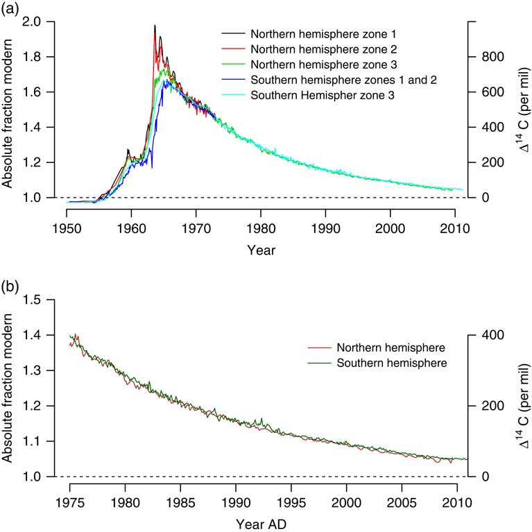
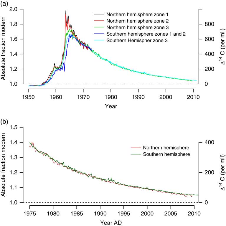
Post-bomb atmospheric radiocarbon data for different hemispheric zones have been compiled and homogenized by Hua et al. (Reference Hua, Barbetti and Rakowski2013), harmonizing measurements from tree-rings (e.g. Hertelendi and Csongor Reference Hertelendi and Csongor1983; Levin and Kromer Reference Levin and Kromer1997; Hua et al. Reference Hua, Barbetti, Jacobsen, Zoppi and Lawson2000; Park et al. Reference Park, Kim, Cheoun, Kim, Youn, Liu and Kim2002; Yamada et al. Reference Yamada, Yasuike and Komura2005; Hua et al. Reference Hua, Barbetti, Levchenko, D’Arrigo, Buckley and Smith2012; Rakowski et al. Reference Rakowski, Nadeau, Nakamura, Pazdur, Pawełczyk and Piotrowska2013) and direct atmospheric observations (e.g. Vogel and Marais Reference Vogel and Marais1971; Berger et al. Reference Berger, Jackson, Michael and Suess1987; Manning et al. Reference Manning, Lowe, Melhuish, Sparks, Wallace, Brenninkmeijer and McGill1990; Nydal and Loevseth Reference Nydal and Loevseth1996; Levin and Kromer Reference Levin and Kromer2004; Meijer et al. Reference Meijer, Pertuisot and van der Plicht2006; Turnbull et al. Reference Turnbull, Lehman, Miller, Sparks, Southon and Tans2007; Levin et al. Reference Levin, Naegler, Kromer, Diehl, Francey, Gomez-Pelaez, Steele, Wagenbach, Weller and Worthy2010; Currie et al. Reference Currie, Brailsford, Nichol, Gomez, Sparks, Lassey and Riedel2011; Graven et al. Reference Graven, Guilderson and Keeling2012) (Figure 1). These hemispheric “bomb curves” contain very useful information on the trend and seasonality of atmospheric radiocarbon for different hemispheric regions. Furthermore, this information can be used to forecast future trends in atmospheric radiocarbon and determine the possible transition date to pre-1950 levels.
Atmospheric radiocarbon curves obtained by Hua et al. (Reference Hua, Barbetti and Rakowski2013). (a) Original data for four different atmospheric regions, (b) time series constructed from original data for the period 1975 to 2010. (See online version for color figures.)
Compiled atmospheric radiocarbon curves are only released to the scientific community at irregular intervals (Hua and Barbetti Reference Hua and Barbetti2004; Hua et al. Reference Hua, Barbetti and Rakowski2013), and there is a need to produce forecasts of these curves for periods not covered by the compiled curves. For instance, radiocarbon dating methods or analyses of cycling rates in carbon reservoirs using samples from recently collected material require best estimates of the atmospheric radiocarbon values for time intervals after the latests release of the compiled radiocarbon curves (Sierra et al. Reference Sierra, Müller and Trumbore2014). For this reason, it is important to provide robust statistical methods for forecasting that can provide accurate predictions.
Here I present a time-series decomposition analysis for the atmospheric radiocarbon curves of Hua et al. (Reference Hua, Barbetti and Rakowski2013), fitting a set of exponential smoothing state-space models with the aim to forecast future trends in radiocarbon at hemispheric scales. The main objectives of this analysis are, a) to decompose the observed time series into trend and seasonal components and characterize differences among hemispheric zones, and b) to identify the probability of returning to pre-bomb radiocarbon values; i.e. Δ14C≤0‰. Additionally, I present radiocarbon measurements of plants from different cities to identify the degree at which, by local dilution, atmospheric radiocarbon has already crossed this threshold.
METHODS
Time Series Decomposition
I used the harmonized atmospheric radiocarbon time series reported by Hua et al. (Reference Hua, Barbetti and Rakowski2013) for the northern and southern hemispheres. Although these authors present curves for five different hemispheric zones, the curves only deviate from each other during the early bomb period. Here, I used data from the years 1975 to 2010, where intra-hemispheric differences are not reported, and only the northern and the southern hemispheres are differentiated.
These hemispheric radiocarbon time-series are not available at regularly spaced intervals as required by the time-series analysis used here; therefore, they were homogenized in regular monthly and seasonal periods by cubic spline interpolation (Figure 1b).
To analyze each time series, I used the ETS framework described by Hyndman et al. (Reference Hyndman, Koehler, Ord and Snyder2008) to fit 30 different exponential smoothing state-space models that decompose the series in the error (E), trend (T), and seasonal (S) components (ETS decomposition). In classical time-series decomposition methods, trend, seasonality and error are commonly assumed as linear additive terms (e.g. Cleveland et al. Reference Cleveland, Freeny and Graedel1983), which in the ETS framework imply a model of the form E+T+S. However, many other methods have been proposed to decompose time series in its inherent components, not only considering linear additive models. For instance, models can have all terms multiplicative (E*T*S), or combinations between additive and multiplicative terms (e.g. E*T+S). The different combinations of potential model structures results in the 30 different models tested here. As selection criterion, I used the Akaike information criterion (AIC), which selects the best model according to goodness of fit and the complexity of the model, given preference to the simplest model that can best predict the observations.
When the data contains zeros or negative values, the multiplicative error models in the ETS framework are not numerically stable (Hyndman et al. Reference Hyndman, Koehler, Ord and Snyder2008). For this reason, I used the radiocarbon series as absolute fraction modern F′ in all computations (Trumbore et al. Reference Trumbore, Sierra and Hicks Pries2016), which expresses Δ14C values as a fraction by the relation
 $$\Delta ^{{14}} {\rm C}{\,\equals\,}\left( {F{{\rm \prime}} {\,\minus\,}1} \right) \cdot 1000,{\rm }$$
and can also be interpreted as fraction modern F corrected for radioactive decay of the OX1 standard since 1950. More precisely,
 $$F{\rm '}{\,\equals\,}F \cdot {\rm exp}((1950{\,\minus\,}x)/8267),$$
where x is the year of sample collection.
ETS models predict observations y t according to a function of the error, trend, and seasonal components f(E,T,S). The trend component is also split between a level l and a growth term b. The error term ε is considered a Gaussian white-noise process with variance σ 2. The mean value of the observations is therefore predicted by a function
 $$\mu _{t} {\,\equals\,}f(l,b,s,\theta ),$$
where s is the seasonal trend and θ are a set of constant parameters that weigh the contributions from the different components. Parameter estimation is performed by maximum likelihood.
Forecasting is performed by recursively applying the ETS model h number of steps ahead the last observation. Specific details about the method and its implementation in the R package forecast are provided in Hyndman et al. (Reference Hyndman, Koehler, Ord and Snyder2008) and Hyndman and Khandakar (Reference Hyndman and Khandakar2008), respectively. In the supplementary material I provide all code necessary to reproduce the results presented here.
Radiocarbon in Local Air
I also used radiocarbon analyses of annual plants to infer the atmospheric radiocarbon concentration in a set of cities around the world. Annual plants incorporate local sources of carbon dioxide during the growing season, providing an integrated measure of the radiocarbon concentration of the local air (Hsueh et al. Reference Hsueh, Krakauer, Randerson, Xu, Trumbore and Southon2007). For consistency, I sampled at each location at least three individuals of dandelion (Taraxacum spp.), an annual plant that can be found growing in most cities. For comparison, I also sampled plants at locations with low influence of anthropogenic fossil fuel emissions such as the Rocky Mountain National Park (RMNP) in the USA, the Austrian Alps, and in the Amazon basin at the town of Leticia, Colombia. Plants were washed and air-dried after sampling to eliminate contamination from dust and other particles. All samples were then oven-dried at 70° Celsius and ground in a ball-grinder at the Max Planck Institute for Biogeochemistry in Jena, Germany. Radiocarbon analyses were conducted by Accelerator Mass Spectrometry at the same institution (Steinhof et al. Reference Steinhof, Adamiec, Gleixner, Wagner and van Klinken2004).
RESULTS
Time Series Decomposition
From the 30 different competing models, the best performance was obtained by an ETS model of the form: (M,A,M), which means that the error and the seasonal terms are multiplicative, and the trend term is additive. Specifically, for both hemispheric curves the model with the best AIC had the form:
 $$\eqalignno{ & \mu _{t} {\,\equals\,}(l_{{t{\minus}1}} {\plus}b_{{t{\minus}1}} )s_{{t{\minus}m}} , \cr & l_{t} {\,\equals\,}(l_{{t{\minus}1}} {\plus}b_{{t{\minus}1}} )(1{\plus}\alpha {\varepsilon}_{t} ), \cr & b_{t} {\,\equals\,}b_{{t{\minus}1}} {\plus}\beta (l_{{t{\minus}1}} {\plus}b_{{t{\minus}1}} ){\varepsilon}_{t} , \cr & s_{t} {\,\equals\,}s_{{t{\minus}m}} (1{\plus}\gamma {\varepsilon}_{t} ),$$
where α, β, and γ are constant parameters, and the t−m subscript represents the intra-annual time-step that composes the seasonal cycle of the seasonal term s.
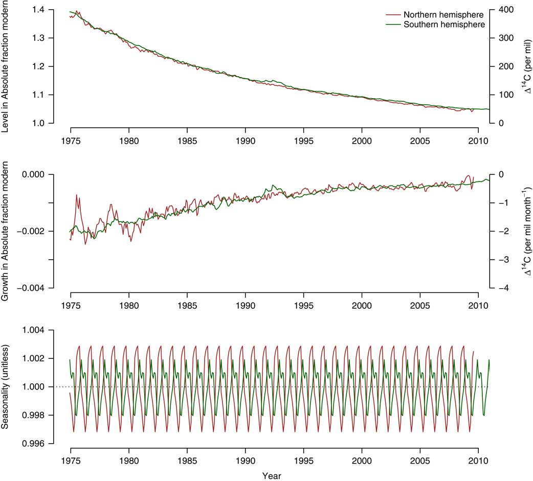
For the northern hemisphere time series, the value of the parameters were θ NH : (α=0.7551, β=0.0346, γ=0.0001); and for the southern hemisphere θ SH : (α=0.2504, β=0.0086, γ=0.0001). Notice that the main differences among the two models are on the parameters α and β that control the degree by which the error term influence the level and growth terms, respectively. This implies that for the northern hemisphere, the level and the growth terms showed more variability than in the southern hemispheres (Figure 2). The seasonal term had very little influence from the error term as predicted by γ, therefore the seasonal cycle obtained from this model had a very regular pattern.
Trend (level and slope) and seasonality of the atmospheric radiocarbon time series predicted by the best-fit model for the hemispheric series compiled by Hua et al. (Reference Hua, Barbetti and Rakowski2013). For both series, the best model selected based on the AIC was an ETS model of the form (M,A,M), i.e. a multiplicative term for the error, an additive term for the trend, and a multiplicative term for the seasonality.
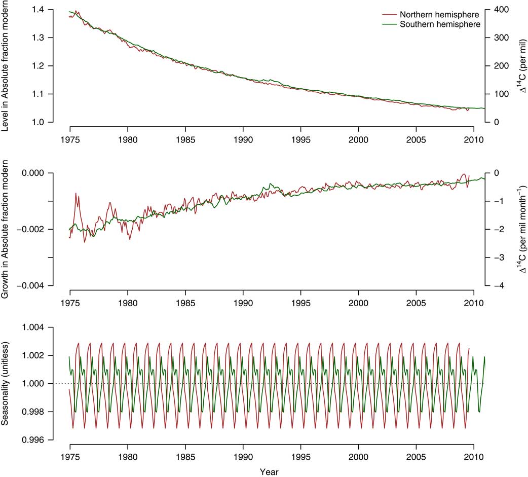
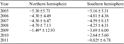
The temporal pattern of the growth term b t was relatively similar between the northern and the southern hemispheres (Figure 2b), but the curve for the level term was always lower for the northern hemisphere, which results in a larger decline of atmospheric radiocarbon for the north (Figure 2a). For the last years in both time series, from 2005 to 2011, the annual decline in atmospheric radiocarbon in Δ14C was below −5‰ in both hemispheres, but with relatively high uncertainty as accounted by the ε term (Table 1).
Slopes of the atmospheric radiocarbon curves (± residuals ε t ) calculated for the last years of the series using the obtained ETS model. Values in Δ14C (per mil/yr).

* Only includes the first 8 months of the year.
† Only includes the first 3 months of the year.
Since the seasonal pattern is a multiplicative term centered around 1, the absolute amplitude of the seasonal cycle is predicted to decline in this model for both hemispheres, but proportionally to the actual radiocarbon concentration in the atmosphere. The lower the value of the trend (l + b) the lower the amplitude of the term μ t . The model predicts a higher influence of the seasonal term for the northern than for the southern hemisphere. The model also predicts, as previously reported (Levin et al. Reference Levin, Naegler, Kromer, Diehl, Francey, Gomez-Pelaez, Steele, Wagenbach, Weller and Worthy2010; Currie et al. Reference Currie, Brailsford, Nichol, Gomez, Sparks, Lassey and Riedel2011), a reversed seasonality between the northern and the southern hemispheres (Figure 2c).
Forecast
A forecast of the atmospheric radiocarbon time series was obtained by exponential smoothing of the ETS model, i.e. recursively applying the set of equations with the best parameter values found (Hyndman et al. Reference Hyndman, Koehler, Ord and Snyder2008). The forecast was obtained on quarterly intervals and not on a monthly basis since the multiplicative error term strongly influences uncertainty bounds in predictions at short-time scales. This is a relatively well-known issue in forecasting methods (Athanasopoulos et al. Reference Athanasopoulos, Hyndman, Kourentzes and Petropoulos2017), and it is commonly recommended to produce forecasts at an intermediate time-scale such as every four months in long-term monthly time-series (Nijman and Palm Reference Nijman and Palm1990; Rossana and Seater Reference Rossana and Seater1995; Athanasopoulos et al. Reference Athanasopoulos, Hyndman, Kourentzes and Petropoulos2017).
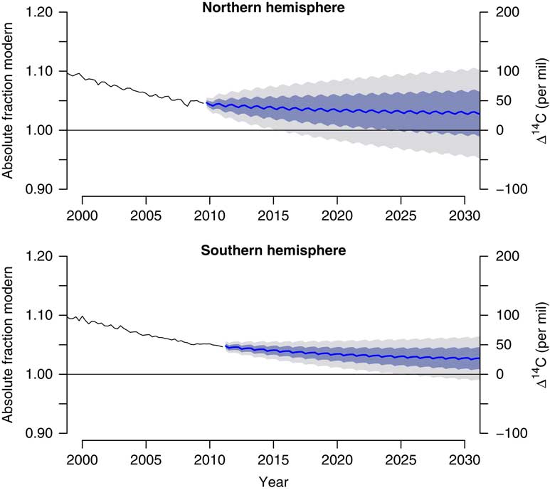
For the two series, the forecast of the average radiocarbon values showed a linear decrease for the next 20 years (Figure 3). This linear decline is based on the observed stabilization of the growth term of the time series (Figure 2a). The range of the prediction intervals increases in all series because of the nature of the exponential smoothing model that assigns less weight to successively older observations and therefore the uncertainty in the predictions increases.
Forecast of atmospheric radiocarbon for the northern and southern hemispheres based on the best ETS model. Shaded regions in gray and blue show the 95 and 68% prediction intervals.
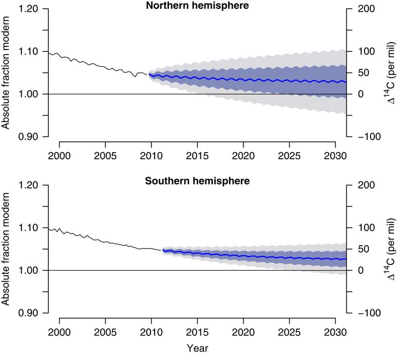
Atmospheric radiocarbon is predicted to decline faster in the northern hemisphere than in the southern hemisphere, therefore it is more likely that radiocarbon values return to pre-1950 values earlier in the northern hemisphere. Uncertainty ranges are also higher for the northern than for the southern hemisphere as a consequence of higher values of the parameters α and β from the ETS model.
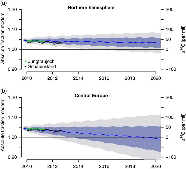
Independent observations of atmospheric radiocarbon from European stations at the Schauinsland and Jungfraujoch sites (Levin et al. Reference Levin, Kromer and Hammer2013), are within forecast uncertainty range for the northern hemisphere (Figure 4a). The observations from Jungfraujoch follow relatively well the forecasted mean and the seasonal cycle; however for Schauinsland, the independent observations are below the forecasted mean. One likely explanation for this difference in the Schauinsland station, is the potential contribution of fossil-fuel derived carbon from the nearby city of Freiburg, Germany (Levin et al. Reference Levin, Schuchard, Kromer and Muennich1989; Turnbull et al. Reference Turnbull, Rayner, Miller, Naegler, Ciais and Cozic2009; Levin et al. Reference Levin, Kromer and Hammer2013).
(a) Forecast (with 68 and 95% prediction intervals) for the northern hemisphere radiocarbon curve compared to observations at the Jungfraujoch and Schauinsland reported in Levin et al. (Reference Levin, Kromer and Hammer2013). (b) Optimized forecast for central Europe forcing the model to pass through the observations from these two stations.
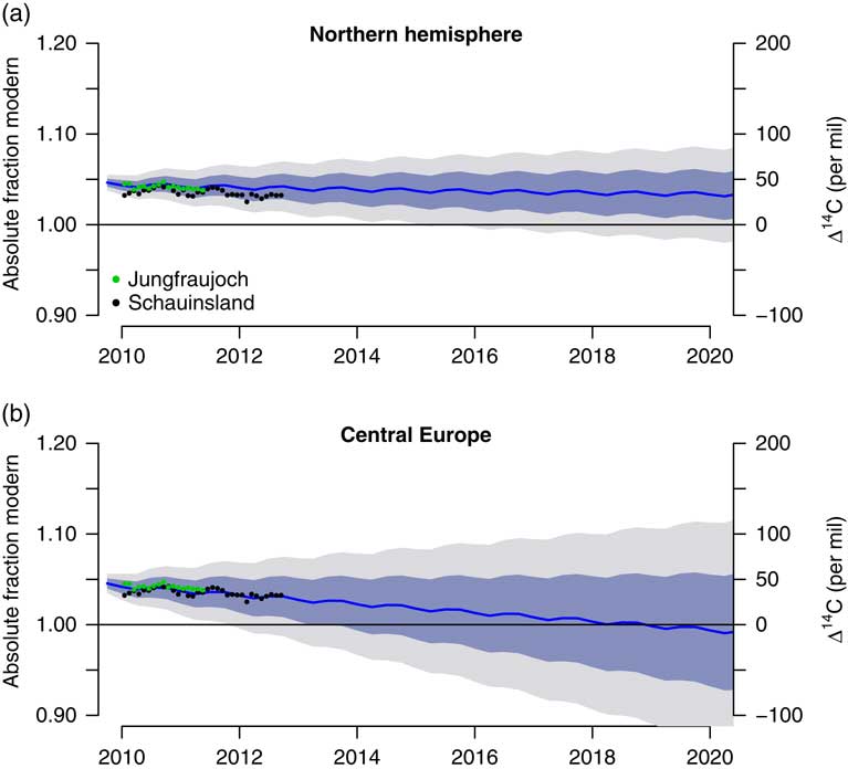
To predict the decline in atmospheric radiocarbon for central Europe based on the Jungfraujoch and Schauinsland stations, I ran a forecast selecting the ETS model that best matches the observations reported in Levin et al. (Reference Levin, Kromer and Hammer2013) (Figure 4b). In this forecast, the rate of radiocarbon decline is faster, and mean atmospheric radiocarbon crosses the Δ14C=0 per mil threshold much earlier.
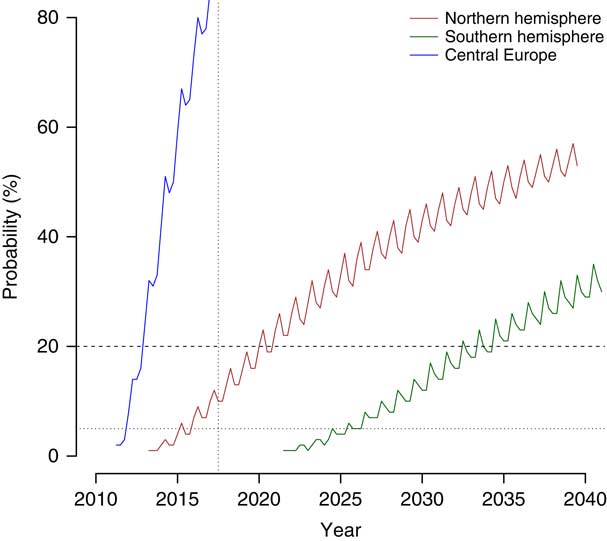
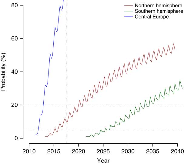
Atmospheric radiocarbon is expected to return to pre-1950s levels within the next decades with different probabilities for the different hemispheres. Values of Δ14C≤0‰ are within 95% prediction intervals of the forecast starting as early as 2016 for the northern hemisphere, and 2025 for the southern hemisphere. For central Europe, it is very likely (>90% probability) that the Δ14C≤0‰ threshold is being crossed by summer 2018.
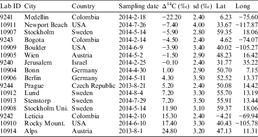
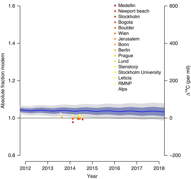
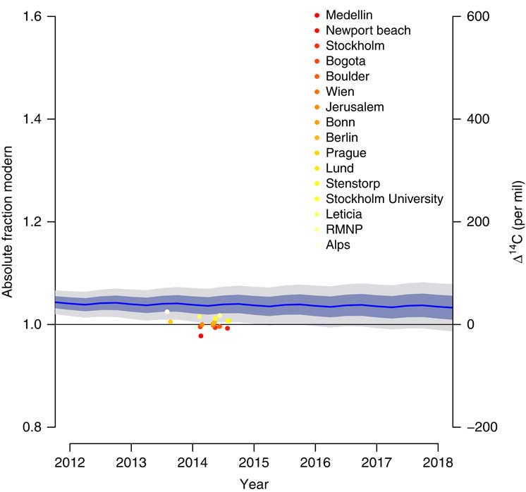
Although the hemispheric averages of background air are expected to return to pre-1950 levels within the next decades, this threshold has been already crossed locally in major cities around the world (Figure 6, Table 2). Air in metropolitan areas with high fossil-fuel emission levels such as Medellín, Stockholm, and the Newport Beach area in California show the highest influence of fossil-fuel derived carbon. Air in European cities such as Berlin and Prague had not crossed the pre-1950 level yet, but Jerusalem was in the limit in 2014 (−0.1±2.4 per mil). As expected, the high altitude samples from the Austrian Alps are very close to the forecasted global values, whereas the samples from Rocky Mountain National Park were much below the forecasted global average, but within the 95% prediction interval of the forecast.
Radiocarbon measured in annual plants (mostly Taraxacum spp.) collected across different cities and natural areas.

DISCUSSION
The time series decomposition presented here shows properties of the trend, slope, and seasonality of atmospheric radiocarbon for different hemispheric zones that complements previous analyses based on sets of individual stations (Levin et al. Reference Levin, Naegler, Kromer, Diehl, Francey, Gomez-Pelaez, Steele, Wagenbach, Weller and Worthy2010; Graven et al. Reference Graven, Guilderson and Keeling2012; Levin et al. Reference Levin, Kromer and Hammer2013) and global carbon models (Caldeira et al. Reference Caldeira, Rau and Duffy1998; Randerson et al. Reference Randerson, Enting, Schuur, Caldeira and Fung2002; Turnbull et al. Reference Turnbull, Rayner, Miller, Naegler, Ciais and Cozic2009; Levin et al. Reference Levin, Naegler, Kromer, Diehl, Francey, Gomez-Pelaez, Steele, Wagenbach, Weller and Worthy2010; Graven Reference Graven2015). One main advantage of this analysis is the use of the harmonized series compiled by Hua et al. (Reference Hua, Barbetti and Rakowski2013), which provide a spatial average across the different stations from which atmospheric radiocarbon has been measured. The series also resolve issues of temporal gaps for the individual stations, and give a comprehensive overview of the dynamic behavior of atmospheric radiocarbon in background air during the past 40 years for the two hemispheres.
The series decomposition analyses showed that the overall decline of atmospheric radiocarbon was higher in the northern hemisphere than in the southern hemisphere. This is not surprising because the large levels of fossil-fuel emissions in the northern hemisphere are expected to significantly dilute atmospheric radiocarbon (Levin et al. Reference Levin, Schuchard, Kromer and Muennich1989, Reference Levin, Naegler, Kromer, Diehl, Francey, Gomez-Pelaez, Steele, Wagenbach, Weller and Worthy2010; Turnbull et al. Reference Turnbull, Rayner, Miller, Naegler, Ciais and Cozic2009; Graven et al. Reference Graven, Guilderson and Keeling2012). Rates of decline since 2005 have been below −5 per mil per year. This implies that if rates of decline continue decreasing, they may pose significant challenges for detecting annual trends in atmospheric radiocarbon given that the uncertainty in new generation AMS systems is between 3 to 2 per mil (Synal et al. Reference Synal, Stocker and Suter2007; Wacker et al. Reference Wacker, Bonani, Friedrich, Hajdas, Kromer, Nĕmec, Ruff, Suter, Synal and Vockenhuber2010).
Atmospheric radiocarbon is expected to return to pre-1950 levels in the northern hemisphere by 2020, the year predicted by Caldeira et al. (Reference Caldeira, Rau and Duffy1998), with a probability ~20% (Figure 5). In the southern hemisphere however, it is unlikely that atmospheric radiocarbon reach values below 0 per mil by 2020. Based on more recent observations from central Europe, the pre-1950 threshold may be crossed with high probability (>90%) by summer 2018 (Figure 5).
Probability of Δ14C≤0‰ for the different hemispheric zones calculated as 100 minus different probability levels of the lower prediction interval for each forecast time. As a reference, 20 and 5% probability levels are presented in dashed and dotted lines, respectively. The vertical dotted line represents July 2018.
It is not possible to attribute any particular process that may contribute to the observed trends in the data with this statistical approach. However, previous analyses (Caldeira et al. Reference Caldeira, Rau and Duffy1998; Randerson et al. Reference Randerson, Enting, Schuur, Caldeira and Fung2002; Levin et al. Reference Levin, Kromer and Hammer2013; Currie et al. Reference Currie, Brailsford, Nichol, Gomez, Sparks, Lassey and Riedel2011) may help to explain some of the properties of the observed time series. For instance, different processes are responsible for determining atmospheric radiocarbon content: fossil fuel emissions, ocean-atmosphere exchange, stratosphere-troposphere mixing, terrestrial ecosystem fluxes, emissions from nuclear industry, and cosmogenic production (Oeschger et al. Reference Oeschger, Siegenthaler, Schotterer and Gugelmann1975; Randerson et al. Reference Randerson, Enting, Schuur, Caldeira and Fung2002; Naegler and Levin Reference Naegler and Levin2006; Levin et al. 2010; Graven Reference Graven2015). The recent slower rates of decline in the northern hemisphere may be explained by the contribution of the terrestrial biosphere and oceans that return decades-old bomb radiocarbon and therefore counterbalance the effect of increased fossil fuel emissions (Caldeira et al. Reference Caldeira, Rau and Duffy1998; Randerson et al. Reference Randerson, Enting, Schuur, Caldeira and Fung2002; Currie et al. Reference Currie, Brailsford, Nichol, Gomez, Sparks, Lassey and Riedel2011). For the southern hemisphere, ocean-atmosphere exchange plays a larger role, and the slow in radiocarbon decline in recent years may be explained by return of bomb radiocarbon by the mixed layer (Currie et al. Reference Currie, Brailsford, Nichol, Gomez, Sparks, Lassey and Riedel2011).
The combined effect of terrestrial biosphere, ocean exchange, fossil-fuel emissions as well as horizontal and vertical air transport may have an important contribution in reducing the amplitude of the seasonal cycle (Levin et al. Reference Levin, Naegler, Kromer, Diehl, Francey, Gomez-Pelaez, Steele, Wagenbach, Weller and Worthy2010). The best ETS model identified here predicts the seasonal cycle as proportional to the trend term; i.e. the higher the amount of radiocarbon in the atmosphere the higher the amplitude of the seasonal cycle, and as radiocarbon content decline in both hemispheres so does its seasonality. Given that the growth term of the series had stabilized in the recent decade, the amplitude of the seasonal cycle had remained constant in the last part of the curve. These results are consistent with model predictions by Randerson et al. (Reference Randerson, Enting, Schuur, Caldeira and Fung2002), who predicted a decline in seasonality over time due to decrease in seasonality in ocean and terrestrial biosphere exchange, with strong contributions from fossil-fuel signals.
Caldeira et al. (Reference Caldeira, Rau and Duffy1998), and more recently Graven (Reference Graven2015), predicted that in a business-as-usual scenario of fossil-fuel emissions, radiocarbon content would return to pre-1950 levels by ~2020. Current trajectories of atmospheric radiocarbon seem to agree with this prediction, but with important differences among hemispheric regions. The Δ14C≤0‰ threshold would be crossed in the northern hemisphere with higher probability than in the southern hemisphere, which may be a consequence of differences in contributions between the terrestrial biosphere and the oceans, the later being more relevant for the southern hemisphere. It is also likely that the rate of decline of atmospheric radiocarbon in the northern hemisphere may increase in the future (become more negative) if the previously sequestered bomb-radiocarbon is exhausted, and then fossil-fuel derived carbon may have a larger influence in the northern hemisphere. This is clearly illustrated in the urban areas we analyzed where fossil-fuel emissions dominate over terrestrial exchange and therefore radiocarbon is close or have already crossed the Δ14C≤0‰ threshold.
The forecasted atmospheric radiocarbon curves presented here may be useful for different studies where data on the atmospheric background is not available after the latest release of the compiled curves (Hua et al. Reference Hua, Barbetti and Rakowski2013). The methodology of time-series decomposition and forecast may also be useful to produce forecasts for individual stations or for new releases of compiled curves. However, care must be taken in using these forecasts in different applications, and prediction uncertainties must always be considered. Possible changes in the rates of decline of atmospheric radiocarbon for the different hemispheres may deviate in the future from the rates calculated in the time-series decomposition presented here. Therefore, these forecasted radiocarbon trends must be used with caution.
Forecasted northern hemisphere atmospheric radiocarbon values (with 68 and 95% prediction intervals), superimposed with radiocarbon values measured in plants growing on different industrial cities and remote areas without fossil fuel influence. This radiocarbon value represents the mix of fossil-fuel derived carbon and the mixing with background air.
ACKNOWLEDGMENTS
Funding was provided by the Max Planck Society and the German Research Foundation through the Emmy-Noether programme (SI 1953/2-1).
SUPPLEMENTARY MATERIAL
To view supplementary material for this article, please visit https://doi.org/10.1017/RDC.2018.33