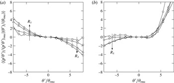
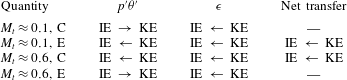
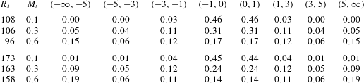
1. Introduction
Understanding the effect of compressibility in turbulent flows is important in many areas of scientific and engineering interest, such as the design of supersonic vehicles, the mixing in high speed flows and astrophysical phenomena, among others. Common features that distinguish compressible flows from their incompressible counterparts include the presence of fluctuations of thermodynamic variables and the non-zero dilatation values of the fluid medium. Hence, in order to better understand the nature of compressible flows, it is common to study the behaviour of thermodynamic variables, the changes that the dilatation of fluid elements bring about and how they are interrelated.
The general disposition towards accounting for compressibility effects has been to decompose the velocity field into incompressible (solenoidal) and compressible (dilatational) components based on Helmholtz decomposition. A similar form of decomposition has been extended, though in a more ambiguous manner, to pressure. Other attempts have also been made to isolate compressibility effects. For instance, Kovasznay (Reference Kovasznay1953) linearized the Navier–Stokes equations to obtain solutions as superposition of vorticity, entropy and acoustic modes under the assumption that the effects of compressibility are very small. Chu & Kovásznay (Reference Chu and Kovásznay1958) extended the analysis as a second-order approximation to account for stronger compressibility effects. Dastgeer & Zank (Reference Dastgeer and Zank2005) employed a similar approach and found that density and temperature are anti-correlated for fluids in the interstellar medium. The linear assumption, however, is very restrictive for a large class of engineering flows that operate at high speeds where different high-amplitude modes interact and thus superposition may not be always appropriate.
Thermodynamic variables, which are related by an equation of state, are typically coupled to hydrodynamics leading to acoustic phenomena, such as, propagation of sound waves. Depending on the level of compressibility, which is commonly quantified by the turbulent Mach number (
 $M_{t}=\langle u_{i}u_{i}\rangle ^{1/2}/\langle c\rangle$
, summation implied and
 $\langle X\rangle$
represents a suitably defined average of the variable
 $X$
), different approximations can be made that lead to distinct flow regimes. For instance, at low
 $M_{t}$
, the acoustic time scale is much smaller than the convective and viscous time scales leading to a simplified set of equations (Erlebacher et al.
Reference Erlebacher, Hussaini, Kreiss and Sarkar1990; Sarkar et al.
Reference Sarkar, Erlebacher, Hussaini and Kreiss1991). This results in a flow regime known as the low-Mach number quasi-isentropic regime, where the flow is characterized by small dilatational fluctuations (Sagaut & Cambon Reference Sagaut and Cambon2008). At higher levels of compressibility, the dilatational fluctuations may be substantial and cannot be neglected. This flow regime, with stronger dilatational fluctuations but with a Mach number still less than unity, is classified as the nonlinear subsonic regime and is the principal regime of investigation here.
Because in compressible flows energy can be either in the form of kinetic or internal energy, there has been significant interest in energy exchanges in compressible flows in general (Miura & Kida Reference Miura and Kida1995; Bataille, Zhou & Bertoglio Reference Bataille, Zhou and Bertoglio1997), shock turbulence interactions (Lee, Lele & Moin Reference Lee, Lele and Moin1993) and in reacting flows (Livescu, Jaberi & Madnia Reference Livescu, Jaberi and Madnia2002). To examine the energy transfer processes, it is useful to take the dot-product of the Navier–Stokes equations with the velocity vector
 $\boldsymbol{u}$
, and then average, which after rearrangements results in an evolution equation for the mean turbulent kinetic energy,
 $\langle \mathscr{K}\rangle$
. This equation, along with the mean internal energy (
 $\langle {\it\rho}e\rangle$
) which expresses conservation of energy can be written, for statistically homogeneous flows, as:
 $$\begin{eqnarray}\displaystyle & \displaystyle \frac{\partial \langle \mathscr{K}\rangle }{\partial t}=\langle p^{\prime }{\it\theta}^{\prime }\rangle -\langle {\it\epsilon}\rangle +\langle \,f_{i}u_{i}\rangle , & \displaystyle\end{eqnarray}$$
 $$\begin{eqnarray}\displaystyle & \displaystyle \frac{\partial \langle {\it\rho}e\rangle }{\partial t}=-\langle p^{\prime }{\it\theta}^{\prime }\rangle +\langle {\it\epsilon}\rangle -{\it\Lambda}. & \displaystyle\end{eqnarray}$$
 $\langle p^{\prime }{\it\theta}^{\prime }\rangle$
(primes in variables represent fluctuations around the mean) and
 $\langle {\it\epsilon}\rangle$
are the mean pressure-dilatation correlation and dissipation rate, which as is clearly seen, represent exchange terms between the two energy modes. The term
 $\langle \,f_{i}u_{i}\rangle$
is the mean energy injected into the system (to be described formally below) and
 ${\it\Lambda}$
is the amount of energy removed from the system. Equations (1.1) and (1.2) form the basis of our present work. We study the scaling of the terms in these equations with
 $R_{{\it\lambda}}$
and
 $M_{t}$
and the nature of energy exchange between the internal and kinetic energies.
One of the simplest frameworks to investigate these fundamental processes is in homogeneous isotropic turbulence where wall effects and anisotropy are not present (Ishihara, Gotoh & Kaneda Reference Ishihara, Gotoh and Kaneda2009). Recent advances in computing have enabled large-scale simulations of homogeneous compressible turbulence at grid resolutions as high as
 $1024^{3}$
(Petersen & Livescu Reference Petersen and Livescu2010; Wang et al.
Reference Wang, Shi, Wang, Xiao, He and Chen2012). Using some of the most powerful supercomputers available today, we report results from simulations of homogeneous forced compressible isotropic turbulence with grid resolutions ranging from
 $64^{3}$
to
 $2048^{3}$
for Taylor Reynolds number ranging from
 $38$
to
 $450$
and Mach numbers
 $0.1$
to
 $0.6$
. The database used here comprises that used in Donzis & Jagannathan (Reference Donzis and Jagannathan2013a
) with some simulations extended for statistical convergence as well as new simulations to cover more values of
 $M_{t}$
especially at high resolutions. The
 $2048^{3}$
simulation with a Taylor Reynolds number of
 $450$
is, to the authors knowledge, the largest simulation of forced compressible isotropic turbulence available in the literature (Donzis & Jagannathan Reference Donzis and Jagannathan2013a
). Our focus in this work, however, is on energy exchanges and the scaling of variables involved in this process such as dilatation, pressure-dilatation, dissipation among others.
The rest of the paper is organized as follows. Background on the specific quantities investigated in this work is given in § 2. The computational details and database are described in § 3. Effect of compressibility on classical scaling relations is analysed in § 4 followed by a discussion on equipartition of energy in compressible flows in § 5. Finally, statistics of pressure, its correlation with dilatation and energy transfer dynamics between internal and kinetic energy modes are presented in § 6. Summary and some final remarks are presented in § 7.
2. Background
For homogeneous compressible flows, the Helmholtz decomposition allows the velocity field to be written as,
 $\boldsymbol{u}=\boldsymbol{u}^{\boldsymbol{s}}+\boldsymbol{u}^{\boldsymbol{d}}$
, where
 $\boldsymbol{u}^{\boldsymbol{s}}$
is the solenoidal (
 $\boldsymbol{{\rm\nabla}}\boldsymbol{\cdot }\boldsymbol{u}^{\boldsymbol{s}}=0$
) and
 $\boldsymbol{u}^{\boldsymbol{d}}$
is the dilatational (
 $\boldsymbol{{\rm\nabla}}\times \boldsymbol{u}^{\boldsymbol{d}}=0$
) component of velocity. Compressibility effects have typically been attributed to the often small yet non-negligible contribution from the dilatation field (Lele Reference Lele1994) which is zero in incompressible flows. Thus, in order to understand the effects of compressibility, it is important to delineate the similarities, differences and relative contributions of the solenoidal and dilatational modes and their scaling with the Taylor Reynolds number (
 $R_{{\it\lambda}}=\langle {\it\rho}\rangle \langle u_{i}u_{i}/3\rangle ^{1/2}{\it\lambda}/\langle {\it\mu}\rangle$
, where
 ${\it\lambda}\equiv \langle u^{2}\rangle ^{1/2}/\langle (\partial u/\partial x)\rangle ^{1/2}$
is the Taylor length scale and
 $\langle {\it\mu}\rangle$
is the mean dynamic viscosity) and the turbulent Mach number,
 $M_{t}$
. A fundamental aspect of turbulence is the presence of a wide range of length scales, which typically ranges from the integral scales to the so-called Kolmogorov scale (Kolmogorov Reference Kolmogorov1941). For smaller scales, dissipative effects are assumed to be dominant. Although the Kolmogorov scale has been proposed for incompressible flows, it has been used extensively to understand and characterize compressible flows. However, its scaling has not been assessed systematically in these flows, where concerns may appear especially at high
 $M_{t}$
. We address this in § 4.
The mean energy dissipation rate in incompressible turbulence becomes independent of the fluid viscosity at very high Reynolds numbers. This phenomenon, often known as dissipative anomaly and typically observed as the normalized dissipation rate
 $D\equiv \langle {\it\epsilon}\rangle u^{3}/L$
approaches a constant at high
 $R_{{\it\lambda}}$
, is central to the dynamics of energy cascade and has been supported by experiments and simulations over the past several decades (Sreenivasan Reference Sreenivasan1984, Reference Sreenivasan1998; Kaneda et al.
Reference Kaneda, Ishihara, Yokokawa, Itakura and Uno2003; Donzis, Sreenivasan & Yeung Reference Donzis, Sreenivasan and Yeung2005). Here,
 $L\equiv {\rm\pi}/(2u^{2})\int _{0}^{k_{max}}E(k)/k\,\text{d}k$
, is the integral length scale where
 $k_{max}$
is the highest resolved wavenumber in the simulation. Some theoretical investigations (Shivamoggi Reference Shivamoggi1995, Reference Shivamoggi2005) explored the differences between the asymptotic behaviour of
 $D$
in incompressible and compressible turbulence. However, a systematic assessment (numerical or experimental) of whether
 $D$
asymptotes to a constant at high Reynolds and Mach numbers, and if it does, the value of that constant has not been thoroughly investigated. The mean dissipation rate, like velocity, can be decomposed into solenoidal (
 $\langle {\it\epsilon}^{s}\rangle$
) and dilatational (
 $\langle {\it\epsilon}^{d}\rangle$
) components (Sarkar et al.
Reference Sarkar, Erlebacher, Hussaini and Kreiss1991) and is thus natural to inquire about the asymptotic behaviour of each at high Reynolds numbers. It is important to note that
 $\langle {\it\epsilon}^{s}\rangle$
, although commonly-called incompressible dissipation, may also be affected by compressibility effects in a compressible flow. Thus, dissipative anomaly cannot be, in principle, assumed for either one of the components of dissipation. In fact the model leading to
 $\langle {\it\epsilon}^{d}\rangle \sim M_{t}^{2}\langle {\it\epsilon}^{s}\rangle$
by Sarkar et al. (Reference Sarkar, Erlebacher, Hussaini and Kreiss1991) which was based on a low-Mach number approximation, would suggest a strong Mach number dependence but no Reynolds dependence. Thus if
 $\langle {\it\epsilon}^{s}\rangle$
is asymptotically independent of molecular transport coefficients, so will
 $\langle {\it\epsilon}^{d}\rangle$
though the asymptotic constant would depend on
 $M_{t}$
. We address this in § 4.
The energy dissipation rate discussed above is an irreversible transfer from kinetic to internal energy. There has been substantial interest in understanding, among all modes, what the distribution of energy is. Sarkar et al. (Reference Sarkar, Erlebacher, Hussaini and Kreiss1991) proposed an equipartition of energy between the dilatational components of kinetic energy and potential energy (due to pressure). Their formulation was based on root-mean-square (r.m.s.) quantities to represent energies in different modes, and has been sometimes referred to as the weak equilibrium hypothesis. A more stringent adaptation, the strong equilibrium hypothesis, requires kinetic and potential energies to be in equilibrium with each other for each wavenumber (Sagaut & Cambon Reference Sagaut and Cambon2008). Equipartition between acoustic and vortical modes had been proposed analytically in the literature (Kraichnan Reference Kraichnan1955; Sarkar et al.
Reference Sarkar, Erlebacher, Hussaini and Kreiss1991; Shivamoggi Reference Shivamoggi1997) and has received some support, in the weak-equilibrium sense, in decaying simulations (Lee & Girimaji Reference Lee and Girimaji2013), and also in shear flows (Bertsch, Suman & Girimaji Reference Bertsch, Suman and Girimaji2012) for low
 $M_{t}$
. However, only a few studies have investigated this result for stationary compressible turbulence (Kida & Orszag Reference Kida and Orszag1990; Miura & Kida Reference Miura and Kida1995), which were also at low Reynolds number (
 $R_{{\it\lambda}}\leqslant 40$
). While originally proposed to be valid for low
 $M_{t}$
and high
 $R_{{\it\lambda}}$
, our simulations suggest that equipartition of energy seems to be a good approximation at high
 $M_{t}$
too in the case of stationary turbulence.
The other exchange term in (1.1) and (1.2), is the correlation between pressure and dilatation, often known as pressure-dilatation correlation (
 $p^{\prime }{\it\theta}^{\prime }$
). While the mean dissipation rate represents a uni-directional energy transfer from kinetic to internal energy modes, the pressure-dilatation correlation facilitates a bi-directional energy exchange mechanism between them. It is also clear, from (1.1) and (1.2), that any influence of compressibility in pressure fluctuations could bring about changes in the pressure-dilatation correlation and consequently the way energy is exchanged, affecting the global dynamics of the flow. We examine some existing scaling relations for the solenoidal and dilatation components of pressure and identify departures, if any. For example, the probability density function (p.d.f.) of pressure, is known to be negatively skewed in incompressible flows (Holzer & Siggia Reference Holzer and Siggia1993; Pumir Reference Pumir1994; Vedula & Yeung Reference Vedula and Yeung1999). In an earlier study (Donzis & Jagannathan Reference Donzis and Jagannathan2013a
), we found that at high
 $M_{t}$
, the p.d.f. becomes positively skewed following a log-normal distribution for positive fluctuations. Here, though our main concern is in energy distributions and exchanges, we are also able to show that this qualitative change in the p.d.f. of pressure is the result of large contributions of dilatational pressure.
While in incompressible turbulence the role of pressure is restricted to redistribution of energy across components of momentum by upholding continuity, in compressible turbulence pressure couples both thermodynamics and hydrodynamics. Due to this coupling, it is natural to expect any change in hydrodynamics, like dilatation of the fluid, to affect the thermodynamic fluctuations. For example, as we show below, regions of high pressure and strong expansions tend to co-exist at high
 $M_{t}$
. Furthermore, unlike in incompressible turbulence, the correlation between regions of low/high pressure and enstrophy decreases with increasing Mach number, and thus the skewness of pressure at high
 $M_{t}$
cannot be attributed to solenoidal motions.
The effects of strong fluid dilatation have been studied before (Samtaney, Pullin & Kosovic Reference Samtaney, Pullin and Kosovic2001; Pirozzoli & Grasso Reference Pirozzoli and Grasso2004; Wang et al.
Reference Wang, Shi, Wang, Xiao, He and Chen2011, Reference Wang, Shi, Wang, Xiao, He and Chen2012), where it is argued that the appearances of these intense events tend to increase with
 $M_{t}$
. These studies also indicate as
 $M_{t}$
increases strong compressions are more likely to occur than equally strong expansions which we also quantify for a range of
 $R_{{\it\lambda}}$
and
 $M_{t}$
in § 6.3. While it is generally believed that a strong compression of fluid increases the energy dissipation (Lee, Lele & Moin Reference Lee, Lele and Moin1991; Lee, Girimaji & Kerimo Reference Lee, Girimaji and Kerimo2009) triggering transfers from kinetic to internal mode, it is still not well established if a similar picture holds true for equally strong expansions. Moreover, the net transfer between kinetic and internal energies can change due to the contribution from pressure-dilatation correlation. We discuss the net energy exchanges in regions of high positive and negative dilatation in § 6.
3. Numerical simulations and database
3.1. Computational details
Turbulence is governed by the Navier–Stokes equations representing the conservation of mass, momentum and energy,
 $$\begin{eqnarray}\displaystyle & \displaystyle \frac{\partial {\it\rho}}{\partial t}+\frac{\partial }{\partial x_{i}}({\it\rho}u_{i})=0, & \displaystyle\end{eqnarray}$$
 $$\begin{eqnarray}\displaystyle & \displaystyle \frac{\partial }{\partial t}({\it\rho}u_{i})+\frac{\partial }{\partial x_{j}}({\it\rho}u_{i}u_{j})=-\frac{\partial p}{\partial x_{i}}+\frac{\partial }{\partial x_{j}}({\it\sigma}_{ij})+{\it\rho}f_{i}, & \displaystyle\end{eqnarray}$$
 $$\begin{eqnarray}\displaystyle & \displaystyle \frac{\partial }{\partial t}({\it\rho}e)+\frac{\partial }{\partial x_{i}}({\it\rho}eu_{i})=-p\frac{\partial u_{i}}{\partial x_{i}}+\frac{\partial }{\partial x_{i}}\left({\it\kappa}\frac{\partial T}{\partial x_{i}}\right)+{\it\sigma}_{ij}\unicode[STIX]{x1D61A}_{ij}-{\it\Lambda}. & \displaystyle\end{eqnarray}$$
 ${\it\rho}$
is density,
 $u_{i}$
is the
 $i$
th component of velocity,
 $p$
is pressure,
 $e$
is internal energy per unit mass,
 $T$
is temperature,
 ${\it\kappa}$
is thermal conductivity and
 $f_{i}$
is the external forcing. The viscous stress tensor,
 ${\it\sigma}_{ij}$
, and strain rate tensor,
 $\unicode[STIX]{x1D61A}_{ij}$
, are given by,
 $$\begin{eqnarray}\displaystyle & \displaystyle {\it\sigma}_{ij}={\it\mu}\left(\frac{\partial u_{i}}{\partial x_{j}}+\frac{\partial u_{j}}{\partial x_{i}}-\frac{2}{3}{\it\delta}_{ij}\frac{\partial u_{k}}{\partial x_{k}}\right), & \displaystyle\end{eqnarray}$$
 $$\begin{eqnarray}\displaystyle & \displaystyle \unicode[STIX]{x1D61A}_{ij}=\frac{1}{2}\left(\frac{\partial u_{i}}{\partial x_{j}}+\frac{\partial u_{j}}{\partial x_{i}}\right). & \displaystyle\end{eqnarray}$$
 $\boldsymbol{f}$
in the momentum equations, in order to maintain a stationary state energy needs to be removed from the system. This is accomplished through an additional term,
 ${\it\Lambda}$
, in the energy equation (3.3). This can be done in several ways as discussed in § 3.2. In order to close the set of equations, we consider an ideal gas that follows the equation of state,
 $$\begin{eqnarray}p={\it\rho}RT,\end{eqnarray}$$
where
 $R$
is the gas constant of the fluid.
The equations are solved in conservative form using compact schemes (Lele Reference Lele1992) with periodic boundary conditions in all three spatial directions. In order to control aliasing errors, nonlinear terms are computed using a skew-symmetric form (Blaisdell, Mansour & Reynolds Reference Blaisdell, Mansour and Reynolds1993). Compact schemes have a very high resolving efficiency compared to conventional finite difference schemes and, unlike spectral schemes, are more amenable to more complex geometries involving different types of boundary conditions. Formally, the derivative
 $g^{\prime }$
of a function
 $g$
is approximated by,
 $\sum _{j=-m}^{m}{\it\alpha}_{j}g_{i+j}^{\prime }=\sum _{j=-n}^{n}a_{j}g_{i+j}$
, where
 $m$
,
 $n$
define the stencil size and
 ${\it\alpha}_{j},a_{j}$
are the coefficients of the stencil for the derivative and function. This leads to a system of linear equations of the form
 $\unicode[STIX]{x1D648}\boldsymbol{g}^{\prime }=\unicode[STIX]{x1D63C}\boldsymbol{g}$
, where
 $\unicode[STIX]{x1D648}$
is a banded matrix. A family of schemes is obtained by varying
 $m$
and
 $n$
. Specifically, for
 $m=2$
,
 $n=3$
a tenth-order scheme is obtained, which requires solving a penta-diagonal system. This can be solved efficiently using highly optimized mathematical libraries in
 $\mathit{O}(59N)$
operations (Lv & Le Reference Lv and Le2008). The code, which leverages the spectral-like accuracy of compact schemes, is parallelized using a hybrid MPI-OpenMP technique. The domain is decomposed in two directions which enables the utilization of up-to
 $N^{2}$
processors for a problem size of
 $N^{3}$
. For problems of current interest where
 $N=2048$
, a maximum of
 $2048^{2}$
processing cores can be used which is beyond the largest supercomputing facilities available currently, but may be available in so-called exascale computing.
The derivatives can be efficiently computed when one processor has all the data along the direction in which the derivative is sought. This ‘pencil’ of data is initially aligned, say, with
 $x$
. All the terms involving derivatives in the
 $x$
direction are then computed. However, in order to compute the entire right-hand side of the Navier–Stokes equations, derivatives along the other two directions are required. There are two options for computing these derivatives: (i) by halo exchanges along the processor boundaries, (Cook et al.
Reference Cook, Cabot, Williams, Miller, Supinski, de Yates and Welcome2005) or (ii) by transposition of data from
 $x$
to
 $y$
and subsequently
 $y$
to
 $z$
pencils (Jagannathan & Donzis Reference Jagannathan and Donzis2012). While both methods have been shown to scale well at core counts of
 $\mathit{O}(10^{4})$
, the latter is independent of the order of accuracy and facilitates overlapping of communication and computation and has been used for this work. Once the derivatives are computed, the variables are marched in time using a third-order low-storage Runge–Kutta scheme. For the following time step, the order of transposition is inverted to save one transpose per variable every other step.
The code has shown very good scaling up to 524, 288 cores on grid resolutions up to
 $4096^{3}$
. Small departures from ideal scaling are seen only at very large core counts, where the memory footprint is of the order of cache size and hence latency effects, which can be attributed to communication, tend to overwhelm the computational time. Employing an additional level of parallelism based on shared memory alongside message passing techniques has decreased the communication time by as much as 30 %. The implementation, benchmarks, and other diagnostic methods are described in Jagannathan & Donzis (Reference Jagannathan and Donzis2012).
3.2. Simulation database
Direct numerical simulations (DNS) at different Reynolds and Mach number are required, for instance, to predict asymptotes at high Reynolds number and assess effects of compressibility. We use a large database of homogeneous forced isotropic compressible turbulence (Donzis & Jagannathan Reference Donzis and Jagannathan2013b ) to investigate the Reynolds and Mach number scaling of solenoidal and dilatational components of several quantities, effects of dilatation on thermodynamic quantities and the dynamics of energy transfer between internal and kinetic modes. Some of the simulations in the database have been extended for a longer duration to decrease statistical variability.
In order to maintain a stationary state, energy is injected at the large scales through the momentum equations, a technique that has been used extensively in incompressible (Eswaran & Pope Reference Eswaran and Pope1988; Yeung & Brasseur Reference Yeung and Brasseur1991; Overholt & Pope Reference Overholt and Pope1998; Rosales & Meneveau Reference Rosales and Meneveau2005) and in compressible flows (Kida & Orszag Reference Kida and Orszag1990; Petersen & Livescu Reference Petersen and Livescu2010; Wang et al.
Reference Wang, Shi, Wang, Xiao, He and Chen2012). Forcing in compressible turbulence, however, has a much wider and interdependent parameter space because the forcing parameters (mean temperature
 $T_{0}$
, number of forced wavenumbers
 ${\it\kappa}_{f}$
, amplitude of forcing, extent of solenoidal or dilatational forcing and time scale of forcing) are used to control not only the Reynolds number but also the turbulent Mach number which in turns depends on e.g. the mean temperature. Each of these parameters may affect the flow variables simultaneously. For instance, if
 $T_{0}$
is decreased, we might expect
 $M_{t}$
to increase (
 $M_{t}\propto u/\sqrt{T}$
), but it could also change
 ${\it\mu}$
thus affecting the Reynolds number as well. This interplay of parameters compounded by constraints of achieving (i) well-resolved simulations (
 $k_{max}{\it\eta}\approx 1.5$
, to be shown later), (ii) the integral length scale being a fraction of the domain size, and (iii) the maximum
 $R_{{\it\lambda}}$
for a given grid resolution, makes it a difficult problem to conduct a parametric variation of
 $R_{{\it\lambda}}$
and
 $M_{t}$
. This may account for why investigations of forced compressible turbulence have been scarce compared to incompressible turbulence.
We have implemented a low-wavenumber stochastic forcing based on Eswaran & Pope (Reference Eswaran and Pope1988), that acts on wavenumbers (
 ${\it\kappa}$
) inside a spherical shell of radius
 ${\it\kappa}_{f}$
(
 ${\it\kappa}\leqslant {\it\kappa}_{f},{\it\kappa}_{f}=3$
). Stochastic forcing for compressible flows have been used before, though it has been limited to, e.g., a single wavenumber (Kida & Orszag Reference Kida and Orszag1990). In this work, the forcing term in (3.2) is given by the vector
 $$\begin{eqnarray}\boldsymbol{f}=\mathop{\sum }_{|\boldsymbol{k}|<k_{f}}\hat{\boldsymbol{f}}_{\bot }(\boldsymbol{k})\text{e}^{-\text{i}\boldsymbol{k}\boldsymbol{\cdot }\boldsymbol{x}},\end{eqnarray}$$
where
 $\hat{\boldsymbol{f}}_{\bot }(\boldsymbol{k})$
is the projection onto the plane perpendicular to the wavenumber vector (which assures purely solenoidal forcing) of a random vector constructed using six independent integrated Uhlenbeck–Ornstein random processes. The injected energy cascades by nonlinear interactions and is dissipated at the small scales. Since this increases the total energy of the system, one has to devise a mechanism to remove energy to maintain a stationary state. We have implemented this in two different ways: by removing energy (i) such that the mean internal energy is constant and (ii) homogeneously and with a value equal to the average energy input at every step. Consistent with previous studies (Wang et al.
Reference Wang, Wang, Xiao, Shi and Chen2010) results are virtually unaffected by the specific means in which energy is removed from the system. The temperature dependence of viscosity and diffusivity (for scalars) follow a power-law dependence with an exponent of 0.5, and the fluid is assumed to be an ideal gas with a Prandtl number,
 $Pr$
of
 $0.72$
. The relative difference between different temperatures dependencies of viscosity used in the literature is only a few percentage points (Wang et al.
Reference Wang, Wang, Xiao, Shi and Chen2010) and the conclusions here are, thus, unaffected by the specific choice of the exponent as our own tests confirm.
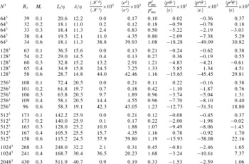
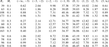
While it is possible to force independently both the solenoidal and dilatational mode of velocity, in this work, our focus will be in simulations where only the solenoidal mode is forced. The main reason for this choice is to study dilatational motions as they emerge from Navier–Stokes dynamics as opposed to those imposed by external factors such as dilatational forcing. The DNS database, summarized in table 1, consists of grid resolutions from
 $64^{3}$
to
 $2048^{3}$
with Taylor Reynolds number ranging from 38 to 450 at different Mach numbers,
 $M_{t}=0.1,0.2,0.3,0.4$
and
 $0.6$
. The table includes basic information about integral and Taylor length scales as well as the ratio of dilatational to solenoidal kinetic energy, dissipation rate, and pressure.
Simulation database: number of grid points (
 $N^{3}$
), Reynolds and Mach numbers (
 $R_{{\it\lambda}}$
and
 $M_{t}$
), normalized integral and Taylor length scales, ratio of dilatational to solenoidal kinetic energy, dissipation and r.m.s. of pressure, ratio of mean pressure-dilatation correlation to mean dissipation, as well as the solenoidal and dilatational pressure-dilatation correlation to mean dissipation.

To ensure accurate small-scale resolution, we have done convergence studies. We first note that while strong compressions (so-called ‘shocklets’) may in principle impose further constraints in resolution, it has been suggested that the most probable shock thickness is of the order of the mean Kolmogorov scale (Samtaney et al. Reference Samtaney, Pullin and Kosovic2001). Furthermore, even the strongest shocklets have been suggested to be comparable to the strongest velocity gradients found in incompressible turbulence due to intermittency (Donzis & Jagannathan Reference Donzis and Jagannathan2013b ). This suggests that the resolution criterion may not be much stricter than in well-resolved incompressible DNS. Still, since these are theoretical results based on strong assumptions, it is important to assess accuracy based on numerical data.
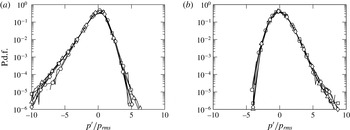
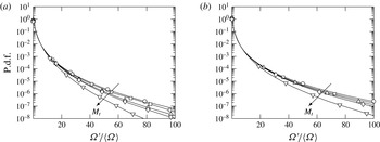
P.d.f. of pressure fluctuations normalized at
 $R_{{\it\lambda}}\approx 60$
for (a)
 $M_{t}\approx 0.1$
(b)
 $M_{t}\approx 0.6$
. Symbols represent
 ${\it\eta}/{\rm\Delta}x\approx 0.125$
(○),
 $0.25$
(▫),
 $0.50$
(▵),
 $1.0$
(♢).

It is also known that the resolution requirement typically depends on the quantity of interest (Watanabe & Gotoh Reference Watanabe and Gotoh2007; Donzis, Yeung & Pekurovsky Reference Donzis, Yeung and Pekurovsky2008a
). Since our main interest is in the effect of thermodynamic variables and dilatation of the flow, we consider pressure and higher-order moments of velocity gradients as our convergence criteria. The p.d.f. of pressure is shown in figure 1 at
 $R_{{\it\lambda}}\approx 60$
and
 $M_{t}~\approx ~0.1$
and 0.6 for different grid resolutions. While the shape of the p.d.f. differs for different
 $M_{t}$
(see § 6 for detailed analysis), the p.d.f.s themselves are converged even at
 ${\it\eta}/{\rm\Delta}x\approx 0.25$
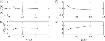
showing little sensitivity to small-scale resolution. High-order moments of velocity gradients, on the other hand, are more sensitive than other quantities such as correlations and spectra (Donzis, Yeung & Sreenivasan Reference Donzis, Yeung and Sreenivasan2008b
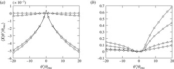
). In figure 2 we show these moments up to order
 $4$
. At low
 $M_{t}$
(
 ${\approx}0.1$
), both third and fourth-order moments are converged at
 ${\it\eta}/{\rm\Delta}x\approx 0.5$
. Indeed, we have verified that moments up to order three are converged when
 ${\it\eta}/{\rm\Delta}x\approx 0.5$
for all Mach numbers in the database. We note, however, that the fourth-order moment at the highest
 $M_{t}$
(
 ${\approx}0.6$
) shows a slight increase at
 ${\it\eta}/{\rm\Delta}x\approx 1$
, which may suggest a more stringent resolution requirement. For all other Mach numbers, however, fourth-order moment are converged. Thus, for the results shown in this paper, a resolution of
 ${\it\eta}/{\rm\Delta}x\approx 0.5$
is found to be sufficient. This seems consistent with the results of Samtaney et al. (Reference Samtaney, Pullin and Kosovic2001) where it was estimated that the most probable shocklet thickness is a few times larger than the Kolmogorov scale. Thus, resolving Kolmogorov scales would also provide enough resolution for shocklets. The convergence seen in figure 2 and other conditions in our database seems to support this conclusion.
Normalized moments of longitudinal velocity gradients,
 $X=(\partial u_{i}/\partial x_{i})/3$
, at
 $R_{{\it\lambda}}\approx 60$
for
 $M_{t}\approx 0.1$
(a,c) and
 $M_{t}\approx 0.6$
(b,d) for different
 ${\it\eta}/{\rm\Delta}x$
. The error bars correspond to a 95 % confidence interval.

3.3. Solenoidal and dilatational components
As mentioned before, the velocity field is decomposed into solenoidal and dilatational field, for which we will use superscripts
 $s$
and
 $d$
respectively. This decomposition is unique for homogeneous flows. Since
 $\boldsymbol{u}^{\boldsymbol{s}}$
and
 $\boldsymbol{u}^{\boldsymbol{d}}$
are orthogonal to each other on the average
 $(\langle \boldsymbol{u}^{\boldsymbol{s}}\boldsymbol{\cdot }\boldsymbol{u}^{\boldsymbol{d}}\rangle =0)$
, respective kinetic energies are related as
 $\langle \mathscr{K}\rangle =\langle \mathscr{K}^{s}\rangle +\langle \mathscr{K}^{d}\rangle$
(Kida & Orszag Reference Kida and Orszag1990; Lele Reference Lele1994), where the solenoidal and dilatational components of mean kinetic energy is given by
 $\langle \mathscr{K}^{s}\rangle =\langle {\it\rho}\boldsymbol{u}_{i}^{\boldsymbol{s}}\boldsymbol{u}_{i}^{\boldsymbol{s}}/2\rangle$
and
 $\langle \mathscr{K}^{d}\rangle =\langle {\it\rho}\boldsymbol{u}_{i}^{\boldsymbol{d}}\boldsymbol{u}_{i}^{\boldsymbol{d}}/2\rangle$
, with summation implied on
 $i$
. Using Reynolds decomposition, we decompose a random variable
 $X$
into mean
 $\langle X\rangle$
and fluctuations
 $X^{\prime }$
, such that
 $X=\langle X\rangle +X^{\prime }$
. For quantities with zero mean, the primes are dropped for simplicity in notation. Two examples are the velocity field
 $u$
and forcing term
 $f$
.
Sarkar et al. (Reference Sarkar, Erlebacher, Hussaini and Kreiss1991) proposed a way to decompose
 $\langle {\it\epsilon}\rangle$
into a solenoidal (
 $\langle {\it\epsilon}^{s}\rangle$
) and dilatational (
 $\langle {\it\epsilon}^{d}\rangle$
) component by recasting them in terms of fluctuating vorticity (
 ${\it\omega}_{i}$
) and dilatation (
 ${\it\theta}$
). Here we use
 $$\begin{eqnarray}\langle {\it\epsilon}^{s}\rangle =\langle {\it\mu}{\it\omega}_{i}{\it\omega}_{i}\rangle ,\quad \langle {\it\epsilon}^{d}\rangle ={\textstyle \frac{4}{3}}\langle {\it\mu}{\it\theta}^{2}\rangle .\end{eqnarray}$$
Note that if the fluctuations in
 ${\it\mu}$
are small, one can write (Sarkar et al.
Reference Sarkar, Erlebacher, Hussaini and Kreiss1991)
 $\langle {\it\mu}{\it\omega}_{i}{\it\omega}_{i}\rangle \approx \langle {\it\mu}\rangle \langle {\it\omega}_{i}{\it\omega}_{i}\rangle$
and
 $\langle {\it\mu}{\it\theta}^{2}\rangle \approx \langle {\it\mu}\rangle \langle {\it\theta}^{2}\rangle$
.
Similarly, the fluctuating pressure can be decomposed into a solenoidal pressure satisfying the incompressible pressure Poisson equation,
 $$\begin{eqnarray}{\rm\nabla}^{2}p^{s}=\langle {\it\rho}\rangle \frac{\partial \boldsymbol{u}_{i}^{\boldsymbol{s}}}{\partial x_{j}}\frac{\partial \boldsymbol{u}_{j}^{\boldsymbol{s}}}{\partial x_{i}},\end{eqnarray}$$
and the dilatational pressure,
 $p^{d}=p^{\prime }-p^{s}$
, defined as the difference between the total pressure and solenoidal pressure fluctuations (Sagaut & Cambon Reference Sagaut and Cambon2008). To avoid confusion, it is important to note that we use here the term total pressure fluctuations to denote
 $p^{\prime }$
(the sum of solenoidal and dilatational components) and not the stagnation pressure, which is sometimes also called total pressure.
4. Classical scaling in compressible turbulence
A number of results strictly valid only for incompressible flows have been used nonetheless in compressible flows. This includes basic tenets of the classical phenomenology of Kolmogorov (Reference Kolmogorov1941). While at low Mach numbers one can expect similarities between compressible flows and strictly incompressible flows, the departures (if any) from classical scaling have not been studied systematically. These include the scaling of Kolmogorov length and velocity scales and dissipative anomaly. Concerns about the validity of incompressible concepts may be justified by the appearance of very high-speed regions in the flow. For example, while
 $M_{t}$
is always less than unity, local values of the Mach number could be as high as five times
 $M_{t}$
and well above 1.0. These intense fluctuations are extremely localized in space, but occur consistently in time. We investigate the possibility of such extreme events affecting the statistics of quantities mentioned in the following subsections.
4.1. Dissipative anomaly
A particular topic in incompressible turbulence that has accrued several decades of research is the phenomenon of dissipative anomaly, the concept that at sufficiently high Reynolds number and away from walls, the mean energy dissipation rate becomes independent of the fluid viscosity (Sreenivasan Reference Sreenivasan1984, Reference Sreenivasan1998; Kaneda et al.
Reference Kaneda, Ishihara, Yokokawa, Itakura and Uno2003; Donzis et al.
Reference Donzis, Sreenivasan and Yeung2005). Following the original work of Taylor (Reference Taylor1935), the dissipation rate per unit volume
 $\langle {\it\epsilon}\rangle$
can be estimated from large scale characteristics of the flow as:
 $$\begin{eqnarray}\langle {\it\epsilon}\rangle =D\langle {\it\rho}\rangle u^{3}/L,\end{eqnarray}$$
where
 $L$
is the integral length scale and
 $u$
the r.m.s. velocity (
 $u=(\langle u_{i}u_{i}/3\rangle )^{1/2}$
). Since density is constant in incompressible flows, one can instead use the dissipation rate per unit mass
 $\langle {\it\varepsilon}\rangle =\langle {\it\epsilon}/{\it\rho}\rangle =\langle {\it\epsilon}\rangle /\langle {\it\rho}\rangle$
, a relation clearly not satisfied in compressible flows. The brackets around
 ${\it\rho}$
are here unnecessary since
 ${\it\rho}$
is constant but are kept for consistency in notation when used for compressible flows. Dissipative anomaly is then assessed by plotting the normalized energy dissipation rate
 $D=\langle {\it\varepsilon}\rangle L/u^{3}$
against the Reynolds numbers. At high enough Reynolds numbers,
 $D$
approaches an asymptotic value supporting thus the independence of the dissipation rate on viscosity.
We now consider (4.1) for compressible flows. The limited results that are available in literature suggest that at low
 $M_{t}$
the influence of compressibility on the asymptotic value of the normalized dissipation is small though results are for isothermal flows (Pearson et al.
Reference Pearson, Yousef, Haugen, Brandenburg and Krogstad2004), or flows with artificial dissipation added by the numerical scheme and an equation of state independent of temperature (Schmidt, Hillebrandt & Niemeyer Reference Schmidt, Hillebrandt and Niemeyer2006).
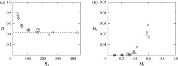
Figure 3(a) shows
 $D=\langle {\it\epsilon}\rangle L/u^{3}\langle {\it\rho}\rangle$
versus
 $R_{{\it\lambda}}$
from our database. Qualitatively, the figure is very similar to that in incompressible flows (Sreenivasan Reference Sreenivasan1984; Donzis et al.
Reference Donzis, Sreenivasan and Yeung2005). In particular, there is a decrease of
 $D$
with
 $R_{{\it\lambda}}$
for low values of
 $R_{{\it\lambda}}$
, but approaches an asymptotic value at high
 $R_{{\it\lambda}}$
. The asymptotic state appears to be reached at
 $R_{{\it\lambda}}\approx 100$
consistent with previous incompressible results (Sreenivasan Reference Sreenivasan1984; Donzis et al.
Reference Donzis, Sreenivasan and Yeung2005). For
 $M_{t}\approx 0.3$
, the asymptotic value of
 $D$
is around
 $0.43$
. For higher
 $M_{t}$
, the achievable
 $R_{{\it\lambda}}$
is not as high making it difficult to assess with certainty the value at the asymptotic state.
The phenomenological underpinning of dissipative anomaly is that large scales set the rate at which energy is transferred through increasingly smaller scales until viscosity is effective and dissipates this energy. A straightforward extension to compressible flows would indicate that
 $D$
approach a constant too at high
 $R_{{\it\lambda}}$
, which is approximately, what is seen in figure 3. However, in compressible flows, the mean dissipation could be decomposed into solenoidal and dilatational component, and hence, a similar asymptotic constant can be established for each (
 $D_{s},D_{d}$
). Thus, if dissipative anomaly holds, both components should approach an asymptotic state at high
 $R_{{\it\lambda}}$
. Since
 $D_{s}$
is just the difference between
 $D$
and
 $D_{d}$
, we show
 $D_{d}$
in figure 3(b) as a function of
 $M_{t}$
. Though the overall contribution from
 $D_{d}$
is less than 5 % for the cases considered, there is a dramatic increase in its relative contribution for
 $M_{t}>0.3$
. Thus, one can expect the asymptotic value of
 $D$
to depend on
 $M_{t}$
though it may be noticeable only at much higher
 $M_{t}$
. For the range of
 $M_{t}$
considered in this paper,
 $D$
is only weakly affected by compressibility. Simulations at increasingly higher Reynolds and Mach numbers are needed to reach an unambiguous conclusion about the dependence of the asymptotic constant on
 $M_{t}$
.
Variation of (a) normalized mean energy dissipation rate (
 $D$
), and (b) its dilatational component (
 $D_{d}$
) with
 $M_{t}$
. Symbols for different Mach numbers in (a) correspond to
 $M_{t}\approx 0.1$
(○),
 $0.2$
(▫),
 $0.3$
(▵),
 $0.4$
(♢), and
 $0.6$
(▿), and for different Reynolds numbers in (b) correspond to
 $R_{{\it\lambda}}\approx 38$
(○),
 $60$
(▫),
 $100$
(▵),
 $160$
(♢),
 $270$
(▿), and
 $450$
(◃).

4.2. Velocity and length scales
Kolmogorov (Reference Kolmogorov1941) defined characteristic scales for the smallest scales of motion. The well-known Kolmogorov length, velocity and time scales are, respectively,
 $$\begin{eqnarray}{\it\eta}\equiv ({\it\nu}^{3}/{\it\varepsilon})^{1/4},\quad u_{{\it\eta}}\equiv ({\it\nu}{\it\varepsilon})^{1/4},\quad {\it\tau}_{{\it\eta}}\equiv ({\it\nu}/{\it\varepsilon})^{1/2}.\end{eqnarray}$$
Since this applies to incompressible flows, the kinematic viscosity
 ${\it\nu}$
is constant (and thus brackets are omitted) and
 ${\it\varepsilon}$
is the mean energy dissipation rate per unit mass. These relations lead to a simple scaling law if the normalized mean energy dissipation rate asymptotes to a constant (
 ${\it\varepsilon}L/u^{3}=D$
, as shown in § 4.1). Substituting
 ${\it\varepsilon}\propto u^{3}/L$
in (4.2) and after some algebra, we obtain
 $$\begin{eqnarray}\frac{{\it\lambda}}{{\it\eta}}\sim R_{{\it\lambda}}^{1/2},\quad \frac{L}{{\it\eta}}\sim R_{{\it\lambda}}^{3/2},\quad \frac{u}{u_{{\it\eta}}}\sim R_{{\it\lambda}}^{1/2},\end{eqnarray}$$
where
 $L$
is the integral length scale.
Scaling of (a) Taylor micro scale (
 ${\it\lambda}$
) and integral length scale (
 $L$
) and (b) Kolmogorov velocity scale (
 $u_{{\it\eta}}$
). Dashed lines indicate classical Kolmogorov scaling for incompressible turbulence:
 ${\it\lambda}/{\it\eta}\sim R_{{\it\lambda}}^{1/2}$
,
 $L/{\it\eta}\sim R_{{\it\lambda}}^{3/2}$
,
 $u/u_{{\it\eta}}\sim R_{{\it\lambda}}^{1/2}$
. Symbols for different
 $M_{t}$
as in figure 3(a).

The extension of (4.2) to compressible flows, though typically straightforward, is not unique. Since
 ${\it\nu}$
varies in space and time, one could devise dimensionally consistent alternatives. For example, one could use
 $\langle {\it\mu}\rangle /\langle {\it\rho}\rangle$
or
 $\langle {\it\mu}/{\it\rho}\rangle$
. Similarly, the energy dissipation rate per unit mass in a compressible flow can be taken as
 $\langle {\it\epsilon}\rangle /\langle {\it\rho}\rangle$
or
 $\langle {\it\epsilon}/{\it\rho}\rangle$
. Indeed, one can find different definitions using these alternatives in the literature (Shivamoggi Reference Shivamoggi1995; Samtaney et al.
Reference Samtaney, Pullin and Kosovic2001; Wang et al.
Reference Wang, Shi, Wang, Xiao, He and Chen2011). Although we have found that, for the range of parameters studied here, there is no appreciable difference between the different forms, we prefer to proceed by extending Kolmogorov (Reference Kolmogorov1941) reasoning to compressible flows. If we assert that small scales are independent of large scales and will only depend on the rate at which kinetic energy is converted into heat
 $\langle {\it\epsilon}\rangle$
, the mean viscosity
 $\langle {\it\mu}\rangle$
and the mean density
 $\langle {\it\rho}\rangle$
, then dimensional analysis yields:
 $$\begin{eqnarray}{\it\eta}\equiv (\langle {\it\mu}\rangle ^{3}/\langle {\it\epsilon}\rangle \langle {\it\rho}\rangle ^{2})^{1/4},\quad u_{{\it\eta}}\equiv (\langle {\it\mu}\rangle \langle {\it\epsilon}\rangle /\langle {\it\rho}\rangle ^{2})^{1/4},\quad {\it\tau}_{{\it\eta}}\equiv (\langle {\it\mu}\rangle /\langle {\it\epsilon}\rangle )^{1/2}.\end{eqnarray}$$
With these definitions and
 $\langle {\it\epsilon}\rangle \propto \langle {\it\rho}\rangle u^{3}/L$
, we obtain again (4.3).
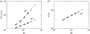
In figure 4(a) we plot the non-dimensionalized Taylor micro-scales and integral length scale. While the scaling of Taylor micro-scales conform very well to that of the proposed scaling (
 ${\it\lambda}/{\it\eta}\sim R_{{\it\lambda}}^{1/2}$
) without any
 $M_{t}$
dependence, the scaling of integral length scales deviate slightly from
 $R_{{\it\lambda}}^{3/2}$
at low Reynolds number. This is not surprising given that Kolmogorov scaling has been proposed only when the Reynolds number is high enough. However, even at high Reynolds numbers, a close inspection of the data seems to suggest a slight correction with the data presenting a shallower power law. Results at higher Reynolds numbers are needed to unambiguously determine this departure. In any case, for turbulent Mach numbers up to 0.6, the effect of compressibility on low order quantities tend to be weak as is also seen in figure 4(b) for Kolmogorov velocity scale.
5. Equipartition of energy in homogeneous compressible turbulence
The phenomenon of equipartition is often associated with non-dissipative linear waves where the sum of potential and kinetic energy is constant. But in turbulence, where nonlinear as well as dissipative effects are observed at any Reynolds number, such distribution of energy, in principle, cannot a priori be justified. However, Kraichnan (Reference Kraichnan1955) observed that for an adiabatically compressible fluid at low Mach numbers, the vorticity and acoustic modes are coupled by the nonlinear terms and drive the system to an equilibrium state. Similarly, Sarkar et al. (Reference Sarkar, Erlebacher, Hussaini and Kreiss1991) decomposed the Navier–Stokes equations into compressible and incompressible parts and suggested equipartition at low
 $M_{t}$
for the compressible component.
The concept of acoustic equilibrium could be interpreted in strong or weak forms. In the former, the equilibrium between dilatational components of pressure and velocity is established for all wavenumbers, while in the latter they are expected to be valid only in a global average sense (Sagaut & Cambon Reference Sagaut and Cambon2008). The equipartition functions
 $F_{w}$
and
 $F_{s}$
for weak and strong forms respectively are then (Hamba Reference Hamba1999; Sarkar et al.
Reference Sarkar, Erlebacher, Hussaini and Kreiss1991),
 $$\begin{eqnarray}\displaystyle & \displaystyle F_{w}\langle p^{d}p^{d}\rangle ={\it\gamma}^{2}M_{t}^{2}{\it\chi}\langle p\rangle ^{2}, & \displaystyle\end{eqnarray}$$
 $$\begin{eqnarray}\displaystyle & \displaystyle F_{s}E_{p^{d}}=\langle {\it\rho}\rangle ^{2}\langle c\rangle ^{2}E_{u^{d}}. & \displaystyle\end{eqnarray}$$
 $E_{p^{d}}$
and
 $E_{u^{d}}$
are the spectra of dilatational pressure and velocity respectively, and
 ${\it\chi}=\langle \mathscr{K}^{d}\rangle /\langle \mathscr{K}\rangle$
is the fraction of mean dilatational kinetic energy to the mean kinetic energy in the system. For perfect equipartition, one expects
 $F_{s}=F_{w}=1$
.
The equipartition of energy in the weak sense, though theoretically derived for the low-Mach number subsonic regime, has found support at
 $M_{t}$
as high as
 $0.5$
in DNS of decaying turbulence (Sarkar et al.
Reference Sarkar, Erlebacher, Hussaini and Kreiss1991). In these flows, the initial transient are thought to be dominated by acoustics. Viscous and convective effects are expected to play a larger role at later times. In stationary flows with external forcing, on the other hand, it is difficult to associate a physical time at which each of these processes dominate independently. It is likely that both the acoustic and turbulent phenomena occur concurrently at different time scales based on the Mach number. At higher levels of compressibility, the coupling between the acoustic and vorticity modes is also enhanced and could possibly distort the equipartition. In general, the existing literature lends support to equipartition only in the low-Reynolds low-Mach number limit (see e.g. Kida & Orszag Reference Kida and Orszag1990; Miura & Kida Reference Miura and Kida1995). Due to its widespread application and usefulness in turbulence modelling, we now investigate the validity of equipartition with emphasis on its
 $M_{t}$
scaling.
Equipartition in the weak and strong sense. (a) Variation of equipartition function
 $F_{w}$
for different
 $M_{t}$
according to the weak-equilibrium hypothesis. Dashed line indicates
 $F_{w}=1$
. (b) Spectra of dilatational components of pressure
 $E_{p_{d}}(k)$
(grey) and velocity
 $\langle {\it\rho}\rangle ^{2}\langle c\rangle ^{2}E_{\boldsymbol{u}^{\boldsymbol{d}}}(k)$
(black) at
 $M_{t}\approx$
 $0.1$
(dash-dotted),
 $0.3$
(dash),
 $0.6$
(solid).

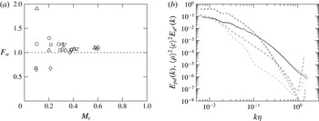
Figure 5(a) shows the variation of the ensemble-averaged equipartition function
 $F_{w}$
with
 $M_{t}$
. For
 $M_{t}<0.3$
, the data is scattered around
 $F_{w}\approx 1$
, with significant Reynolds number dependence. Beyond
 $M_{t}\approx 0.3$
,
 $F_{w}$
is much closer to unity with weak
 $R_{{\it\lambda}}$
effects. The scatter in the data may be directly related to the scaling of normalized dilatational pressure (
 $\langle p^{d}p^{d}\rangle ^{1/2}/\langle p\rangle \approx M_{t}^{2}$
) which is discussed in § 6. As will be shown in that section, while at high
 $M_{t}$
the data conforms to this scaling, at low
 $M_{t}$
there is considerable deviation. This seems to indicate the existence of a difference between decaying and forced turbulence. In decaying flows, during the acoustic transient period, dilatational pressure plays a crucial role in bringing the system towards equipartition (Sarkar et al.
Reference Sarkar, Erlebacher, Hussaini and Kreiss1991). As we will show in § 6, the role of dilatational pressure in forced flows is not dominant unless
 $M_{t}$
increases beyond a threshold.
Miura & Kida (Reference Miura and Kida1995) observed
 $F_{w}$
to be slightly in excess of unity (
 $F_{w}\approx 1.15$
) in their simulations of forced compressible turbulence at
 $R_{{\it\lambda}}\approx 35$
and
 $M_{t}\approx 0.14$
. In our simulations as well,
 $F_{w}$
is slightly greater than unity. This small difference between the current DNS and the theoretical value of unity from Sarkar et al. (Reference Sarkar, Erlebacher, Hussaini and Kreiss1991) may not be unexpected if one recalls their assumptions. First, the theory assumes isentropic fluctuations which is not strictly correct (Donzis & Jagannathan Reference Donzis and Jagannathan2013a
). Second, the decomposition of the velocity field does not correspond to the Helmholtz decomposition as the one used here. While still not strictly equal to unity, our DNS data support an approximate balance between the dilatational motions and pressure.
In real flows, one may be more interested in the total pressure instead of its solenoidal or dilatational component in which case one can recast the non-dimensional parameter,
 $F_{w}$
, in terms of total pressure. It has been argued (Sarkar et al.
Reference Sarkar, Erlebacher, Hussaini and Kreiss1991; Sagaut & Cambon Reference Sagaut and Cambon2008) that this would lead to
 $F_{T}=\langle \mathscr{K}^{d}\rangle {\it\gamma}\langle p\rangle \langle {\it\rho}\rangle /\langle {p^{\prime }}^{2}\rangle$
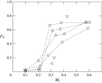
. In figure 6, we show
 $F_{T}$
which would approach unity if equipartition is achieved. While lower values of
 $M_{t}$
are necessary to be more conclusive, the data suggest an asymptotic state at very low
 $M_{t}$
when the ratio is close to zero with a weak Reynolds-number effect. We note that this is in contrast with decaying sheared flows starting from purely solenoidal fields (Bertsch et al.
Reference Bertsch, Suman and Girimaji2012). This may again be due to the differing role of dilatational pressure in both forced and decaying flows. Around
 $M_{t}\approx 0.3$
, there is a sharp increase in
 $F_{T}$
followed by a plateau at
 $M_{t}\approx 0.6$
with the value of
 $F_{T}$
around
 $0.70$
. This transition in flow statistics at
 $M_{t}\approx 0.3$
was also observed in figure 3(b).
Equipartition function
 $F_{w}$
recast into
 $F_{T}$
using the weak equilibrium hypothesis. Symbols for different Reynolds numbers as in figure 3(b).

In general the weak form of equipartition does not imply the strong form. In particular, since
 $F_{w}$
is based on r.m.s. quantities, most of its contribution comes from large scales. The strong form, on the other hand, considers scale-by-scale equipartition based on the spectral content of dilatational velocity and pressure. In figure 5(b) we show the spectra
 $E_{p^{d}}$
and
 $E_{u^{d}}$
(normalized by
 $\langle {\it\rho}\rangle ^{2}\langle c\rangle ^{2}$
) for different
 $M_{t}$
at
 $R_{{\it\lambda}}\approx 160$
. At low
 $M_{t}$
, the spectral content of dilatational pressure is smaller than that of the dilatational velocity at all scales, with a stronger effect at high wavenumbers. Beyond the threshold
 $M_{t}\approx 0.3$
,
 $E_{p^{d}}$
and
 $\langle {\it\rho}\rangle ^{2}\langle c\rangle ^{2}E_{u^{d}}$
begin to overlap over an increasingly wider range of scales. At
 $M_{t}\approx 0.6$
the two spectra almost collapse at all wavenumbers. While the effect of forcing may be in the large scales either to help or distort equipartition, its effect on small scales is expected to be weaker as the Reynolds number is increased. Thus, the data suggest that at high Reynolds numbers and Mach numbers beyond
 $M_{t}\approx 0.3$
, the strong acoustic equilibrium hypothesis is approximately valid for stationary flows. We note that these conclusions are for scales larger than Kolmogorov scale, and are thus unaffected by the well-known (Watanabe & Gotoh Reference Watanabe and Gotoh2007; Ishihara et al.
Reference Ishihara, Gotoh and Kaneda2009) residual errors at very high wavenumbers (
 $k{\it\eta}>1$
). We also note that at the largest scales, the creation of dilatational motions may be related to the stochastic nature of the forcing. For example, one may expect that the random changes in direction of large-scale structures, though slow for this type of forcing, may generate pressure waves associated with dilatational motions. Thus, just as in incompressible flows, there is no expectation of a universal behaviour at the large scales.
In summary, for forced stationary flows, the weak form of the equipartition function
 $F_{w}$
tends to unity at high
 $M_{t}$
.
 $F_{T}$
, on the other hand, does not approach unity (though it is not too far from it) indicating a non-negligible contribution from solenoidal pressure even at high
 $M_{t}$
. The (strong) equipartition function
 $F_{s}$
, is seen to be valid also at high
 $M_{t}$
in stationary flows. We emphasize that the dilatational motions present in the flow are the result of the dynamics of the Navier–Stokes equations and not imposed externally in the form of initial conditions, boundary conditions or nature of the forcing.
5.1. Consequences of equipartition: scaling of dilatational components
One of the results from the asymptotic analysis of Erlebacher et al. (Reference Erlebacher, Hussaini, Kreiss and Sarkar1990) and Sarkar et al. (Reference Sarkar, Erlebacher, Hussaini and Kreiss1991) is the model for the dilatational dissipation rate in the low Mach-number regime (
 $\langle {\it\epsilon}^{d}\rangle \propto M_{t}^{2}\langle {\it\epsilon}^{s}\rangle$
). This result was derived by assuming equipartition in the form
 $F_{w}\approx 1$
. In addition, this model assumed the ratio of solenoidal and dilatational Taylor scales to be a constant, which as we show below, follows a power law in
 $M_{t}$
instead. Note that based on the definition of Taylor scales and assuming that density is weakly correlated with the velocity field, we can show that the ratio of solenoidal to dilatational Taylor scales varies as,
 ${\it\lambda}^{s}/{\it\lambda}^{d}\sim \sqrt{(\langle \mathscr{K}^{s}\rangle /\langle \mathscr{K}^{d}\rangle )(\langle {\it\epsilon}^{d}\rangle /\langle {\it\epsilon}^{s}\rangle )}$
. It can be clearly seen that this would become independent of Reynolds and Mach number only if
 $\langle \mathscr{K}^{d}\rangle /\langle \mathscr{K}^{s}\rangle$
and
 $\langle {\it\epsilon}^{d}\rangle /\langle {\it\epsilon}^{s}\rangle$
scale similarly. As will be shown momentarily, they scale differently and a correction factor has to be incorporated while modelling
 ${\it\lambda}^{s}/{\it\lambda}^{d}$
.
Available results on the scaling of dissipation appear not to be in agreement with each other. Bertoglio, Bataille & Marion (Reference Bertoglio, Bataille and Marion2001) suggested that
 $\langle {\it\epsilon}^{d}\rangle /\langle {\it\epsilon}^{s}\rangle$
also scales as
 $M_{t}^{2}$
based on an EDQNM analysis at low Mach numbers. Ristorcelli (Reference Ristorcelli1997) and Fauchet & Bertoglio (Reference Fauchet, Bertoglio and Frisch1998), on the other hand, proposed
 $M_{t}^{4}$
. It is worth noting here that the scaling exponents predicted by Erlebacher et al. (Reference Erlebacher, Hussaini, Kreiss and Sarkar1990) and Ristorcelli (Reference Ristorcelli1997) are based on different assumptions. While the former decomposed the compressible problem based on convective and acoustic time scales, the latter assumed that the length scales (inner and outer scales) are disparate. However, both these analyses were made for low
 $M_{t}$
. An even steeper dependence, as
 $M_{t}^{5}$
, at high turbulent Mach numbers has also been proposed using EDQNM (Sagaut & Cambon Reference Sagaut and Cambon2008). Other relations have also been put forth in the literature as
 $\langle {\it\epsilon}^{d}\rangle \propto \langle {\it\epsilon}^{s}\rangle F(M_{t})$
, where different relations are possible based on the definition of
 $F(M_{t})$
(Zeman Reference Zeman1990; Blaisdell & Zeman Reference Blaisdell, Zeman and Spinks1992). Some of these results have been supported by simulations of decaying compressible turbulence at low
 $R_{{\it\lambda}}$
and
 $M_{t}$
though conclusions may be dependent on specific features of the particular initial conditions used (Vreman, Sandham & Luo Reference Vreman, Sandham and Luo1996; Ristorcelli Reference Ristorcelli1997). One way of removing the dependence on initial condition is to force the simulation by adding energy to the large scales so that a statistically stationary state is achieved. This is the case in the present study.
Ratio of dilatational to solenoidal (a) dissipation (b) turbulent kinetic energy. Symbols for different Reynolds numbers as in figure 3(b). Solid line in (a) corresponds to best-fit curve
 $M_{t}^{4.1}$
and dash-dotted line in (b) corresponds to a representative
 $M_{t}^{2}$
and
 $M_{t}^{4}$
curve.

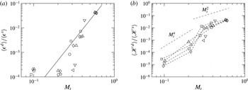
Consider first the ratio of solenoidal to dilatational dissipation in figure 7. The DNS appears to suggest two different scaling ranges depending on
 $M_{t}$
with the transition occurring around
 $M_{t}\approx 0.3$
. While the contribution of dilatational dissipation is negligibly small at low
 $M_{t}$
, it increases sharply beyond
 $M_{t}\geqslant 0.3$
, following a steep power law,
 $\langle {\it\epsilon}^{d}\rangle /\langle {\it\epsilon}^{s}\rangle \sim M_{t}^{4.1}$
for the range of
 $M_{t}$
investigated. This indicates that the contribution of dilatational motions to dissipation grows quickly as
 $M_{t}$
increases, as has been noted in figure 3(b). Stronger fluctuations of local values of dilatational dissipation at high
 $M_{t}$
may also indicate stronger intermittency, a phenomenon with important implications in shock-turbulence interactions (Donzis & Jagannathan Reference Donzis and Jagannathan2013b
). The Reynolds number effect on the ratio of the different components of dissipation is seen to be very weak.
Scaling laws for the ratio of dilatational and solenoidal kinetic energy,
 $\langle \mathscr{K}^{d}\rangle /\langle \mathscr{K}^{s}\rangle$
, have also been proposed in the literature. For example, Sarkar et al. (Reference Sarkar, Erlebacher, Hussaini and Kreiss1991) suggested a
 $M_{t}^{2}$
dependence at low
 $M_{t}$
based on an asymptotic analysis while Fauchet & Bertoglio (Reference Fauchet, Bertoglio and Frisch1998) proposed
 $M_{t}^{4}$
and
 $M_{t}^{2}\mathit{Re}_{L}$
scaling using an EDQNM approximation with different decorrelation functions where
 $\mathit{Re}_{L}$
is the integral scale Reynolds number. Figure 7(b) shows this ratio from our DNS database. Similar to the scaling of ratio of dissipation rates, we can distinguish different scaling regimes at low and high
 $M_{t}$
that vary as
 $M_{t}^{4}$
and
 $M_{t}^{2}$
respectively. Their dependence on Reynolds number becomes weak at high
 $M_{t}$
.
We can now use the scaling of dissipation and kinetic energy to obtain the ratio of Taylor scales. Since both
 $\langle {\it\epsilon}^{d}\rangle /\langle {\it\epsilon}^{s}\rangle$
and
 $\langle \mathscr{K}^{d}\rangle /\langle \mathscr{K}^{s}\rangle$
appear to be independent of
 $R_{{\it\lambda}}$
for
 $M_{t}\geqslant 0.3$
, the ratio of solenoidal and dilatational Taylor scales should also be independent of
 $R_{{\it\lambda}}$
at high
 $M_{t}$
. Using the best fits for
 $\langle {\it\epsilon}^{d}\rangle /\langle {\it\epsilon}^{s}\rangle$
and
 $\langle \mathscr{K}^{d}\rangle /\langle \mathscr{K}^{s}\rangle$
at high
 $M_{t}$
, we obtain
 ${\it\lambda}^{s}/{\it\lambda}^{d}\sim \sqrt{M_{t}^{4.1}/M_{t}^{2.2}}\sim M_{t}^{0.9}$
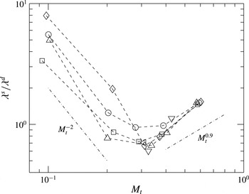
. This result, along with DNS data is shown in figure 8. Again, two qualitatively different regimes can be identified with a transition around
 $M_{t}\approx 0.3$
. For low Mach numbers we see a strong Reynolds number dependence and a decreasing trend with
 $M_{t}$
. This is due to the Reynolds number dependence seen at low
 $M_{t}$
in the scaling of
 $\langle \mathscr{K}^{d}\rangle /\langle \mathscr{K}^{s}\rangle$
. This dependence weakens beyond
 $M_{t}\approx 0.3$
eventually becoming almost independent of
 $R_{{\it\lambda}}$
at
 $M_{t}\approx 0.6$
. A best-fit power-law for
 $M_{t}\geqslant 0.3$
shows a
 $M_{t}^{1.2}$
scaling which is close to the prediction.
Ratio of solenoidal and dilatational Taylor scales. Symbols for different Reynolds numbers as in figure 3(b). Dash-dotted lines correspond to a representative
 $M_{t}^{-2}$
and
 $M_{t}^{0.9}$
.

From figure 8 we conclude that the DNS data do not support a constant
 ${\it\lambda}^{s}/{\it\lambda}^{d}$
as assumed by Sarkar et al. (Reference Sarkar, Erlebacher, Hussaini and Kreiss1991). However, the latter considered only decaying flows and, thus, does not account for the effect of forcing. As we have already shown above, statistically steady forced flows present significant differences, for example in equilibrium states (equipartition), compared to decaying flows.
6. Pressure statistics
6.1. Solenoidal and dilatational pressure scaling
Considering that equipartition appears to depend on
 $R_{{\it\lambda}}$
and
 $M_{t}$
, it seems important to understand not only total pressure, but in particular the solenoidal and dilatational components as mentioned in § 3.3. Though different decompositions are possible (Sarkar Reference Sarkar1992), (3.9) is widely used in turbulence modelling. Since by definition the solenoidal pressure satisfies the incompressible pressure Poisson equation, we can expect the relation,
 $p_{rms}^{s}\sim \langle {\it\rho}\rangle \boldsymbol{u}_{rms}^{\boldsymbol{s}}\boldsymbol{u}_{rms}^{\boldsymbol{s}}$
, to be only weakly affected by Mach number effects (Erlebacher et al.
Reference Erlebacher, Hussaini, Kreiss and Sarkar1990).
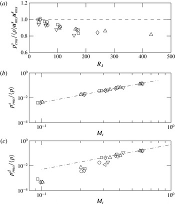
Figure 9(a) shows that indeed
 $p_{rms}^{s}$
scales as
 $\langle {\it\rho}\rangle \langle \boldsymbol{u}_{i}^{\boldsymbol{s}}\boldsymbol{u}_{i}^{\boldsymbol{s}}\rangle$
with a weak Mach number dependence. For
 $M_{t}\approx 0.1$
the high Reynolds number asymptotic constant is around 0.88 close to the incompressible case at 0.91 (Donzis, Sreenivasan & Yeung Reference Donzis, Sreenivasan and Yeung2012). However, at the highest Reynolds number available for
 $M_{t}\approx 0.3$
(
 $R_{{\it\lambda}}\approx 450$
), the asymptotic constant decreases to around
 $0.82$
. While clearly data at higher Reynolds number are needed to establish asymptotes conclusively, small trends with Mach number appear to be present.
One could extend the incompressible scaling to total pressure fluctuations,
 $p_{rms}\sim \langle {\it\rho}\rangle u^{2}$
, and normalize by the mean pressure to obtain
 $p_{rms}/\langle p\rangle \sim \langle {\it\rho}\rangle u^{2}/\langle {\it\rho}\rangle R\langle T\rangle \sim u^{2}/c^{2}\sim M_{t}^{2}$
. Recent numerical simulations suggest that
 $p_{rms}/\langle p\rangle$
grows slightly faster with
 $M_{t}$
, as
 $M_{t}^{2.2}$
(Donzis & Jagannathan Reference Donzis and Jagannathan2013a
). This departure can be ascertained by exploring the scaling of the individual components of pressure. When
 $p_{rms}^{s}$
is scaled by the mean pressure, as shown in figure 9(b), we see excellent agreement with
 $M_{t}^{2}$
and almost no Reynolds number dependence. However, when the dilatational pressure is scaled similarly (in figure 9(c)), a steeper exponent is observed at low
 $M_{t}$
(close to 4.0) while an emerging
 $M_{t}^{2}$
scaling is seen for
 $M_{t}\geqslant 0.3$
. The higher exponent at low
 $M_{t}$
may explain the minor deviation seen in Donzis & Jagannathan (Reference Donzis and Jagannathan2013a
) only if dilatational pressure provides a non-negligible contribution to total pressure at low
 $M_{t}$
. As we show momentarily, however, this is not the case.
Scaling of solenoidal pressure (a,b) and dilatational pressure (c). Symbols for different Mach numbers in (a) and Reynolds numbers in (b,c) as in figure 3. Dashed line in (a) corresponds to
 $p_{rms}^{s}/\langle {\it\rho}\rangle \boldsymbol{u}_{\mathit{rms}}^{\boldsymbol{s}}\boldsymbol{u}_{\mathit{rms}}^{\boldsymbol{s}}=1$
for reference. Dash-dotted lines in (b,c) indicate a slope of 2.

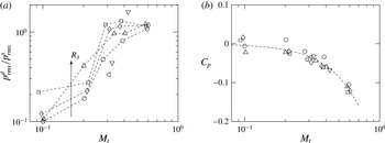
In order to assess the relative contributions of the dilatational and solenoidal pressure, the ratio of their r.m.s. values is shown in figure 10(a). While at low
 $M_{t}$
,
 $p_{rms}^{d}$
is only approximately 10 % of
 $p_{rms}^{s}$
, there is a sharp increase around
 $M_{t}\approx 0.3$
. Beyond
 $M_{t}\approx 0.3$
, the ratio remains close to
 $1.0$
, with a weaker Reynolds number dependence than at lower
 $M_{t}$
. Here, we note again the qualitative change in behaviour seen at
 $M_{t}\approx 0.3$
.
(a) Ratio of dilatation to solenoidal pressure fluctuations. (b) Correlation coefficient,
 $C_{p}$
between solenoidal and dilatational pressure respectively. Dashed line indicates a best-fit curve,
 $C_{p}=-0.334M_{t}^{2}$
. Symbols for different Reynolds numbers as in figure 3(b).

While a linear analysis of the (inviscid) governing equation may suggest some independence between the components of pressure, it is expected that in real flows, solenoidal and dilatational pressure may in fact be correlated to a degree that would depend on the Reynolds and Mach numbers. Note that this is different from the velocity field whose solenoidal and dilatational components are by construction uncorrelated. The correlation coefficient for pressure components from the DNS data is plotted in figure 10(b). While at low Mach numbers the solenoidal and dilatational pressure behave independently, at higher Mach numbers they become more negatively correlated. One can also see a decreasing dependence on Reynolds number as
 $M_{t}$
increases. If by lack of any theoretical guidance, one assumes a power-law scaling in
 $M_{t}$
, the data is seen to be consistent with
 $C_{p}=-0.334M_{t}^{2}$
. Since by construction, correlation coefficients can take values in the interval
 $[-1,1]$
, this expression is clearly inadequate for higher
 $M_{t}$
.
From a theoretical perspective, one could now argue that this particular decomposition of
 $p$
has merit only at low
 $M_{t}$
where the two components are uncorrelated, just like the Helmholtz decomposition for the velocity field. At high
 $M_{t}$
, on the other hand, as dilatational pressure becomes more correlated with solenoidal pressure, its ability to isolate compressibility effects seems to weaken. Yet, from a practical perspective, this correlation might be useful for turbulence modelling. As we have seen, solenoidal pressure is virtually unaffected by compressibility for the range of Reynolds and Mach numbers investigated. This suggests that the p.d.f. of
 $p^{s}$
may be modelled according to theories from incompressible turbulence and dilatational pressure obtained from this model. For instance, in incompressible turbulence, Vedula & Yeung (Reference Vedula and Yeung1999) proposed a stretched exponential fit for the negative tails of pressure, and a Gaussian distribution for positive tails. Using the correlation between solenoidal and dilatational pressure it is possible to model both components of pressure, and thus the total pressure fluctuations.
We can now go back to the departures from
 $M_{t}^{2}$
observed for total pressure fluctuations in Donzis & Jagannathan (Reference Donzis and Jagannathan2013a
). By considering both figures 9, and 10 together we can see that at low
 $M_{t}$
, where the
 $M_{t}$
dependence is stronger for dilatational pressure, its contribution to total pressure is small. However, as
 $M_{t}$
increases dilatational pressure provides an increasingly large contribution. By using
 $p^{\prime }=p^{s}+p^{d}$
we can easily obtain
 $\langle p^{\prime 2}\rangle =\langle p^{s}p^{s}\rangle +\langle p^{d}p^{d}\rangle +2\langle p^{s}p^{d}\rangle$
or
 $$\begin{eqnarray}\frac{\langle {p^{\prime }}^{2}\rangle }{\langle p\rangle ^{2}}=\frac{\langle (p^{s})^{2}\rangle }{\langle p\rangle ^{2}}+\frac{\langle (p^{d})^{2}\rangle }{\langle p\rangle ^{2}}+2C_{p}\frac{\langle (p^{s})^{2}\rangle ^{1/2}}{\langle p\rangle }\frac{\langle (p^{d})^{2}\rangle ^{1/2}}{\langle p\rangle }.\end{eqnarray}$$
Using figures 9(a) and 10(b), we can see that the first term on the right-hand side scales as
 $M_{t}^{4}$
which is expected to be the dominant term at low Mach numbers. In the other limit, at high
 $M_{t}$
, the variance of dilatational pressure also scales as
 $M_{t}^{4}$
and since
 $C_{p}$
cannot continue to grow with
 $M_{t}$
due to its boundedness, it is plausible to assume that it will approach a constant. In this case, the last term on the right-hand side will also scale as
 $M_{t}^{4}$
. Thus,
 $\langle p^{\prime 2}\rangle$
will scale as
 $M_{t}^{4}$
at low and high
 $M_{t}$
but the prefactors at both limits may be different.
Therefore, we conclude that the apparent departure from
 $M_{t}^{4}$
scaling for the variance of pressure when considering the entire range of
 $M_{t}$
in Donzis & Jagannathan (Reference Donzis and Jagannathan2013a
) appears to reflect the transition of dilatational pressure from low to high Mach numbers at
 $M_{t}\approx 0.3$
.
6.2. P.d.f. of pressure
Large pressure fluctuations or asymmetries in these fluctuations cannot be captured by its first or second-order moments. Instead one needs to study high-order moments or even the entire p.d.f. The skewness of pressure
 $S_{p}=\langle p^{\prime 3}\rangle /\langle p^{\prime 2}\rangle ^{3/2}$
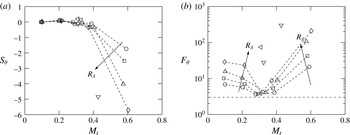
, for example, which measures the asymmetry of the p.d.f., has been shown to change from negative to positive as
 $M_{t}$
is increased (Donzis & Jagannathan Reference Donzis and Jagannathan2013a
). This transition occurs around
 $M_{t}\approx 0.3$
, similar to other flow statistics presented in previous sections. Negative and positive skewness represents an increased likelihood of moderately low and high-pressure regions in the flow respectively and indicates a qualitative difference in the role of pressure at low and high
 $M_{t}$
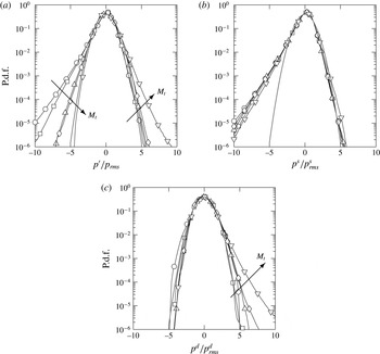
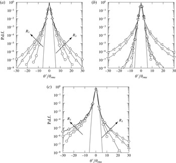
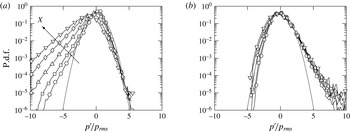
. In figure 11(a) we show this change in the p.d.f. of pressure at
 $R_{{\it\lambda}}\approx 160$
for different
 $M_{t}$
.
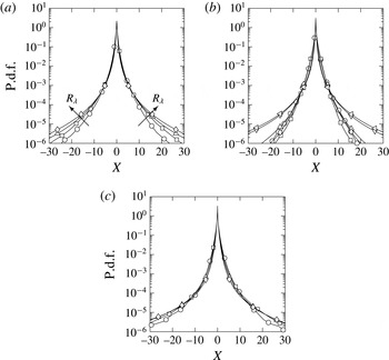
P.d.f. of (a) pressure fluctuations and its (b) solenoidal and (c) dilatational components at
 $R_{{\it\lambda}}\approx 160$
for different
 $M_{t}$
. Lines in grey correspond to a Gaussian distribution. Symbols for different Mach numbers as in figure 3(a). Arrows are in the direction of increasing
 $M_{t}$
.

It has been suggested (Blaisdell et al.
Reference Blaisdell, Mansour and Reynolds1993) that this change is a result of pressure being a positive quantity and therefore bounded from the negative side (
 $p^{\prime }>-\langle p\rangle$
). However, this does not provide a mechanism that can explain why or how pressure fluctuations increase on the positive side. One could explore the p.d.f. of solenoidal and dilatational pressure individually, for example, to elucidate the contribution from each component.
The p.d.f. of
 $p^{s}$
(
 $f_{ps}$
) shown in figure 11(b), has a negligible dependence on
 $M_{t}$
and remains negatively skewed for the range of
 $M_{t}$
investigated, with positive fluctuations following a Gaussian distribution. This is consistent with results in incompressible turbulence (Pumir Reference Pumir1994; Vedula & Yeung Reference Vedula and Yeung1999). On the other hand, the p.d.f. of
 $p^{d}$
(
 $f_{pd}$
), shown in figure 11(c), remains close to Gaussian for negative fluctuations, but becomes positively skewed beyond
 $M_{t}\approx 0.3$
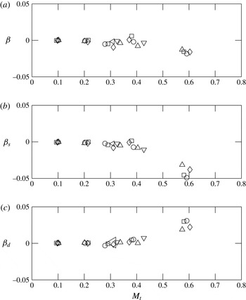
. Thus the positive skewness of pressure at high
 $M_{t}$
appears to be a direct result of the large contributions of dilatational pressure. Note that the appearance of dilatational pressure is a consequence of Navier–Stokes dynamics as the forcing scheme provides only solenoidal modes.
This conclusion is strengthened if we consider the following observations. First, since
 $p^{d}$
becomes anti-correlated with
 $p^{s}$
at high
 $M_{t}$
(see figure 10
b) and
 $f_{ps}$
is skewed to the left, we can expect the tails of
 $f_{pd}$
to be wider on the right. As long as this anti-correlation becomes stronger with
 $M_{t}$
and
 $p^{s}$
remains skewed to the left,
 $p^{d}$
would continue to show stronger and stronger positive fluctuations mirroring more and more the negative tails of solenoidal pressure. Second, in figure 10(a), we already observed that as
 $M_{t}$
is increased beyond
 $0.3$
, the dilatational pressure fluctuations tend to be of the same order as that of its solenoidal counterpart which suggests that strong positive fluctuations are related to dilatational effects. It then seems natural to investigate the differences in regions of low and high dilatational motions. This is the focus of the next sections.
6.3. P.d.f. of dilatation
The behaviour of dilatation is particularly relevant in understanding the effects of compressions and expansions in the flow. Though somewhat arbitrary, shocklets are commonly defined as regions with instantaneous dilatation being less than a threshold,
 ${\it\theta}^{\prime }<-3{\it\theta}_{rms}$
(Samtaney et al.
Reference Samtaney, Pullin and Kosovic2001) and have been suggested to have different effects on the flow. For instance, shocklets can increase the rate of dilatational dissipation. While considerable attention has been given to the role of shocklets, the effect of expansions has not been investigated in any detail. A strong local expansion, for instance, can result in a large value of pressure-dilatation correlation, which could bring about a strong energy transfer between kinetic and internal energy.
P.d.f. of dilatation at
 $M_{t}\approx$
(a) 0.1 (b) 0.3 (c) 0.6. Symbols for different Reynolds numbers as in figure 3. Arrows are in the direction of increasing
 $R_{{\it\lambda}}$
.

We consider the Reynolds and Mach number variation of the p.d.f. of normalized dilatation (
 ${\it\theta}^{\prime }/{\it\theta}_{rms}$
) for
 $M_{t}\approx 0.1,0.3,0.6$
in figure 12. At low
 $M_{t}$
, the tails of the p.d.f. become wider with
 $R_{{\it\lambda}}$
, but remains symmetric, indicating that regions of large positive and negative dilatation are equally likely to appear intermittently. This
 $R_{{\it\lambda}}$
effect is typical of all velocity gradients in incompressible turbulence (Donzis et al.
Reference Donzis, Yeung and Sreenivasan2008b
). A similar behaviour is observed at
 $M_{t}\approx 0.3$
, though tails appear to be narrower at low
 $R_{{\it\lambda}}$
. It is conceivable that this decline in the appearance of large gradients in the flow is related to the change in several flow statistics at
 $M_{t}\approx 0.3$
that has been investigated so far. For higher
 $R_{{\it\lambda}}$
, the tails grow wider but retain the symmetry. Since high
 $R_{{\it\lambda}}$
simulations are available only for
 $M_{t}\approx 0.3$
and
 $0.4$
, it is not possible to comment on their Mach number variation. Finally, at
 $M_{t}\approx 0.6$
, the p.d.f. becomes asymmetric with wider tails on the left, that grow with
 $R_{{\it\lambda}}$
.
More quantitative information about large fluctuations can be obtained by computing high-order moments, in particular skewness,
 $S_{{\it\theta}}$
, and flatness factors,
 $F_{{\it\theta}}=\langle {\it\theta}^{\prime 4}\rangle /\langle {\it\theta}^{\prime 2}\rangle ^{2}$
, which quantifies the asymmetry and the wideness of the tails. The variation of skewness and flatness of dilatation with
 $M_{t}$
is seen in figure 13(a,b). Beyond
 $M_{t}\approx 0.3$
, the negative skewness increases (in magnitude) with
 $M_{t}$
, a result also reported in the literature (Lee et al.
Reference Lee, Lele and Moin1991; Pirozzoli & Grasso Reference Pirozzoli and Grasso2004; Wang et al.
Reference Wang, Shi, Wang, Xiao, He and Chen2012).
Variation of (a) skewness and (b) flatness of dilatation with
 $M_{t}$
. Arrows are in the direction of increasing
 $R_{{\it\lambda}}$
. Symbols for different Reynolds number as in figure 3. Dash-dotted line in (b) corresponds to a flatness value of 3 for a Gaussian distribution. Dashed lines in (a,b) connect data at fixed Reynolds number for clarity except for the highest Reynolds numbers where not enough data at different
 $M_{t}$
are available to see trends (cf. table 1).

Percentage volume of normalized dilatation (
 ${\it\theta}^{\prime }/{\it\theta}_{rms}$
) in different bins.

While the
 $R_{{\it\lambda}}$
dependence of skewness is negligible at low
 $M_{t}$
, there is a substantial change with
 $M_{t}$
beyond
 $M_{t}\approx 0.3{-}0.4$
. The flatness values, on the other hand, show a decrease with
 $M_{t}$
until
 $M_{t}\approx 0.3{-}0.4$
when it reaches a value around
 $3.0$
(Gaussian) for
 $R_{{\it\lambda}}\lesssim 160$
, and then increase sharply. This behaviour is consistent with the narrowing of the p.d.f. at intermediate
 $M_{t}$
and at low
 $R_{{\it\lambda}}$
. The data at higher Reynolds numbers (
 $R_{{\it\lambda}}\approx 275,450$
) appear to have higher flatness value at
 $M_{t}\approx 0.3$
which may indicate stronger intermittency as
 $R_{{\it\lambda}}$
increases consistent with velocity gradients in incompressible flows. In order to assess the precise Reynolds and Mach number scaling of high order statistics, however, simulations at higher
 $R_{{\it\lambda}}$
and
 $M_{t}$
areneeded.
Large flatness value such as seen in figure 13, typically indicates that regions of large positive and negative dilatation appear intermittently in the flow. The percentage volume of their occurrence is given in table 2. While regions of strong compressions (
 ${\it\theta}^{\prime }/{\it\theta}_{rms}<-3$
) and expansions (
 ${\it\theta}^{\prime }/{\it\theta}_{rms}>3$
) are equally likely to occur at low
 $M_{t}$
, both have an increased propensity to appear at higher Reynolds numbers. At the highest Reynolds number for
 $M_{t}\approx 0.1$
, the volume occupied by these strong dilatations is close to 1 %. At high
 $M_{t}$
, this Reynolds number dependence weakens and compressions are about four times more likely to occur than expansions at any given Reynolds number. Also note that for all Reynolds and Mach numbers, between 70 and 90 % of the flow has dilatation smaller than its r.m.s., i.e.
 $|{\it\theta}^{\prime }|/{\it\theta}_{rms}\leqslant 1$
.
6.4. Relation between thermodynamic variables
It is expected that dilatation, through the coupling of energy equations by the pressure-dilatation correlation, also affects the fluctuations of thermodynamic variables. Consider the Reynolds decomposition of the equation of state for an ideal gas,
 $$\begin{eqnarray}\frac{p^{\prime }}{\langle {\it\rho}\rangle R\langle T\rangle }=\frac{{\it\rho}^{\prime }}{\langle {\it\rho}\rangle }+\frac{T^{\prime }}{\langle T\rangle }+\frac{{\it\rho}^{\prime }T^{\prime }}{\langle {\it\rho}\rangle \langle T\rangle }-\frac{\langle {\it\rho}^{\prime }T^{\prime }\rangle }{\langle {\it\rho}\rangle \langle T\rangle },\end{eqnarray}$$
which can be used to examine the relative contributions of each of these terms for different
 $M_{t}$
at different levels of dilatation. The conditional expectation of each term given dilatation is shown in figure 14. In (a) we see that at
 $M_{t}\approx 0.1$
, the conditional means are symmetric with respect to dilatation, supporting our earlier observation that at low
 $M_{t}$
, the thermodynamic fluctuations tend to be the same regardless of whether the flow experiences compressions or expansions, contingent on the magnitude of dilatation remaining the same. It is also clear that the dominant contributor to pressure fluctuations is density while the temperature and density–temperature correlation are negligibly small. Note that this does not imply an isothermal flow, for example. Instead, it implies that positive and negative temperature fluctuations are approximately equally likely in regions of same dilatation values which results then in strong cancellations and a very small conditional mean. At high
 $M_{t}$
, on the other hand, a qualitatively different picture emerges. First, the symmetry between positive and negative values of dilatation is no longer present indicating that expansions and compressions have different effects on the flow. Second, it can be seen that strong expansions and large positive pressure fluctuations (high pressure) are more likely to appear together. Intuitively this may not be unexpected as one can argue that high pressure regions act as precursors for strong expansions. Third, in regions of large expansions, temperature fluctuations and the density–temperature correlation are significantly higher than in corresponding regions of compressions.
Conditional expectation
 $\langle X|{\it\theta}^{\prime }/{\it\theta}_{rms}\rangle$
given dilatation with
 $X=p^{\prime }/\langle {\it\rho}\rangle R\langle T\rangle$
(○),
 $X={\it\rho}^{\prime }/\langle {\it\rho}\rangle$
(▫),
 $X=T^{\prime }/\langle T\rangle$
(▵),
 $X={\it\rho}^{\prime }T^{\prime }/\langle {\it\rho}\rangle \langle T\rangle$
(♢) at
 $M_{t}\approx$
0.1 (a) and,
 $0.6$
(b) at
 $R_{{\it\lambda}}\approx 160$
.

The asymmetry observed for thermodynamic variables may have an impact on how the relation between them is modelled. Consider for example the so-called isentropic assumption,
 $$\begin{eqnarray}p/\langle p\rangle =({\it\rho}/\langle {\it\rho}\rangle )^{{\it\gamma}}=(T/\langle T\rangle )^{{\it\gamma}/({\it\gamma}-1)}.\end{eqnarray}$$
By linearizing the above equation, the fluctuations of thermodynamic quantities can be related as,
 $p^{\prime }/\langle p\rangle \approx {\it\gamma}{\it\rho}^{\prime }/\langle {\it\rho}\rangle \approx ({\it\gamma}/({\it\gamma}-1))T^{\prime }/\langle T\rangle$
. Substituting these relations in (6.2) yields
 $$\begin{eqnarray}\frac{p^{\prime }}{\langle {\it\rho}\rangle R\langle T\rangle }\approx {\it\gamma}\frac{{\it\rho}^{\prime }}{\langle {\it\rho}\rangle }+({\it\gamma}-1)\left(\frac{{\it\rho}^{\prime }}{\langle {\it\rho}\rangle }\right)^{2},\end{eqnarray}$$
where the quadratic term in density fluctuations is due to the density–temperature correlation. It is now possible to use with DNS data to assess the validity of this approximation by investigating the conditional expectation of pressure given density. A typical result from such comparison is shown in figure 15 for
 $R_{{\it\lambda}}\approx 100$
and
 $M_{t}\approx 0.1$
and
 $0.6$
. The right-hand side of (6.2) is also included with and without the density–temperature correlation. While the fluctuations in density are very small for
 $M_{t}\approx 0.1$
, as seen from the small excursions around zero in figure 15, they become significant at high
 $M_{t}$
, and more specifically, the positive fluctuations are larger. As a result, the fluctuations in pressure are positive and larger in magnitude. Since density fluctuations are normalized by their mean and cannot be less than
 $-1.0$
, it seems that these large values of pressure, which cause the positive skewness at high
 $M_{t}$
, are likely to be from density–temperature correlation which is the quadratic term in (6.4). For negative fluctuations of density, the linearized isentropic assumption seems to be a very good approximation when the density–temperature correlation is included, while minor deviations are seen for large positive density fluctuations. Finally, since compressions and expansions behave differently at high
 $M_{t}$
, they may have profound effect on the flow, for instance, in energy exchanges, through the pressure-dilatation correlation as shown in § 6.6.
Conditional expectation of
 $p^{\prime }/\langle {\it\rho}\rangle R\langle T\rangle$
given
 ${\it\rho}^{\prime }/\langle {\it\rho}\rangle$
at
 $R_{{\it\lambda}}\approx 100$
and
 $M_{t}\approx 0.1$
(grey solid circle) and
 $0.6$
(black solid circle). The linearized isentropic assumption with and without density–temperature correlation are shown as dash-dotted and dashed lines. The inset shows the zoomed in view of the conditional expectation at
 $M_{t}\approx 0.1$
which follows the linearized isentropic assumption.

6.5. Enstrophy and pressure
Here, we investigate the behaviour of enstrophy (
 ${\it\Omega}\equiv \langle {\bf\omega}^{2}\rangle$
, where
 ${\bf\omega}$
is the vorticity vector), and its relation to pressure. The Reynolds and Mach number dependence of the p.d.f. of enstrophy is shown in figure 16 at
 $R_{{\it\lambda}}\approx 100$
and
 $160$
. While fluctuations close to the mean show a weak dependence on
 $M_{t}$
, stronger fluctuations show a significant monotonic dependence on the Mach number. The tails of the p.d.f. recede with increasing
 $M_{t}$
regardless of the Reynolds number indicating that with increasing levels of compressibility, high-enstrophy regions become less prominent. The predominance of dilatational field over its solenoidal component at high
 $M_{t}$
may be thought as one of the reasons for the overall decrease in enstrophy since, by construction, only the solenoidal component of velocity has non-zero vorticity. However, the additional dilatational motions may bring about more shocklets which may also act as source of more enstrophy. A detailed analysis of this effect will be reported elsewhere. Our focus here is on the relation of enstrophy and pressure.
Since high-pressure regions are more probable to occur at high
 $M_{t}$
(due to the positive skewness of the
 $f_{p}$
), and the tails of enstrophy become narrower with increasing
 $M_{t}$
, it is possible that enstrophy and high-pressure regions may not be as well correlated as low-pressure regions are.
Mach number dependence of p.d.f. of enstrophy at (a)
 $R_{{\it\lambda}}\approx 100$
and (b)
 $R_{{\it\lambda}}\approx 160$
. Symbols for different
 $M_{t}$
according to figure 3(a).

This can be directly tested by studying the conditional p.d.f. of pressure given enstrophy as shown in figure 17. At low
 $M_{t}$
(a), consistent with our previous observations, the p.d.f. is seen to be negatively skewed. The skewness, however, tends to increase (in magnitude) with increasing enstrophy, showing that at low
 $M_{t}$
, low-pressure and high-enstrophy regions tend to co-exist, similar to incompressible turbulence (Pumir Reference Pumir1994).
Conditional p.d.f. of pressure given enstrophy (
 $X={\it\Omega}/\langle {\it\Omega}\rangle$
) at
 $R_{{\it\lambda}}\approx 160$
for (a)
 $M_{t}\approx 0.1$
and (b)
 $M_{t}\approx 0.6$
. Symbols correspond to
 $X\approx 0.2$
(○),
 $0.7$
(▫),
 $2.7$
(▵),
 $8$
(♢), and
 $16$
(▿). Lines in grey correspond to a Gaussian distribution. Arrow in (a) is in the direction of increasing
 $X$
.

At high
 $M_{t}$
(figure 17
b), two important observations can be made. First, the conditional p.d.f.s are positively skewed just as the unconditional p.d.f. Second, we see a very weak dependence on the value of the conditioning variable
 ${\it\Omega}$
, with all p.d.f.s collapsing to a significant degree especially for positive fluctuations. The negative fluctuations stay close to Gaussian. This insensitivity to enstrophy levels is qualitatively different from data at low
 $M_{t}$
(figure 17
a) and suggests an increasingly weak correlation between pressure and enstrophy with compressibility. Thus, it may not be appropriate, for instance, to visualize vortical structures by identifying regions of low-pressure.
This de-correlation between enstrophy and low/high pressure at high
 $M_{t}$
can be interpreted in light of the results in figure 10. At low
 $M_{t}$
, the pressure fluctuations are mainly solenoidal, and thus we see low pressure and high-enstrophy regions to be correlated, similar to incompressible turbulence. As
 $M_{t}$
increases, dilatational pressure fluctuations have an increasingly dominant effect on the overall behaviour of pressure. Also, at high
 $M_{t}$
dilatational pressure and dilatational kinetic energy tend to be in equipartition. Since, dilatational motions are irrotational, then it is not unexpected that pressure and enstrophy become less correlated. This suggests, for example, that the occurrence of high-pressure regions at high
 $M_{t}$
, are not primarily caused by solenoidal effects.
6.6. Correlation between pressure and dilatation
Conditional statistics of pressure given dilatation can also provide information about the correlation between them, which represents a reversible exchange mechanism between kinetic and internal energy ((1.1) and (1.2)). In decaying simulations, Lee et al. (Reference Lee, Lele and Moin1991) found the role of pressure-dilatation correlation confined to the early acoustic transient time period. In many realistic applications however, systems are stationary and hence pressure-dilatation correlation may continue to play a role in the energy dynamics.
Conditional p.d.f. of pressure given dilatation (
 $X={\it\theta}^{\prime }/{\it\theta}_{rms}$
) for different Reynolds and Mach numbers. (a,c,e), (b,d,f) are at
 $R_{{\it\lambda}}\approx 100,\,160$
, respectively. (a,b), (c,d), (e,f) are at
 $M_{t}\approx 0.1,\,0.3,\,0.6$
respectively. Arrows indicate increasing magnitude of dilatation. Symbols correspond to
 $X\approx 0.47$
(○),
 $1.1$
(▫),
 $3.0$
(▵),
 $4.8$
(♢). Solid and dashed lines stand for negative and positive dilatation values. Lines in grey correspond to a Gaussian distribution.

The conditional p.d.f. of pressure for different values of dilatation is shown for higher Reynolds numbers in figure 18. At low Mach numbers (
 $M_{t}\approx 0.1$
), the tails of the conditional p.d.f. become wider to the left with increasing magnitude of dilatation, generally indicating that regions of large negative pressure fluctuations could co-exist with regions of strong compressions or expansions. On the other hand, the positive pressure fluctuations stay closer to Gaussian and are only slightly affected by the value of dilatation. The p.d.f. is also insensitive to the sign of dilatation and Reynolds number which is seen as curves for positive dilatation (dashed lines) and negative dilatation (solid lines) coincide in figure 18. This means that the instantaneous value of pressure is insensitive to locally expanding or compressing fluid elements that have the same magnitude of dilatation. This has wide implications in the dynamics of energy transfer between the internal and kinetic energy modes. When the dilatation is large and negative, for example, pressure fluctuations are more likely to be negative than positive (see figure 18
a). Thus, one expects a positive correlation between them which corresponds to transfer from internal to kinetic energy. This, indeed, will be further supported momentarily with data on conditional expectations. A similar argument for expanding regions (positive dilatation) indicates that the energy transfer is likely to be from kinetic to internal energy.
As
 $M_{t}$
increases (
 $M_{t}\approx 0.3$
), the only change is the receding of the tails from the left that tends to approach Gaussian for small dilatation. But at high Mach numbers (
 $M_{t}\approx 0.6$
), the tails of the p.d.f., as also seen in figure 11(a), become wider on the right. While for small dilatation the p.d.f. is still similar for expansions and compressions, substantial differences can be seen for large dilatations. Due to the change in the asymmetry of the p.d.f., the energy dynamics changes for
 $M_{t}\approx 0.6$
. Applying the same analysis as before, but with pressure fluctuations more likely to be positive for large compressions, we can argue that at high Reynolds numbers, the net energy transfer is likely to be from kinetic to internal. For expansions, on the other hand, the net energy transfer will depend on the relative magnitudes of
 $p^{\prime }{\it\theta}^{\prime }$
and
 ${\it\epsilon}$
. Table 3 summarizes the conclusion on energy exchanges for strong compressions and expansions at low and high
 $M_{t}$
for high Reynolds numbers.
Conditional expectation of pressure-dilatation correlation given dilatation at
 $M_{t}\approx$
(a)
 $0.1$
, (b)
 $0.6$
. Symbols for different Reynolds numbers as in figure 3(b). Arrows are in the direction of increasing Reynolds numbers.

Summary of net energy exchanges for strong compressions (C) or expansions (E).

6.7. Energy exchanges
A quantitative way to test the above argument on energy exchanges is to compute the conditional expectation of pressure-dilatation correlation given dilatation at different
 $M_{t}$
, and is shown in figure 19 for different
 $R_{{\it\lambda}}$
as well. When
 $M_{t}$
is small and close to the incompressible limit, the expected value of
 $p^{\prime }{\it\theta}^{\prime }$
is seen to increase in magnitude with
 $R_{{\it\lambda}}$
for both positive and negative fluctuations of dilatation, with a change in sign occurring around zero dilatation. We also observe a narrow range of fluctuations (
 $-0.5<{\it\theta}^{\prime }/{\it\theta}_{rms}<0.5$
) for which the expected value of pressure-dilatation correlation is approximately zero. As
 $M_{t}$
is increased to
 $0.6$
, in addition to the reduction in magnitude of expected value for negative dilatation, there is an extended range of dilatation values (
 $-1.0<{\it\theta}^{\prime }/{\it\theta}_{rms}<0.6$
) where the expected value of
 $p^{\prime }{\it\theta}^{\prime }$
is close to zero. This shows that for small dilatation fluctuations, up to
 $M_{t}\approx 0.6$
, pressure-dilatation correlation is very small suggesting that the energy transfer is dominated by dissipation. This is consistent with the view that at high
 $M_{t}$
, pressure responds to changes in the flow slower than at low
 $M_{t}$
and hence an increasing range of fluctuations in dilatation is sustained without significant changes to pressure, and hence pressure-dilatation correlation. As seen at low
 $M_{t}$
, there is a sign change in the expected value of
 $p^{\prime }{\it\theta}^{\prime }$
that occurs around zero dilatation. Qualitatively, the direction of energy transfer is the opposite of that at low
 $M_{t}$
. For expansions, however, we observe instantaneous bursts of energy transferred from internal to kinetic mode with a weakening Reynolds number dependence.
To facilitate a comparison between the hypothesis established in § 6.6 and the conditional expectation, we compare the expected values for larger dilatation values at different
 $M_{t}$
for high Reynolds numbers. The direction of energy transfer changes only when the expected value changes sign. Since the expected value is positive for large compressions at low
 $M_{t}$
, the energy transferred due to
 $p^{\prime }{\it\theta}^{\prime }$
is from internal to kinetic, while at high
 $M_{t}$
, this direction of transfer is opposite and agrees well with table 3. Similarly for expansions at low and high
 $M_{t}$
, we find the expected value to be in line with table 3 as long as the Reynolds number is high.
An assessment of the dependence of fluctuations of pressure-dilatation correlation on
 $R_{{\it\lambda}}$
and
 $M_{t}$
can be obtained by studying its normalized p.d.f. (
 $f_{pdil}$
) and is shown in figure 20. At low
 $M_{t}$
, the p.d.f. is symmetric, and becomes wider with Reynolds number consistent with the behaviour of other intermittent quantities in incompressible turbulence (Sreenivasan & Antonia Reference Sreenivasan and Antonia1997; Donzis et al.
Reference Donzis, Yeung and Sreenivasan2008b
). At
 $M_{t}\approx 0.3$
, they recede becoming narrower for low Reynolds numbers, following the behaviour of dilatation (figure 12). For higher
 $M_{t}$
, the Reynolds number dependence of the p.d.f. weakens for a wide range of fluctuations (at least up to 30 times that of the r.m.s. fluctuations). This result suggests that modelling pressure-dilatation correlation at high
 $M_{t}$
may be in some respect easier than at low
 $M_{t}$
.
P.d.f. of pressure-dilatation correlation normalized by r.m.s. (
 $X=p^{\prime }{\it\theta}^{\prime }/(p^{\prime }{\it\theta}^{\prime })_{rms}$
) at
 $M_{t}\approx$
(a) 0.1, (b) 0.3, (c) 0.6. Symbols for different Reynolds numbers as in figure 3(b). Arrows in (a) are in the direction of increasing Reynolds numbers. The wide tails in (b) are for
 $R_{{\it\lambda}}\approx 275,430$
.

Percentage volume of
 ${\it\alpha}=p^{\prime }{\it\theta}^{\prime }/{\it\epsilon}$
for different
 $R_{{\it\lambda}}$
and
 $M_{t}$
.

One could also explore directly the relative importance of pressure-dilatation correlation due to compressions and expansions, and dissipation by investigating the ratio
 ${\it\alpha}=p^{\prime }{\it\theta}^{\prime }/{\it\epsilon}$
. A value of
 ${\it\alpha}$
greater (less) than
 $1.0$
would indicate a net energy transfer from internal to kinetic modes (kinetic to internal). The regime where pressure-dilatation correlation dominates the energy transfer can be identified as regions with
 $|{\it\alpha}|\geqslant 1$
. We identify the percentage volume of occurrence of different value of
 ${\it\alpha}$
in eight different bins ranging from
 $-5$
to
 $5$
and beyond, as shown in table 4. At low
 $M_{t}$
, regardless of the
 $R_{{\it\lambda}}$
,
 ${\it\alpha}$
tends to be in the interval
 $[-1,1]$
in more than 90 % of the domain. Small values of
 ${\it\alpha}$
could be the result of very high dissipation or a negligible pressure-dilatation correlation. As we show at the end of this section, we anticipate the result that the latter is true. This means that the energy transfer is primarily uni-directional for
 $M_{t}\approx 0.1$
and governed by dissipation for small dilatational motions. However, as
 $M_{t}$
is increased to
 $0.3$
, for a large fraction of volume the energy transfer tends to be dominated by
 $p^{\prime }{\it\theta}^{\prime }$
(regions where
 ${\it\alpha}<-1$
or
 ${\it\alpha}>1$
), which in the case of
 $R_{{\it\lambda}}\approx 163$
and
 $M_{t}\approx 0.3$
is more than 50 %. As
 $M_{t}$
is further increased to
 $0.6$
, very large transfers dominated by pressure-dilatation correlation are very frequent (see, for e.g.
 $R_{{\it\lambda}}\approx 158$
and
 $M_{t}\approx 0.6$
and bins where
 ${\it\alpha}<-5$
or
 ${\it\alpha}>5$
), which is not seen at low
 $M_{t}$
. We find that with increasing
 $M_{t}$
, the regions where
 $p^{\prime }{\it\theta}^{\prime }$
tend to play a dominant role in energy transfer, also increases. Intuitively one may be able to attribute this to regions with strong dilatations that occurs more frequently as
 $M_{t}$
is increased (cf. table 3).
Ratio of (a)
 ${\it\beta}=\langle p^{\prime }{\it\theta}^{\prime }\rangle /\langle {\it\epsilon}\rangle$
, (b)
 ${\it\beta}_{s}=\langle p^{s}{\it\theta}^{\prime }\rangle /\langle {\it\epsilon}\rangle$
, (c)
 ${\it\beta}_{d}=\langle p^{d}{\it\theta}^{\prime }\rangle /\langle {\it\epsilon}\rangle$
versus
 $M_{t}$
for different Reynolds numbers. Symbols for different Reynolds numbers as in figure 3(b).

It is also of interest to understand how the energy is transferred in the mean sense and is often studied in the literature (Kida & Orszag Reference Kida and Orszag1990; Sarkar Reference Sarkar1992). For this purpose, we show the ratio of mean pressure-dilatation correlation to mean dissipation in figure 21 including solenoidal and dilatational contributions (
 ${\it\beta}=\langle p^{\prime }{\it\theta}^{\prime }\rangle /\langle {\it\epsilon}\rangle$
,
 ${\it\beta}_{s}$
,
 ${\it\beta}_{d}$
). We observe that
 ${\it\beta}$
is close to zero at low
 $M_{t}$
indicating negligible contribution from pressure dilatation to the net energy transfer. While there is a minor scatter around zero for
 $M_{t}\approx 0.4$
as seen in other statistics, we see that for higher
 $M_{t}$
,
 ${\it\beta}$
is negative and close to zero, an observation also noted in Kida & Orszag (Reference Kida and Orszag1990). This means that at high
 $M_{t}$
, the net transfer of energy is from kinetic to internal mode.
From figure 21(b,c), we see that, unlike at low
 $M_{t}$
where the contributions of
 ${\it\beta}_{s}$
and
 ${\it\beta}_{d}$
are close to zero, at high
 $M_{t}$
their contributions oppose each other with the net transfer being dominated by the contributions from solenoidal pressure-dilatation correlation. However, it is important to consider that these transfers might actually come from different processes. As observed in figure 11(b), the solenoidal pressure is insensitive to changes in
 $M_{t}$
and
 $R_{{\it\lambda}}$
, and remains negatively skewed. But, from figure 12 we have seen that the p.d.f. of dilatation becomes negatively skewed as
 $M_{t}$
increases. Hence, the change in
 ${\it\beta}_{s}$
occurs, in part, due to the changes in the behaviour of dilatation with
 $M_{t}$
, and not directly because of solenoidal pressure. Since,
 ${\it\beta}_{s}$
is negative, both dissipation and solenoidal pressure-dilatation correlation work together in converting kinetic energy to internal energy. The processes associated with
 ${\it\beta}_{d}$
, on the other hand, is more difficult to ascertain since the p.d.f.s of both dilatational pressure and dilatation change beyond the threshold of
 $M_{t}\approx 0.3$
. One could thus state that the change in energy transfer due to
 ${\it\beta}_{d}$
is in part due to the change in p.d.f. of dilatational pressure.
7. Conclusion
We have investigated the Reynolds (
 $R_{{\it\lambda}}$
) and Mach number (
 $M_{t}$
) scaling of stationary compressible isotropic turbulence using direct numerical simulations (DNS) at resolutions ranging from
 $64^{3}$
to
 $2048^{3}$
and at a range of
 $R_{{\it\lambda}}$
(38–450) and
 $M_{t}$
(0.1–0.6). Our focus was on energy exchanges, and the variables involved in this processes. The effect of compressibility in general was studied by decomposing different quantities into solenoidal (incompressible) and dilatational (compressible) components. A general conclusion from our work is that there are qualitative differences in compressible turbulence at low and high Mach numbers. We identified
 $M_{t}\approx 0.3$
as the transition between them. Compressibility effects are apparent only in the high-
 $M_{t}$
regime (
 $M_{t}\gtrsim 0.3$
). Interestingly, these dilatational effects are the result of Navier–Stokes dynamics exclusively, as the forcing utilized here is purely solenoidal.
The normalized mean energy dissipation rate asymptotes to a constant (
 $D\approx 0.43$
) beyond
 $R_{{\it\lambda}}\approx 100$
similar to incompressible turbulence. However, while relatively small compared to the solenoidal component, the dilatational dissipation increases rapidly with Mach number for
 $M_{t}\gtrsim 0.3$
. The data thus suggest an
 $M_{t}$
-dependent asymptote at high
 $R_{{\it\lambda}}$
. The classical Kolmogorov scaling of incompressible turbulence for length, velocity and time scales also appear to be only weakly affected by compressibility for the range of
 $M_{t}$
studied here. However, if the asymptotic value of
 $D$
depends on
 $M_{t}$
, then Kolmogorov scales will also retain that dependence. Simulations at higher Mach numbers are highly desirable to investigate this claim.
The scaling of solenoidal to dilatational components of dissipation rates, as well as kinetic energy present a different power-law behaviour in the low and high
 $M_{t}$
regimes. At high
 $M_{t}$
these ratios were found to scale close to
 $M_{t}^{4}$
and
 $M_{t}^{2}$
, respectively. This has an effect on how the ratio of solenoidal to dilatational Taylor scales with
 $M_{t}$
. While in linear analyses this ratio is assumed constant, we found it to vary as
 $M_{t}^{1.2}$
in the high
 $M_{t}$
regime. It is interesting to note that different Taylor scales for the solenoidal and dilatational components may indicate differences in the location or extent of inertial ranges for the two components of the velocity field if an inertial-range concept, originally developed for incompressible turbulence, can indeed be extended to the dilatational component. We are currently exploring the validity and consequences of such an idea.
Equipartition of energy, the concept that compressible turbulence tends to a state with equal levels of energy in the dilatational components of potential and kinetic energy, was also investigated. Previous theoretical analyses suggest equipartition to be valid for decaying turbulence in the low-
 $M_{t}$
, high-
 $R_{{\it\lambda}}$
regime. We observe that in forced turbulence, equipartition is better realized only at high
 $M_{t}$
with a weakening Reynolds number dependence. This appears to indicate a fundamental difference between decaying and forced flows. A similar statement on equipartition but based on total (instead of dilatational) pressure fluctuations was also found to possess a transition around
 $M_{t}\approx 0.3$
with DNS supporting better equipartition at high
 $M_{t}$
.
Results on the r.m.s. of total, dilatational and solenoidal pressure fluctuations indicate a
 $M_{t}^{2}$
scaling when normalized by the mean pressure. Small departures found in the literature can be explained by the transition for dilatational pressure from being very small at low
 $M_{t}$
to the same order of magnitude as the solenoidal component at
 $M_{t}\gtrsim 0.3$
. At the same time, the correlation between dilatational and solenoidal components becomes more negative with
 $M_{t}$
. This is different from the velocity field which, by construction, results in solenoidal and dilatational components that are uncorrelated.
The change in p.d.f. of pressure from negative at low
 $M_{t}$
to positive at high
 $M_{t}$
noted previously in the literature was found to be due to the dilatational pressure at high
 $M_{t}$
whose p.d.f. is also positively skewed with positive tails widening as
 $M_{t}$
is increased. The p.d.f. of solenoidal pressure is weakly dependent on
 $M_{t}$
and very similar to incompressible turbulence. Consistent with other statistics, this transition occurs around
 $M_{t}\approx 0.3$
when the solenoidal and dilatational pressure fluctuations are nearly of the same magnitude. As pressure acquires a stronger signature of its dilatational component at high
 $M_{t}$
, the correlation between pressure and vorticity is weakened.
Dilatation fluctuations are symmetric at low
 $M_{t}$
but develop long negative tails, and thus negative skewness at high
 $M_{t}$
. In fact, strong compressions are approximately four times more likely than expansions at high
 $M_{t}$
.
The interplay between dilatation and pressure gives rise to different energy exchanges through the pressure-dilatation correlation term in the energy equation. We found that the roles of expansions and compressions change depending on how
 $M_{t}$
compares with the transition
 $M_{t}\approx 0.3$
. For low
 $M_{t}$
, pressure and dilatation are positively correlated in regions of large positive dilatation (expansions), indicating predominance of transfers from kinetic to internal energy, a process in the same direction as dissipation. For compressions, on the other hand, transfer due to pressure-dilatation correlation is predominantly from internal to kinetic and a competition between pressure-dilatation correlation and dissipation ensues. At low
 $M_{t}$
, though, dissipation overwhelms pressure-dilatation correlation. For high Reynolds numbers, large compressions are correlated with kinetic-to-internal transfer while expansions lead to internal-to-kinetic transfer due to the pressure-dilatation correlation term at high
 $M_{t}$
. We have also found that as
 $M_{t}$
increases, a larger fraction of the domain is dominated by pressure-dilatation correlation transfer compared to dissipation.
In conclusion, we have shown that statistically steady compressible turbulence, presents a qualitatively different behaviour at low and high turbulent Mach numbers with a transition around
 $M_{t}\approx 0.3$
. Changes in behaviour are observed in terms of equipartition of energy, the scaling pressure and dilatation, as well as energy transfers. Turbulence models aimed at a range of
 $M_{t}$
should be able to capture these different scaling ranges.
Acknowledgements
The DNS database used in this work, including the data from the largest
 $2048^{3}$
simulation, has been generated with computational time at the Texas Advanced Computing Center (Austin, TX), National Institute for Computational Sciences (Oak Ridge, TN), Oak Ridge National Laboratory (ORNL) and Argonne National Laboratory (ANL). This work was supported by NSF (grants OCI-1054966) and AFOSR (grant FA9550-12-1-0443). S.J. acknowledges financial support from Scholarships and Financial Aid at Texas A&M University.