Introduction
Selection decisions in animal breeding are usually based on predicted genetic values obtained using best linear unbiased predictors (BLUP) developed by Henderson (Reference Henderson1975). The models used often assume homogeneous environmental variances. However, in livestock populations there is some evidence for heterogeneity of environmental variance for milk yield (Jaffrezic et al., Reference Jaffrezic, White, Thompson and Hill2000), beef cattle growth (Garrick et al., Reference Garrick, Pollak and Quaas1989), backfat thickness in pigs (See, Reference See1998) and body weight at slaughter in pigs (Tibau, IRTA, Monells, Spain, personal communication). The consequences of ignoring heterogeneity of environmental variance in animal breeding programmes have been studied by Hill (Reference Hill1984) and Garrick and Van Vleck (Reference Garrick and Van Vleck1987). These authors found that genetic evaluations that ignore this heterogeneity can lead to a loss of expected selection response.
Foulley and Quaas (Reference Foulley and Quaas1995) proposed a quantitative genetic model with heterogeneity of environmental variance and for other components of variance. San Cristobal-Gaudy et al. (Reference San Cristobal-Gaudy, Elsen, Bodin and Chevalet1998) extended this model by including additive genetic effects affecting environmental variation. Sorensen and Waagepetersen (Reference Sorensen and Waagepetersen2003) described a Bayesian implementation of this model and applied it to analyse litter size in pigs and growth in snails (Ros et al., Reference Ros, Sorensen, Waagepetersen, Dupont-Nivet, San Cristobal, Bonnet and Mallard2004). Gutiérrez et al. (Reference Gutiérrez, Nieto, Piqueras, Ibáñez and Salgado2006) studied litter size and weight at birth in mice. All these investigations reported statistical evidence for additive genetic control of environmental variation.
The presence of genetic variation at the level of the environmental variance opens the possibility of modifying it by selection. Increased homogeneity facilitates the posterior processing of animal products, with a consequent reduction of costs. In particular, the homogeneity of pig carcass weight significantly reduces the cost of meat processing (Hennessy, Reference Hennessy2005). It is therefore usual for commercial slaughterhouses to apply a price penalty for carcasses that are above or below a pre-established optimum weight.
Our research has two main objectives. First, we investigate using data from a commercial pig population, whether there is support for the presence of additive genetic effects affecting environmental variation of body weight at slaughter (175 days), and infer their genetic correlation with additive genetic effects influencing mean. Second, a commercial profit function is used as a simple illustration of how the economic performance of sires is affected by basing selection decisions on the model proposed by San Cristobal-Gaudy et al. (Reference San Cristobal-Gaudy, Elsen, Bodin and Chevalet1998)
Material and methods
Field data
Data collected over a 10-year period, starting in 1988, originate from a purebred Landrace pig population belonging to Spanish Pig Data Bank (Noguera and Pomar, Reference Noguera and Pomar2007). This population had a history of selection for growth performance. Pigs tested contemporaneously and in the same pen were regarded as a contemporary group (batch). Each batch had approximately the same number of individuals of each sex and the pigs were from different litters. Weight (WT) was recorded at 175 days of age. The pedigree file contained 10 930 individuals and the data file included records on 9085 animals.
Models fitted
Three models were fitted: Model 1 is the standard additive genetic model with homogeneous environmental variance

where b is a vector that contains batch effects (year–season–pen: 85 levels) and sex effects (two levels); a is the vector of additive genetic values (10 930 levels) and  is the environmental variance. In (1), X and Z are known incidence matrices and I is the identity matrix.
The following prior assumption was made for vector a:

where A is the additive genetic relationship matrix. The vector b was assigned a bounded uniform prior distribution and the variance components  and
 were assigned scaled inverted chi-squared distributions. Marginal posterior distributions for all the unknown variables in Model 1 were approximated using the Gibbs sampling algorithm (Geman and Geman, Reference Geman and Geman1984; Wang et al., Reference Wang, Rutledge and Gianola1994).
Models 2 and 3 follow the form

where n is the number of observations and  is the environmental variance for the ith observation under the Mth model. Model 2 allows for heterogeneity of environmental variances due to systematic effects so that
 is of the form

where  is the ith row in a known incidence matrix X. Vectors b and b* contain effects associated with batch and sex. Model 3 is the model proposed by San Cristobal-Gaudy et al. (Reference San Cristobal-Gaudy, Elsen, Bodin and Chevalet1998), where environmental variation is assumed to be partly under genetic control. In this case,
 is of the form

where b* contains the same effects as in Model 2, zi′ is the ith row of the known incidence matrix Z and a* is a column vector of additive genetic values affecting environmental variation of slaughter weight. The distribution of genetic effects (a, a*) is assumed to be Gaussian,

where A is the additive genetic relationship matrix, G is the matrix of additive genetic (co)variances. The elements of G are the genetic variances associated with (a, a*) and the coefficient of correlation ρ.
We used the Bayesian Markov chain Monte Carlo (MCMC) approach described in Sorensen and Waagepetersen (Reference Sorensen and Waagepetersen2003) where details are provided concerning prior assumptions and implementation. Briefly stated, the vectors b, b* were assigned a normal distribution with zero mean vector and diagonal matrix with very large diagonal elements. The variance parameters  were assigned scaled inverted chi-squared distributions and ρ was assigned a uniform prior distribution bounded between 1 and −1. The MCMC algorithm consisted of updating vector b using the Gibbs sampler, while vector (a′, a*′) was reparameterised with the aim of reducing the posterior correlation, and subsequently sampled using the Metropolis–Hastings algorithm with a Langevin–Hastings proposal. The log-variance components and the correlation coefficient were sampled using the Metropolis–Hastings algorithm with random walk proposals.
Under Models 2 and 3, the variances of the conditional distribution of yi, given b, b*, and ignoring inbreeding are, respectively,  and
 , where
 is the ith row of Xb* and the ‘heritabilities’ are

Details can be found in Sorensen and Waagepetersen (Reference Sorensen and Waagepetersen2003) and Ros et al. (Reference Ros, Sorensen, Waagepetersen, Dupont-Nivet, San Cristobal, Bonnet and Mallard2004).
The results reported from each model are based on MCMC runs consisting of 2 × 10⁶ iterations with a burn-in period of 1 × 10⁵. A little experimentation revealed that this chain length resulted in satisfactory Monte Carlo standard errors. Convergence was tested using the criterion described by Gelman and Rubin (Reference Gelman and Rubin1992). For each variance, a scale parameter (‘shrink’ factor,  ) was computed, which involves the variance between and within chains. The shrink factor can be interpreted as the factor by which the scale of the marginal posterior distribution of each variable would be reduced if the chain were run to infinity. Values in the vicinity of 1 indicate convergence. The shrink factor was always between 0.99 and 1.05.
Posterior predictive distributions
The use of posterior predictive distributions to check the fit of a model is reviewed in Gelman et al. (Reference Gelman, Carlin, Stern and Rubin2004). The general idea is that if observed data yobs are the realisation from a particular model, then simulated data y rep under this model should resemble, in some meaningful way, the observed data. In practice, one first draws the unknown parameters θ of the model from their posterior distribution θ|y and then y rep is generated, conditional on these θ’s. The distribution of y rep is called the posterior predictive distribution (Gelman et al., Reference Gelman, Meng and Stern1996) because it is a distribution of a future (predicted) value, conditional on observed data yobs. Specifically, the posterior predictive distribution of a hypothetical replication of the current data set y rep is:

where θ is the parameter vector and M is a model indicator.
Model fit and comparison
Posterior predictive model checking. In the Bayesian context, one way to check the quality of fit of a model is by using the posterior predictive distribution of a discrepancy measure T(y rep,θ) (Gelman et al., Reference Gelman, Meng and Stern1996). The discrepancy measure T is chosen to diagnose failure of the model to capture a particular feature of the data that may be of scientific interest. This discrepancy measure T(y,θ) may depend on both the data and the unknown parameters θ of the model in question. The fit of the model is evaluated by comparing the posterior predictive distribution of T(y rep,θ) to the posterior distribution of T(y,θ): systematic and relevant differences between the two discrepancy measures indicate a possible failure of the model with respect to the feature of the data encapsulated in the discrepancy measure.
In our particular case, we would like to diagnose whether there is residual variance heterogeneity due to effects of batch, sex and progeny of a sire family. This was assessed using the discrepancy measure proposed by Sorensen and Waagepetersen (Reference Sorensen and Waagepetersen2003):

where the vector θ 1 contains the parameters of Model 1, j is an index for the three covariates, batch, sex and offspring of a given sire , and k = 1,…, nk is an index for the nk levels of the jth covariate. Kji = k if the ith record belongs to the kth level of the jth covariate, mj,k is the numbers of records with level k for the jth covariate, μi is the ith element in Xb + Zu, and  is the squared standardised environmental residual associated with record i. The expected value of expression (5) is zero (see Sorensen and Waagepetersen, Reference Sorensen and Waagepetersen2003), large or small values of Tjk indicate possible variance heterogeneity associated with the jth covariate. Associated with the discrepancy measure we also computed the posterior predictive P-values. The posterior predictive P-value is defined by Gelman et al. (Reference Gelman, Carlin, Stern and Rubin2004) as the probability that the replicated data could be more extreme than the observed data. In the present work, the following posterior predictive P-values were computed:

where I is an indicator function, j is an index for the three covariates, batch, sex and offspring of sire , k = 1,…,nk is an index for the nk levels of the jth covariate,  is the posterior predictive distribution under Model 1 and
 is the distribution of the parameters θ 1 under Model 1. An extreme P-value (close to 0 or 1) implies that the model fails to capture the aspect of the data defined by the discrepancy measure T (Gelman et al., Reference Gelman, Carlin, Stern and Rubin2004).
Deviance information criterion. Models 1, 2 and 3 were compared using the deviance information criterion (DIC) proposed by Spiegelhalter et al. (Reference Spiegelhalter, Best, Carlin and Van der Linde2002). The DIC is defined as

where

The DIC combines a measure of model fit ( ) and a measure of model complexity (
 ). Models with smaller DICs exhibit a better global fit after accounting for model complexity. Differences in DIC of more than 7 are considered as important by Spiegelhalter et al. (Reference Spiegelhalter, Best, Carlin and Van der Linde2002).
Predictive income using posterior predictive distributions
The economic consequences of the genetically structured heterogeneous variance model are illustrated with an example involving the computation of posterior predictive incomes. In particular, we are interested in a future phenotypic record of an offspring and the future income of a given individual, labelled y off and V off, respectively.
The posterior predictive income is defined as

where,  is the posterior predictive distribution of
 (see equation (4)),
 can take the value
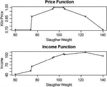
 , and g is a price function. In the present work, a price function provided by a commercial slaughterhouse was used (see Figure 1).
Commercial income function.

Three different predictive income distributions were analysed:
•
 , is the predictive income for animal i.
•
, is the predictive income for one offspring of sire i.•
is the sum of the predictive incomes for n = 500 future offspring of sire i.
 , is the predictive income for animal i.
 , is the predictive income for one offspring of sire i.
 is the sum of the predictive incomes for n = 500 future offspring of sire i.
Results and discussion
Inferences of model parameters
The estimate of the posterior mean of the environmental standard deviation based on Model 1 was 7.05 kg. In the case of Models 2 and 3, the estimated differences between sexes in posterior means of the environmental standard deviation were 0.44 and 0.38 kg (the larger value corresponds to males), respectively, with a posterior standard deviation of the difference equal to 0.04 kg and a posterior probability of differences greater than zero of 0.99 for both models. This confirms results previously reported for body weight in cattle (Garrick et al., Reference Garrick, Pollak and Quaas1989; Kizilkaya and Tempelman, Reference Kizilkaya and Tempelman2005). A plausible explanation could be a scale effect, because males reach a greater weight than females at age at slaughter (Wellock et al., Reference Wellock, Emmans and Kyriazakis2004). For batches, a wide range of posterior differences was observed for Model 2 (0.06 to 4.92 kg) and for Model 3 (0.03 to 4.19 kg). Some of these differences were even greater than those associated with sexes, and their posterior probability of being greater (or smaller) than zero was more than 0.99.
Table 1 shows MCMC estimates of posterior means and 95% highest posterior density intervals for genetic (co)variances based on Models 1, 2 and 3. The posterior mean of the additive genetic variance  was slightly larger for Model 1 than for Models 2 and 3. The estimated 95% posterior interval for
 did not include zero, supporting the existence of additive genetic control of the environmental variation. This result is in agreement with other studies that provide statistical evidence for the additive genetic control of residual variation, for adult growth in snails (Ros et al., Reference Ros, Sorensen, Waagepetersen, Dupont-Nivet, San Cristobal, Bonnet and Mallard2004), weight at 35 days in poultry (Rowe et al., Reference Rowe, White, Avendano and Hill2006), and litter size in sheep, pigs, rabbits and mice (San Cristobal-Gaudy et al., Reference San Cristobal-Gaudy, Bodin, Elsen and Chevalet2001; Sorensen and Waagepetersen, Reference Sorensen and Waagepetersen2003; Gutiérrez et al., Reference Gutiérrez, Nieto, Piqueras, Ibáñez and Salgado2006).
Monte Carlo estimates of posterior means (95% highest posterior density intervals) of genetic parameters of Models 1, 2 and 3

σ 2a = genetic variance of the mean; σ 2a* = genetic variance of the residual variance; ρ = correlation between genetic variances; h 2 = heritability for Model 1; h 211 = heritability for Models 2 and 3 (batch one, male sex); h 212 = heritability for Models 2 and 3 (batch one, female sex).
The estimate of the posterior mean of the genetic correlation (ρ) was small and the estimated 95% higher posterior density interval included the value zero. This implies a lack of (or very weak) association between the additive genes affecting the mean and those affecting environmental variance. The small negative correlation (−0.07) found between the estimated posterior means of additive values affecting mean and variance for weight in pigs is consistent with the results reported by Rowe et al. (Reference Rowe, White, Avendano and Hill2006) for body weight in broiler chickens. However, Damgaard et al. (Reference Damgaard, Rydhmer, Løvendahl and Grandinson2003) and Huby et al. (Reference Huby, Gogué, Maignel and Bidanel2003) found positive correlations for weight at birth in pigs, and Ros et al. (Reference Ros, Sorensen, Waagepetersen, Dupont-Nivet, San Cristobal, Bonnet and Mallard2004) found a high positive correlation for adult growth in snails. Nevertheless, Gutiérrez et al. (Reference Gutiérrez, Nieto, Piqueras, Ibáñez and Salgado2006) found that correlations varied widely depending on the trait considered.
Models 2 and 3 generate a covariate-related heritability, (see equation (3)). For example, Table 1 presents the posterior means of heritability of batch one for males (h 211) and for females (h 212). Figure 6 shows the frequency distribution of heritability (posterior means) for batch and sex combinations inferred from Model 3 (results were similar for Model 2). Differences between heritabilities were large, with a maximum value in females equal to 0.96, corresponding to batch 61, and a minimum value in males equal to 0.21, corresponding to batch 16. Heritabilities were very variable across batches, with slightly larger values in females than in males, in agreement with results reported by Garrick et al. (Reference Garrick, Pollak and Quaas1989) for beef cattle. As previously pointed out by Hill (Reference Hill1984), such heterogeneity in the environmental variance can seriously affect the course of the selection process. When heterogeneity is not accounted for, for a given intensity of mass selection, a higher proportion of individuals are chosen from the highly variable groups.
Histograms of heritabilities for different batches and sexes under Model 3.
Model fit and comparison
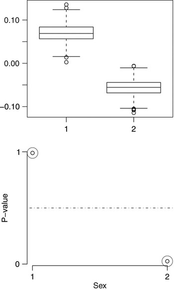
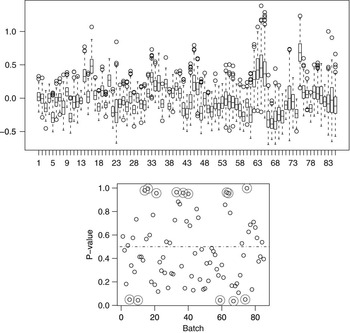
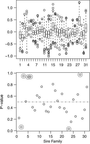
Results from the study based on posterior predictive model checking under Model 1 are shown in Figures 2–4 (see expression (7)). Figures 2–4 (upper) show the difference between the discrepancy measure evaluated using predictive (replicated) data Tjk(y rep,θ 1) and the discrepancy measure evaluated using the observed data Tjk(y,θ 1). Values larger or smaller than zero indicate a possible association between heterogeneity of environmental variance and the effect (batch, sex and sire family) studied. As a measure of the discrepancy test, Figures 2–4 (lower) show the posterior predictive P-values: the circled points indicate P-values greater than 0.95 or smaller than 0.05.
Upper: Boxplot for posterior predictive realisations of discrepancy measure under Model 1 designed to test environmental variance heterogeneity due to sex Tsk(y,θ 1) –Tsk(y rep,θ 1), k=1,2, 1: males, 2: females. Lower: Posterior predictive P-values of the discrepancy measure under Model 1 defined in expression (5).

Upper: Boxplot for posterior predictive realisations of discrepancy measure under Model 1 designed to test environmental variance heterogeneity due to batch Tbk(y,θ 1) –Tbk(y rep,θ 1), k=1,…, 85. Lower: Posterior predictive P-values of the discrepancy measure under Model 1 defined in expression (5).

Upper: Boxplot for posterior predictive realisations of discrepancy measure under Model 1 designed to test environmental variance heterogeneity due to sire family Tsfk(y,θ 1)−Tsfk(y rep,θ 1), k=1,…,32. Lower: Posterior predictive P-values of the discrepancy measure under Model 1 defined in expression (5).

Figure 2 (upper) suggests that environmental variance is greater in males than in females. The P-values provide a little more formal support, being 0.99 for males and 0.02 for females. Heterogeneity due to batch is shown in Figure 3 (upper). Due to high posterior uncertainty, there is no clear pattern of batch effect associated with the environmental variance. However, around 17% of the posterior predictive P-values are either greater than 0.95 or smaller than 0.05 (Figure 3, lower). Moreover, these results are consistent with the wide ranges of the estimates of posterior differences between batches under Models 2 and 3. Figure 4 (upper) indicates that the association between environmental variance and sire families does not have a clear pattern. Furthermore, the posterior predictive P-values (Figure 4, lower) only demonstrate heterogeneity of environmental variance for 5 out of 31 sires. In order to explore a possible association between heterogeneity of environmental variance and an additive genetic control, Figure 5 shows a plot of the posterior predictive P-value for each sire family under Model 1 v. the posterior mean of the sire additive genetic values affecting environmental variation (E(a*|y)). A linear regression is fitted and the estimate is 0.85, indicating that extreme values of the posterior predictive P-value correspond to the smallest and largest values of E(a*|y). Therefore, the heterogeneity of environmental variance associated with sire family is, to a certain degree, captured by the model that postulates that environmental variation is partly genetically controlled.
Association between posterior predictive P-values of the discrepancy measure for each sire family, under Model 1 defined in expression (5), v. posterior mean of the sire additive genetic values affecting environmental variation (E(a*|y)) under Model 3.
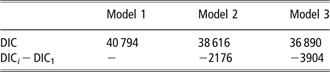
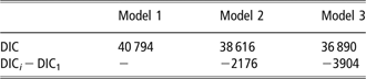
Table 2 shows the Monte Carlo estimates of the DIC for the three models, expressed as deviations from Model 1. The comparison based on DIC therefore favours Model 3 followed by Model 2. This is in agreement with the posterior predictive checks.
Natural logarithm of deviance information criterion (DIC) and differences in DIC expressed from Model 1
The study of model fit based on the posterior predictive distributions, together with the model comparison study based on the DIC, and the fact that the marginal posterior distribution of  was clearly shifted away from zero, provide support for a genetically structured environmental variance of body weight at 175 days. This opens the possibility of controlling variation for this trait by selection.
Prediction of economic income: an illustration
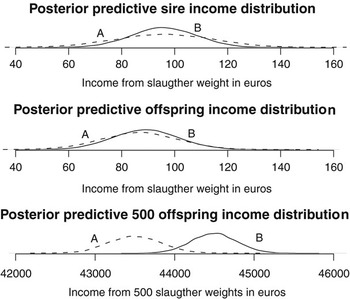
One possible implication of Model 3 in an animal breeding context is illustrated below for the case of two specific sires. Figure 7 presents three different plots of the posterior predictive income distributions for these sires. The first plot shows that the posterior predictive income distributions of the two chosen sires (A and B), have almost identical posterior means of breeding values affecting the mean (2.01 kg for sire A and 2.10 kg for sire B) but different posterior means of breeding values affecting the environmental variance (0.48 kg2 for sire A v. −0.50 kg2 for sire B). The second plot shows posterior predictive income distributions for an offspring of the two sires. Finally, the third plot shows the distribution of the sum of the economic income of 500 offspring for each sire. These plots show that while there were no important differences between predictive incomes for one offspring (second plot), there were clear differences when 500 offspring are included. The sire with smaller breeding values affecting the environmental variance (B) generates higher incomes, with a mean difference of €2 for pig (€1000 in total), which corresponds to 2.2% increased income. This shows that genetic differences at the level of environmental variation have an important effect on the economic value of a candidate for selection.
Posterior predictive incomes for two selected sires (A, B) with different breeding values for the environmental variance and their offspring.

We also compared the expected economic gain by either selecting on an index based on both breeding values (a and a*) or based only on breeding values affecting the mean (a). The computations were based on estimates of posterior means derived from Model 3. The expected response was calculated following Ros et al. (Reference Ros, Sorensen, Waagepetersen, Dupont-Nivet, San Cristobal, Bonnet and Mallard2004). We considered directional selection with a proportion selection of 10%. First, we studied selection of the highest ranking individuals based only on the posterior mean of additive genetic values controlling mean slaughter weight (i.e. E(a|y)). Changes in E(a|y) resulted in an increased in slaughter weight of 8%, without a correlated reduction in environmental variance. Second, we considered an index I=a* + k*a with k=(σ 2a*/σ 2a) that provides the same weight to both components of the index. In this case, the change in E(a|y) resulted in an increase in slaughter weight of 6% with a reduction in environmental variance of 18%. In terms of the response to selection in income (E(V|y)),selection based on the index results in approximately 0.7% more income than selection based on E(a|y). This result must be taken with caution due to the strong influence of the price function.
In conclusion, this study provides support for a model postulating that environmental variance of slaughter weight at 175 days in pigs may be partly genetically determined. This opens the possibility of controlling variation by selection. In addition, the present study indicates that prediction of future income is influenced by genes affecting both the mean and the variance. This information could be incorporated in a selection index using a given price function.
Acknowledgements
Financial support was provided by the IRTA, Spain (grant 0502-21102). The authors gratefully acknowledge the cooperative COPAGA for its collaboration and would particularly like to thank Sergi Illán, Eva Ramells, Eva Roca and Félix Grau.