1. INTRODUCTION
With the rapid development of the global economy, maritime transportation represents approximately 90% of global trade by volume. Maritime safety and security has been heavily challenged, and has brought loss of life and property, and damage to the maritime environment across the globe (Heij et al., Reference Heij, Bijwaard and Knapp2011). To improve the safety of maritime transportation and traffic, maritime surveillance systems have been installed in harbour and coastal waters. Maritime surveillance systems can be applied to achieve higher levels of situational awareness with the goal of safe and efficient maritime transportation and traffic. A major problem in maritime surveillance is that the number of vessel tracks may be very large, and they are difficult to monitor with limited maritime traffic surveillance operator resources. With the demand from maritime surveillance systems and high scales of maritime surveillance data, maritime anomaly detection has been an important research area during the last few years (Tun et al., Reference Tun, Chambers, Tan and Ly2007; Pallotta et al., Reference Pallotta, Vespe and Bryan2013; Hamed et al., Reference Hamed, Uwe and Amir2015).
Maritime anomaly detection research methods can be roughly categorised as unsupervised trajectory clustering method, statistical theory method and neural network method. Dahlbom and Niklasson (Reference Dahlbom and Niklasson2007) used spline-based clustering to solve the task of representing the normal behaviour of a vessel, then the results were applied to detect anomalous vessel behaviour. Tun et al. (Reference Tun, Chambers, Tan and Ly2007) segmented the ship trajectory into sub-trajectories and the Hide Markov Model is applied to model vessel behaviour and anomaly detection. Laxhammar (Reference Laxhammar2008) divided the surveillance waters into a small grid and used a Gaussian Mixture Model (GMM) to cluster ships’ sailing vectors in each grid, then anomaly detection in new data was performed by calculating the likelihood that was generated by the probability distributions. If the likelihood was below a certain alarm threshold, the point was considered anomalous behaviour. The typical Density-Based Spatial Clustering of Applications with Noise (DBSCAN) has been employed to cluster the vessel trajectory into the route object, waypoint object and stationary object, and construct a framework to detect the anomaly and predict ship behaviour (Pallotta et al., Reference Pallotta, Vespe and Bryan2012; Reference Pallotta, Vespe and Bryan2013). The neural network and associative rules were introduced to learn the pattern of vessels for maritime anomaly detection (Rhodes et al., Reference Rhodes, Bomberger, Seibert and Waxman2005; Reference Rhodes, Bomberger and Zandipour2007). Riveiro (Reference Riveiro, Johansson, Falkman and Ziemke2008; Reference Riveiro2014) proposed a visual analytical method to model normal behavioural models of vessel traffic and support the process of finding rare or anomalous vessel behaviour while monitoring maritime traffic. Quantitative and qualitative usability assessments were carried out and the results proved its efficiency. Jousselme and Pallotta (Reference Jousselme and Pallotta2015) dissected uncertainty-based fusion techniques for maritime anomaly detection and compared their differences and possible complementarity in uncertainty representation and expressiveness of maritime anomaly detection. Lei (Reference Lei2015) modelled vessel sailing patterns by considering the spatial, sequential and dynamic features of vessels, and defined a combined index of outlying scores to detect anomalous vessel behaviour.
The method of unsupervised clustering for anomaly detection involves automatic grouping of data into multiple clusters according to their distinguishing features, and it assumes that the clustering data reflects what is considered more or less normal. New data presented to the model is regarded as more or less anomalous based on the distance to the nearest cluster (Laxhammar Reference Laxhammar2008). During the process of maritime anomaly detection, a difficult step is the selection of feature to be clustered and the rejection of noise data. The statistical theory method needs to grid the surveillance waters and ensure every small grid element obtains enough ship trajectories to fit the statistical model, but the grid can also not be so dense as to lead to high computational complexity, thus it has to balance the two aspects, and this method is usually used within confined waters. The neural network method needs complicated training processes, and the result is sometimes uncertain. Although Pallotta et al. (Reference Pallotta, Vespe and Bryan2013) did not grid the surveillance area, this work clustered the dispersed vessel trajectory points. Actually, the vessel behaviour consists of a sequence of trajectory lines, and the point-based cluster approach partially destroys the integrity of sequential vessel behaviour, and it reduces the correlation and continuity of training vessel behaviour. Some vessel trajectories have space similarity, but may belong to a different vessel behaviour category. The point-based clustering approach may also break the dynamic characteristic of moving objects.
Based on the claims of the literature reviewed, we know the key problem of intelligent maritime surveillance is the modelling of typical sailing patterns of training vessel trajectories and classification of vessel behaviour to be monitored. The Naïve Bayes classifier is based on the theory of Bayes probability, it deduces the posterior probability from prior probability and class-conditional probability functions. The Naïve Bayes classifier is usually utilized to categorize and classify documents (Noaman et al., Reference Noaman, Elmougy, Ghoneim and Hamza2010), carry out health surveillance (Marucci-Wellman et al., Reference Marucci-Wellman, Lehtob and Corns2015) and detect internet intrusion (Mukherjee and Sharma Reference Mukherjee and Sharma2012; Varuna and Natesan Reference Varuna and Natesan2015). The Naive Bayes classifier can classify the data according its posterior probability dynamically, and its performance is accurate (Mukherjee and Sharma Reference Mukherjee and Sharma2012).
The main contribution of this paper is that we proposed a novel method combining the line-based trajectory clustering and Naïve Bayes classifier, which models the normal vessel behaviour and detects anomalous vessel behaviour in maritime surveillance. In the process of vessel trajectory clustering, the Calinski-Harabasz index is introduced to solve the difficulty of the optimal number of clusters on the basis of different combinations of spatial and directional distance. The optimal combination of k, k 1 and k 2 is obtained quantitatively. This procedure can also be applied to determine the best number of clusters on the basis of combinations of different distance, especially the clustering process of high dimensional data.
The rest of this paper is organised as follows: Section 2 describes the mathematical model and process of line-based trajectory clustering and learning of typical vessel behaviour patterns. Section 3 proposes the construction of vessel sailing behaviour of Naïve Bayes Classifier for maritime anomaly detection. Section 4 presents two experiments in the Xiamen Qingyu fairway and Chengsanjiao traffic separation scheme. The effectiveness and robustness of our proposed model are demonstrated by the results and discussions. Section 5 summarises our proposed model, describes achievements and outlines the further work.
2. LINE-BASED TRAJECTORY CLUSTERING OF TYPICAL VESSEL BEHAVIOUR
2.1. Characteristic analysis of vessel trajectory on the basis of AIS data
A vessel's sailing pattern is characterised and determined by a series of lines consisting of varying sailing trajectories in respect to space and time, which can be indicated and expressed by Automatic Identification System (AIS) data. AIS was introduced in the International Convention for the Safety of Life at Sea (SOLAS) amendment, which stated that all vessels over 300 Gross Tonnes (GT) engaged in international voyages, all cargo vessels over 500 GT and all passenger vessels are required to be equipped with AIS from 31 December 2004 (Aarsæther and Moan, Reference Aarsæther and Moan2009; Silveira et al., Reference Silveira, Teixeira and Guedes Soares2013). AIS transmits ship-related data which can be divided into three groups, including dynamic data, static data and semi-static data (Aarsæther and Moan, Reference Aarsæther and Moan2009). AIS dynamic data contains valuable information for maritime situational awareness (Mou et al., Reference Mou, Van der Tak and Ligteringen2010; Lane et al., Reference Lane, Nevell, Hayward and Beaney2010). It consists of MMSI, RECDATATIME, LONGITUDE, LATITUDE, Course Over Ground (COG) and Speed Over Ground (SOG), etc. The RECDATIME is time when the data was broadcast, LONGITUDE and LATITUDE are the position of vessel at RECDATIME, COG indicates the sailing direction of vessel over ground and SOG indicates the speed over ground. The MMSI (Maritime Mobile Service Identity) is the unique identifier of the vessel. The AIS data serve as important marine traffic input elements to assess the risk (Silveira et al., Reference Silveira, Teixeira and Guedes Soares2013; Weng and Xue Reference Weng and Xue2015; Zhang et al., Reference Zhang, Goerlandt, Kujala and Wang2016) and quantify vessel behaviour (Liu and Chen Reference Liu and Chen2013). In our study, we arrange the MMSI in the static data as an index of each vessel, and the sailing behaviour of a vessel is described below.
 $$\hbox{Trajectory}_{i} = \{(\hbox{LONGITUDE, LATITUDE, COG, SOG})_{t}\}$$
In Equation (1), the i is MMSI of vessel, t is RECDATATIME of vessel whose MMSI is i. We can see vessel trajectory has both spatial and temporal characteristics from Equation (1). In order to learn the sailing pattern of vessels from raw vessel trajectory, we take the similarity of spatial and directional characteristics of vessel trajectory into consideration. We design a method of trajectory similarity measurement which obtains both the spatial and directional characteristics of vessel trajectories.
2.2. Similarity measurement of vessel trajectory
The similarity measurement, which is also expressed in terms of distance, is the basic concept of pattern recognition. The similarity measurement is a fundamental basis to carry out the sample data clustering and classification (Bishop Reference Bishop2006; Yuan et al., Reference Yuan, Xia, Zhang and Zhou2011). There are some frequently used distance measuring methods to calculate the distance between the data of a point or line, such as Euclidean distance, Mahalanobis distance, Minkowski Distance, Longest Common Subsequence Distance and Hausdorff distance. Among these five methods, the former four methods need the line with the same number of points, but the latter Hausdorff distance does not have this requirement (Qu et al., Reference Qu, Zhou and Chen2009; Hu et al., Reference Hu, Wang, Qu and Li2011). Considering that the vessel trajectory consists of different numbers of points, we use the improved Hausdorff distance to measure the spatial similarity of vessel trajectory for the purpose of the clustering process. We also design a new method to measure the directional similarity between vessel trajectories with respect to the COG of vessel trajectory expressed by the AIS data. Then, a spatial and directional similarity measurement of vessel trajectories is proposed, so as to distinguish the difference of vessel behaviour from spatial and directional characteristics.
2.2.1. Spatial similarity of vessel trajectory based on improved Hausdorff distance
The mathematical model of Hausdorff-based distance is described as below, assuming that there are two trajectories A and B. Their spatial sequence can be expressed as
 $\hbox{A:X}_{a} = (\hbox{x}_{a1},\,\hbox{x}_{a2},\ldots, \hbox{x}_{an})^{\rm T}$
,
 $\hbox{B:X}_{b} = (\hbox{x}_{b1}, \hbox{x}_{b2}, \ldots, \hbox{x}_{bn})^{\rm T}$
, the X consists of Longitude and Latitude. The Hausdorff distance of trajectory A and B can be written as (Hu et al., Reference Hu, Wang, Qu and Li2011).
 $$d(X_a ,X_b) = \max (h(X_a ,X_b), h(X_{b}, X_a))$$
 $$h \lpar A,B \rpar =\mathop{\max}\limits_{a \in A} (\mathop{\min}\limits_{b \in B} \Vert a - b \Vert)$$
The Hausdorff distance reflects the biggest degree of mismatch between trajectories, but it only considers the maximum distance between two points which belong to two trajectories. If there are some noisy points in the trajectory, the accuracy of the distance will be compromised, and it affects the difference measurement of the trajectory. To solve this defect, we adopt the improved Hausdorff distance to express the distance between the trajectories. Assuming a i is the i th point of trajectory A, and there always exists point b j of trajectory B that satisfies the following equation,
 $$\varphi (i) = \mathop{\arg \min}\limits_{{\rm j} \in B} \Vert x_i ^a - x_j^b, y_i^a - y_j^b \Vert$$
where x i a and y i a represent the longitude and latitude of the i th point of trajectory A, x j b and y j b represent longitude and latitude of the j th point of trajectory B, which is the nearest to the i th point of trajectory A. If there are NA points in trajectory A, the improved Hausdorff distance of trajectory A to B can be defined as below.
 $$\hbox{h}(A,B) = {1 \over N_A} \sum_{{\rm i}\in A} \Vert x_i^a - x_{\varphi (i)}^b, y_i^a - y_{\varphi (i)}^b \Vert$$
As a result, the noise data has little effect on the accuracy in the improved Hausdorff distance. The improved Hausdorff distance is a directional distance, so h(A,B)≠h(B,A), so we define the maximum of h(A, B) and h(B, A) as the final spatial distance d(A, B) between trajectories A and B, and the mathematical expression is written as Equation (6).
 $$d(A,B) = \max (\hbox{h}(A,B),\,\hbox{h}(B,A))$$
2.2.2. Directional similarity of vessel trajectory
Though some trajectories have short spatial distances, they may have different moving directions, and they still have big differences. Considering the directional information expressed by COG in the AIS data, we design a directional distance expression to distinguish the different directional trajectory.
 $$d_{COG} (A,B) = \vert COG_A - COG_B \vert$$
 $$COG_A = {1 \over N_A} \sum_{i \in A} \hbox{COG}_i^A$$
 $$COG_B = {1 \over N_B} \sum_{i \in B} \hbox{COG}_i^B$$
Where the COG A and COG B are the mean COG value of trajectories A and B, and the N A and N B stand for the total number of points contained by trajectory A and B.
2.2.3. Normalisation of spatial and directional distance
In order to ensure the same numerical magnitude of two kinds of distance, we use the linear transformation to map the spatial and directional distance into the range of [0, 1] (Han and Micheline, Reference Han and Micheline2006). The mathematical formula of linear transformation is shown below,
 $$X_{norm} =(X - \min)/(\max -\min)$$
where X stands for the distance to be normalised, the max and min are the maximum and minimum value of each spatial and directional distance. After the step of linear transformation, the normalised spatial and directional distance X norm will be mapped into the range of [0,1].
2.2.4. Combined spatial and direction distance between vessel trajectories
In order to measure the distance comprehensively from the spatial and directional features of vessel trajectory, we combine the two kinds of distance and get the spatial and direction distance between vessel trajectories, and the mathematical expression is written as Equation (11).
 $$D(A,B) = k_1^{\ast} d(A,B) + k_2^{\ast} d_{COG} (A,B)$$
where the k 1 , k 2 are the weight of spatial distance and directional distance, the sum of k 1 and k 2 is 1. The value of k 1 and k 2 can be initially set according to the specific situation and characteristic of the vessel trajectories to be clustered, then the weight can be adjusted based on the satisfactory clustering experiment results. The satisfactory clustering experiments can be assessed by the theory of minimum distance within cluster and maximum distance between clusters in the clustering process. In our study, we will assign different values to the two kinds of weight, then the quality of each combination of weight in the clustering process is compared by introducing the Calinski-Harabasz index (Calinski and Harabasz, Reference Calinski and Harabasz1974). We give them preferred parameters after multiple tests, finally offering a more accurate similarity standard for clustering vessel behaviour from spatial and directional features of the vessel trajectory.
2.3. Vessel trajectory clustering based on combined spatial and directional distance
To test the results of vessel trajectory clustering based on the different weight of distance, we apply the method of hierarchical and k-medoids clustering to process the vessel trajectories. (Morris and Trivedi, Reference Morris and Trivedi2008).
2.3.1. Test the results of vessel trajectory clustering based on the different weight of distance
The hierarchical clustering does not need to know the number of clusters before it is implemented. The procedure of hierarchical clustering is detailed below.
-
Step 1. Obtain the distance matrix of vessel trajectories to be clustered. We obtain the distance matrix obtaining the combined spatial and directional distance of vessel trajectories by the means discussed in the former part.
-
Step 2. Link pairs of vessel trajectories that are close together into binary clusters according to their distance from each other.
-
Step 3. Continue to link other vessel trajectories to create bigger clusters until all the vessel trajectories in the original dataset are linked together in a hierarchical tree.
-
Step 4. Use a dendrogram to show the hierarchical tree and create the cluster.
After the process of hierarchical clustering, we can see the most preferred and probable number of clusters, and name it K pre.
2.3.2. Cluster the vessel trajectories by k-medoids
Though the hierarchical clustering can give us K pre number of clusters, we create a range of values whose centre is K pre , then we determine to use the k-medoids partition method to cluster vessel trajectories. The k-medoids procedure for clustering vessel trajectories is described as below (Han and Micheline, Reference Han and Micheline2006).
-
Step 1. Assign the number of clusters k from the result of hierarchical clustering.
-
Step 2. Calculate the combined spatial and direction distance of vessel trajectory. Assuming there are H trajectories in the training set, we will get a distance matrix L whose dimension is H by H and element L(i, j) expresses the combined spatial and direction distance between trajectory i th and trajectory j th .
-
Step 3. Assign the initial k centres randomly. Select the k centres from the H trajectories; we can set a threshold during the process and keep a distance between initial centres larger than the threshold, which can reduce the iteration times.
-
Step 4. Classify the vessel trajectory according to its distance to the initial centres, and assign the sample trajectory to the nearest cluster of initial centres. As a result, we get the initial k clusters of vessel trajectories.
-
Step 5. Readjust each cluster centre, and find the trajectory whose sum of distance to the other trajectory is the minimum, then we get the new representative centre of each cluster.
-
Step 6. Repeat Step 4 and Step 5, until the centre does not change after iterations. Finally, the trajectory is the centre of each cluster, and each cluster represents the same vessel sailing pattern.
2.3.3. Evaluation of clustering process
To assess the quality of the k-medoids clustering result, the Calinski-Harabasz index (also called Variance Criterion Ratio, VCR) is introduced to test the best number of clusters on the basis of different combination of spatial and directional distance. The Calinski-Harabasz index is defined as below,
 $${VCR}_k = {SS_B \over SS_W} \times {(N - k) \over k - 1}$$
where SSB is the overall between-cluster variance, SSW is the overall within-cluster variance, k is the number of clusters, and N is the number of observations. The overall between-cluster variance SSB is defined as
 $${SS}_B = \sum_{i = 1}^k {n_i \vert {m_i -} m \vert}^2$$
where k is the number of clusters, m i is the centroid trajectory of cluster i, m is the overall mean of the sample data, and | m i −m |2 is the norm distance between the two vectors.
The overall within-cluster variance SSW is defined as
 $${SS}_W = \sum_{i = 1}^k \sum_{x \in c_i} \vert x - m_i \vert^2$$
The well-defined clusters will have a large between-cluster variance (SSB) and a small within-cluster variance (SSW). The larger the VCR, the better quality of the clustering result and parameter set. To determine the optimal number of clusters and preferred weight of two kinds of distance, we maximise VCR with respect to k (number of clusters), k 1 and k 2 . At last, the optimal number of clusters and the preferred combination of k 1 and k 2 are obtained by the solution with the highest Calinski-Harabasz index value.
The overall procedure of obtaining the preferred k, k 1 and k 2 is summarised as below.
-
Step 1. Obtain the K pre from the graph of dendrogram in the process of hierarchical clustering.
-
Step 2. Create the range of values which vary from K min to K max , whose centre is K pre . The K min and K max are set according to the possible range of number of clusters seen from the dendrogram in the process of hierarchical clustering.
-
Step 3. Design the cases of different combination of k 1 and k 2 , and we assume that there are n cases consisting of different k 1 and k 2 .
-
Step 4. For each k=K min :K max
-
For case i=1:n
-
The k-medoids is applied to cluster vessel trajectories on the basis of parameter (k, i).
-
Calculate the Calinski-Harabasz index of result(k, i).
-
-
End
-
-
End
-
Step 5. The optimal clustering result is obtained through the maximum Calinski-Harabasz(k, i), thus, the optimal vessel trajectories clustering result will be obtained.
3. CONSTRUCTION OF NAÏVE BAYES CLASSIFIER FOR ANOMALOUS VESSEL BEHAVIOUR DETECTION
3.1. Theory of Naïve Bayes classifier for sailing behaviour of vessel
Classifying and judging the vessel behaviour to be monitored in respect of the typical historical vessel voyage behaviour within the sea area is a key technique in intelligent marine surveillance study. If the vessel behaviour belongs to the existing historical vessel sailing pattern, the vessel behaviour will be a normal behaviour. If the vessel sailing behaviour deviates from their original behaviour pattern or does not belong to any existing navigation behaviour model, then the behaviour will be identified as an anomalous sailing behaviour. According to the description of the marine anomaly detection process, we use a Naïve Bayes classifier to categorize the vessel behaviour.
Assuming that we get n types of typical vessel sailing patterns after trajectory clustering, we name them as
 $C_{{1}},C_{{2}},{\ldots}C_{n}$
. In order to match the vessel behaviour to be monitored with the existing typical vessel pattern, we use a Naïve Bayes classifier to design the vessel behaviour classifier. For each arbitrary vessel trajectory X to be monitored, the probability that it belongs to the typical vessel pattern Cj can be calculated using Equation (15),
 $$P(C_{\rm j} \vert x_m ) = {P(C_j) P(x_m \vert C_j) \over \sum_{i = 1}^n P(C_i) P(x_m \vert C_i)}$$
where x
m
is the number m point of trajectory X, P(C
j
) is the prior probability of typical vessel pattern C
j
obtained by trajectory clustering, and the
 $P(x_{m} \vert C_{j})$
is the probability density function of x
m
belonging factor to the C
j
. The principle of the Naïve Bayes classifier is to calculate the posterior probability through the prior probability and class-conditional density function, and the object to be classified will belong to the class which has the largest posterior probability. For a specific classification test sample, the value of the denominator is fixed, so the maximum posterior probability for the test sample data is equivalent to the maximum numerator value of the Bayesian formula, namely maximum product value of prior probability and conditional probability. It can be expressed as below,
 $$C_{MAP} = \mathop{\arg \max}\limits_{c_j, \,j\in [1,n]} P(C_j \vert x_m) \propto \mathop{\arg \max}\limits_{c_j,\,j \in [1, n]} P(x_m \vert C_j) P(C_j)$$
During the process of data classification, test samples will be classified into the class of C
MAP
. In Equation (15), the prior probability P(C
j
) can be obtained by the results of vessel trajectory clustering, and the class-conditional probability function
 $P(x_{m} \vert C_{j})$
is usually categorised by a multi-dimensional Gaussian probability function.
3.2. Estimation of parameter for class-conditional density function in Naïve Bayes classifier
When constructing the vessel behaviour Naïve Bayes classifier, we should obtain the prior probability and class-conditional density function of each cluster of vessel behaviour. The prior probability of each cluster can be obtained by the statistics of trajectory clustering, and the class-conditional density function
 $P(x_{m} \vert C_{j})$
is usually fitted by a multi-dimensional Gaussian distribution in the Bayes classifier. The format of
 $P(x_{m} \vert C_{j})$
can be written as Equation (17).
 $$P(x_m \vert C_{\rm j}) = {1 \over 2\pi^{n/2} \vert S_j \vert^{1/2}} \exp \left[-{1 \over 2} (x_m - \mu_j)^T S_j^{-1} (x_m - \mu_j) \right]$$
where μ
j
is the mean vector of each vessel trajectory cluster C
j
,
 $S_{j} = E[(X - \mu_{j}) (X - \mu_{j})^T]$
is the two- dimensional covariance matrix, n is number of vessel trajectories.
As can be seen, the multidimensional Gaussian distribution is characterised by a mean vector and covariance matrix, and they can be estimated by the maximum likelihood estimation method (Bishop, Reference Bishop2006; Laxhammar, Reference Laxhammar2008):
 $$\left\{\matrix{\hat{\mu} = {1 \over n} \displaystyle\sum_i^n {X_i} = \bar{X} \hfill \cr \hat{S}_j = {1 \over n} \displaystyle\sum_{i=1}^n {(X_i -\bar{X})} (X_i - \bar{X})^T} \right.$$
We use the line-based vessel trajectory clustering method to model the normal data, then the Naïve Bayes classifier is applied to classify and detect the anomalous vessel trajectory. For any vessel trajectory to be monitored, the Naïve Bayes classifier will put it into a certain trajectory cluster according its posterior probability in respect of each historical typical trajectory cluster. When the vessel trajectory does not belong to any normal and typical vessel trajectories cluster or deviates from one cluster to another cluster, then it will be identified as anomalous behaviour and the operator on watch can be automatically alerted in the maritime traffic surveillance system.
4. EXPERIMENTAL CASE STUDIES
In order to verify the effectiveness of the proposed methodology, we carried out two experiments in different waters of China. The first one is the Qingyu fairway in Xiamen Bay China, shown in Figure 1, and the second one is the waters of Chengsanjaio, China, shown in Figure 14. In these two experiments, the AIS data is supplied by the Integrated Vessel Information Service System (IVISS) (Shao et al., Reference Shao, Sun, Pan and Ji2007).
Qingyu fairway of Xiamen Bay.

4.1. A case study within waters of Xiamen bay
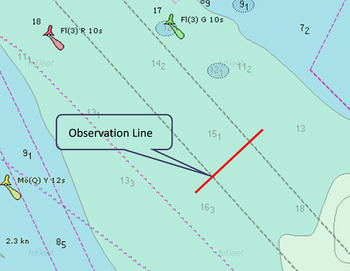
Figure 1 depicts information on Qingyu fairway within Xiamen Bay, China. The preferred navigational waters are constrained by the dark dashed line and the channel is in the middle of the red and green navigational buoy in Figure 1.
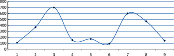
The Qingyu fairway is the main channel into Xiamen port. There is no traffic separation scheme established in the Qingyu fairway, and theoretically, vessels can sail along any space within these waters. However, according to Rule 9 of the Regulations for Preventing Collisions at Sea, 1974 (COLREGS), a vessel proceeding along the course of a narrow channel or fairway shall keep as near to the outer limit of the channel or fairway which lies on her starboard side as is safe and practicable. But what is the lateral distribution of vessel sailing position within the fairway? In order to answer this question, we set a line of observation which is perpendicular to the direction of main traffic flow, and then characterise the transverse position distribution of vessel traffic flow by calculating the number of vessels within each interval of line according to the dynamic and static AIS data lasting five days by the method developed by (Zhen et al., Reference Zhen, Shao, Pan and Zhao2015). The result is shown in Figure 2.
Vessel trajectories lateral distribution in Qingyu fairway.

As can be seen from Figure 2, the intervals No.3 and No.7 are the peak values of transverse position distribution of vessel traffic flow and the length of these vessels is between 100 m and 200 m. The interval 5 is also a smaller peak interval and the length of these vessels is more than 250 m (See more details in Zhen et al., Reference Zhen, Shao, Pan and Zhao2015). These vessels navigate close to the middle of Qingyu fairway because their draught is so deep and they have to keep enough under keel clearance in the central area of the fairway. Thus we know that the lateral distribution of vessel trajectory varies according the static characteristics of vessel. So the spatial distribution of vessel trajectories is complex with respect to the static characteristics of the vessel.
Based on the information from the study of vessel lateral position distribution and its relation to the length of vessel, we select the most proportional vessel trajectories sailing in the scope of Qingyu fairway whose length is between 100 m and 200 m and some vessels which sail across the Qingyu fairway from the south east as the training data to be clustered. The original ship trajectories in Qingyu channel are plotted in Figure 3 after pre-processing.
Original ship trajectory distribution within Qingyu fairway.

4.1.1. Vessel trajectory clustering and assessment with the different weight of spatial and directional distance
After calculating and normalizing the spatial and directional distance between training vessel trajectories, we try to assign the different weights of spatial and directional distance during the clustering process. As mentioned before, the sum of k 1 and k 2 is 1, the value of k 1 (weight of spatial distance) varies from 0 to 1 and the value of k 2 (weight of directional distance) varies from 1 to 0. We divide it into five cases, and design the combined value of k 1 and k 2 shown in Table 1.
Weight of spatial and directional distance.

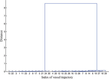
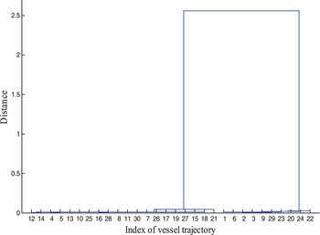
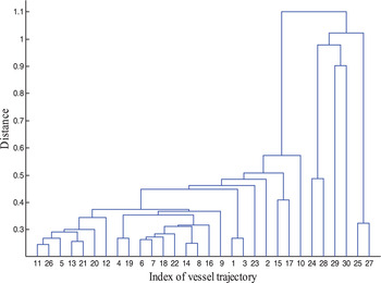
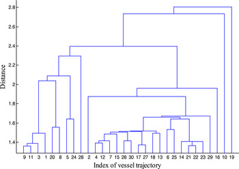
According to the cases of weight in Table 1, we use the hierarchical clustering to cluster the vessel trajectory. The results are shown in Figures 4–8.
Case 1 (0,1).

Case 2 (0.3,0.7).

Case 3 (0.5, 0.5).

Case 4 (0.7, 0.3).

Case 5 (1,0).

From the results shown in Figures 4 and 5, we know that when the value of k
2
(weight of directional distance) is between 0.7 and 1, the vessel trajectory can be clustered into two clusters. Once the weight of k
2
is set between 0 and 0.3, the vessel trajectories are difficult to cluster which can be seen in Figures 7 and 8, where there is little difference between each cluster. Only when the
 $k_{1} = k_{2} = 0.5$
, the trajectories can be clustered into 3 clusters shown by Figure 6.
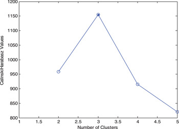
According to the dendrogram in the process of hierarchical clustering, we set a range of [2, 5] as the possible optimal choice of number of cluster, whose centre is three. Then we use the k-medoids method to cluster the vessel trajectories with the different combination of k, k 1 and k 2 . Finally, the Calinski-Harabasz index is highest when the k 1 =k 2 =0.5, and the best number of clusters is three, which is tested between two and five in the experiments shown in Figure 9.
Calinski-Harabasz index.

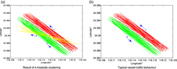
After assigning three to the number of clusters, the vessel trajectories have been partitioned into three clusters clearly shown by Figure 10(a). The three clusters corresponding to arriving vessels are plotted by red lines, while leaving vessels are plotted in green and crossing vessels are plotted in yellow. The arriving and leaving vessels are the main component of traffic flow in these waters (Zhen et al., Reference Zhen, Shao, Pan and Zhao2015), so after eliminating the crossing vessel trajectories, we treat arriving and leaving vessel trajectories as the typical vessel traffic behaviour shown in Figure 10(b). They are the training set of Naïve Bayes Classifier to classify and detect anomalous vessel behaviour.
Trajectory clustering result in Qingyu fairway.

4.1.2. Construction of Naïve Bayes Classifier within Xiamen Bay
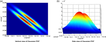
Firstly, we use the maximum likelihood estimation method to estimate the training samples and obtain the parameter of multi-dimensional Gaussian probability density distribution function of leaving and arriving vessel trajectories. The three-dimensional probability density distribution function is plotted in Figure 11.
Gaussian PDF of vessel trajectories.

In Figure 11, the dense area identifies the extent of probability distribution of vessel trajectories, the more deep the colour, the larger the probability of vessel trajectory. The two dense areas represent the leaving and arriving vessel trajectories and they correspond to the spatial distribution of the original trajectories. This means the multidimensional Gaussian probability density distribution function can quantify the spatial probability of vessel trajectories within Qingyu fairway in Xiamen bay.
4.1.3. Classification and detection of anomalous vessel behaviour within Xiamen Bay
We construct the Naïve Bayes Classifier to detect anomalous vessel trajectories when leaving and arriving from Xiamen port. During the anomaly detection process, we need to calculate the posterior probability of each point of vessel trajectory corresponding to the training set of leaving and arriving vessel trajectories. Assuming the posterior probability of the i th point with respect to the two training sets are P(Out| X i ) and P(In|X i ) respectively, we compare the values of P(Out| X i ) and P(In| X i ) and assign the point i into the cluster whose posterior probability is bigger. We set the following principle,
If (P(In| X i )>P(Out| X i ))
The trajectory point X i will be identified as triangle and indicate that X i belongs to arriving vessel behaviour;
Else
The trajectory point X i will be identified as circle and indicate that X i belongs to leaving vessel behaviour.
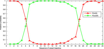
In Figure 12, there is a vessel sailing into Xiamen port, its posterior probability corresponds to the leaving and arriving training vessel trajectory changes depicted in Figure 13.
Vessel anomalous behaviour detection within Xiamen Bay.

Posterior probability changing process of monitoring ship.

As can be seen in Figure 12, the vessel trajectory to be monitored is initially sailing within the area of arriving vessel trajectory cluster and
 $P({In} \vert X_{1,2,3,4,5}) \gt P(Out \vert X_{1,2,3,4,5})$
in Figure 13, so the points from No.1 to No.5 sail according to normal behaviour of arriving vessels. Then the vessel trajectories yaw to the port side of fairway, the
 $P({In} \vert X_{6}) \lt P({Out} \vert X_{6})$
, its trajectory has been plotted as a circle in Figure 12, meaning that the vessel trajectory belongs to the leaving vessel trajectory from the No.6 point. This process indicates that the belonging factor of vessel behaviour according to the two training sets has changed. Actually, during this surveillance process the vessel yaws and invades the waters for a leaving vessel.
After the change of belonging factor of Naïve Bayes classifier of vessel trajectory, we would define the vessel behaviour as anomalous and trigger an automatic alarm to the surveillance operator. During the period, if there is a leaving vessel coming in the near future, this yawing would cause a situation of close-quarter situation or risk of collision, which will reduce the level of safety and efficiency within the port waters. When anomalous vessel behaviour occurs, the operator would advise the ship officer to alter course and sail back into its original waters, then the vessel would sail along the arriving vessel lane again.
4.2. A case study within the waters of Chengsanjiao
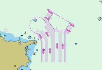
In order to test the applicability of our method in a more complicated maritime traffic situation, we carried out another experiment within the waters of Chengsanjiao traffic separation scheme. The traffic separation scheme is shown in Figure 14, and our experiment is carried out within this sea area.
Waters of Chengsanjiao.

The waters of Chengsanjiao is the sea-route which must be sailed by vessels sailing in and out of Bohai and the northern part of the Yellow Sea port, and it is a maritime traffic throat of China. On 1 December 2000, the Chengshanjiao ship routing system and ship reporting system was implemented formally after approval by the International Maritime Organization (IMO) to ensure the safety and efficiency of maritime traffic within the waters of Chengsanjiao. With the rapid growth of maritime traffic during the last decades, the former ship routing system and ship reporting system faced great challenges. The new traffic separation scheme and ship reporting system was established on 1 June 2015.
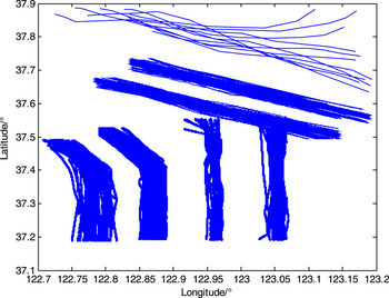
We selected the vessel trajectories which sail within and outside of the traffic separation scheme as the training data to be clustered and modelled. The length of these vessels is above 150 m to ensure that the large cargo vessels usually comply with the navigation rule of ship routing system while navigating in the waters of the routing system. The original vessel trajectories within Chengsanjiao are plotted in Figure 15.
Original vessel trajectories within Chengsanjiao.

4.2.1. Vessel trajectory clustering and construction of Naïve Bayes classifier
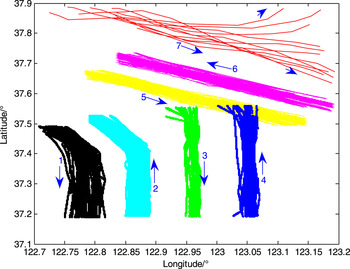
The spatial and directional distances between training vessel trajectories are calculated and normalised using the method discussed in Section 2. Then the vessel trajectories are clustered using the hierarchical clustering with the different combined weight of two kinds of distance, and at the same time, the results are assessed by the Calinski-Harabasz index in every case. When k 1 =0.7, k 2 =0.3 and the number of clusters is seven, the Calinski-Harabasz index is the largest in the experiments. So the vessel trajectories are clustered into seven clusters within the Chengsanjiao. The final results are shown in Figure 16.
Result of k-medoids clustering for Chengsanjiao.

As can be seen in Figure 16, the original vessel trajectories are partitioned into seven clusters by using the k-medoids method, and the directional characteristic of each cluster is shown by an arrow. The clusters from No.1 to No.6 are the vessel trajectories that sail complying with the Chengsanjiao traffic separation scheme, and cluster No.7 is the vessel trajectories that do not sail complying with the Chengsanjiao traffic separation scheme; these vessels sail in the directions of NE and SE.
In order to test the effectiveness of our method on the typical vessel behaviour within the Chengsanjiao traffic separation scheme, the clusters from No.1 to No.6 of vessel behaviour are treated as the training set of Naïve Bayes Classifier to identify and detect the anomaly vessel behaviour in this area of waters, and the training data is shown in Figure 17.
Typical vessel traffic behaviour within Chengsanjiao.

4.2.2. Classification and detection of anomalous vessel behaviour within Chengsanjiao
After the process of clustering, we obtained the typical vessel trajectories which are utilised to construct the Bayes Classifier within the Chengsanjiao traffic separation scheme. The six clusters of typical vessel behaviour appear even, and prior probability of each typical vessel is one in six. The class-conditional density function is fitted by a multi-dimensional Gaussian probability density distribution function, and their parameters are estimated by the maximum likelihood according to spatial distribution of typical vessel trajectories. Finally, the Bayes Classifier is applied to classify and detect anomalous vessel behaviour.
The rule of anomalous vessel detection is similar to the case study of Xiamen Bay. When the vessel sails into the Chengsanjiao waters, the Naïve Bayes Classifier will detect and classify its sailing behaviour into the existing typical behaviour within waters according to its posterior data with respect to six typical vessel sailing behaviour. We assume that the posterior probability of the i th point of vessel trajectory to be monitored in respect to the six typical sailing behaviour are namely P(1|X i ), P(2|X i ), P(3|X i ), P(4|X i ), P(5|X i ) and P(6|X i ). The point i th will be classified into the clusters whose posterior probability is maximum. During the process of vessel traffic surveillance, once the belonging factor of vessel trajectories changed, that vessel behavior would be identified as anomalous behaviour.
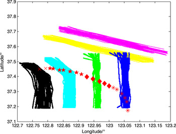
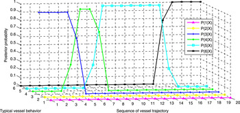
In Figure 18, a vessel sails into the traffic separation scheme of Chengsanjiao, the Naïve Bayes classifier is applied to classify its “belonging factor” to the typical sailing pattern within the waters of Chengsanjiao, its posterior probability corresponding to the six training vessel trajectories have been shown in Figure 19.
Vessel anomaly behaviour detection within Chengsanjiao.

Posterior probability changing process of monitoring vessel within Chengsanjiao.

In Figure 18, initially the vessel trajectory to be monitored is sailing to the north direction within No.3 typical sailing behaviour, and the P(3|X 1,2,3,4) is the maximum probability, the vessel is correctly classified into the No.3 typical sailing behaviour by Naïve Bayes Classifier seen in the Figure 19. As time progresses, the vessel yaws to the port side waters, and the value of P(3 | X 5, 6) decreases, then the P(4|X 6) is the maximum probability, at this time, the vessel being monitored is classified into the No.4 typical sailing behaviour from its sixth point, so the belonging factor of vessel trajectory according to the six training vessel behavior has changed. Actually the vessel sails into the southward lane, so the vessel is identified as having anomalous behaviour. Afterwards the vessel invades the No.5 and No.6 typical sailing behaviour area, and the change has been correctly detected by the Naïve Bayes Classifier according its posterior probability in respect to the training set within the Chengsanjiao separation scheme sea area.
Through this experiment in the waters of Chengsanjiao, we show the applicability and robustness of our vessel trajectory clustering and Bayes Classifier method in the maritime anomaly detection area within a more complicated maritime situation.
5. CONCLUSION
This paper proposed a new approach to detect maritime anomalies based on a combination of vessel trajectory clustering and Naïve Bayes Classifier. The case studies demonstrate the effectiveness of the presented approach to solve the maritime trajectory anomaly detection problem within Ximen Qingyu fairway and traffic separation scheme of Chengsanjiao, when a vessel deviates from its original behaviour over time. The results verified the robustness and applicability of our proposed method in the different conditions. The proposed methodology can be embedded in intelligent maritime surveillance systems, in order to improve maritime situational awareness and reduce operator workload.
In the process of vessel trajectory clustering, the Calinski-Harabasz index was introduced to solve the difficulty of the optimal number of clusters on the basis of different combinations of spatial and directional distance, while the optimal combination of k, k 1 and k 2 was obtained quantitatively. This theory can also be applied to determine the best number of clusters on the basis of a combination of different distances, especially for the clustering process of high dimensional data.
We will test the applicability of our proposed method in more complicated maritime environments, and the parameters of the cluster process will be adjusted and optimised in follow-up studies. We are also going to use our methodology to predict vessel behaviour in future research.
ACKNOWLEDGEMENTS
We would like to give thanks to the anonymous reviewers for their suggestions and promotion to our research. The research described in this paper is supported by China Scholarship Council (Grant number 201608310093), Science and Technology Committee of Shanghai Municipal (Grant number 15590501600) and Natural Science Foundation of Fujian Province of China (Grant number 2015J01214).