





1. Introduction
The Antarctic firn layer, representing the transitional zone between fresh snow and glacial ice, plays a critical role in surface mass balance, ice-sheet dynamics and the interpretation of ice-core records (Arthern and others, Reference Arthern, Vaughan, Rankin, Mulvaney and Thomas2010; Ligtenberg and others, Reference Ligtenberg, Kuipers Munneke and ven den Broeke2014). Accurate characterization of the firn’s elastic and structural properties is therefore essential for constraining firn densification processes, refining surface mass-balance models and improving the precision of satellite altimetry corrections (Medley and others, Reference Medley, Lenaerts, Dattler, Keenan and Wever2022).
Seismic exploration is an effective geophysical approach for firn structure imaging (Li and others, Reference Li, Liu, Zou, Cui, Zheng and Wang2025). Active seismic excitation generates seismic waves that propagate through the firn layer, producing surface waves, P-guided waves and first arrivals. Inversion of these signals enables the characterization of shallow subsurface structures in terms of shear-wave and compressional-wave velocities (Yang and others, Reference Yang2024). Furthermore, empirical relationships allow the estimation of firn density and porosity, providing multidimensional elastic information and valuable insights into the deeper ice structure (Anandakrishnan and Alley, Reference Anandakrishnan and Alley1997; Hempel and others, Reference Hempel, Thyssen, Gundestrup, Clausen and Miller2000; Horgan and others, Reference Horgan, Anandakrishnan, Alley, Burkett and Peters2011; Picotti and others, Reference Picotti, Vuan, Carcione, Horgan and Anandakrishnan2015; Zhang and others, Reference Zhang, Nakata, Karplus, Kaip and Yi2022; Picotti and others, Reference Picotti, Carcione and Pavan2024; Zhang and others, Reference Zhang2024).
However, conducting active-source seismic surveys in Antarctica remains challenging because artificial-source deployment and repeated source excitation are strongly constrained by extreme environmental conditions and logistical limitations. This source-side difficulty motivates passive seismic approaches, which use naturally or anthropogenically generated ambient vibrations instead of artificial source excitation. By continuously recording ambient vibrations with nodal geophones and applying coherence-based interferometric processing, virtual shot gathers can be reconstructed to enable the inversion of shear-wave structures (Claerbout, Reference Claerbout1968; Rickett and Claerbout, Reference Rickett and Claerbout1999; Schuster, Reference Schuster2001; Wapenaar, Reference Wapenaar2004; Wapenaar and Fokkema, Reference Wapenaar and Fokkema2006; Wapenaar and others, Reference Wapenaar and Fokkema2006, Reference Wapenaar, Slob and Snieder2008, Reference Wapenaar, Draganov, Snieder, Campman and Verdel2010). These developments highlight the potential of passive-source methods for complementing active-source seismic experiments, showing that surface-wave inversion from ambient noise can successfully constrain firn anisotropy, porosity and seasonal variability in Antarctica and Greenland (Diez and others, Reference Diez2016; Chaput and others, Reference Chaput2018; Lombardi and others, Reference Lombardi, Gorodetskaya, Barruol and Camelbeeck2019; Smith and others, Reference Smith2021; Chaput and others, Reference Chaput, Aster, Karplus and Nakata2022; Fu and others, Reference Fu2022; Zhou and others, Reference Zhou, Butcher, Brisbourne, Kufner, Kendall and Stork2022; Nakata and others, Reference Nakata2023; Chen and others, Reference Chen, Yan, Yang, Huang and Li2024; Pearce and others, Reference Pearce2024). Passive seismic methods based on ambient noise have been widely used due to their low cost, operational flexibility and minimal environmental disturbance. However, the frequency content of ocean microseisms is typically below 1 Hz, providing insufficient resolution for the upper tens of meters. In addition, noise sources in Antarctica often lack spatial and temporal stability, limiting the repeatability and accuracy of the retrieved wavefields.
(a) Location of the study area in Antarctica (red rectangle) and the regional elevation map, with the yellow triangle indicating the position of the survey line. (b) Spatial relationship among the drilling site, the linear array of geophones and the highway. (c) Distribution of the survey line and the borehole. (d) SmartSolo IGU-16HR single-component geophones deployed along the survey line. (e, f) Two types of heavy tracked vehicles commonly used in Chinese Antarctic expeditions: PB300 and CAT.

Figure 1 Long description
The figure presents six panels labeled a through f, documenting the field setup for vibration monitoring during subglacial drilling in Antarctica. Panel a shows a regional elevation map of the Antarctic study area. The map includes a color scale representing elevation values and labels Zhongshan Station as a key reference location. A triangle marker indicates the position of the survey line within the mapped region. Panel b is a schematic diagram showing the spatial relationship among the drilling site, the geophone array and the highway. The schematic shows a linear arrangement of geophone markers positioned symmetrically along the survey line. The drilling point is labeled with its coordinates 69°35′7″S and 76°23′7″E, with an elevation of 692.7 meters. The highway is represented as a diagonal line crossing the survey array. Geophone markers are shown at variable intervals, including 20 m and 80 m along both sides of the drilling point, with a label indicating the Chinese-Russian inland highway. Panel c is a map showing the distribution of the survey line and the borehole location relative to Zhongshan Station and the surrounding terrain. The drilling point is marked and labeled. Panel d shows a SmartSolo IGU-16 HR single-component geophone unit placed on a snow surface, with a cable visible. Panel e shows a large tracked vehicle, identified as a PB300, photographed outdoors in a snowy setting. Panel f shows another tracked vehicle, identified as a CAT, also photographed in a snowy outdoor setting.
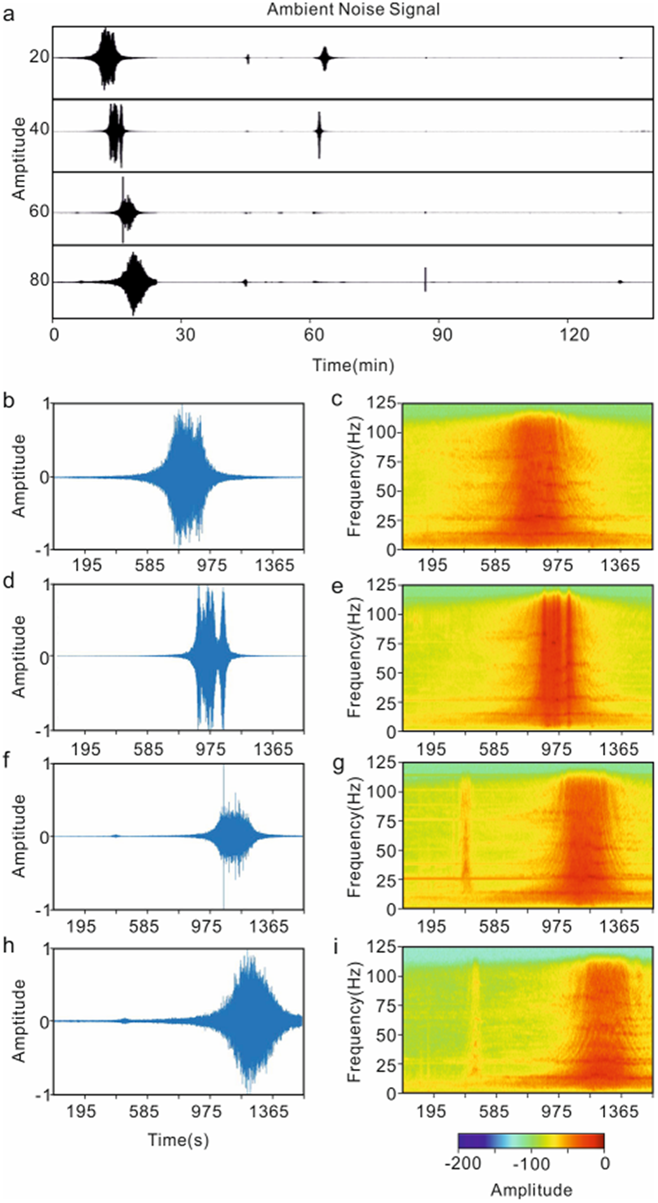
(a) Raw ambient noise records from channels 20, 40, 60 and 80. (b), (d), (f) and (h) Seismic signals associated with traffic events recorded at channels 20, 40, 60 and 80, respectively. (c), (e), (g) and (i) Corresponding time–frequency spectra obtained using windowed Fourier transforms.

Figure 2 Long description
The image contains nine panels labeled a–i. Panel a shows raw ambient noise records from channels 20, 40, 60 and 80. The horizontal axis is Time (min), ranging from 0 to 135 min, and the vertical axis is Amplitude, with the four traces vertically separated and labeled by channel number. Short-duration traffic-related bursts appear at different times in the records. Panels b, d, f and h show seismic signals associated with traffic events recorded at channels 20, 40, 60 and 80, respectively. Their horizontal axes show Time (s), ranging approximately from 195 to 1365 s, and their vertical axes show Amplitude. The traffic-event waveform appears as a localized burst in each panel, with the main burst occurring progressively later from channel 20 to channel 80. Panels c, e, g and i show the corresponding time–frequency spectra obtained using windowed Fourier transforms for the signals in panels b, d, f and h. Their horizontal axes show Time (s), and their vertical axes show Frequency (Hz), ranging from 0 to 125 Hz. Each spectrum shows a time-localized broadband energy band associated with the traffic event. A horizontal color scale labeled Amplitude is shown below the spectra, with values ranging from approximately −200 to 0. Overall, the figure shows that the recorded traffic-induced noise contains broadband energy and that the event arrival time varies systematically among the four channels.
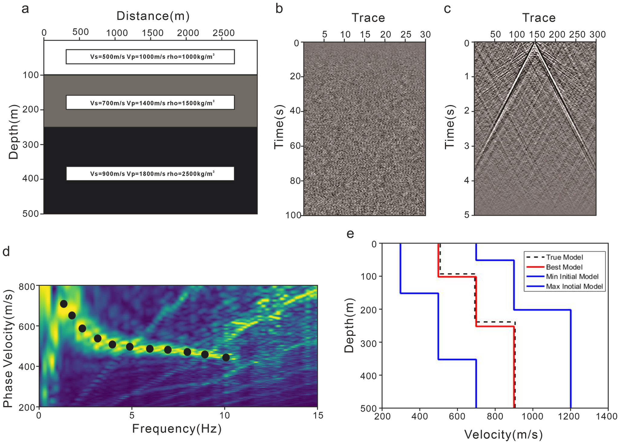
(a) Three-layer velocity model. (b) Synthetic random-noise records for a 100 s recording window. (c) Virtual-shot gather reconstructed by cross-coherence interferometry using trace 150 as the virtual source. (d) Dispersion-energy image of the virtual-shot gather and the picked fundamental-mode surface-wave dispersion curve. (e) Comparison of the inverted Vs structure with the true model and the initial model.

Figure 3 Long description
The image contains five panels labeled a–e, illustrating a synthetic validation workflow for passive-source surface-wave inversion. Panel a shows a three-layer velocity model. The horizontal axis is Distance (m), and the vertical axis is Depth (m), ranging from 0 to 500 m. Three horizontal layers are shown, with text boxes indicating the layer properties: Vs = 500 m/s, Vp = 1000 m/s and ρ = 1000 kg/m³ in the shallow layer; Vs = 700 m/s, Vp = 1400 m/s and ρ = 1500 kg/m³ in the middle layer; and Vs = 900 m/s, Vp = 1800 m/s and ρ = 2500 kg/m³ in the deepest layer. Panel b shows synthetic random-noise records for a 100 s recording window. The horizontal axis is Trace, with tick marks from about 5 to 30, and the vertical axis is Time (s), ranging from 0 to 100 s. The record appears as dense random fluctuations over the full time window. Panel c shows a virtual-shot gather reconstructed by cross-coherence interferometry using trace 150 as the virtual source. The horizontal axis is Trace, with tick marks from about 50 to 300, and the vertical axis is Time (s), ranging from 0 to 5 s. Coherent wave arrivals form a V-shaped pattern centered near trace 150, with arrivals extending to later times toward both smaller and larger trace numbers. Panel d shows the dispersion-energy image of the virtual-shot gather and the picked fundamental-mode surface-wave dispersion curve. The horizontal axis is Frequency (Hz), ranging from 0 to 15 Hz, and the vertical axis is Phase Velocity (m/s), ranging from 200 to 800 m/s. Black circular markers indicate the picked dispersion curve, which decreases from about 700–750 m/s at low frequency to about 450 m/s at higher frequency. Panel e compares the inverted Vs structure with the true model and the initial model range. The horizontal axis is Velocity (m/s), and the vertical axis is Depth (m), ranging from 0 to 500 m. The dashed black line represents the true model, the red solid line represents the best inverted model, and the blue step-like curves represent the minimum and maximum initial models. The best model generally follows the three-layer true model.
Recent studies have highlighted seismic noise generated by road vehicles and trains as an effective alternative passive source for near-surface investigations. Traffic noise typically excites higher-frequency surface waves, providing improved resolution in the shallow subsurface. Moreover, traffic flows are spatially constrained along roads and railways, offering partially controlled source azimuth and temporal repeatability (Nakata and others, Reference Nakata, Snieder, Tsuji, Larner and Matsuoka2011; Quiros and others, Reference Quiros, Brown and Kim2016; Zhang and others, Reference Zhang, Li, Wang and Wang2020; Yuan and others, Reference Yuan, Lellouch, Clapp and Biondi2020; Rincon, Reference Rincon2021; Liu and others, Reference Liu, Yue, Li and Luo2021a, Reference Liu, Yue, Luo and Li2021b, Reference Liu, Yue, Luo and Li2021c; Cao and others, Reference Cao, Huang, Hu, Xu, Tang and Yao2022; Mi and others, Reference Mi2022; Ning and others, Reference Ning, Xia, Dai, Liu, Zhang and Xi2022; Liu and others, Reference Liu, Wang, Chen and Bian2023; Liu and others, Reference Liu, Li, Yuan, Noh and Biondi2025; Xiong and others, Reference Xiong, Deng, Wang, Ye and Zhang2025).
In Antarctica, heavy snow vehicles such as the PB300, with a mass exceeding 35 t, can generate strong traffic-induced vibrations when traveling in convoys. Compared with natural sources of seismic noise such as icequakes, sea-ice melting, ocean waves and station activities, these anthropogenic signals are characterized by higher frequencies, stronger energy and more constrained source directionality. Such features provide a new perspective for shallow imaging of the Antarctic ice sheet. During the 40th Chinese National Antarctic Research Expedition in 2023, a linear seismic array consisting of 100 geophone nodes was deployed in the Larsemann Hills region of East Antarctica. The survey line, ∼2 km in length, intersects the highway used by the joint Chinese–Russian inland expedition convoys at a slight oblique angle. The array successfully recorded vibration noise signals generated by the passage of the large vehicle convoy. Based on these data, this study aims to extract surface-wave information and perform shear-wave velocity inversion. Taking into account convoy velocity, survey-line orientation and related parameters, the stationary-phase zone calculation method developed for high-speed railway noise imaging (You and others, Reference You, Mi, Guan, Zhang and Liu2023) was applied to select signal segments for coherent stacking. This approach enables the reconstruction of virtual shot gathers with clear surface-wave energy and identifiable P-guided-wave arrivals. In the present study, only the surface-wave dispersion is used for shear-wave velocity inversion, whereas the P-guided-wave arrivals are identified as coherent high-velocity phases and retained as a potential constraint for future joint inversion. The inverted shear-wave velocity structure agrees well with the borehole-constrained firn–ice stratigraphy obtained from the joint Chinese–Russian drilling project.
Initial model parameters and inversion settings.

Table 1 Long description
The table lists per-layer constraint ranges used for an inversion: lower and upper limits for shear-wave velocity, compressional-wave velocity, and layer thickness, plus density and iteration count where provided. Shear-wave velocity bounds generally increase with layer number, starting near 1400 to 1443 m/s in layers 1 and 2 and reaching about 2100 to 2309 m/s by layer 20. Compressional-wave velocity limits are 1000 to 2500 m/s for layers 1 and 2, shift to 1000 to 3000 m/s for layers 3 to 5, then to 1000 to 4000 m/s for layers 6 to 9. From layer 10 through 18, compressional-wave velocity is constrained to 3500 to 4000 m/s, and layers 19 and 20 narrow to 3800 to 4000 m/s. Layer thickness limits are constant across all layers at 5 to 6 meters. Only layer 1 includes density, listed as 0.7 grams per cubic centimeter, and only layer 1 lists the number of iterations, set to 4000; other rows leave these fields blank, so they may be unspecified or shared settings not repeated.
Schematic diagram showing the spatial relationship between the convoy and the geophone array.  ${T_{{\text{start}}}}$ denotes the time when the first vehicle in the convoy is closest to the first geophone in the array, while
 ${T_{{\text{end}}}}$ represents the time when the last vehicle is closest to the last geophone. The geophones 45–100 on one side of the road were defined as array ①, and geophones 1–44 on the opposite side were defined as array ②.

(a) Stacked traffic-noise records of convoy passage events for all channels. (b) Signal after median filtering. (c) Signal after STA/LTA processing.

Figure 5 Long description
The image contains three stacked time-series panels labeled a–c. Panel a shows stacked traffic-noise records of convoy passage events for all channels. The horizontal axis is Time (s), ranging from 0 to about 1600 s, and the vertical axis is Amplitude. The black trace remains close to zero before about 600 s, then shows strong oscillations during the convoy-passage interval, and returns close to zero after about 1450–1500 s. Two red vertical dashed lines mark the approximate start and end of the selected convoy-passage interval. Panel b shows the signal after median filtering. The horizontal axis is Time (s), and the vertical axis is Amplitude. The blue curve remains low before about 600 s, increases rapidly after the first red dashed line, remains elevated during the convoy-passage interval, reaches its largest values around 1200–1300 s, and decreases toward the background level near the second red dashed line. Panel c shows the STA/LTA processing result. The horizontal axis is Time (s), and the vertical axis is STA/LTA. The red curve increases before the start of the convoy-passage interval, reaches a sharp peak shortly after 600 s, then decreases and shows a broader secondary increase around 1200–1300 s. The first red dashed line is labeled Tstart, and the second red dashed line is labeled Tend. Overall, the figure illustrates how the convoy-passage interval is identified from the stacked traffic-noise records, the median-filtered signal and the STA/LTA response.
Schematic diagram showing the spatial relationship between the convoy and the stationary-phase zone. The triangles represent the survey line, with the red triangle indicating the geophone closest to the roadway. The stationary-phase zone (arc-shaped area) is defined based on this geophone. AB denotes the section where the stationary-phase zone intersects the roadway (blue area). The moment when the first vehicle of the convoy reaches point A is defined as the time when the convoy enters the stationary-phase zone, and the moment when the last vehicle leaves point B is defined as the time when the convoy exits the stationary-phase zone.

(a) Traffic noise recorded by geophone No. 30 and the corresponding stationary-phase zone (orange); (b) Traffic noise recorded by geophone No. 60 and the corresponding stationary-phase zone (orange).

Virtual shot gathers obtained by cross-coherence using geophones No. 10, No. 24 and No. 54 of array ① as virtual sources. (a–c) Virtual shot gathers generated from complete traffic-noise data by cross-coherence. (d–f) Virtual shot gathers generated from the stationary-phase selected data by cross-coherence.

Figure 8 Long description
The image contains six panels labeled a–f, showing virtual shot gathers obtained by cross-coherence using geophones No. 10, No. 24 and No. 54 of array ① as virtual sources. In each panel, the horizontal axis is labeled Trace, with tick marks from 0 to 54, and the vertical axis is labeled Time (s), ranging from 0 to 1.0 s. Panels a–c show virtual shot gathers generated from the complete traffic-noise data. Panels d–f show virtual shot gathers generated from the stationary-phase selected data. Panel a includes red annotations identifying a P-guided wave and a surface wave, with a red guide line labeled v = 1705 m/s. Panel d includes a red guide line for the surface-wave arrival labeled v = 1620 m/s. Panels b, c, e and f show coherent wave arrivals without additional text annotations. Overall, the figure compares virtual shot gathers before and after stationary-phase data selection and illustrates that the selected data preserve coherent surface-wave energy while reducing the influence of arrivals associated with sources outside the stationary-phase zone.
Virtual shot gathers obtained by cross-coherence using geophones No. 1, No. 20 and No. 40 of array ② as virtual sources. (a–c) Virtual shot gathers generated from complete traffic-noise data by cross-coherence. (d–f) Virtual shot gathers generated from the stationary-phase selected data by cross-coherence.

Figure 9 Long description
The image contains six panels labeled a–f, showing virtual shot gathers obtained by cross-coherence using geophones No. 1, No. 20 and No. 40 of array ② as virtual sources. In each panel, the horizontal axis is labeled Trace, with tick marks at 11, 22, 33 and 44, and the vertical axis is labeled Time (s), ranging from 0 to 1.0 s. Panels a–c show virtual shot gathers generated from the complete traffic-noise data, while panels d–f show virtual shot gathers generated from the stationary-phase selected data. Panel a includes red annotations identifying a P-guided wave and a surface wave, with a red guide line labeled v = 1635 m/s. Panel d includes a red guide line labeled v = 1615 m/s. Panels b and e show V-shaped coherent arrivals centered near trace 22, corresponding to the virtual source near the middle of the array. Panels c and f show coherent sloping arrivals associated with another virtual-source position. Overall, the figure compares virtual shot gathers before and after stationary-phase data selection and shows that coherent wave arrivals are preserved in the selected data.
Dispersion spectra derived from virtual shot gathers using the Frequency-Bessel Transform. (a) and (b) Dispersion spectra of arrays ① and ② obtained from the complete traffic noise data; (c) and (d) Dispersion spectra of arrays ① and ② obtained from the selected stationary-phase data.

Figure 10 Long description
The image contains four panels labeled a–d, showing dispersion spectra derived from virtual shot gathers using the Frequency-Bessel Transform. In each panel, the horizontal axis is labeled Frequency (Hz), ranging from 0 to 125 Hz, and the vertical axis is labeled Phase velocity (km/s), ranging from about 1 to 6 km/s. Panels a and b show dispersion spectra of arrays ① and ② obtained from the complete traffic-noise data. These two panels contain multiple energy bands and relatively strong background interference, especially in the mid- to high-frequency range. Panels c and d show dispersion spectra of arrays ① and ② obtained from the selected stationary-phase data. Compared with panels a and b, panels c and d show clearer and more continuous dispersion energy. In panels c and d, annotations identify a high-velocity P-wave energy band at approximately 3–4 km/s and a lower-velocity surface-wave energy band near the lower part of the spectra. Overall, the figure compares dispersion spectra before and after stationary-phase data selection and shows that the selected data provide clearer P-wave and surface-wave dispersion features.
Surface-wave dispersion spectra and picked dispersion curves (black dots).

2. Traffic noise data acquisition and selection
During the 40th Chinese National Antarctic Research Expedition, a joint Chinese–Russian project conducted subglacial bedrock drilling in the Larsemann Hills region of Princess Elizabeth Land, East Antarctica (Leitchenkov and others, Reference Leitchenkov2024). Figure 1(a) shows the location of the study area and regional topography based on the Bedmap database (Lythe and others, Reference Lythe and Vaughan2001; Fretwell and others, Reference Fretwell2013; Pritchard and others, Reference Pritchard2025). To monitor vibration signals generated during drilling, a total of 100 geophones were deployed symmetrically along a survey line ∼2 km in length. The line was centered on the drilling site and extended outward on both sides, intersecting the Chinese–Russian inland highway (Fig. 1b,c). The geophone nearest to the borehole was located 50 m away, while those along both sides of the highway were spaced at 80 m intervals; the remaining sensors were spaced at 20 m intervals. All sensors were single-component SmartSolo IGU-16HR units (Fig. 1d) with a natural frequency of 5 Hz. The survey line crosses the highway used for inland traverses, which is frequented each austral summer by convoys from China’s Zhongshan Station, Russia’s Progress Station and India’s Bharati Station to support inland scientific operations. These convoys include both wheeled and tracked heavy vehicles, primarily the PB300 (Pisten Bully, Antarctic version, 35–40 t; Fig.1e) and the Caterpillar Challenger tractor (∼20 t; Fig. 1f). The passage of such heavy vehicles produces strong ground vibrations that were clearly recorded by the deployed geophones along the route.
The geophones were deployed prior to the commencement of drilling and continuously recorded ambient noise signals. In addition, they successfully captured vibration signals generated by the passing convoys. During periods without vehicle traffic, the signals exhibited a stable, random distribution, whereas the passage of convoys produced characteristic spindle-shaped waveforms, consistent with vibration signatures reported from high-speed railway and highway environments (Mi and others, Reference Mi2022; Ning and others, Reference Ning, Xia, Dai, Liu, Zhang and Xi2022; You and others, Reference You, Mi, Guan, Zhang and Liu2023). Figure 2 presents ∼2 hours of recorded vibration data. The signals from channels 20, 40, 60 and 80, along with their windowed Fourier transform time–frequency spectra, clearly demonstrate that the traffic-induced noise spans a frequency range of 2–120 Hz. Moreover, the timing of the traffic events (energy peaks) shows a systematic delay with increasing offset, reflecting the relative motion between the convoy and the geophone array.
3. Synthetic validation of surface-wave inversion
The passive-source surface-wave inversion workflow consists mainly of three steps: virtual-shot gather reconstruction from ambient-noise records, dispersion-curve picking and dispersion-curve inversion. To evaluate the reliability of this workflow before its application to field traffic-noise data, this study generates synthetic test data using elastic-wave forward modeling and validates the passive-source surface-wave imaging procedure.
The synthetic model is 3000 m long and 500 m deep. A free-surface condition is applied at the top boundary, whereas absorbing boundary conditions are applied on the other three sides, as shown in Fig. 3a. The model consists of three horizontal layers, and the Vs, Vp and density values of each layer are listed in Table 1. A total of 301 receivers are deployed along the free surface with a receiver spacing of 10 m. To simulate shallow passive-source ambient-noise excitation, 1000 mutually uncorrelated random noise sources are randomly distributed within the depth range of 10–50 m. The recording duration is 100 s, the sampling interval is 2 ms and the maximum source frequency is 20 Hz.
Figure 3b shows the synthetic random-noise records. Cross-coherence processing is then applied to the synthetic noise records to reconstruct the virtual-shot gather, as shown in Fig. 3c. Clear coherent surface-wave events are observed in the reconstructed gather, indicating that cross-coherence processing can effectively extract stable surface-wave information from random-noise excitation. Dispersion imaging is subsequently performed on the virtual-shot gather, and the dispersion curve is picked along the energy peak of the fundamental-mode surface wave, as shown in Fig. 3d. Finally, the picked dispersion curve is used for one-dimensional (1-D) Vs inversion. The comparison between the inverted result and the true model is shown in Fig. 3e. The inverted Vs profile shows some deviations from the true layered velocity structure, which may be related to dispersion-picking uncertainty. Nevertheless, the overall agreement is good, and the main velocity increase with depth is well recovered. This synthetic test provides a controlled validation of the proposed workflow for recovering shallow shear-wave velocity structures from passive-source surface-wave records.
4. Method
4.1 Stationary-phase zone data selection
Near-surface imaging based on traffic noise is a passive source approach, the core principle of which is to obtain virtual shot gathers through seismic interferometry and to subsequently invert surface-wave dispersion curves to constrain the shear-wave velocity structure. According to the theory of seismic interferometry, the noise sources must be located within the stationary-phase zone of the geophone array (Wapenaar and others, Reference Wapenaar, Draganov, Snieder, Campman and Verdel2010); otherwise, strong energy sources outside this zone can lead to an overestimation of apparent velocities in the virtual shot gathers (Park and Miller, Reference Park and Miller2008; Chamarczuk and others, Reference Chamarczuk, Draganov, Quiros and Malinowski2022). The true velocity  ${V_{{\text{true}}}}$ can be expressed as the product of the apparent velocity
 $V$ and
 $\cos \theta $, where
 $\theta $ denotes the angle between the source direction and the survey line (Morton and others, Reference Morton, Ivanov, Peterie, Miller and Livers-Douglas2021). In this study, because the roadway and the survey line intersect at an oblique angle, only traffic noise signals within the stationary-phase zone were selected for interferometric processing. To achieve this, the convoy length and speed were first estimated to determine the specific time periods during which the convoy entered and exited the stationary-phase zone.
In the recorded traffic noise data, the time of the maximum absolute amplitude  ${T_{{\text{Peak}}}}$ at each geophone corresponds to the moment when the midpoint of the convoy is closest to that geophone, plus the seismic wave propagation time. Accordingly, the arrival time of the convoy midpoint at each geophone can be estimated as follows:
 \begin{equation}{T_n} = {T_{n{\text{Peak}}}} - \frac{{{h_n}\cos \theta }}{{{v_c}}},\end{equation}
where n denotes the geophone number,  ${h_n}$ is the distance from geophone n to the roadway and
 $\theta $ represents the angle between the geophone array and the roadway.
 ${v_{{c}}}$ is the phase velocity of high-frequency surface waves, whose value can be roughly estimated by dispersion imaging of field data. The angle
 $\theta $ can be calculated using the slopes of the survey line
 ${m_A}$ and the roadway
 ${m_B}$ derived from the geophone coordinate positions, as given by Eqn (2). In this study, the angle between the survey line and the roadway is ∼8.23°:
 \begin{equation}\theta = \arctan \left( {\left| {\frac{{{m_A} - {m_B}}}{{1 + {m_A}{m_B}}}} \right|} \right).\end{equation}
The apparent average velocity of the convoy is estimated from the difference between the peak-amplitude times recorded at two selected geophones and their projected separation along the roadway direction, as expressed in Eqn (3). This projection accounts for the intersection angle between the survey line and the roadway.
 \begin{equation}v = \frac{{\left( {{n_2} - {n_1}} \right) \cdot x \cdot \cos \theta }}{{{T_{n2{\text{Peak}}}} - {T_{n1{\text{Peak}}}}}},\end{equation}
where x is the receiver spacing,  ${n_2}$ and
 ${n_1}$represent the channel numbers of two receivers along the survey line and
 ${T_{n2{\text{Peak}}}}$ and
 ${T_{n1{\text{Peak}}}}$ denote the times of peak amplitude in the traffic noise recorded at
 ${n_2}$ and
 ${n_1}$. Using this method, the average velocity of the convoy in the dataset is calculated to be ∼2.636 m s−1.
If  ${T_{{\text{start}}}}$ and
 ${T_{{\text{end}}}}$ represent the times when the convoy enters and leaves the receiver array, respectively, the relative motion between the convoy and the receiver array can be expressed as follows:
 \begin{equation}\frac{{\left( {N - 1} \right) \cdot x \cdot \cos \theta + L}}{v} \approx {T_{{\text{end}}}} - {T_{{\text{start}}}},\end{equation}
where  $\left( {N - 1} \right) \cdot x$ is the total array length and L is the convoy length, as illustrated in Fig. 4.
The duration  ${T_{{\text{end}}}} - {T_{{\text{start}}}}$ is determined from the onset and termination times of the convoy-passage signal, following Rezaeifar and others (Reference Rezaeifar2023). Specifically, the absolute amplitudes of all receiver traces are summed at each time sample to form an array-stacked amplitude trace. This stack is used only to enhance the temporal envelope of the convoy passage. The array-stacked amplitude trace is then smoothed using a median filter and processed with the short-term average/long-term average (STA/LTA) algorithm, which is commonly applied in earthquake seismology to determine first arrivals, in order to identify
 ${T_{{{start}}}}$ and
 ${T_{{{end}}}}$, as shown in Fig. 5.
The convoy length L was obtained by substituting  ${T_{{start}}}$ and
 ${T_{{end}}}$ into Eqn (4), yielding a value of ∼159.46 m.
The convoy speed and length were first derived from the recorded traffic-noise signals. The geometric relationship among the convoy, roadway, survey line and stationary-phase zone is illustrated schematically in Fig. 6. The arc-shaped boundary in Fig. 6 is used only to indicate the conceptual extent of the stationary-phase zone and is not drawn as a quantitatively scaled contour. The actual entry and exit times of the convoy through the stationary-phase zone were calculated from Eqns (5)–(10), and the corresponding time interval was then identified in the seismic records, as illustrated in Fig. 8 (You and others, Reference You, Mi, Guan, Zhang and Liu2023).
 \begin{equation}{T_1} = T - \frac{{{x_2} + L/2}}{v} + \frac{h}{{{v_{\text{c}}}\sin (\theta - {\theta _{\text{F}}})}}\end{equation}
 \begin{equation}{T_2} = T - \frac{{{x_1} - L/2}}{v} + \frac{h}{{{v_{\text{c}}}\sin (\theta + {\theta _{\text{F}}})}},\end{equation}
where
 \begin{equation}{x_1} \approx \frac{h}{{\tan \left( {\theta + {\theta _{\text{F}}}} \right)}}\end{equation}
 \begin{equation}{x_2} \approx \frac{h}{{\tan (\theta - {\theta _{\text{F}}})}}\end{equation}
 \begin{equation}T = {T_{{\text{peak}}}} - \frac{{h \cdot \cos \theta }}{{{v_{\text{c}}}}}\end{equation}
 \begin{equation}{\theta _{\text{F}}} = \sqrt {\frac{\lambda }{{2r}}}\end{equation}
where h represents the distance from the nearest geophone to the roadway;  ${\theta _{{F}}}$ is the angular width of the first Fresnel zone (Sadeghisorkhani and others, Reference Sadeghisorkhani, Gudmundsson, Roberts and Tryggvason2017);
 $\theta $ is the intersection angle between the roadway and the geophone array, which was calculated as 8.23°;
 ${v_{{}}}$ is the convoy velocity, estimated to be ∼2.636 m s−1; r is the total length of the array; and
 $\lambda $ is the characteristic wavelength, which was calculated using the velocity corresponding to the highest frequency.
Since the roadway intersects the geophone array, the geophones are distributed on both sides of the road. Therefore, the array was divided into two subarrays, labeled as array ① and array ②, as shown in Fig. 4. The time interval from  ${T_1}$ to
 ${T_2}$ corresponds to the period during which the convoy traveled within the stationary-phase zone of the geophone array. The values of
 ${T_1}$ and
 ${T_2}$ were calculated separately for arrays ① and ②, and the seismic data within each respective
 ${T_1}$–
 ${T_2}$ interval were extracted for subsequent seismic interferometry processing.
In Fig. 7, the orange sections of the seismic records represent the data generated while the convoy traveled through the stationary-phase zones associated with geophones No. 30 and No. 60. These time windows were determined using Eqns (5) and (6). The stationary-phase data from all geophone channels in both arrays were then extracted and used for subsequent cross-coherence computations.
4.2 Virtual shot gather obtained by cross-coherence
Cross-coherence (Eqn 11) was applied to both the complete traffic-noise dataset and the data filtered by the stationary-phase zone (the orange sections in Fig. 7) to generate the virtual shot gathers.
 \begin{equation}C\left( \omega \right) = \frac{{u\left( {{X_A},\omega } \right){u^ * }\left( {{X_B},\omega } \right)}}{{\left| {u\left( {{X_A},\omega } \right)} \right|\left| {u\left( {{X_B},\omega } \right)} \right|}}\end{equation}
 \begin{equation}C\left( \omega \right) = \frac{{G\left( {{X_A},\omega } \right){G^ * }\left( {{X_B},\omega } \right)}}{{\left| {G\left( {{X_A},\omega } \right)} \right|\left| {G\left( {{X_B},\omega } \right)} \right|}},\end{equation}
where  $u\left( {{X_A},\omega } \right)$ and
 $u\left( {{X_B},\omega } \right){\text{ }}$denote the Fourier transforms of the seismic signals recorded at points
 ${X_A}$ and
 ${X_B}$, while
 $G\left( {{X_A},\omega } \right)$ and
 $G\left( {{X_B},\omega } \right)$ represent the corresponding Green’s functions. Because Eqn (11) does not depend on the source term, this method suppresses source-related effects and enhances the signal-to-noise ratio (Aki, Reference Aki1957).
Figures 8 and 9 present the virtual shot gathers of arrays ① and ②, in which the surface waves constitute the dominant energy component. Linear coherent phases with apparent velocities significantly higher than those of the surface waves can be observed. These features are consistent with the P-guided waves observed in active-source seismic records from ice-covered regions (Li and others, 2021; Nakata and others, Reference Nakata2023; Zhang and others, Reference Zhang2024; Shi and others, Reference Shi, Li and Chen2025). This observation indicates that traffic noise provides stronger seismic energy than conventional passive source approaches. Comparisons between Figs 8a,d and 9a,d show that the apparent velocities of the surface waves (indicated by red dashed lines) in the full-data reconstructed virtual shot gathers are higher than those derived from the stationary-phase data. This agrees with the theoretical expectation that sources located outside the stationary-phase zone result in overestimated apparent velocities.
4.3 Dispersion spectrum calculated by Frequency-Bessel Transform
The Frequency-Bessel Transform was used to calculate the dispersion spectra (Wang and others, Reference Wang, Wu and Chen2019), and the computation employed the code developed in Li and others (Reference Li2021). The results are presented in Fig. 10. Figure 10a,b display the dispersion spectra of arrays ① and ② using the complete traffic-noise data, while Fig. 10c,d show those obtained from the stationary-phase data. Comparison indicates that the spectra derived from the full traffic-noise data are strongly affected by noise, leading to low signal-to-noise ratios and discontinuous P-guided wave dispersion. In contrast, the stationary-phase data produce more continuous and distinct surface and P-guided wave dispersion energy bands with minimal noise interference and improved signal-to-noise ratios.
4.4 Monte Carlo inversion of dispersion curves
This study concentrates on retrieving subsurface information from surface-wave dispersion. Accordingly, only the surface-wave energy in the dispersion spectra is analyzed. For each virtual shot gather, dispersion spectra were calculated, and the fundamental-mode surface-wave dispersion curves were then extracted through manual picking, as illustrated in Fig. 11. The high-frequency portion of the dispersion curves reaches up to 27 Hz, indicating that traffic noise provides higher-frequency content and thus allows for higher-resolution imaging of shallow structures compared with traditional passive seismic methods.
The Monte Carlo algorithm was employed to invert the fundamental-mode surface-wave dispersion curves. This algorithm is a global optimization method based on probabilistic simulation, which performs random sampling of the parameter space and evaluates the misfit between forward-modeled and observed data to achieve nonlinear inversion of the dispersion curves (Sambridge and Mosegaard, Reference Sambridge and Mosegaard2002; Shapiro and Ritzwoller, Reference Shapiro and Ritzwoller2002; Maraschini and Foti, Reference Maraschini and Foti2010; Aleardi and Stucchi, Reference Aleardi and Stucchi2021). The initial model parameters and inversion settings are summarized in Table 1.
As shown in Fig. 12, the S-wave velocity model that best fits the theoretical and observed dispersion curves was selected. By inverting each dispersion curve, a 1-D S-wave velocity structure at each imaging point was obtained as illustrated in Fig. 12b. All 1-D S-wave velocity models derived from the inversion were then spatially interpolated using the Local Polynomial interpolation method to construct a two-dimensional S-wave velocity profile of the survey area (Fig. 13).
(a) Dispersion-curve fitting results from Monte Carlo inversion. Observed dispersion curve (DC) represents the DC derived from the field data, and Best DC denotes the DC corresponding to the optimal S-wave velocity model obtained from the inversion. (b) The red solid line indicates the optimal inverted S-wave velocity model, and the black dashed lines show the range of the initial inversion model.

Figure 12 Long description
The image contains two panels labeled a and b. Panel a shows dispersion-curve fitting results from Monte Carlo inversion. The horizontal axis is Frequency (Hz), ranging from 0 to about 25 Hz, and the vertical axis is Phase velocity (m/s), ranging from about 1300 to 2000 m/s. The observed dispersion curve derived from the field data and the best-fit dispersion curve corresponding to the optimal S-wave velocity model are plotted over multiple modelled dispersion curves. The modelled curves are colored according to the misfit value shown by the vertical color scale on the right. The dispersion curves generally decrease in phase velocity with increasing frequency, from about 1900 m/s at low frequency to about 1350 m/s at high frequency. Panel b shows the inverted S-wave velocity model as a stepped depth profile. The horizontal axis is shear-wave velocity in m/s, and the vertical axis is Depth (m), ranging from 0 to 120 m. The red solid line indicates the optimal inverted S-wave velocity model, while the black dashed lines indicate the minimum and maximum bounds of the initial inversion model. The optimal model generally increases in shear-wave velocity with depth.
Two-dimensional S-wave velocity profile constructed by interpolating all one-dimensional inverted models using the Local Polynomial interpolation method. The left part of the profile corresponds to array ② (geophones No. 1–44) located on the left side of the roadway, and the right part corresponds to array ① (geophones No. 45–100) located on the right side of the roadway.

Figure 13 Long description
The image shows a two-dimensional S-wave velocity profile constructed by interpolating one-dimensional inverted models using the Local Polynomial interpolation method. The profile is divided into two adjacent parts separated by a central label, Road, with dashed lines indicating the roadway position. The left part corresponds to array ②, consisting of geophones No. 1–44 located on the left side of the roadway. Its horizontal axis is Inline (m), with tick marks from about 100 to 700 m. The right part corresponds to array ①, consisting of geophones No. 45–100 located on the right side of the roadway. Its horizontal axis is Inline (m), with tick marks from about 1200 to 1900 m. Both parts share the same vertical depth scale, labeled Depth (m), ranging from 0 to 120 m. The color scale below the profiles is labeled Vs (m/s), with values from about 1350 to 2550 m/s. In both parts, the S-wave velocity structure varies mainly with depth, with relatively lower velocities in the shallow layer and higher velocities at greater depth. Minor lateral variations are visible along the inline direction.
To investigate the density variation of the overlying snow and firn layers with depth, this study adopts the empirical relationship between shear-wave velocity and density proposed by Diez and others (Reference Diez2014) based on in situ measurements from the Colle Gnifetti Glacier. The relationship was derived by applying the Herglotz–Wiechert inversion to diving-wave travel-time data combined with density measurements from the KCI ice core, yielding a functional relationship between  ${v_s}\left( z \right)$ and
 ${\rho _{\left( z \right)}}$:
 \begin{equation}\rho \left( z \right) = \frac{{{\rho _{{\text{ice}}}}}}{{1 + {{\left[ {\left( {{v_{{\text{s}},{\text{ice}}}} - {v_{\text{s}}}\left( z \right)} \right)/950} \right]}^{1.17}}}},\end{equation}
where  ${\rho _{\left( z \right)}}$ represents the density at depth z (kg m−3),
 ${\rho _{{{ice}}}}$ is the density of ice and
 ${v_s}\left( z \right)$ denotes the shear-wave velocity at that depth. This empirical model effectively characterizes the density distribution of the snow and firn layers and is particularly applicable in cold glacier environments, where it captures significant density gradients within the firn.
As shown in Fig. 14a, the density-depth curve (red dashed line) was derived from the shear-wave velocity curve (blue solid line) using this relationship. To evaluate the applicability of Eqn (13) to this study area, the calculated velocity–density–depth curve (Fig. 14a) was compared with the borehole stratigraphic data from the same site (Fig. 14b). The comparison shows strong consistency in both trend and key stratigraphic boundaries. In the surface snow layer, the modeled density of ∼550 kg m−3 agrees precisely with borehole measurements. This relatively high near-surface density suggests that the shallow snow has already undergone substantial compaction and may also reflect local firn modification associated with wind packing, meltwater refreezing or near-surface mechanical disturbance, rather than representing freshly deposited snow. Within the firn layer (6–51 m), the theoretical density smoothly increases from 550 to ∼830 kg m−3. The density of ∼830 kg m−3 corresponds to the firn–ice transition, at which the interconnected air-filled pore spaces are largely closed off and firn is transformed into glacier ice. Between 51 and 90 m, the modeled density remains above the pore-close-off threshold and gradually approaches the density of pure glacier ice. This interval therefore represents the post-close-off transition zone, where the firn has already transformed into glacier ice but residual air bubbles and remaining porosity continue to be compressed with increasing depth. Glaciologically, this section records the final stage of snow-to-ice transformation rather than ordinary firn densification. Below ∼90 m, within the compact glacial ice layer, the modeled density (∼917 kg m−3) is very close to the measured mean of 901 kg m−3, with a relative error of only ∼1.8%. Overall, the model captures the main increasing density trend with depth and provides a continuous estimate of the snow–firn–ice transition structure. Rather than relying only on discrete borehole observations, this velocity-derived density profile offers a way to trace the progressive densification process and to infer the approximate depth range over which pore close-off and the transition toward glacier ice occur. These results further suggest that, when calibrated against local stratigraphic constraints, the Diez et al. relationship can provide a useful seismic proxy for interpreting firn densification and the transition toward compact glacier ice in polar ice-sheet settings.
(a) Shear-wave velocity profile with depth (blue solid line) and density profile derived from empirical formula (red dashed line); (b) Borehole log of the snow-ice-bedrock sequence at the study site. Source: Modified from Talalay and others, Reference Talalay2025.

Figure 14 Long description
The image contains two panels labeled a and b. Panel a shows shear-wave velocity and density profiles with depth. The vertical axis is Depth (m), ranging from 0 to 120 m. The lower horizontal axis is labeled Shear Wave Velocity Vs (m/s), with values from about 1000 to 2500 m/s, and the upper horizontal axis is labeled Density ρ (kg m−3), with values from about 500 to 2000 kg m−3. The blue solid curve represents the shear-wave velocity profile, and the red dashed curve represents the density profile derived from the empirical formula. Additional average curves are shown in the legend as Vs avg and ρ avg. The profiles generally increase with depth, and the plot is divided into snow, firn and glacial ice zones. A horizontal dashed line near 90 m marks the approximate transition to compact glacial ice. Panel b shows a borehole log of the snow–ice–bedrock sequence at the study site. The diagram is titled Stratigraphy and density and includes labeled layers of snow, firn and glacial ice, with boundary depths marked at 6 m, 51 m and 89 m. Density values are shown as 550 kg m−3, 830 kg m−3 and 901 kg m−3. Near the bottom of the borehole log, basal ice and bedrock are labeled with depths around 540.93 m, 541.12 m and 541.60 m. Overall, the figure compares the velocity-derived density profile with the borehole stratigraphic information from the study site.
5. Conclusion
High-resolution imaging of the Antarctic firn layer is essential for understanding the surface mass balance and ice-sheet evolution. In this study, traffic noise signals recorded in ambient seismic data from the Larsemann Hills, East Antarctica, were utilized to reconstruct high signal-to-noise ratio surface waves and invert the shear-wave velocity structure of the firn layer. The inversion results show a high level of agreement with borehole data from the Chinese–Russian drilling site. Vehicles such as the Pisten Bully, which is widely used in Antarctic expeditions, generate vibration-induced noise. When such vehicles intentionally travel along both sides of the deployed geophone line, parallel to the survey direction, higher-quality surface-wave signals can be obtained while simplifying data selection within the stationary-phase zone. This approach may provide a practical and robust method for firn-layer imaging under Antarctic conditions. Although this study focuses on surface-wave inversion, the clear P-guided wave arrivals observed in the records also hold potential value. Incorporating these body-wave components into future inversion frameworks could help constrain firn anisotropy and porosity, thereby improving the interpretation of ice-snow elastic structures.
Acknowledgements
This work was supported by the National Key Research and Development Program of China (Grant No. 2022YFC280703) and Discipline Breakthrough Precursor Project of the Ministry of Education of China (Grant No. JYB2025XDXM803). We gratefully acknowledge the support of the 40th Chinese National Antarctic Research Expedition. We sincerely thank Pavel G. Talalay, German Leitchenkov, Nan Zhang, Da Gong, Yunchen Liu, and their colleagues from the participating institutions for their collaboration and valuable support during the drilling operations.



 Open access

