1 Introduction
The settling of non-spherical particles in a flow is of importance in several scientific and engineering problems (Bagheri & Bonadonna Reference Bagheri and Bonadonna2016). One example is given by deep cumulus clouds. In such clouds, the temperature falls well below  $0\,^{\circ }\text{C}$, inducing the formation of small ice crystals, which play a significant role in the formation of precipitation (Chen & Lamb Reference Chen and Lamb1994; Pruppacher & Klett Reference Pruppacher and Klett1997). The orientation of such small ice crystals also determines how electromagnetic radiation is reflected from clouds (Yang et al. Reference Yang, Liou, Bi, Liu, Yi and Baum2015). A second example is the sedimentation of organic and inorganic matter in the turbulent ocean (Kiørboe Reference Kiørboe2001; Ruiz, Macias & Peters Reference Ruiz, Macias and Peters2004). Finally, the dynamics of motile micro-organisms in turbulence (Durham et al. Reference Durham, Climent, Barry, Lillo, Boffetta, Cencini and Stocker2013; Zhan et al. Reference Zhan, Sardina, Lushi and Brandt2014; Gustavsson et al. Reference Gustavsson, Berglund, Johnsson and Mehlig2016; Borgnino et al. Reference Borgnino, Gustavsson, Lillo, Boffetta, Cencini and Mehlig2019), usually slightly heavier than water, has important consequences for the population dynamics and the ecology of the ocean system.
More generally, understanding the angular dynamics of non-spherical particles in turbulent flows is a challenging fundamental problem (Voth & Soldati Reference Voth and Soldati2017). When the particles are heavier than the surrounding fluid, the problem is significantly complicated. Even in the simplest case of spherical particles, a detailed understanding of their settling properties is only beginning to emerge (Maxey Reference Maxey1983; Nielsen Reference Nielsen1993; Bec, Homann & Ray Reference Bec, Homann and Ray2014; Good et al. Reference Good, Ireland, Bewley, Bodenschatz, Collins and Warhaft2014; Gustavsson, Vajedi & Mehlig Reference Gustavsson, Vajedi and Mehlig2014b). In order to model how non-spherical particles settle in turbulence, it is clearly necessary to understand their angular dynamics.
An exact description of a single non-spherical particle settling in a turbulent flow requires the solution of the full Navier–Stokes equations, imposing no-slip boundary conditions at the surface of the particle (Homann & Bec Reference Homann and Bec2010; Naso & Prosperetti Reference Naso and Prosperetti2010; Candelier, Mehlig & Magnaudet Reference Candelier, Mehlig and Magnaudet2019). An alternative, much more tractable, approach consists in using simplified descriptions, based on known solutions of the Navier–Stokes equations. For example, it is frequently assumed that the particle dynamics can be described by the Stokes approximation, neglecting the acceleration of the surrounding fluid set in motion by the particle. Thus one assumes that the hydrodynamic force on the particle is simply the Stokes drag, and that the torque is the Jeffery torque (Jeffery Reference Jeffery1922). The resulting set of equations has been used to study the orientation distribution of non-spherical particles in turbulence (Marchioli, Fantoni & Soldati Reference Marchioli, Fantoni and Soldati2010; Gustavsson, Einarsson & Mehlig Reference Gustavsson, Einarsson and Mehlig2014a; Siewert et al. Reference Siewert, Kunnen, Meinke and Schröder2014a; Siewert, Kunnen & Schröder Reference Siewert, Kunnen and Schröder2014b; Gustavsson et al. Reference Gustavsson, Jucha, Naso, Lévêque, Pumir and Mehlig2017; Jucha et al. Reference Jucha, Naso, Lévêque and Pumir2018; Naso et al. Reference Naso, Jucha, Lévêque and Pumir2018). This model predicts that the orientation of non-spherical particles settling in turbulence is biased, despite the fact that the turbulence is isotropic. It was found that rods tend to settle tip first, and disks are biased towards settling edge first, i.e. that the orientation of the spheroids preferentially minimises drag.
This model, however, neglects the effect of fluid inertia. How convective fluid inertia affects the orientation of particles settling in a fluid has been studied mostly for a fluid at rest. Whereas the corrections to the translational motion, in particular for a sphere, are very well understood for small particle Reynolds numbers (Happel & Brenner Reference Happel and Brenner1983), the effect of the convective fluid inertia upon the angular dynamics in the same regime has been less studied. Analytic expressions were proposed by Cox (Reference Cox1965) for nearly spherical particles, by Khayat & Cox (Reference Khayat and Cox1989) for slender bodies, and more recently by Dabade, Marath & Subramanian (Reference Dabade, Marath and Subramanian2015) for spheroids of arbitrary aspect ratios.
Much less is known when particles settle through fluid in motion. Lopez & Guazzelli (Reference Lopez and Guazzelli2017) measured the angular distribution of slender rods settling in a two-dimensional (2-D) steady vortex flow. In most cases they found that the distributions are strongly peaked so that rods tend to settle with their long edge first, as they would in a quiescent fluid. This indicates that the effect of convective fluid inertia dominates the angular dynamics. Lopez & Guazzelli (Reference Lopez and Guazzelli2017) also performed numerical simulations of a model taking into account convective fluid inertia, generally in good agreement with their experimental results. Kramel (Reference Kramel2017) analysed the angular dynamics of slender rods settling in turbulence at various Reynolds numbers, and showed that rods settle with their broad side first. The observed distribution of orientation is very narrow, the more so as the settling number  $Sv$ (a dimensionless measure of the settling velocity) is large. Klett (Reference Klett1995) arrived at the same conclusion, although with a different prediction for the orientation distribution. The study of Gustavsson et al. (Reference Gustavsson, Sheikh, Lopez, Naso, Pumir and Mehlig2019) provides a consistent description of the fluctuations of orientation of prolate particles around their preferential horizontal orientation, assuming small particle inertia and large settling speeds, in a turbulent flow.
The aim of the present work is to determine the conditions under which it may be justified to neglect fluid inertia for the angular dynamics of spheroids settling in turbulent or laminar flows, over wide ranges of particle inertia and settling velocity. We use the same model as Klett (Reference Klett1995), Lopez & Guazzelli (Reference Lopez and Guazzelli2017), Anand, Ray & Subramanian (Reference Anand, Ray and Subramanian2019) and Gustavsson et al. (Reference Gustavsson, Sheikh, Lopez, Naso, Pumir and Mehlig2019): we assume that the torque on the particle is simply the sum of Jeffery’s torque and the convective fluid-inertia torque for a particle moving slowly and steadily in a fluid at rest (Dabade et al. Reference Dabade, Marath and Subramanian2015). Our model also includes the first fluid-inertia correction due to slip in the centre-of-mass dynamics (Brenner Reference Brenner1961). Using direct numerical simulations (DNS) of the model for different flows, we estimate the ratio  ${\mathcal{R}}$ between the magnitudes of the convective fluid-inertia torque,
 $\boldsymbol{T}_{I}$, and Jeffery’s torque,
 $\boldsymbol{T}_{St}$. The torque induced by fluid inertia therefore dominates when
 ${\mathcal{R}}\gg 1$, so that a spheroid settles with its broad side first (rods with their long edge first, disks broadside down). When
 ${\mathcal{R}}\ll 1$, by contrast, we expect a spheroidal particle to settle with its narrow edge first.
In the case of a laminar flow with small Reynolds number  $Re_{f}=U_{0}L/\unicode[STIX]{x1D708}$ (
 $U_{0}$ and
 $L$ are respectively the characteristic velocity and length scale of the flow, and
 $\unicode[STIX]{x1D708}$ is the fluid kinematic viscosity), our estimate of
 ${\mathcal{R}}$ leads to conclusions consistent with those of Lopez & Guazzelli (Reference Lopez and Guazzelli2017), who studied the settling of rods in the overdamped limit. When the flow Reynolds number is small,
 ${\mathcal{R}}$ can be either large or small, depending on the ratio of the settling velocity and the flow velocity. As a result, particles may either settle with their narrow edge first (
 ${\mathcal{R}}\ll 1$), or with their broad side first(
 ${\mathcal{R}}\gg 1$).
For turbulent flows, we derive a different estimate of  ${\mathcal{R}}$, which implies that the convective torque always dominates when the settling velocity is larger than the typical flow velocity. As the orientation bias obtained when completely ignoring fluid inertia requires the settling velocity to be larger than the flow velocity (Gustavsson et al. Reference Gustavsson, Jucha, Naso, Lévêque, Pumir and Mehlig2017; Jucha et al. Reference Jucha, Naso, Lévêque and Pumir2018), we conclude that spheroids settling with their narrow side first, as described in Siewert et al. (Reference Siewert, Kunnen, Meinke and Schröder2014a,Reference Siewert, Kunnen and Schröderb), Gustavsson et al. (Reference Gustavsson, Jucha, Naso, Lévêque, Pumir and Mehlig2017) and Jucha et al. (Reference Jucha, Naso, Lévêque and Pumir2018), cannot be observed in turbulent flows. Our predictions are in good agreement with results of numerical simulations, as explained below.
2 Equations of motion
In an incompressible fluid with density  $\unicode[STIX]{x1D70C}_{f}$ and kinematic viscosity
 $\unicode[STIX]{x1D708}=\unicode[STIX]{x1D707}/\unicode[STIX]{x1D70C}_{f}$, we consider solid spheroids of density
 $\unicode[STIX]{x1D70C}_{p}$ and of semi-axes
 $a$,
 $a$ and
 $a\unicode[STIX]{x1D6FD}$. With our convention, oblate (prolate) spheroids correspond to
 $\unicode[STIX]{x1D6FD}<1$ (
 $\unicode[STIX]{x1D6FD}>1$). The semi-major axis of the particle,
 $\tilde{a}$, is equal to
 $a$ for oblate particles, and to
 $a\unicode[STIX]{x1D6FD}$ for prolate ones. The mass of the particle is
 $m_{p}=\frac{4}{3}\unicode[STIX]{x03C0}a^{3}\unicode[STIX]{x1D6FD}\unicode[STIX]{x1D70C}_{p}$. We denote by
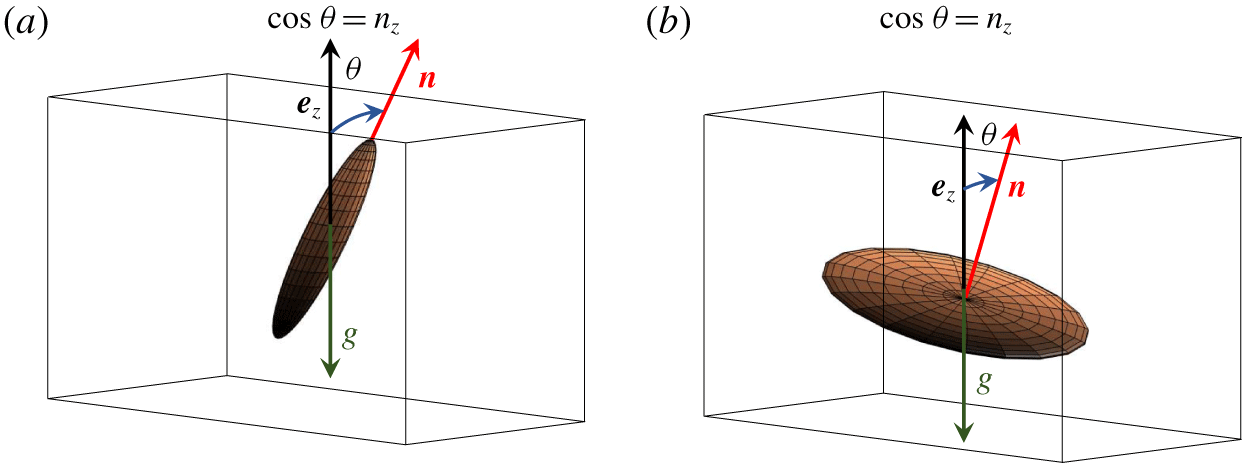
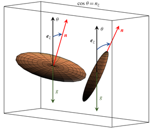
 $\boldsymbol{n}$ a unit vector aligned with the symmetry axis of the particle (figure 1). The motion of a solid particle is entirely characterised by the velocity of its centre of mass,
 $\boldsymbol{v}$, and its angular velocity,
 $\unicode[STIX]{x1D74E}$. In the following, we consider particles heavier than the fluid,
 $\unicode[STIX]{x1D70C}_{p}\gg \unicode[STIX]{x1D70C}_{f}$.
Definition of  $n_{z}$ (projection on the vertical axis of the unit vector aligned with the particle symmetry axis) for (a) prolate and (b) oblate particles.

We assume that the particles are sufficiently small compared to the size of the smallest eddies  $\unicode[STIX]{x1D702}$, the Kolmogorov length:
 $\tilde{a}<\unicode[STIX]{x1D702}$. To describe the dynamics of the settling particle in this limit, we use the same model as Klett (Reference Klett1995) and Lopez & Guazzelli (Reference Lopez and Guazzelli2017). This model can be rigorously justified only for a particle settling in a homogeneous flow at small particle Reynolds number
 $Re_{p}\equiv u_{s}\tilde{a}/\unicode[STIX]{x1D708}$, where
 $u_{s}$ is the slip velocity (Cox Reference Cox1965; Happel & Brenner Reference Happel and Brenner1983; Khayat & Cox Reference Khayat and Cox1989; Dabade et al. Reference Dabade, Marath and Subramanian2015), and neglecting the effects of shear and unsteadiness (Candelier, Einarsson & Mehlig Reference Candelier, Einarsson and Mehlig2016). But the model was shown to qualitatively describe the angular dynamics of rods settling in a 2-D vortex flow (Lopez & Guazzelli Reference Lopez and Guazzelli2017). In this model, the equation of motion describing the evolution of the particle velocity
 $\boldsymbol{v}(t)$ in the laboratory frame reads
 $$\begin{eqnarray}{\displaystyle \frac{\text{d}\boldsymbol{v}}{\text{d}t}}=\boldsymbol{g}+{\displaystyle \frac{6\unicode[STIX]{x03C0}\unicode[STIX]{x1D707}\tilde{a}}{m_{p}}}\unicode[STIX]{x1D648}_{St}\boldsymbol{\cdot }(\boldsymbol{u}-\boldsymbol{v})+{\displaystyle \frac{1}{m_{p}}}{\displaystyle \frac{9\unicode[STIX]{x03C0}}{8}}\unicode[STIX]{x1D70C}_{f}\tilde{a}^{2}|\boldsymbol{u}-\boldsymbol{v}|\unicode[STIX]{x1D648}_{I}\boldsymbol{\cdot }(\boldsymbol{u}-\boldsymbol{v}),\end{eqnarray}$$
where  $\boldsymbol{g}$ is gravity and
 $\boldsymbol{u}=\boldsymbol{u}(\boldsymbol{x}(t),t)$ represents the undisturbed velocity at the particle location,
 $\boldsymbol{x}(t)$, at time
 $t$. Aside from gravitational settling, the force acting on the particle results from the slip velocity,
 $\boldsymbol{u}_{s}=\boldsymbol{v}-\boldsymbol{u}$. Together with the equation
 $\text{d}\boldsymbol{x}/\text{d}t=\boldsymbol{v}$, equation (2.1) determines the position of the particle centre of mass. The second term on the right-hand side (r.h.s.) of (2.1) expresses the Stokes drag force, appropriate for a spheroidal particle. The expression of this force involves the anisotropic drag tensor
 $$\begin{eqnarray}\unicode[STIX]{x1D648}_{St}=X^{A}\boldsymbol{n}\boldsymbol{n}+Y^{A}(\mathbb{I}-\boldsymbol{n}\boldsymbol{n}),\end{eqnarray}$$
where  $\boldsymbol{n}$ is the unit vector defined above (see figure 1),
 $\mathbb{I}$ is the identity matrix, and
 $X^{A}$ and
 $Y^{A}$ are dimensionless coefficients that depend only on the shape of the spheroid through the parameter
 $\unicode[STIX]{x1D6FD}$. Their expressions are standard (Happel & Brenner Reference Happel and Brenner1983) and can be found in appendix A. The third term on the r.h.s. of (2.1) represents the inertial contribution to the force. The dimensionless tensor
 $\unicode[STIX]{x1D648}_{I}$ takes the form
 $$\begin{eqnarray}\unicode[STIX]{x1D648}_{I}=[3X^{A}-(X^{A}\cos ^{2}\unicode[STIX]{x1D6FC}+Y^{A}\sin ^{2}\unicode[STIX]{x1D6FC})]X^{A}\boldsymbol{n}\boldsymbol{n}+[3Y^{A}-(X^{A}\cos ^{2}\unicode[STIX]{x1D6FC}+Y^{A}\sin ^{2}\unicode[STIX]{x1D6FC})]Y^{A}(\mathbb{I}-\boldsymbol{n}\boldsymbol{n}),\end{eqnarray}$$
where  $\unicode[STIX]{x1D6FC}$ is the angle between the slip velocity
 $\boldsymbol{u}_{s}=\boldsymbol{v}-\boldsymbol{u}$ and
 $\boldsymbol{n}$ (
 $\unicode[STIX]{x1D6FC}=\cos ^{-1}(\boldsymbol{u}_{s}\boldsymbol{\cdot }\boldsymbol{n}/|\boldsymbol{u}_{s}|)$).
The angular equation of motion reads
 $$\begin{eqnarray}{\displaystyle \frac{\text{d}\hat{\unicode[STIX]{x1D74E}}}{\text{d}t}}=\left(\begin{array}{@{}c@{}}\hat{T}_{xx}/\hat{I} _{xx}\\ \hat{T}_{yy}/\hat{I} _{yy}\\ \hat{T}_{zz}/\hat{I} _{zz}\end{array}\right)+\left(\begin{array}{@{}c@{}}\hat{\unicode[STIX]{x1D714}}_{y}\hat{\unicode[STIX]{x1D714}}_{z}{\displaystyle \frac{\hat{I} _{yy}-\hat{I} _{zz}}{\hat{I} _{xx}}}\\ \hat{\unicode[STIX]{x1D714}}_{z}\hat{\unicode[STIX]{x1D714}}_{x}{\displaystyle \frac{\hat{I} _{zz}-\hat{I} _{xx}}{\hat{I} _{yy}}}\\ \hat{\unicode[STIX]{x1D714}}_{x}\hat{\unicode[STIX]{x1D714}}_{y}{\displaystyle \frac{\hat{I} _{xx}-\hat{I} _{yy}}{\hat{I} _{zz}}}\end{array}\right).\end{eqnarray}$$
Here we have expressed the equations of motion in the particle frame  $(\hat{x},{\hat{y}},\hat{z})$ with axes
 $\hat{\boldsymbol{e}}_{x}$,
 $\hat{\boldsymbol{e}}_{y}$,
 $\hat{\boldsymbol{e}}_{z}$ attached to the particle. Hereafter, all the quantities expressed in this frame carry a hat. The relation between a tensor expressed in the reference frame of the particle,
 $\hat{\unicode[STIX]{x1D646}}$, and in the reference frame of the laboratory,
 $\unicode[STIX]{x1D646}$, is given by
 $\hat{\unicode[STIX]{x1D646}}=\unicode[STIX]{x1D64D}^{rot}\unicode[STIX]{x1D646}\unicode[STIX]{x1D64D}^{rot^{-1}}$, where
 $\unicode[STIX]{x1D64D}^{rot}$ is the rotation matrix between the two frames. We note that the equation of evolution of
 $\unicode[STIX]{x1D64D}^{rot}$ is simply
 $\text{d}R_{ij}^{rot}/\text{d}t=\unicode[STIX]{x1D700}_{ikl}\unicode[STIX]{x1D714}_{k}R_{lj}^{rot}$, where
 $\unicode[STIX]{x1D700}_{ijk}$ is the Levi-Civita symbol. In our simulations, rotations were represented in terms of quaternions (Almondo et al. Reference Almondo, Einarsson, Angilella and Mehlig2018; Jucha et al. Reference Jucha, Naso, Lévêque and Pumir2018; Naso et al. Reference Naso, Jucha, Lévêque and Pumir2018). The tensor
 $\hat{\unicode[STIX]{x1D644}}$ is the moment-of-inertia tensor, which is diagonal in the reference frame of the particle
 $(\hat{x},{\hat{y}},\hat{z})$:
 $\hat{\unicode[STIX]{x1D644}}=(4\unicode[STIX]{x03C0}\unicode[STIX]{x1D70C}_{p}a^{5}\unicode[STIX]{x1D6FD}/15)\,\text{diag}(1+\unicode[STIX]{x1D6FD}^{2},1+\unicode[STIX]{x1D6FD}^{2},2)$. The second term on the r.h.s. of (2.4) represents the torque induced by the non-Galilean nature of the particle frame (Landau & Lifschitz Reference Landau and Lifschitz1976). The first term on the r.h.s. of (2.4) results from the hydrodynamic torque
 $\hat{\boldsymbol{T}}$ acting on the particle.
Following Lopez & Guazzelli (Reference Lopez and Guazzelli2017), we express  $\hat{\boldsymbol{T}}$ as the sum of Jeffery’s torque (Jeffery Reference Jeffery1922),
 $\hat{\boldsymbol{T}}_{St}$, and of the contribution due to fluid inertia (Cox Reference Cox1965; Khayat & Cox Reference Khayat and Cox1989; Dabade et al. Reference Dabade, Marath and Subramanian2015),
 $\hat{\boldsymbol{T}}_{I}$, for a particle moving steadily in a homogeneous flow:
 $\hat{\boldsymbol{T}}=\hat{\boldsymbol{T}}_{St}+\hat{\boldsymbol{T}}_{I}$. Jeffery’s torque is given by (Jeffery Reference Jeffery1922)
 $$\begin{eqnarray}\hat{\boldsymbol{T}}_{St}=\frac{16}{3}\unicode[STIX]{x03C0}\unicode[STIX]{x1D707}a^{3}\unicode[STIX]{x1D6FD}\left(\begin{array}{@{}ccc@{}}{\displaystyle \frac{1+\unicode[STIX]{x1D6FD}^{2}}{\unicode[STIX]{x1D6FC}_{0}+\unicode[STIX]{x1D6FD}^{2}\unicode[STIX]{x1D6FE}_{0}}} & 0 & 0\\ 0 & {\displaystyle \frac{1+\unicode[STIX]{x1D6FD}^{2}}{\unicode[STIX]{x1D6FC}_{0}+\unicode[STIX]{x1D6FD}^{2}\unicode[STIX]{x1D6FE}_{0}}} & 0\\ 0 & 0 & {\displaystyle \frac{1}{\unicode[STIX]{x1D6FC}_{0}}}\end{array}\right)\left(\begin{array}{@{}c@{}}{\displaystyle \frac{1-\unicode[STIX]{x1D6FD}^{2}}{1+\unicode[STIX]{x1D6FD}^{2}}}{\hat{S}}_{zy}+(\hat{\unicode[STIX]{x1D6FA}}_{zy}-\hat{\unicode[STIX]{x1D714}}_{x})\\[6.0pt] {\displaystyle \frac{\unicode[STIX]{x1D6FD}^{2}-1}{1+\unicode[STIX]{x1D6FD}^{2}}}{\hat{S}}_{xz}+(\hat{\unicode[STIX]{x1D6FA}}_{xz}-\hat{\unicode[STIX]{x1D714}}_{y})\\[6.0pt] \hat{\unicode[STIX]{x1D6FA}}_{yx}-\hat{\unicode[STIX]{x1D714}}_{z}\end{array}\right),\end{eqnarray}$$
where  ${\hat{S}}_{ij}$ and
 $\hat{\unicode[STIX]{x1D6FA}}_{i}$ are the components of the strain and vorticity, expressed in the reference frame of the particle. The quantities
 $\unicode[STIX]{x1D6FC}_{0}$ and
 $\unicode[STIX]{x1D6FE}_{0}$ are dimensionless, and depend only on
 $\unicode[STIX]{x1D6FD}$; see appendix A. The torque induced by convective fluid inertia, derived by Dabade et al. (Reference Dabade, Marath and Subramanian2015), reads (to order
 $Re_{p}$)
 $$\begin{eqnarray}\hat{\boldsymbol{T}}_{I}=\unicode[STIX]{x1D64D}^{rot}\boldsymbol{T}_{I},\quad \text{with}\quad \boldsymbol{T}_{I}=-\unicode[STIX]{x1D70C}_{f}|\boldsymbol{u}-\boldsymbol{v}|^{2}\tilde{a}^{3}F_{\unicode[STIX]{x1D6FD}}\left({\displaystyle \frac{\boldsymbol{u}_{s}}{|\boldsymbol{u}_{s}|}}\boldsymbol{\cdot }\boldsymbol{n}\right)\left({\displaystyle \frac{\boldsymbol{u}_{s}}{|\boldsymbol{u}_{s}|}}\times \boldsymbol{n}\right),\end{eqnarray}$$
where  $F_{\unicode[STIX]{x1D6FD}}$ is a dimensionless shape factor, which depends only on
 $\unicode[STIX]{x1D6FD}$. Its expression is given in appendix A. We have neglected here possible fluid-inertia corrections due to shear. This is justified provided that the Oseen length,
 $\ell _{O}\approx \unicode[STIX]{x1D708}/W_{s}$, is much smaller than the Saffman length,
 $\ell _{S}\approx (\unicode[STIX]{x1D708}/s)^{1/2}$, where
 $s$ is the order of magnitude of the velocity gradients in the flow (Candelier et al. Reference Candelier, Mehlig and Magnaudet2019). We must therefore require that
 $\ell _{S}/\ell _{O}\gg 1$, an assumption we reconsider in the following section.
3 Relative importance of Jeffery’s torque and fluid-inertia torque
3.1 General analysis
To estimate the relative importance of the inertial effects on the dynamics of the particles’ orientation, we calculate the ratio  $|\hat{\boldsymbol{T}}_{I}|/|\hat{\boldsymbol{T}}_{St}|$. The particles’ orientational dynamics is therefore expected to be correctly described by the Jeffery torque when this ratio is
 $\ll 1$. We begin by looking at the case of very slim, prolate spheroids, with
 $\unicode[STIX]{x1D6FD}\gg 1$. In this limit, one obtains
 $$\begin{eqnarray}\displaystyle & \displaystyle {\displaystyle \frac{\hat{T}_{I,x}}{\hat{T}_{St,x}}}\sim {\displaystyle \frac{\hat{T}_{I,y}}{\hat{T}_{St,y}}}\sim {\displaystyle \frac{5u_{s}^{2}}{8\unicode[STIX]{x1D708}s\log \unicode[STIX]{x1D6FD}}}, & \displaystyle\end{eqnarray}$$
 $$\begin{eqnarray}\displaystyle & \displaystyle {\displaystyle \frac{\hat{T}_{I,z}}{\hat{T}_{St,z}}}\sim {\displaystyle \frac{5u_{s}^{2}\unicode[STIX]{x1D6FD}^{2}}{16\unicode[STIX]{x1D708}s(\log \unicode[STIX]{x1D6FD})^{2}}}, & \displaystyle\end{eqnarray}$$
where we recall that  $\boldsymbol{u}_{s}$ is the slip velocity, and where
 $s$ is the inverse of a characteristic time scale representing the angular slip velocity
 $|\unicode[STIX]{x1D734}-\unicode[STIX]{x1D74E}|$ or the local strain
 $|\boldsymbol{S}|$. To estimate the ratio between
 $\hat{T}_{I}$ and
 $\hat{T}_{St}$ in (3.1) and (3.2), we used the fact that
 $F_{\unicode[STIX]{x1D6FD}}$ is no larger than
 $1$ for fibres with
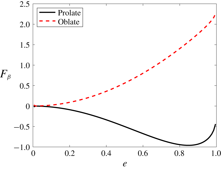
 $\unicode[STIX]{x1D6FD}\gg 1$; see figure 6. The terms responsible for the change in orientation are the
 $\hat{x}$ and
 ${\hat{y}}$ components in (3.1). For the present purpose, we therefore consider only these components. As we are interested only in orders of magnitude, we will approximate
 $5/8$ by
 $1$ in the following, and the
 $\log \unicode[STIX]{x1D6FD}$ factor, which in practice is close to
 $1$ if
 $5\leqslant \unicode[STIX]{x1D6FD}\leqslant 100$, will be omitted.
In the opposite limit of very thin disks,  $\unicode[STIX]{x1D6FD}\ll 1$, one obtains
 $$\begin{eqnarray}{\displaystyle \frac{\hat{T}_{I}}{\hat{T}_{St}}}\sim {\displaystyle \frac{3}{32}}F_{0}{\displaystyle \frac{u_{s}^{2}}{\unicode[STIX]{x1D708}s}},\end{eqnarray}$$
where  $u_{s}$ and
 $s$ are defined as before, and
 $F_{0}=\lim _{\unicode[STIX]{x1D6FD}\rightarrow 0}F_{\unicode[STIX]{x1D6FD}}=38/9-17\,216/(945\unicode[STIX]{x03C0}^{2})$ (Dabade et al. Reference Dabade, Marath and Subramanian2015), so
 $3F_{0}/32\sim 1$. The factor
 $F_{\unicode[STIX]{x1D6FD}}$ has once again been omitted since its absolute value is always smaller than
 $2.5$, as shown in figure 6. Equation (3.3) for disks therefore only differs from (3.1) for rods by the
 $1/\log \unicode[STIX]{x1D6FD}$ factor, which in practice does not vary much, as mentioned in the previous paragraph.
To summarise, for very flat disks ( $\unicode[STIX]{x1D6FD}\ll 1$) and for thin rods (
 $5\leqslant \unicode[STIX]{x1D6FD}\leqslant 100$, not too thin, so that the value of
 $\log \unicode[STIX]{x1D6FD}$ remains moderate), the ratio
 $\hat{T}_{I}/\hat{T}_{St}$ is of order
 ${\mathcal{R}}$, defined by
 $$\begin{eqnarray}|\boldsymbol{T}_{I}|/|\boldsymbol{T}_{St}|\sim {\mathcal{R}}\quad \text{with}\quad {\mathcal{R}}\equiv {\displaystyle \frac{|\boldsymbol{u}-\boldsymbol{v}|^{2}}{\unicode[STIX]{x1D708}|\unicode[STIX]{x1D734}-\unicode[STIX]{x1D74E}|}},\end{eqnarray}$$
where  $\boldsymbol{v}$ is the particle velocity,
 $\unicode[STIX]{x1D74E}$ is its angular velocity,
 $\boldsymbol{u}$ is the fluid velocity,
 $\unicode[STIX]{x1D734}$ is half the vorticity and
 $\unicode[STIX]{x1D708}$ is the viscosity of the fluid. The differences
 $|\boldsymbol{u}-\boldsymbol{v}|$ and
 $|\unicode[STIX]{x1D734}-\unicode[STIX]{x1D74E}|$ are the translational and rotational slip velocities. The convective fluid inertia torque dominates when
 ${\mathcal{R}}\gg 1$; in this case a spheroid settles with maximal drag. When
 ${\mathcal{R}}\ll 1$, by contrast, we expect a spheroid to settle with minimal drag. To provide an estimate for
 ${\mathcal{R}}$, we approximate the slip velocity as
 $u_{s}\sim W_{s}$, where
 $W_{s}\approx g\unicode[STIX]{x1D70F}_{p}$ is the settling velocity of the particle. Here
 $\unicode[STIX]{x1D70F}_{p}$ is an estimate of its response time, defined as
 $a^{2}\log \unicode[STIX]{x1D6FD}\,(\unicode[STIX]{x1D70C}_{p}/\unicode[STIX]{x1D70C}_{f})/(3\unicode[STIX]{x1D708})$ for prolate bodies and
 $\unicode[STIX]{x03C0}a^{2}\unicode[STIX]{x1D6FD}(\unicode[STIX]{x1D70C}_{p}/\unicode[STIX]{x1D70C}_{f})/(8\unicode[STIX]{x1D708})$ for oblate ones (strictly speaking, the particle linear response time depends on its orientation, as stated in (2.1)). To estimate the inverse characteristic time scale
 $s$, we need to distinguish the laminar and turbulent cases.
3.2 Turbulent flows
Turbulent flows generate large gradients. Standard estimates show that the vorticity root-mean square is of order  $|\langle \unicode[STIX]{x1D734}^{2}\rangle ^{1/2}|\sim (U_{0}/L)Re_{f}^{1/2}$. Substituting this expression together with
 $|\boldsymbol{u}-\boldsymbol{v}|\sim W_{s}$ in (3.4), leads to
 $$\begin{eqnarray}{\mathcal{R}}\sim \left({\displaystyle \frac{W_{s}}{U_{0}}}\right)^{2}Re_{f}^{1/2}\,.\end{eqnarray}$$
Using the Kolmogorov velocity scale (Frisch Reference Frisch1995),  $u_{K}\sim U_{0}Re_{f}^{-1/4}$, we can rewrite this estimate as
 ${\mathcal{R}}\sim (W_{s}/u_{K})^{2}$, consistent with the formulation in Gustavsson et al. (Reference Gustavsson, Sheikh, Lopez, Naso, Pumir and Mehlig2019), where the width of the orientation distribution in the limit
 ${\mathcal{R}}\gg 1$ is evaluated. In any case, equation (3.5) shows that, in the high-
 $Re_{f}$ regime, the fluid-inertia torque can be neglected (i.e.
 ${\mathcal{R}}$ can be small) only if
 $W_{s}/U_{0}$ is small. In this limit, the orientation distribution is approximately uniform, as shown in Siewert et al. (Reference Siewert, Kunnen, Meinke and Schröder2014a,Reference Siewert, Kunnen and Schröderb), Gustavsson et al. (Reference Gustavsson, Jucha, Naso, Lévêque, Pumir and Mehlig2017) and Jucha et al. (Reference Jucha, Naso, Lévêque and Pumir2018). This means that the orientation bias analysed in these works (preferential minimal drag) cannot be actually observed at large
 $Re_{f}$.
The estimate for the velocity gradients,  $s\sim 1/\unicode[STIX]{x1D70F}_{K}$, leads to the ratio between the Saffman and the Oseen lengths (Candelier et al. Reference Candelier, Mehlig and Magnaudet2019),
 $\ell _{S}/\ell _{O}\sim {\mathcal{R}}^{1/2}\sim W_{s}/u_{K}$. This demonstrates that neglecting fluid-inertia effects due to shear, as done here, is consistent when
 ${\mathcal{R}}\gg 1$.
3.3 Laminar flows
The analysis developed in § 3.1 applies also to a laminar flow, such as the cellular flow considered by Lopez & Guazzelli (Reference Lopez and Guazzelli2017). In the case of a laminar flow, at small  $Re_{f}$, the velocity gradient can be simply estimated as
 $s\sim U_{0}/L$, so that (3.4) yields
 $$\begin{eqnarray}{\mathcal{R}}\sim \left({\displaystyle \frac{W_{s}}{U_{0}}}\right)^{2}Re_{f}.\end{eqnarray}$$
We remark that the relative magnitude of the fluid-inertia contributions to the angular dynamics (appendix B of Lopez & Guazzelli (Reference Lopez and Guazzelli2017)) amounts to  $Re_{p}w_{0}/\unicode[STIX]{x1D706}_{p}$, where
 $Re_{p}=\unicode[STIX]{x1D6FD}aW_{s}/\unicode[STIX]{x1D708}$,
 $w_{0}=W_{s}/U_{0}$ and
 $\unicode[STIX]{x1D706}_{p}=\unicode[STIX]{x1D6FD}a/L$. As a result, our expression (3.6) coincides with theirs. Equation (3.6) suggests that the distribution of orientation predicted in Siewert et al. (Reference Siewert, Kunnen, Meinke and Schröder2014a,Reference Siewert, Kunnen and Schröderb), Gustavsson et al. (Reference Gustavsson, Jucha, Naso, Lévêque, Pumir and Mehlig2017), Jucha et al. (Reference Jucha, Naso, Lévêque and Pumir2018) and Naso et al. (Reference Naso, Jucha, Lévêque and Pumir2018) – spheroids settling preferentially with minimal drag, corresponding to
 ${\mathcal{R}}<1$ and
 $W_{s}/U_{0}>1$ – could be observable at small
 $Re_{f}$.
We note that estimating  ${\mathcal{R}}$ in the limit
 $Re_{f}\rightarrow 0$ requires some care. To fully analyse the problem, it is convenient to introduce, in addition to
 $U_{0}$ and
 $W_{s}$, the velocity
 $V_{\unicode[STIX]{x1D708}}=\unicode[STIX]{x1D708}/L$, where
 $L$ is the characteristic length scale of the problem and
 $\unicode[STIX]{x1D708}$ is the viscosity. The two dimensionless parameters
 $Re_{f}$ and
 ${\mathcal{R}}$ can simply be expressed as
 $Re_{f}=U_{0}/V_{\unicode[STIX]{x1D708}}$ and
 ${\mathcal{R}}=(W_{s}/U_{0})(W_{s}/V_{\unicode[STIX]{x1D708}})$. The limit
 $Re_{f}\rightarrow 0$ may be reached in two very different ways, by letting either
 $U_{0}\rightarrow 0$ or
 $V_{\unicode[STIX]{x1D708}}\rightarrow \infty$. In the former case,
 $U_{0}\rightarrow 0$ at fixed
 $V_{\unicode[STIX]{x1D708}}$, the parameter
 ${\mathcal{R}}$ is very large, so the fluid inertia dominates. In contrast, letting
 $V_{\unicode[STIX]{x1D708}}\rightarrow \infty$ at fixed
 $U_{0}$ leads to
 ${\mathcal{R}}\rightarrow 0$, so the Jeffery torque prevails. A careful estimate of the ratios between
 $W_{s}$,
 $U_{0}$ and
 $V_{\unicode[STIX]{x1D708}}$ is therefore necessary to come to a conclusion about the importance of fluid inertia in the
 $Re_{f}\rightarrow 0$ limit.
To summarise, the main result of this section is our systematic analysis of the ratio between the torque induced by fluid convection and the Jeffery torque, and quantified by  ${\mathcal{R}}$, introduced by (3.4). With our definition, the torque induced by convective forces dominates when
 ${\mathcal{R}}\gg 1$. A more refined relation between
 ${\mathcal{R}}$, the Reynolds number
 $Re_{f}$, and the ratio between the settling velocity
 $W_{s}$ and the flow velocity
 $U_{0}$ depends on whether the flow is turbulent, equation (3.5), or laminar, equation (3.6).
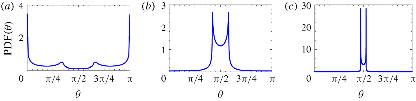
Distribution of  $\unicode[STIX]{x1D703}$ (angle between the axis of symmetry of the particle and gravity) for prolate bodies of aspect ratio
 $\unicode[STIX]{x1D6FD}=20$ in the 2-D vortex flow: (a)
 ${\mathcal{R}}=10^{-3}$ (
 $W_{s}/U_{0}\approx 0.283$,
 $Re_{f}=1/80$), (b)
 ${\mathcal{R}}=0.1$ (
 $W_{s}/U_{0}\approx 2.88$,
 $Re_{f}=1/80$) and (c)
 ${\mathcal{R}}=4.0$ (
 $W_{s}/U_{0}\approx 6.32$,
 $Re_{f}=0.1$). A uniform distribution of
 $\unicode[STIX]{x1D703}$ would correspond to a random orientation of the particle.

4 Results of numerical simulations
In this section, we test numerically the results of the analysis of the previous section. To this end, we study the dynamics of spheroids in a model flow that describes low- $Re_{f}$ flows, as well as high-
 $Re_{f}$ (turbulent) flows with many spatial scales.
4.1 Two-dimensional vortex flow
We performed numerical simulations of prolate spheroids ( $\unicode[STIX]{x1D6FD}=20$) settling in a simple 2-D cellular flow mimicking that of Lopez & Guazzelli (Reference Lopez and Guazzelli2017). The (marginal) probability distribution function of
 $\unicode[STIX]{x1D703}$, the angle between the axis of symmetry of the particle and gravity, is shown in figure 2 for different values of
 ${\mathcal{R}}$. In this 2-D flow, a random orientation of the particle would result in a uniform distribution of
 $\unicode[STIX]{x1D703}$. The distributions shown in figure 2 are symmetric with respect to the value
 $\unicode[STIX]{x03C0}/2$, as expected due to the symmetry of the objects. At low values of
 ${\mathcal{R}}$ (figure 2a), the orientation distribution exhibits peaks around
 $\unicode[STIX]{x1D703}\approx 0$ and
 $\unicode[STIX]{x1D703}\approx \unicode[STIX]{x03C0}$. Here
 $\unicode[STIX]{x1D703}$ is the angle between
 $\boldsymbol{n}$ and the direction of gravity (figure 1), so this corresponds to rods settling with their tips first. As the value of
 ${\mathcal{R}}$ increases (figure 2b,c), however, the peaks migrate towards
 $\unicode[STIX]{x1D703}\approx \unicode[STIX]{x03C0}/2$. This corresponds to rods settling with their broad sides first.
4.2 Three-dimensional turbulence
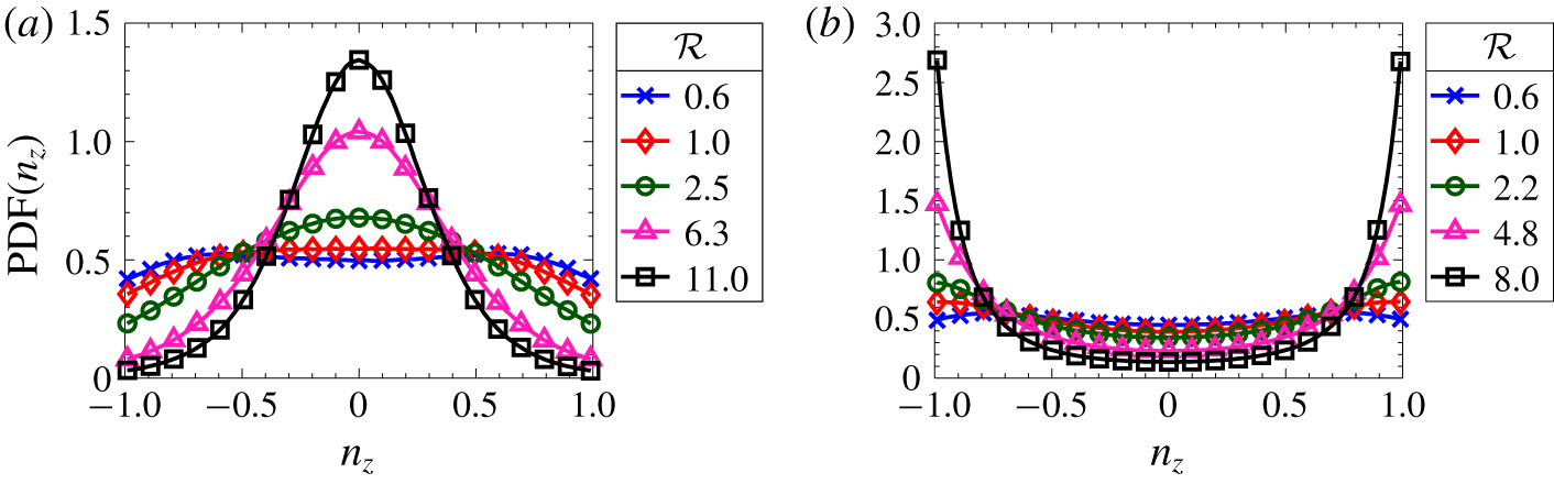
Distribution of  $n_{z}$ for (a) prolate (
 $\unicode[STIX]{x1D6FD}=5$) and (b) oblate (
 $\unicode[STIX]{x1D6FD}=0.02$) particles in the 3-D turbulent flow (DNS), for
 $St=0.1$ and several values of
 ${\mathcal{R}}$. In this 3-D flow, a random orientation of the particles would be reflected by a uniform distribution of
 $n_{z}$.

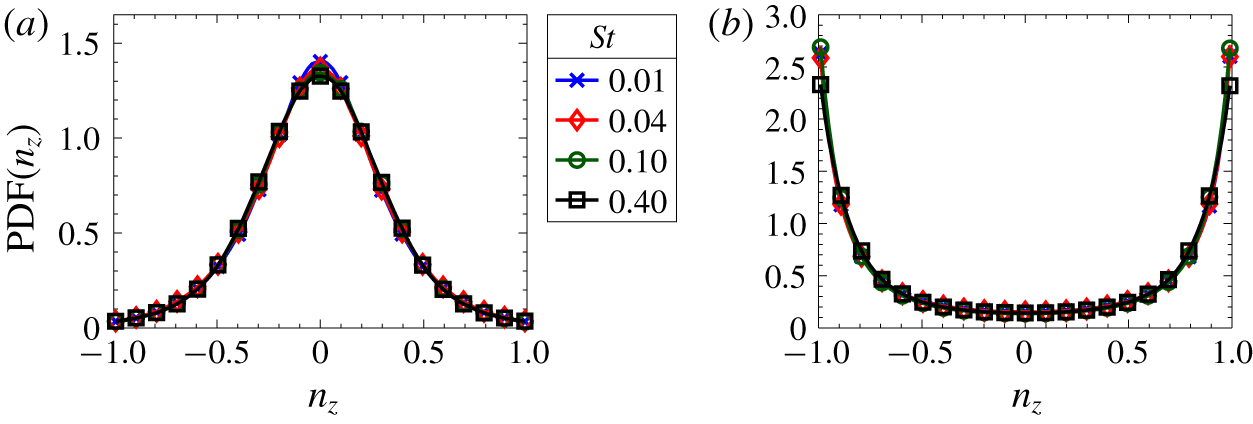
Distribution of  $n_{z}$ for
 ${\mathcal{R}}\approx 10$ and several values of the Stokes number, for (a) prolate (
 $\unicode[STIX]{x1D6FD}=5$) and (b) oblate (
 $\unicode[STIX]{x1D6FD}=0.02$) particles in the 3-D turbulent flow.

We investigate turbulent flows in a cubical box with periodic boundary conditions in all directions. Our pseudo-spectral code (see e.g. Jucha et al. Reference Jucha, Naso, Lévêque and Pumir2018) is fully dealiased. We used a grid resolution  $N^{3}=128^{3}$, corresponding to a Reynolds number based on the Taylor microscale
 $R_{\unicode[STIX]{x1D706}}=40$. An external force acts on low-wavenumber modes to ensure a constant injection rate of energy,
 $\unicode[STIX]{x1D700}=100~\text{cm}^{2}~\text{s}^{-3}$, and reach stationary homogeneous and isotropic turbulence. The kinematic viscosity
 $\unicode[STIX]{x1D708}=0.15~\text{cm}^{2}~\text{s}^{-1}$ has been adjusted to get a satisfactory grid resolution
 $k_{max}\unicode[STIX]{x1D702}\sim 3.4$, where
 $k_{max}$ is the highest wavenumber and
 $\unicode[STIX]{x1D702}=(\unicode[STIX]{x1D708}^{3}/\unicode[STIX]{x1D700})^{1/4}$ is the Kolmogorov scale.
Figures 3 and 4 display the results of our simulations. Shown is the distribution of  $n_{z}$, the projection on the vertical axis of the unit vector aligned with the particle symmetry axis (see figure 1). In three-dimensional (3-D) flows, such a distribution would be uniform if the spheroids were randomly oriented. The distribution of
 $n_{z}$ is first shown for different values of
 ${\mathcal{R}}$, for prolate spheroids (
 $\unicode[STIX]{x1D6FD}=5$) in figure 3(a) and for oblate spheroids (
 $\unicode[STIX]{x1D6FD}=0.02$) in figure 3(b). These results were obtained for a constant value of the Stokes number
 $St=\unicode[STIX]{x1D70F}_{p}/\unicode[STIX]{x1D70F}_{K}$, where
 $\unicode[STIX]{x1D70F}_{K}$ is the Kolmogorov time scale.
As expected, figure 3 shows that for  ${\mathcal{R}}\lesssim 1$ the distribution of angles is almost uniform. When the parameter
 ${\mathcal{R}}$ becomes larger than
 $1$, the fluid-inertia torque dominates the angular dynamics. For prolate particles (figure 3a) the distribution peaks at
 $n_{z}\approx 0$, so that
 $\boldsymbol{n}\bot \boldsymbol{g}$. This corresponds to particles settling with their long side first. For oblate spheroids, on the other hand (figure 3b), the distributions peak at
 $n_{z}=\pm 1$. This corresponds to disks settling with their broad sides first. For increasing values of
 ${\mathcal{R}}$ (not shown here), the distributions of
 $n_{z}$ become more and more peaked around
 $n_{z}=0$ for prolate spheroids, and at
 $n_{z}=\pm 1$ for oblate particles.
Our simulation results fully support the prediction that, when the settling parameter  $w_{0}=W_{s}/U_{0}$ is of order unity or larger, then
 ${\mathcal{R}}>1$ in a turbulent flow with large
 $Re_{f}$. In this case the fluid-inertia torque dominates the angular dynamics, leading to a distribution of orientation maximising the drag, at odds with the predictions of models neglecting this torque (Siewert et al. Reference Siewert, Kunnen, Meinke and Schröder2014a,Reference Siewert, Kunnen and Schröderb; Gustavsson et al. Reference Gustavsson, Jucha, Naso, Lévêque, Pumir and Mehlig2017; Jucha et al. Reference Jucha, Naso, Lévêque and Pumir2018; Naso et al. Reference Naso, Jucha, Lévêque and Pumir2018). A theory for the orientation distribution for
 ${\mathcal{R}}>1$, when the fluid-inertia torque dominates, has been derived by Gustavsson et al. (Reference Gustavsson, Sheikh, Lopez, Naso, Pumir and Mehlig2019); see also Kramel (Reference Kramel2017).
Figure 4 shows that, at a fixed value of  ${\mathcal{R}}$, the Stokes number has only a limited effect on the orientation statistics, for the range of parameters considered here (
 $St\lesssim 1$), consistent with the findings of Gustavsson et al. (Reference Gustavsson, Sheikh, Lopez, Naso, Pumir and Mehlig2019) (our numerical data exhibit the same behaviour for any value of
 ${\mathcal{R}}$).
Tables 1 and 2 list the parameters used in the simulations of figure 3 and 4, respectively. We defined the settling numbers  $Sv_{L}=g\unicode[STIX]{x1D70F}_{p}/U_{0}$ and
 $Sv_{\unicode[STIX]{x1D702}}=g\unicode[STIX]{x1D70F}_{p}/u_{K}$ and the velocity ratio
 $w_{0}=W_{s}/U_{0}$. The particle Reynolds number,
 $Re_{p}$, is defined as
 $W_{s}\tilde{a}/\unicode[STIX]{x1D708}$. The parameter
 $S=|\boldsymbol{u}-\boldsymbol{v}|/W_{s}$ is the ratio between the slip velocity and the settling velocity. Its value is always close to one, thereby confirming the fact that
 $|\boldsymbol{u}-\boldsymbol{v}|$ is, in the present set-up, always well approximated by
 $W_{s}$.


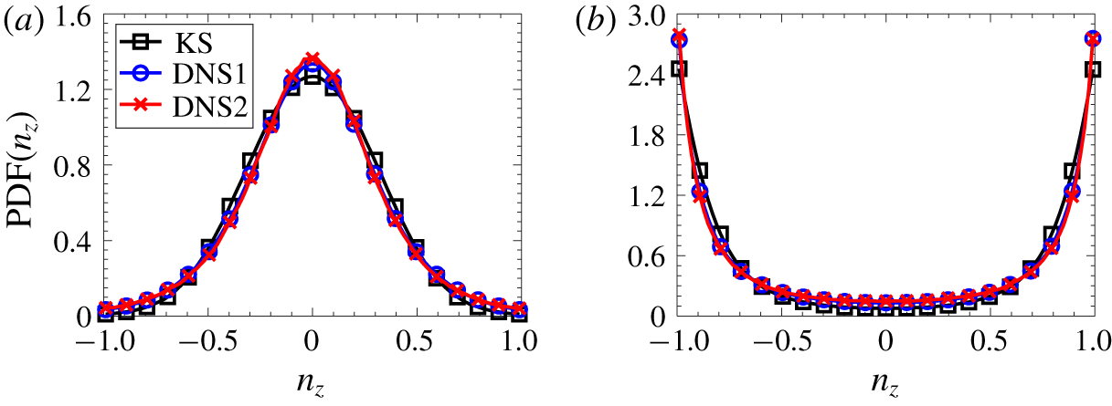
The previous results were obtained for a moderate value of  $R_{\unicode[STIX]{x1D706}}=40$. As shown in figure 5, similar results are obtained for
 $R_{\unicode[STIX]{x1D706}}=80$. Finally, we stress the fact that, for these very dense particles, similar results can also be obtained by using much more simplified models of turbulent flows. In fact, we compared directly the prediction of the kinematic simulation (KS) model of turbulence with the results of DNS. Briefly, the KS flow (Fung et al. Reference Fung, Hunt, Malik and Perkins1992) is obtained by representing the large range of scales in the flow by a superposition of a few Fourier modes, with a distribution of wavenumber amplitude in
 $k$-space. Details about our implementation can be found in Ducasse & Pumir (Reference Ducasse and Pumir2010). As shown in figure 5, we found a very good agreement between the DNS and KS results, as was the case in Gustavsson et al. (Reference Gustavsson, Jucha, Naso, Lévêque, Pumir and Mehlig2017). This can be understood by noting that the velocity gradient tensor acting on a settling particle decorrelates faster than on a tracer particle, and, as a result, the particle response is not sensitive to the fine correlations of the velocity gradient. The very good agreement between KS and DNS (not shown here) persists even at lower particle settling velocity, or equivalently at lower
 ${\mathcal{R}}$. Lowering the settling velocity makes the orientation distribution of the particle with respect to gravity closer to uniform, for both KS and DNS. Whereas the differences in the statistical properties of the velocity gradient tensor between KS and DNS affect the orientation of the particles with respect to the strain eigenvectors (Pumir & Wilkinson Reference Pumir and Wilkinson2011), or the tumbling rate of tracer particles (Shin & Koch Reference Shin and Koch2005; Parsa et al. Reference Parsa, Calzavarini, Toschi and Voth2012; Chevillard & Meneveau Reference Chevillard and Meneveau2013; Byron et al. Reference Byron, Einarsson, Gustavsson, Voth, Mehlig and Variano2015), they do not appear to play a major role for the distribution of orientation with respect to the direction of gravity.
Comparison of distribution of  $n_{z}$ calculated by KS and two runs of DNS,
 ${\mathcal{R}}\approx 10$ and
 $St=0.1$: (a) prolate (
 $\unicode[STIX]{x1D6FD}=5$) and (b) oblate (
 $\unicode[STIX]{x1D6FD}=0.02$) particles. DNS1 and KS, for
 $R_{\unicode[STIX]{x1D706}}=40$; DNS2, for
 $R_{\unicode[STIX]{x1D706}}=80$.

5 Discussion
The analysis and the numerical results presented here show that the effect of convective fluid inertia on the orientation of particles settling in a flow becomes important when the parameter  ${\mathcal{R}}$, defined by (3.4), is larger than unity. This condition implies that
 $(W_{s}/U_{0})^{2}Re_{f}^{\unicode[STIX]{x1D6FC}}\gtrsim 1$, where
 $\unicode[STIX]{x1D6FC}=1$ in the laminar regime (
 $Re_{f}<1$) and
 $\unicode[STIX]{x1D6FC}=1/2$ in the turbulent regime, at large Reynolds numbers.
For a turbulent flow, this condition implies that the effect of convective fluid inertia can only be neglected when  $W_{s}/U_{0}\ll 1$. In this limit, the orientation distribution is essentially uniform. When the ratio
 $W_{s}/U_{0}$ becomes of order unity, our study suggests that a particle tends to settle preferentially broad side down (maximising the drag). This conclusion has been previously reached by considering the restoring torque induced by convective inertia (Klett Reference Klett1995), and has also been observed in laboratory experiments (Kramel Reference Kramel2017). The expression for
 ${\mathcal{R}}$ given by (3.4) was derived in the limits of infinitely thin (
 $\unicode[STIX]{x1D6FD}\gg 1$) or infinitely flat (
 $\unicode[STIX]{x1D6FD}\ll 1$) particles, but our numerical results show that this parameter is also relevant for moderate values of
 $\unicode[STIX]{x1D6FD}$.
The present analysis was performed keeping, in addition to the Jeffery torque, only the leading- $Re_{p}$ contribution of the convective fluid-inertia torque for a particle settling slowly and steadily in a fluid at rest. This model has been validated, to some extent, in recent experimental work (Lopez & Guazzelli Reference Lopez and Guazzelli2017). This opens the possibility to quantitatively understand the orientation distribution of small non-spherical particles settling in turbulent flows (Gustavsson et al. Reference Gustavsson, Sheikh, Lopez, Naso, Pumir and Mehlig2019), a question of fundamental importance in cloud physics (Pruppacher & Klett Reference Pruppacher and Klett1997).
Acknowledgements
We acknowledge discussions with E. Guazzelli and J. Magnaudet. This work was supported by the IDEXLYON project (contract ANR-16-IDEX-0005) under University of Lyon auspices. We also acknowledge support from Vetenskapsrådet (grant number 2017-3865), from Formas (grant number 2014-585) and from the Knut and Alice Wallenberg Foundation (grant ‘Bottlenecks for particle growth in turbulent aerosols’ 2014.0048). The simulations were performed using the resources provided by PSMN (ENS Lyon).
Declaration of interests
The authors report no conflict of interest.
Appendix A. Expression of the coefficients  $X^{A}$, $Y^{A}$, $\unicode[STIX]{x1D6FC}_{0}$, $\unicode[STIX]{x1D6FE}_{0}$ and $F_{\unicode[STIX]{x1D6FD}}$


In the following, we introduce the ellipticity  $e$, defined for oblate bodies (
 $\unicode[STIX]{x1D6FD}<1$) by
 $e=\sqrt{1-\unicode[STIX]{x1D6FD}^{2}}$ and for prolate ones (
 $\unicode[STIX]{x1D6FD}>1$) by
 $e=\sqrt{1-(1/\unicode[STIX]{x1D6FD})^{2}}$.
Expression of the force We begin by giving the expressions of the coefficients  $X^{A}$ and
 $Y^{A}$ that define the tensors
 $\unicode[STIX]{x1D648}_{St}$ and
 $\unicode[STIX]{x1D648}_{I}$, introduced in (2.2) and (2.3). The expressions determined in Kim & Karrila (Reference Kim and Karrila1991) read as follows.
For prolate ellipsoids ( $\unicode[STIX]{x1D6FD}>1$):
 $$\begin{eqnarray}X^{A}={\displaystyle \frac{8e^{3}}{3\left(-2e+(1+e^{2})\ln \left({\displaystyle \frac{1+e}{1-e}}\right)\right)}},\quad Y^{A}={\displaystyle \frac{16e^{3}}{3\left(2e+(-1+3e^{2})\ln \left({\displaystyle \frac{1+e}{1-e}}\right)\right)}}.\end{eqnarray}$$
For oblate spheroids ( $\unicode[STIX]{x1D6FD}<1$):
 $$\begin{eqnarray}\displaystyle & \displaystyle X^{A}={\displaystyle \frac{4e^{3}}{3\left((2e^{2}-1)\cot ^{-1}\left({\displaystyle \frac{\sqrt{1-e^{2}}}{e}}\right)+e\sqrt{1-e^{2}}\right)}}, & \displaystyle\end{eqnarray}$$
 $$\begin{eqnarray}\displaystyle & \displaystyle Y^{A}={\displaystyle \frac{8e^{3}}{3\left((2e^{2}+1)\cot ^{-1}\left({\displaystyle \frac{\sqrt{1-e^{2}}}{e}}\right)-e\sqrt{1-e^{2}}\right)}}. & \displaystyle\end{eqnarray}$$
Expression of the torque The tensor necessary to calculate the Jeffery torque, see (2.5), requires the two parameters  $\unicode[STIX]{x1D6FC}_{0}$ and
 $\unicode[STIX]{x1D6FE}_{0}$ (Jeffery Reference Jeffery1922). Additionally, the expression for the torque due to inertial effects involves a factor
 $F_{\unicode[STIX]{x1D6FD}}$ (see (2.6)), derived by Dabade et al. (Reference Dabade, Marath and Subramanian2015) (equations (4.1) and (4.2) therein). The expressions of these parameters are given below, and the
 $\unicode[STIX]{x1D6FD}$ dependence of
 $F_{\unicode[STIX]{x1D6FD}}$ is more specifically shown in figure 6.
For prolate spheroids ( $\unicode[STIX]{x1D6FD}>1$):
 $$\begin{eqnarray}\unicode[STIX]{x1D6FC}_{0}={\displaystyle \frac{\unicode[STIX]{x1D6FD}^{2}}{\unicode[STIX]{x1D6FD}^{2}-1}}-{\displaystyle \frac{\text{arccosh}(\unicode[STIX]{x1D6FD})\unicode[STIX]{x1D6FD}}{(\unicode[STIX]{x1D6FD}^{2}-1)^{3/2}}},\quad \unicode[STIX]{x1D6FE}_{0}={\displaystyle \frac{-2}{\unicode[STIX]{x1D6FD}^{2}-1}}+{\displaystyle \frac{2\text{arccosh}(\unicode[STIX]{x1D6FD})\unicode[STIX]{x1D6FD}}{(\unicode[STIX]{x1D6FD}^{2}-1)^{3/2}}},\end{eqnarray}$$
 $$\begin{eqnarray}\displaystyle F_{\unicode[STIX]{x1D6FD}} & = & \displaystyle {\displaystyle \frac{-\unicode[STIX]{x03C0}e^{2}(420e+2240e^{3}+4249e^{5}-2152e^{7})}{315((e^{2}+1)\tanh ^{-1}e-e)^{2}((1-3e^{2})\tanh ^{-1}e-e)}}\nonumber\\ \displaystyle & & \displaystyle +\,{\displaystyle \frac{\unicode[STIX]{x03C0}e^{2}(420+3360e^{2}+1890e^{4}-1470e^{6})\tanh ^{-1}e}{315((e^{2}+1)\tanh ^{-1}e-e)^{2}((1-3e^{2})\tanh ^{-1}e-e)}}\nonumber\\ \displaystyle & & \displaystyle -\,{\displaystyle \frac{\unicode[STIX]{x03C0}e^{2}(1260e-1995e^{3}+2730e^{5}-1995e^{7})(\tanh ^{-1}e)^{2}}{315((e^{2}+1)\tanh ^{-1}e-e)^{2}((1-3e^{2})\tanh ^{-1}e-e)}}.\end{eqnarray}$$
For oblate spheroids ( $\unicode[STIX]{x1D6FD}<1$):
 $$\begin{eqnarray}\unicode[STIX]{x1D6FC}_{0}={\displaystyle \frac{\unicode[STIX]{x1D6FD}^{2}}{\unicode[STIX]{x1D6FD}^{2}-1}}+{\displaystyle \frac{\arccos (\unicode[STIX]{x1D6FD})\unicode[STIX]{x1D6FD}}{(1-\unicode[STIX]{x1D6FD}^{2})^{3/2}}},\quad \unicode[STIX]{x1D6FE}_{0}={\displaystyle \frac{2}{1-\unicode[STIX]{x1D6FD}^{2}}}-{\displaystyle \frac{2\arccos (\unicode[STIX]{x1D6FD})\unicode[STIX]{x1D6FD}}{(1-\unicode[STIX]{x1D6FD}^{2})^{3/2}}},\end{eqnarray}$$
 $$\begin{eqnarray}\displaystyle F_{\unicode[STIX]{x1D6FD}} & = & \displaystyle {\displaystyle \frac{\unicode[STIX]{x03C0}e^{3}\sqrt{1-e^{2}}(-420+3500e^{2}-9989e^{4}+4757e^{6})}{315\sqrt{1-e^{2}}(-e\sqrt{1-e^{2}}+(1+2e^{2})\sin ^{-1}e)(e\sqrt{1-e^{2}}+(2e^{2}-1)\sin ^{-1}e)^{2}}}\nonumber\\ \displaystyle & & \displaystyle +\,{\displaystyle \frac{210\unicode[STIX]{x03C0}e^{2}(2-24e^{2}+69e^{4}-67e^{6}+20e^{8})\sin ^{-1}e}{315\sqrt{1-e^{2}}(-e\sqrt{1-e^{2}}+(1+2e^{2})\sin ^{-1}e)(e\sqrt{1-e^{2}}+(2e^{2}-1)\sin ^{-1}e)^{2}}}\nonumber\\ \displaystyle & & \displaystyle +\,{\displaystyle \frac{105\unicode[STIX]{x03C0}e^{3}(12-17e^{2}+24e^{4})(\sin ^{-1}e)^{2}}{315(-e\sqrt{1-e^{2}}+(1+2e^{2})\sin ^{-1}e)(e\sqrt{1-e^{2}}+(2e^{2}-1)\sin ^{-1}e)^{2}}}.\end{eqnarray}$$
Parameter  $F_{\unicode[STIX]{x1D6FD}}$ plotted as a function of the particle ellipticity, for prolate and oblate spheroids.