2. Past theoretical modelling

2.1. The filling box model of Cooper & Hunt

The theoretical model of Cooper & Hunt (Reference Cooper and Hunt2010) describes a turbulent wall plume with a vertically distributed source of buoyancy. They use an approach that is similar to that of Morton, Taylor & Turner (Reference Morton, Taylor and Turner1956) for point sources of buoyancy. The model assumes top-hat profiles of all plume quantities and is based on a symmetric line plume. It does not include any viscous effects and predicts a velocity maximum immediately next to the wall. The height of the laminar portion of the boundary layer is also assumed to be negligible.

The model predicts that, for a turbulent wall plume in a uniform ambient fluid, the following relationships exist for the plume buoyancy flux,  $F$ , top-hat width,  $b_{P}$ , vertical velocity,  $w_{P}$ , buoyancy,  ${\it\Delta}_{P}$ , volume flux,  $Q_{P}$ , and momentum flux,  $M_{P}$ :

(2.1) $$\begin{eqnarray}\displaystyle & \displaystyle F={\it\Phi}z, & \displaystyle\end{eqnarray}$$

(2.2) $$\begin{eqnarray}\displaystyle & \displaystyle b_{P}={\textstyle \frac{3}{4}}{\it\alpha}_{P}z=C_{1}z, & \displaystyle\end{eqnarray}$$

(2.3) $$\begin{eqnarray}\displaystyle & \displaystyle w_{P}=\left({\textstyle \frac{4}{5}}\right)^{1/3}{\it\alpha}_{P}^{-1/3}{\it\Phi}^{1/3}z^{1/3}=C_{2}{\it\Phi}^{1/3}z^{1/3}, & \displaystyle\end{eqnarray}$$

(2.4) $$\begin{eqnarray}\displaystyle & \displaystyle {\it\Delta}_{P}={\textstyle \frac{4}{3}}\left({\textstyle \frac{5}{4}}\right)^{1/3}{\it\alpha}_{P}^{-2/3}{\it\Phi}^{2/3}z^{-1/3}=C_{3}{\it\Phi}^{2/3}z^{-1/3}, & \displaystyle\end{eqnarray}$$

(2.5) $$\begin{eqnarray}\displaystyle & \displaystyle Q_{P}={\textstyle \frac{3}{4}}\left({\textstyle \frac{4}{5}}\right)^{1/3}{\it\alpha}_{P}^{2/3}{\it\Phi}^{1/3}z^{4/3}=C_{4}{\it\Phi}^{1/3}z^{4/3}, & \displaystyle\end{eqnarray}$$

(2.6) $$\begin{eqnarray}\displaystyle & \displaystyle M_{P}={\textstyle \frac{3}{4}}\left({\textstyle \frac{4}{5}}\right)^{2/3}{\it\alpha}_{P}^{1/3}{\it\Phi}^{2/3}z^{5/3}=C_{5}{\it\Phi}^{2/3}z^{5/3}, & \displaystyle\end{eqnarray}$$

where $C_{1}$ – $C_{5}$ are all constants, ${\it\alpha}_{P}$ is the entrainment coefficient defined as the ratio between $w_{P}$ and the velocity with which ambient water is drawn into the plume, ${\it\Phi}$  is the buoyancy flux per unit area, $z$ is the distance in the direction of flow, and ${\it\Delta}_{P}=g({\it\rho}_{e}-{\it\rho})/{\it\rho}_{1}$ where ${\it\rho}_{e}$ is the ambient fluid density, ${\it\rho}$ is the density of the plume and ${\it\rho}_{1}$ is a reference density.

Equation (2.5) can be integrated to model the propagation of the first front through the ambient fluid enclosed in a filling box. This gives the location of the first front, as defined by Baines & Turner (Reference Baines and Turner1969), as

(2.7) $$\begin{eqnarray}\frac{z_{0}}{H}=\left[1+\frac{1}{3}C_{4}W^{-1}H^{1/3}{\it\Phi}^{1/3}t\right]^{-3},\end{eqnarray}$$

where $W$ is the width of the tank measured perpendicularly to the distributed source, $H$ is the height of the buoyancy source, and $t$ is the time since the buoyancy source was activated. This prediction was compared to experiments, but no other part of the model has been validated.

The experiments of Cooper & Hunt (Reference Cooper and Hunt2010) used a porous plate as one endwall through which a saline solution was forced. It is noted that this technique did not produce a perfectly uniform buoyancy flux due to the increase in hydrostatic pressure across the plate with increasing depth. This technique also requires a volume flux from the wall, which would not be present in the case of a heated or cooled surface inside a building. This volume flux results in an advective boundary layer, while the boundary layers found next to heated or cooled walls, and dissolving ice shelves or icebergs, will be diffusive. An advective boundary layer at a large Péclet number will have a sharp change in density, while a diffusive boundary layer will have a more gradual density profile.

2.2. The boundary layer model of Wells & Worster

Wells & Worster (Reference Wells and Worster2008) developed a model for the natural convection boundary layer that forms next to an isothermal surface. On the scale of walls in buildings and our experiments, they describe a turbulent flow regime where the laminar sublayer is dominated by its own buoyancy. In this regime they predict that the Nusselt number (the ratio of convective heat transfer to conductive heat transfer) will scale as the one-third power of the Rayleigh number (the ratio of buoyancy and viscous forces), giving a plume width,  $b$ , and velocity,  $w$ , of

(2.8) $$\begin{eqnarray}\displaystyle & \displaystyle b={\textstyle \frac{3}{4}}E_{2}z, & \displaystyle\end{eqnarray}$$

(2.9) $$\begin{eqnarray}\displaystyle & \displaystyle w=\left[\frac{4{\it\beta}_{1}}{5E_{2}(1+{\it\beta}_{1})(\mathit{Pr}\,\mathit{Ra}_{c})^{1/3}}\right]^{1/3}(g^{\prime }{\it\kappa})^{1/9}(g^{\prime }z)^{1/3}, & \displaystyle\end{eqnarray}$$

where ${\it\beta}_{1}$ is a constant, $E_{2}$ is the entrainment coefficient, which they estimate as 0.135, $\mathit{Pr}$ is the Prandtl number, $\mathit{Ra}_{c}$ is a critical Rayleigh number where the outer flow becomes turbulent, $g^{\prime }$ is the reduced gravity of the plume and ${\it\kappa}$ is the thermal diffusivity. Within this regime, the same $w\sim z^{1/3}$ scaling exists as in the model of Cooper & Hunt (Reference Cooper and Hunt2010).

Wells & Worster (Reference Wells and Worster2008) predict a transition to another turbulent regime where the Nusselt number scales as the one-half power of the Rayleigh number. Within this regime, the laminar sublayer is no longer driven by its own buoyancy and is instead driven by the shear imposed on it. For thermal convection next to heated surfaces, the transition to this regime is expected to occur at $\mathit{Ra}\sim 10^{16}$ , while for compositional convection in the ocean, the transition is expected to occur at $\mathit{Ra}\sim 10^{21}$ (Kerr & McConnochie Reference Kerr and McConnochie2015). This would require heights much larger than typical building heights in air and hundreds of metres next to ice shelves and icebergs in the ocean. Thus, the buoyancy-driven regime and not the shear-driven regime is of key interest in relation to both building ventilation and Antarctic ice dissolution.

3. Experiments

We have conducted a series of experiments to test the predicted velocity from (2.3) and the first front propagation of (2.7). Similarly to the experiments of Cooper & Hunt (Reference Cooper and Hunt2010), measurement of the first front position, combined with (2.7), is used to obtain an entrainment coefficient. By measuring both the first front propagation and the maximum plume velocity, we were able to quantify all top-hat plume properties at any point in the plume.

Figure 1.

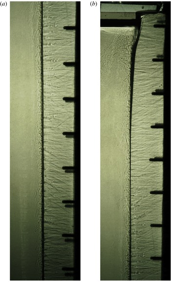
The wall plume visualised using the shadowgraph method with ice on the right and the salt water ambient on the left of each image. These photographs were presented in Kerr & McConnochie (Reference Kerr and McConnochie2015) and were taken from a qualitative experiment with a far-field temperature of $3.9\,^{\circ }\text{C}$ and salinity of 3.31 wt% NaCl. The vertical spacing of the black screws in the side walls is 6 cm. The photos show (a) the ice from a height of 32 cm up to 76 cm, and (b) the ice from a height of 72 cm to the free surface at 114 cm.

The experiments were conducted in a 1.2 m high, 1.5 m wide and 0.2 m long tank kept in a temperature-controlled room. Ice was grown from fresh water against one endwall and then exposed to salty water. The temperature and the salinity of the far field were varied to achieve different buoyancy fluxes, ${\it\Phi}$ , in different experiments. Buoyancy fluxes in the range ${\it\Phi}=(1.9{-}6.4)\times 10^{-7}~\text{m}^{2}~\text{s}^{-3}$ were achieved, giving Rayleigh numbers of $(3.6{-}8.9)\times 10^{13}$ .

Figure 1 shows photographs of an experiment with the flow visualised using the shadowgraph technique. The apparatus and experimental method are fully described in Kerr & McConnochie (Reference Kerr and McConnochie2015). Kerr & McConnochie (Reference Kerr and McConnochie2015) found that, when an ice wall dissolves into homogeneous salty water, the dissolution rate is uniform in the turbulent section of the flow. This behaviour corresponds to a uniformly distributed buoyancy flux and provides a convenient mechanism for testing (2.1)–(2.6).

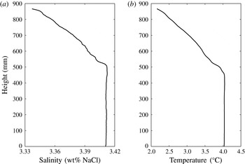
The position of the first front was measured using a conductivity–temperature probe that traversed vertically through the far field. Typical profiles of salinity and temperature are shown in figure 2. The first front measurement was based on the salinity profile, as it had a sharper first front due to the slower diffusion of salt compared to heat. Conductivity and temperature measurements were taken on the downward traverse to minimise the effect of mixing in the wake of the probe.

Figure 2.

Examples of a salinity and temperature profile made during an experiment. These particular profiles were made after 40 min and the experiment had a far-field temperature of $4.1\,^{\circ }\text{C}$ , a far-field salinity of 3.41 wt% NaCl and a buoyancy flux of ${\it\Phi}=4.0~\text{m}^{2}~\text{s}^{-3}$ .

Velocity measurements were made using a shadowgraph PTV technique. This technique is very similar to the schlieren particle image velocimetry (PIV) technique described by Jonassen, Settles & Tronosky (Reference Jonassen, Settles and Tronosky2006) with shadowgraph used instead of schlieren. It is also similar to the technique described in Crone, McDuff & Wilcock (Reference Crone, McDuff and Wilcock2008), although they used a significantly different method to compute velocity fields. All of these methods represent an adaptation of traditional PTV or PIV techniques in which turbulent eddies are tracked instead of traditional particles. The PTV software ‘Streams’ (Nokes Reference Nokes2014) was used for feature identification, particle matching and the computation of velocity fields.

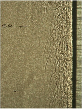
For shadowgraph PTV we used a zoomed-in camera window compared to figure 1. This provided higher resolution of turbulent features and enabled more accurate feature identification. An example of a shadowgraph PTV frame is shown in figure 3. The flow was filmed for approximately 10 s at each height and the resulting velocity fields were time-averaged. Averaging over longer periods of time was tested but did not change the results.

Figure 3.

A shadowgraph image of the wall plume as used for velocity measurement. The two black horizontal lines are 5 cm apart and the upper line is 50 cm above the base of the tank. The experiment had a far-field temperature of $4.3\,^{\circ }\text{C}$ and salinity of 1.94 wt% NaCl. The ice–water interface is at the left edge of the thick dark shadow and the ice is to the right.

The flow that we observed was very similar to the compressible turbulent boundary layer flow that Jonassen et al. (Reference Jonassen, Settles and Tronosky2006) investigated. Both flows have similar strengths and weaknesses regarding the use of shadowgraph PTV or schlieren PIV. Since both flows are primarily two-dimensional, the shadowgraph method provides an easily interpretable representation of the flow, which would not be true if there was significant flow variation through the light path.

Since the flow was highly turbulent, there were many eddies that could be tracked, giving the equivalent of an appropriate seeding density of particles in traditional PTV or PIV. However, near the edge of our rising plume, this ceased to be true. At the edge of the plume there were intermittent eddies, but these were not sufficient for shadowgraph PTV to be reliable. This was obviously also true in the quiescent far field. Finally, very near to the wall we were not able to properly resolve the eddies due to the refraction of light through the tank and the reflection of light off the ice. Within these limitations, we were able to obtain a reliable velocity profile around the location of maximum velocity. The velocity maximum was accurately measured and is the key feature of our investigation.

The buoyancy flux was defined as

(3.1) $$\begin{eqnarray}{\it\Phi}=V\frac{{\it\rho}_{s}}{{\it\rho}_{w}}\frac{g({\it\rho}_{f}-{\it\rho}_{w})}{{\it\rho}_{f}}(1-\mathscr{R}^{-1}),\end{eqnarray}$$

where $V$ is the measured dissolving velocity of the ice, ${\it\rho}_{s}$  is the density of the ice, ${\it\rho}_{w}$ is the density of fresh water at $0\,^{\circ }\text{C}$ , ${\it\rho}_{f}$ is the far-field density, $g$ is the acceleration due to gravity and $\mathscr{R}$ is the ratio of compositional to thermal buoyancy, defined as in Kerr & McConnochie (Reference Kerr and McConnochie2015) as

(3.2) $$\begin{eqnarray}\mathscr{R}=\frac{{\it\beta}S_{f}}{{\it\alpha}_{exp}[{\it\rho}_{w}L_{i}+{\it\rho}_{i}c_{i}(T_{iw}-T_{i})]/{\it\rho}_{f}c_{f}},\end{eqnarray}$$

where ${\it\alpha}_{exp}$ is the thermal expansion coefficient, ${\it\beta}$ is the equivalent coefficient for salt, $S_{f}$ and $c_{f}$ are the salinity and specific heat of the far field, $L_{i}$ , ${\it\rho}_{i}$ , $c_{i}$ and $T_{i}$ are the latent heat, density, heat capacity and temperature of the ice, and $T_{iw}$ is the temperature at the ice–water interface. The value of $T_{iw}$ was calculated using the turbulent dissolution model of Kerr & McConnochie (Reference Kerr and McConnochie2015).

The correction $(1-\mathscr{R}^{-1})$ is necessary since the compositional and thermal buoyancy act in opposing directions. By assuming that both buoyancy sources are well mixed inside the turbulent plume, the interaction is simplified.

It is possible that the combination of compositional and thermal buoyancy fields could lead to double-diffusive convection in this system. This has not been explicitly tested for but no evidence of double-diffusive convection was observed in these experiments. In the case of ice melting into a stratified ambient, double diffusion can result in horizontal intrusions (Huppert & Josberger Reference Huppert and Josberger1980; Huppert & Turner Reference Huppert and Turner1980) but this has not been observed in the case of a homogeneous ambient.

Measurements of the dissolving velocity, $V$ , have a standard deviation with height of 6 %. The far-field temperature and salinity, $T_{f}$ and $C_{f}$ , are known to the nearest $0.1\,^{\circ }$ C and 0.1 wt% NaCl, respectively. This uncertainty in far-field conditions translates to a maximum uncertainty in $({\it\rho}_{f}-{\it\rho}_{w})$ of 3 % and in $(1-\mathscr{R}^{-1})$ of approximately 6 %. All other constants in (3.1) have insignificant amounts of uncertainty. This translates to a 9 % uncertainty in the values of ${\it\Phi}$ .

4. First front measurements

We use the propagation of the first front with time to estimate a value of the entrainment coefficient, ${\it\alpha}_{P}$ , defined as in the model of Cooper & Hunt (Reference Cooper and Hunt2010). Equation (2.7) has been used to produce a quantity that depends linearly on time as shown in (4.1):

(4.1) $$\begin{eqnarray}3\left[\left(\frac{z_{0}}{H}\right)^{-1/3}-1\right]WH^{-1/3}{\it\Phi}^{-1/3}=C_{4}t.\end{eqnarray}$$

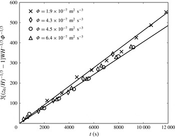
In figure 4 the left-hand side of (4.1) is plotted against time since the start of the experiment for four experiments with different buoyancy fluxes, ${\it\Phi}$ . Figure 4 is then used to estimate the volume flux constant, $C_{4}$ . The data in figure 4 have been shifted to force the curves through the origin. In the original data there were small offsets caused by a limited amount of dissolution before the experiment was started and by the conductivity profiles not being started at the exact start of the experiment. This offset was typically less than 300 s.

Figure 4.

The propagation of the first front throughout an experiment. The slope represents $C_{4}$ , with the two solid lines representing an entrainment coefficient of ${\it\alpha}_{P}=0.014$ and ${\it\alpha}_{P}=0.017$ or a volume flux coefficient of $C_{4}=0.040$ and $C_{4}=0.046$ .

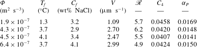
Table 1 gives the value of the volume flux constant, $C_{4}$ , as obtained from figure 4, along with the far-field conditions, the value of $\mathscr{R}$ and a computed entrainment coefficient, ${\it\alpha}_{P}$ , as defined in (2.5). As shown in figure 4 and table 1, we measure an entrainment coefficient of 0.014–0.017. This value is comparable with but smaller than that reported in Cooper & Hunt (Reference Cooper and Hunt2010) of 0.02–0.03. The observed entrainment coefficient will be redefined in § 6, using the velocity measurements described in § 5, such that the relationship $\text{d}Q/\text{d}z={\it\alpha}w$ is observed.

Our experiments are slightly different from those of Cooper & Hunt (Reference Cooper and Hunt2010), which could result in our reduced entrainment coefficient. The most significant difference is that, in their experiments, salty water was forced through a semipermeable membrane into still ambient fluid. This contrasts with our experiments, where the buoyancy diffused away from a very slowly retreating interface as the ice dissolved (measurements of the maximum plume velocity were typically around 5000 times larger than the dissolution velocity). The diffusive interface would have resulted in a gradual buoyancy profile across the laminar sublayer, while the advection at high Péclet number in the experiments of Cooper & Hunt (Reference Cooper and Hunt2010) would have resulted in a sharp change in buoyancy at the edge of the laminar sublayer.

We define a Péclet number as $V_{o}/({\it\kappa}_{c}/h_{c})$ , where $V_{o}$ is the advection velocity from the experiments of Cooper & Hunt (Reference Cooper and Hunt2010), ${\it\kappa}_{c}$ is the diffusion coefficient of salt and $h_{c}$ is the thickness of the diffusive compositional boundary layer as defined by Kerr & McConnochie (Reference Kerr and McConnochie2015). This Péclet number is the ratio between advective and diffusive transport through the diffusive compositional boundary layer. For our experiments $V_{o}=0$ so the Péclet number is also 0 and there is no advective transport through the compositional boundary layer. For the experiments of Cooper & Hunt (Reference Cooper and Hunt2010), however, the Péclet number is much larger than 1 (approximately 20 and 40 for their two buoyancy fluxes). Since this Péclet number is much larger than 1, the advection of salt will dominate the diffusion of salt through the laminar sublayer, and a sharp change in buoyancy is expected from the laminar sublayer to the turbulent plume. In contrast, our experiments should result in a gradually increasing salinity through the sublayer and into the plume.

Our apparatus could have resulted in more of the buoyant fluid being trapped near the wall than in the apparatus of Cooper & Hunt (Reference Cooper and Hunt2010). Trapping buoyant fluid near the wall could decrease the ability of the plume to entrain ambient water as the high-velocity fluid would also be trapped near the wall. We note that a diffusive interface will be present in both the case of room ventilation and the dissolution of Antarctic ice shelves and icebergs.

Table 1.

Volume flux coefficients, $C_{4}$ , entrainment coefficients, ${\it\alpha}_{P}$ , and ratio of compositional to thermal buoyancy, $\mathscr{R}$ , from first front data for four different buoyancy fluxes.

4.1. Stratification above the first front

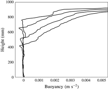
In addition to the position of the first front, the conductivity–temperature probe also regularly measured the stratification that formed above the first front. Figure 5 shows the stratification that develops with time during an experiment.

Figure 5.

Buoyancy profiles as measured by the conductivity–temperature traverser, showing the development of stratification above the first front with time. The profiles were taken 20, 40, 60 and 80 min after the start of the experiment, with the first front getting progressively lower over this time. Buoyancy is calculated as $g({\it\rho}_{e}-{\it\rho})/{\it\rho}_{e}$ , where ${\it\rho}_{e}$ is the ambient density below the first front and ${\it\rho}$ is the measured density.

The stratification that develops is approximately linear for most of the height above the first front. As the first front propagates down the tank, the stratification appears to weaken slightly. This approximately linear stratification with continuous buoyancy across the first front has been observed in many previous studies of turbulent plumes from distributed sources (Linden et al. Reference Linden, Lane-Serff and Smeed1990; Chen et al. Reference Chen, Li and Mahoney2001; Cooper & Hunt Reference Cooper and Hunt2010; Gladstone & Woods Reference Gladstone and Woods2014). Despite the strong experimental evidence that the buoyancy profile is continuous at the first front and approximately linear above it, many attempts at modelling these flows result in a step change in buoyancy at the first front and a nonlinear buoyancy profile above it (Linden et al. Reference Linden, Lane-Serff and Smeed1990; Cooper & Hunt Reference Cooper and Hunt2010). The discrepancy between experimental results and model predictions appears to be caused by a lack of detrainment in models. Without some mechanism for detrainment, a continuous buoyancy profile across the first front is not possible, which suggests that detrainment into the stratified interior is an important process in these plumes that must be included in any modelling efforts.

5. Velocity measurements

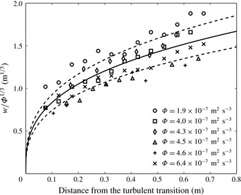
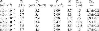
Figure 6 shows our measurements of maximum plume velocity plotted against distance from the turbulent transition, $z-Z_{turb}$ , where $Z_{turb}$ is the height where the plume becomes turbulent. The turbulent transition was typically between 10 and 15 cm from the base of the tank and the measured values are shown in table 2. The velocity measurements are scaled by ${\it\Phi}^{-1/3}$ so that the dependence on the buoyancy flux is clearly shown. Figure 6 shows that the velocity approximately follows the $w\sim {\it\Phi}^{1/3}$ scaling predicted by (2.3).

Figure 6.

Scaled maximum velocity measurements for all six experiments. The solid line shows $w=1.8{\it\Phi}^{1/3}z^{1/3}$ and the dashed lines show an uncertainty of one standard deviation. It is seen that the $w\sim {\it\Phi}^{1/3}$ scaling predicted by Wells & Worster (Reference Wells and Worster2008) and Cooper & Hunt (Reference Cooper and Hunt2010) describes the experimental results.

Table 2.

Maximum velocity constant, $C_{2,m}$ , from figure 7. Measured values are an average from all data points in figure 7. The uncertainty includes the entire range of measured values; $\mathscr{R}$ shows the ratio of compositional to thermal buoyancy in each experiment; and $Z_{turb}$ shows the distance between the base of the tank and the turbulent transition.

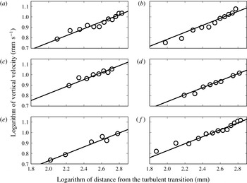
Figure 7 shows the logarithm of the data on figure 6 separated by experiment. On figure 7 the lines represent the $w\sim z^{1/3}$ scaling relationship predicted by (2.3) and (2.9). The data are consistent with this height scaling over the entire range of heights and buoyancy fluxes that were examined.

There was a small vertical volume flux through the turbulent transition so a virtual source that would be located at some point between the base of the tank and the turbulent transition should be used instead of $Z_{turb}$ . However, the strong agreement between the data plotted on figure 7 and the predicted $w\sim z^{1/3}$ scaling suggests that the virtual source is very close to the turbulent transition. There may be a small ${\it\Phi}$ dependence on figure 6. The experiments performed at lower values of ${\it\Phi}$ could involve a larger distance between the virtual source and $Z_{turb}$ , which would explain any ${\it\Phi}$ dependence on figure 6.

Figure 7.

Vertical velocities for experiments at six different ambient conditions. The solid lines show the predicted $w\sim z^{1/3}$ scaling from (2.3) and (2.9): (a) ${\it\phi}=1.9\times 10^{-7}~\text{m}^{2}~\text{s}^{-3}$ ; (b) ${\it\phi}=4.0\times 10^{-7}~\text{m}^{2}~\text{s}^{-3}$ ; (c) ${\it\phi}=4.3\times 10^{-7}~\text{m}^{2}~\text{s}^{-3}$ ; (d) ${\it\phi}=4.5\times 10^{-7}~\text{m}^{2}~\text{s}^{-3}$ ; (e) ${\it\phi}=4.6\times 10^{-7}~\text{m}^{2}~\text{s}^{-3}$ ; and (f) ${\it\phi}=6.4\times 10^{-7}~\text{m}^{2}~\text{s}^{-3}$ .

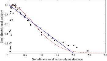
Table 2 shows derived values of the velocity constant, $C_{2,m}=w{\it\Phi}^{-1/3}z^{-1/3}$ , for each experiment. We measured an average value of $C_{2,m}$ across the six experiments of $1.8\pm 0.2$ . The velocity constant, $C_{2,m}$ , relates to maximum plume values and not to the top-hat values assumed in the model of Cooper & Hunt (Reference Cooper and Hunt2010). Based on the experimental observations of Cheesewright (Reference Cheesewright1968) and Vliet & Liu (Reference Vliet and Liu1969) shown in figure 8, a linear velocity profile is a very good approximation of the turbulent natural convection plume next to a uniformly distributed buoyancy source. With a linear velocity profile, a factor of $2/3$ is required to convert from a maximum velocity to a top-hat velocity such that both volume and momentum fluxes are conserved. The conversion from top-hat to physically realistic plume profiles is more fully explained in § 6. Our measurement of the top-hat value of $C_{2}$ is therefore $1.2\pm 0.1$ . The model of Cooper & Hunt (Reference Cooper and Hunt2010) predicts that $C_{2}\approx 3.7$ , based on our observations of the unadjusted entrainment coefficient, ${\it\alpha}_{P}=0.0155$ , which is approximately three times our observed value.

There are several explanations for this difference, some of which also explain the smaller measured entrainment coefficient discussed in § 4. Firstly, the diffusive interface could produce lower velocities. By trapping buoyancy closer to the wall, the velocity maximum may also be shifted closer to the wall. This is consistent with the natural convection boundary layer measurements shown in figure 8 (Cheesewright Reference Cheesewright1968; Vliet & Liu Reference Vliet and Liu1969), which show a velocity maximum that is very close to the wall. Such a velocity profile would result in a large drag force on the plume, which would result in decreased velocities.

In addition to this, the model of Cooper & Hunt (Reference Cooper and Hunt2010) assumes that viscous effects in the boundary layer adjacent to the wall are negligible. Regardless of the velocity profile, this will not be strictly true. Viscous effects from the wall must cause a no-slip boundary condition. Because of this, we would expect the top-hat velocity to be smaller than that predicted by (2.3).

6. Updated plume model

Using our measurements from §§ 4 and 5 we can construct a model for the turbulent wall plume that forms next to a vertically distributed source of buoyancy. The filling box measurements in § 4 give a volume flux, $Q$ , of

(6.1) $$\begin{eqnarray}Q=(0.043\pm 0.003){\it\Phi}^{1/3}z^{4/3},\end{eqnarray}$$

and the velocity measurements in § 5 give a maximum velocity, $w$ , of

(6.2) $$\begin{eqnarray}w=(1.8\pm 0.2){\it\Phi}^{1/3}z^{1/3}.\end{eqnarray}$$

Vliet & Liu (Reference Vliet and Liu1969) and Cheesewright (Reference Cheesewright1968) measured the vertical velocity profiles in the plume next to a constant-temperature plate. Their data are shown in figure 8 with both a linear and a Gaussian fit. Unfortunately, we are unable to plot our measured velocity data on figure 8, as the non-dimensionalisation used requires the full velocity profile, which we are unable to measure. In addition, we do not have access to the dimensional data measured by Vliet & Liu (Reference Vliet and Liu1969) or Cheesewright (Reference Cheesewright1968). As such, we are unable to compare our measured velocity profiles to those presented in figure 8. The velocity measurements in figure 8 show that the velocity profile is very close to linear, with a maximum velocity close to the wall and a very sharp shear layer between the wall and the point of maximum velocity.

Figure 8.

Vertical velocity measurements from Vliet & Liu (Reference Vliet and Liu1969) (hollow circles and triangles) and Cheesewright (Reference Cheesewright1968) (filled circles) from the rising plume next to a hot plate. Linear and Gaussian fits to the data are plotted in the blue solid line and red dashed line, respectively. The non-dimensional velocity is defined as $w/w_{max}$ and the non-dimensional distance is defined as $y/{\it\delta}^{\ast }$ , where ${\it\delta}^{\ast }=\int _{0}^{\infty }(w/w_{max})\,\text{d}y$ .

Based on their observations we have assumed that the velocity profile is linear, with the maximum velocity located at the wall. Appendix A copies the following analysis based on the assumption of a Gaussian velocity profile. Assuming a linear velocity profile, we can calculate the plume width, $b$ , and momentum flux, $M$ , as

(6.3) $$\begin{eqnarray}b=\frac{2Q}{w}=(0.048\pm 0.006)z\end{eqnarray}$$

and

(6.4) $$\begin{eqnarray}M=\frac{2Qw}{3}=(0.052\pm 0.007){\it\Phi}^{2/3}z^{5/3}.\end{eqnarray}$$

Equations (6.1)–(6.4) form a model of all plume properties, apart from the buoyancy, derived from our measurements of volume flux and maximum plume velocity. It is possible to construct an updated top-hat model from (6.1)–(6.4) that gives the following equations for the top-hat velocity, $w_{T}$ , width, $b_{T}$ , and buoyancy, ${\it\Delta}_{T}$ :

(6.5) $$\begin{eqnarray}\displaystyle & \displaystyle w_{T}=\frac{2w}{3}=(1.2\pm 0.1){\it\Phi}^{1/3}z^{1/3}, & \displaystyle\end{eqnarray}$$

(6.6) $$\begin{eqnarray}\displaystyle & \displaystyle b_{T}=\frac{Q}{w_{T}}=(0.036\pm 0.005)z, & \displaystyle\end{eqnarray}$$

(6.7) $$\begin{eqnarray}\displaystyle & \displaystyle {\it\Delta}_{T}=\frac{F}{Q}=(23\pm 2){\it\Phi}^{2/3}z^{-1/3}. & \displaystyle\end{eqnarray}$$

We now recalculate the top-hat entrainment coefficient, ${\it\alpha}_{T}$ , such that the equation

(6.8) $$\begin{eqnarray}\frac{\text{d}Q}{\text{d}z}={\it\alpha}_{T}w_{T}\end{eqnarray}$$

is consistent with our measured velocity. An updated value of ${\it\alpha}_{T}$ is necessary, as we are not directly measuring an entrainment coefficient in § 4 but are instead measuring $Q(z)$ , which also depends on the plume velocity. The original calculation of ${\it\alpha}_{P}$ was made using the plume volume flux given in (2.3). Using our measured value of $w_{T}$ results in the following expression for ${\it\alpha}_{T}$ :

(6.9) $$\begin{eqnarray}{\it\alpha}_{T}=\frac{1}{w_{T}}\frac{\text{d}Q}{\text{d}z}=0.048\pm 0.006.\end{eqnarray}$$

One of the implications of our updated plume model compared with the model of Cooper & Hunt (Reference Cooper and Hunt2010) is that there must be a significant drag force acting on the plume. This drag is represented as ${\it\epsilon}$ in equation (2.1) of Cooper & Hunt (Reference Cooper and Hunt2010) and it is assumed to be negligible when formulating the solution given in our (2.1)–(2.6). By assuming negligible drag, the upwards buoyancy force was balanced by the gain in momentum flux in the plume, which led to the much larger velocity predictions than were observed in our experiments. We calculate the value of this drag as

(6.10) $$\begin{eqnarray}{\it\epsilon}=b_{T}{\it\Delta}_{T}-\frac{\text{d}M}{\text{d}z}=(0.75\pm 0.12){\it\Phi}^{2/3}z^{2/3},\end{eqnarray}$$

which represents approximately 90 % of the upward buoyancy force. Based on the velocity profiles of Vliet & Liu (Reference Vliet and Liu1969), such a high value does not seem unreasonable, as the velocity profile shows a maximum velocity very near to the wall, with a sharp shear zone between the wall and the velocity maximum. Such a profile would induce significant drag on the plume and result in a very high wall shear stress. Turbulent fluctuations within the plume would also cause a large amount of turbulent drag within the plume.

7. Physical application

We now use (6.1)–(6.3) to calculate maximum plume widths, velocities and Reynolds numbers for a typical dissolving iceberg and a typical room.

In the case of an Antarctic iceberg, we take a typical ocean temperature of 1  $^{\circ }$ C (Budd, Jacka & Morgan Reference Budd, Jacka and Morgan1980). Following the equations of Kerr & McConnochie (Reference Kerr and McConnochie2015) for ablation velocity and interface conditions, this gives a buoyancy flux, ${\it\Phi}$ , of $1.7\times 10^{-7}~\text{m}^{2}~\text{s}^{-3}$ . Tabular icebergs in the polar oceans frequently sit several hundreds of metres deep in the water column. At a characteristic iceberg height of 200 m (Dowdeswell & Bamber Reference Dowdeswell and Bamber2007), the turbulent plume next to such an iceberg would have a width, $b$ , of $9.6\pm 1.2$  m, a maximum velocity, $w$ , of $0.058\pm 0.006$  m s $^{-1}$ , and a Reynolds number, defined as $\mathit{Re}=Q/{\it\nu}$ , where ${\it\nu}$ is the kinematic viscosity, of $(2.8\pm 0.2)\times 10^{5}$ . These calculations should guide any attempts to observe this rising meltwater plume in the field. In particular, it would be useful to have velocity, temperature and salinity measurements from within the plume next to an iceberg or ice front.

In the case of a room with a heat flux through a wall or window, we calculate a Rayleigh number, $\mathit{Ra}$ , of $3.2\times 10^{10}$ based on a temperature difference of 10  $^{\circ }$ C between the interior and the exterior, an ambient temperature of 20  $^{\circ }$ C and a height of 3 m. For simplicity we have assumed that the buoyancy source comprises the entire height of the room to maintain a similar configuration to our experiments. For turbulent natural convection on an isothermal vertical boundary layer, the Nusselt number, $\mathit{Nu}$ , is given by $\mathit{Nu}=0.10\mathit{Ra}^{1/3}$ (Holman Reference Holman2010, p. 355), which gives a Nusselt number of 317. We can use the Nusselt number to calculate a buoyancy flux as ${\it\Phi}=(\mathit{Nu}{\it\kappa}{\rm\Delta}Tg)/(HT)$ , where ${\it\kappa}$ is the thermal diffusivity, ${\rm\Delta}T$ is the applied temperature difference, $g$ is gravity, $H$ is the height of the room and $T$ is the ambient temperature in kelvin. This gives a buoyancy flux, ${\it\Phi}$ , of $6.7\times 10^{-4}~\text{m}^{2}~\text{s}^{-3}$ . Using this value and the maximum height of 3 m, we obtain a plume width, $b$ , of $0.14\pm 0.02$  m, a maximum plume velocity, $w$ , of $0.23\pm 0.03$  m s $^{-1}$ , and a Reynolds number of $(1.1\pm 0.1)\times 10^{3}$ .