CALCULATION OF NATIONAL STATISTIC

Initially, the Civil War and Reconstruction income tax did not cover the states that made up the Confederacy. However, as these states were pulled back into the Union's fold, they became subject to the tax. For the years after the Civil War when the tax was still in operation, we can calculate the percent of total income accruing to the top 1 and 0.1 percent of tax units, which are defined as an adult male, 22 years of age or older, and all of his dependents. The formula is as follows:

(1)

Due to data problems, a number of assumptions are required to calculate the statistic. We can calculate the number of tax units that made up the top 1 and 0.1 percent by estimating the adult male population. There are census figures in 1860 and 1870, and we can form estimates for the intervening years using a linear trend.Footnote ² On the one hand, due to war-related deaths and decreases in immigration, a linear trend likely overestimates the adult male population in the middle of the decade. This creates an upward bias in the estimated number of tax units in the top 1 and 0.1 percent and in the estimated income share statistics. On the other hand, because of the tumultuous nature of Reconstruction, the 1870 population statistic could be lower than the actual population. That would bias the income share statistics downward.Footnote ³

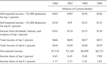
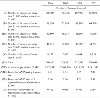
We also need to calculate the total income accruing to the top 1 and 0.1 percent. Collection of income tax depended on the source of income and types of employment. For civil, military, and naval personnel and all income derived from interest, coupons, and dividends from all banks, trust companies, savings institutions, insurance companies, and railroads, taxes were collected at the source.Footnote ⁴ For all other incomes, individuals self-reported and paid taxes. The Commissioner of Internal Revenue published the total amount of revenue by year, which can be used to generate total self-reported income of all the US adult male taxpayers—about 3 percent of the adult male population. For the 1866 to 1869 period, the Commissioner also compiled figures that allow us to delineate the 97^th, 98^th, 99^th, and 99.9^th percentiles.Footnote ⁵ Estimates for the total self-reported income of the top 1 and 0.1 percent of adult males and their dependents are displayed in the first and second rows in Table 1.

Table 1

CONSTRUCTION OF INCOME SHARE OF TOP 1 PERCENT AND TOP 0.1 PERCENT OF TAX UNITS

Source:

See text.

The Commissioner reported aggregate data on taxes collected from income from dividends, interest, and coupons by fiscal year.Footnote ⁶ Because of the non-synchronization of collection after the act of 1867, the total amount collected during a given fiscal year covers parts of two calendar years. But as one can see from the calculations in Table 1, assuming that a given fiscal year represents the corresponding calendar years leads to similar income share statistics for the three years.

Unlike self-reported statistics, there is no way to identify what part of income deriving from dividends, interest, and coupons accrued to the top 1 and 0.1 percent. However, we can make rough estimates and give ranges for sensitivity. Because of the relatively low concentration of wealth in 1870 and the differences in portfolio holdings and earnings for upper income groups, it is likely that somewhere between 55 and 65 percent of income from dividends, interest, and coupons accrued to the top 1 percent of tax units.Footnote ⁷ Using the middle of this range, I calculate the total amount of such income flowing to the top 1 percent. The result is displayed in the third row in Table 1. We can form upper bound estimates of the percent of income from dividends, interest, and coupons that accrued to the top 0.1 percent by assuming they received all of the income that flowed to the top 1 percent.

The sum of the total amount of self-reported income and income collected at the source accruing to the top 1 and 0.1 percent are displayed in the fourth and fifth rows in Table 1. To calculate the income shares, we need the nominal gross domestic product (GDP). Robert Gallman (Reference Soltow1966) calculated nominal GDP figures for 1859 and 1869, and Louis Johnston and Samuel Williamson (Reference Johnston and Williamson2013) interpolated values for the intervening years. To convert GDP to total national income, we need to deduct capital depreciation and non-taxable incomes, which account for somewhere between 10 and 20 percent of GDP.Footnote ⁸ The results are shown in the sixth row in Table 1.

The income shares of the top 1 and 0.1 percent of tax units are displayed in the last two rows in Table 1. The top 1 percent received 8.63 and 8.45 percent of all income in 1866 and 1867, respectively. The income share of the top 1 percent increased to 9.4 percent in 1868 and 9.98 percent in 1869. If we assume a much larger percent of income from dividends, interest, and coupons accrued to the top 1 percent, say 80 percent, their share of total income would change to 9.1 percent in 1866, 9.0 percent in 1867, 9.9 percent in 1868, and 10.6 percent in 1869. The statistic for the top 0.1 percent followed a similar trajectory starting at 3.17 percent in 1866, falling in 1867, and increasing to 3.85 percent by 1869. If we assume that 80 percent of the income from dividends, interest, and coupons accrued to the top 0.1 percent, their share of total income would change to 3.60 percent in 1866, 2.88 percent in 1867, 3.98 percent in 1868, and 4.47 percent in 1869.

COMPARABILITY OF STATISTICS

Four points need to be clarified. First, salaries of federal government employees were taxed at the source and are not included. This exclusion does not seem to be a significant problem, as the federal government was much smaller during this period and it is unlikely that federal salaries made up a significant portion of income of the top 1 and 0.1 percent. Second, only capital gains from assets held less than three years are included in self-assessments. Thus this series is awkwardly in the middle of Thomas Piketty and Emmanuel Saez's series (Reference Piketty and Goldhammer2003), which neatly include and exclude capital gains. Third, individuals who owned their houses were allowed to estimate what rent would be and deduct it from their income, which biases the statistics downward.

Fourth, to the degree that the top 1 and 0.1 percent of the population under reported their incomes, the total income of these groups would be less and thus our calculations for the percent of total income accruing to these groups would be downwardly biased. Undoubtedly, this is the case to some degree. However, what is important here is the relative level of tax fraud in 1866, 1867, 1868, and 1869, compared to present-day tax fraud. I will focus on refuting arguments that income tax fraud was exceptionally large from 1866 to 1869.

Some contemporaries identified fraud and evasion as a significant and growing problem. Such arguments were especially popular with politicians who opposed the income tax and saw it as a cause of dishonesty and corruption (Hill Reference Hill1894). “Complaints continue to be received at this office that many persons liable to income tax fail to make full returns,” explained Joseph Lewis, commissioner of the Bureau of Internal Revenue, in early 1865.Footnote ⁹ “American ingenuity was never more strikingly illustrated - not even by the exhibits of the patent office,” insisted David Wells, who Congress appointed to investigate the federal tax system, “than it was [from 1867 to 1872]… in devising and successfully carrying out methods for evading the taxes on income and distilled spirits” (Wells Reference Wells1874). For the second half of the 1860s, this conclusion was based on a falling nominal value of self-reported income.

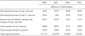
Total self-reported income did decrease almost every year after 1864, except in 1868 and 1869. Some of this decrease was a result of an increase in the minimum amount exempted. From 1862 to 1865, $600 was exempted from taxation, whereas from 1866 to 1869, the amount exempted was $1,000. In addition, there was deflation averaging 6.5 percent per year between 1866 and 1868 (Johnston and Williamson Reference Johnston and Williamson2013). Thus nominal self-reported income would be expected to decrease unless we assume income inequality was increasing. In Table 2, I display the real value of self-reported income of the top 1 and 0.1 percent of tax units in 1866 dollars.

Table 2

REAL INCOME OF TOP 1 PERCENT AND TOP 0.1 PERCENT

Source:

See text.

In addition, income deriving from dividends, interest, and coupons increased in both nominal and real terms (see Tables 1 and 2). Thus, if we take these two factors together and look at the total real income of the top 1 and 0.1 percent of tax units, we see that although incomes for these groups decreased in 1867, they increased more dramatically in 1868 and 1869.Footnote ¹⁰

Other contemporaries thought that tax fraud was minimal. “[T]he most signal pecuniary success has attended the operations of the bureau” to stamp out income tax fraud, explained the New York Times (2 June 1865, p. 1). The American News Company, which published a the list of New Yorkers' reported taxable income in 1863, wrote “In England, it is estimated by an able writer on taxation that the government is defrauded of full one third of the taxes due … We do think that in this county it will amount to no more than one tenth, and much of that results from ignorance rather than a desire to defraud.”

Over the decade, the Bureau of Internal Revenue received increased powers to fight fraud. The Revenue Act of 1865 empowered the assistant assessor to increase any individual's self-reported income, even if the individual had taken an oath as to the verity of the amount reported. The Act also created fines for non-compliance. For failure to file a return, taxpayers were charged a penalty of 25 percent of taxes due. The Revenue Act of 1867 increased the penalty to 50 percent of taxes due; for false returns, taxpayers were charged 100 percent of taxes due (Ratner Reference Ratner1942). To detect fraudulent returns, revenue officials were given “the right to enter premises, take books, examine accounts, shut up shops, swear witnesses, and send for persons and papers and exact fines through the medium of the courts” (New York Times, 2 June 1865, p. 1).

While some contemporaries identify the Civil War income tax with substantial fraud, it does not seem that tax fraud was exceptional in 1866, 1867, 1868, and 1869. The decrease in the nominal value of self-reported income was at least partially a result of the fall in the price level, and income collected at the source increased substantially both in real and nominal terms.

COMPARISON WITH CURRENT DATA

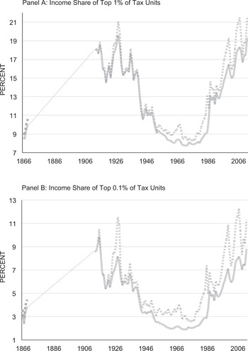
In Figure 1, I display Piketty and Saez's data (Reference Piketty and Saez2003) for the income share of the top 1 and 0.1 percent between 1913 and 2012 with the statistics calculated here. The double solid line represents Piketty and Saez's series that excludes capital gains and the checked line includes capital gains. The light double lines in the left edge of the graphs are the statistics for the income share of the top 1 and 0.1 percent of tax units from 1866 through 1869; the hard dash line are the upper bound estimates. As we can see, the income shares of the top 1 and 0.1 percent of tax units during the late 1860s were significantly lower than during the 1910s. Indeed, they represent lows in US history comparable to the late 1960s and early 1970s. Even assuming a much larger percent of income from dividends, coupons, and interest accrued to the top 1 and 0.1 percent, the findings do not change fundamentally.

Figure 1

INCOME SHARE OF TOP 1 PERCENT AND TOP 0.1 PERCENT

Source: See text.

These results are contrary to Soltow (Reference Soltow1969). However, they fit with both our contemporary understanding of inequality and economic turmoil and our impressionistic view of inequality during the Gilded Age—the decades spanning from Reconstruction to the end of the nineteenth century. In terms of the first point, the low levels of inequality could be the result of short-term fluctuation stemming from economic turmoil resulting from the Civil War and Reconstruction. Several studies on income inequality in the twentieth and twenty first centuries have shown that economic turmoil and business downturns cause high incomes to fall disproportionately and thus reduce income inequality, at least in the years immediately after a crisis (Piketty and Saez Reference Piketty and Saez2003; Goldin and Margo Reference Goldin and Margo1992). The years after 1865 were plagued by recession and deflation. Real GDP fell by 4.6 percent between 1865 and 1866. Not until 1868 did real GDP surpass its 1865 peak. Between 1864 and 1868, the price level fell 18.2 percent. If we look through the lens of current studies, we would expect these developments to lead to low levels of income inequality. At the same time, it is not clear that wealth holdings were the same during the 1860s as during the twentieth and twenty-first century. A different wealth structure could mean that capital income responded differently to economic downturn and thus a potentially different relationship between recession and inequality.

It could also be that these low levels of inequality were a result of the immense institutional change of the 1860s. The Civil War led to the destruction of slavery. Its effects can be seen through an examination of wealth statistics. In 1860, southern men made up 59 percent of the wealthiest 1 percent of adult males in the United States; ten years later, their share had fallen to 18 percent. Average real wealth of white southern males decreased from $3,978 in 1860 to $1,440 in 1870 (Soltow Reference Soltow1976, pp. 65 and 101). The planter class was decimated by the destruction wrought on Southern land and animals and the liberation of its most prized asset, slaves. To the degree that bondage was destroyed and African Americans experienced an increase in economic freedom, income inequality would have changed. Indeed, in 1866, Congress abrogated the nascent Presidential Reconstruction system, which allowed white southerners significant freedom in re-subjugating the newly freed slaves. In its place, Congress empowered African Americans through the Freedman's Bureau and other institutions leading to unheard of economic freedom. Laws were put in place to shift risk from fluctuation in crop yields to creditors and landlords, to allow farmers to sell crops to the highest bidder, and much more (Foner Reference Foner1988).

Furthermore, during the 1860s, the federal government was taxing the rich more than ever before. In 1862, for the first time in the history of the United States, individuals had to pay a federal tax on income earned. Dividends, interest, and coupons were taxed. In the same year, the federal government passed a tax on inheritance. Even business gross revenue was taxed. Indeed, there is ample evidence that these laws were adopted with the intent to equitably distribute the tax burden.Footnote ¹¹

If the low levels of income inequality in the late 1860s were a result of institutions change, then inequality would have increased more slowly throughout the final decades of the nineteenth century. This understanding is in line with our impressions of increasing inequality during the Gilded Age and works like Stelzner (Reference Stelzner2015), Forbath (Reference Forbath1991), Woodword (Reference Woodward1951, 2001), Blackmon (Reference Blackmon2008), and a number of other authors that argue that institutions became increasingly more regressive during the late nineteenth century.

In this article, I cannot say with certainty what created these low levels of inequality during the late 1860s. Future studies will have to enlighten this debate. However, whether short-run economic turmoil or long-run institutional change, it make sense that the income share of the top 1 and 0.1 percent of tax units reached such low numbers in 1866, 1867, 1868, and 1869.