Early Japanese Industrialization and Exports, 1880–1910

The Japanese economy began to industrialize in the second half of the nineteenth century, following its forced opening to international trade in the 1850s by western powers. Despite a modest natural resource endowment, an economy based on subsistence agriculture, and a political revolution culminating in the 1868 Meiji Restoration, over the next half century the economy rapidly increased its manufacturing share and trade volumes to become the region’s leader in modern economic growth and ultimately the first non-western, industrial economy. By around 1900, Japanese manufacturing as a share of total output matched that of the United States, with an increasing emphasis on more capital and resource intensive sectors (Perkins and Tang Reference Perkins and Tang2017). This was owed in part to substantial investment in domestic infrastructure like railroads, which increased scale and agglomeration economies (Tang Reference Tang2014), and the country’s adoption and diffusion of foreign technologies, which matched or exceeded that of leading industrial economies like the United States (Nicholas Reference Nicholas2011; Saxonhouse Reference Saxonhouse1974; Tang Reference Tang2016).

Modernization of the domestic economy occurred alongside dramatic growth in trade, with Japan starting from virtual autarky in the mid-nineteenth century and averaging nominal growth of more than 9 percent per annum in the four decades up to WWI (Japan Statistical Association 1987). Exports and imports rose in tandem and were mostly balanced over the period, with trade accounting for a quarter of value added output by the early 1900s. The composition of that trade, however, changed significantly and in part reflected the evolving structure of domestic production. Foremost among the modernizing industries was textiles, which was consistently the largest export earner and adopter of foreign technologies (Makimura Reference Makimura2017; Saxonhouse Reference Saxonhouse1974). Exports within this broad sector shifted from raw materials (e.g., silk cocoons) to higher valued-added products like finished fabrics and apparel while the opposite occurred in imports (Perkins and Tang Reference Perkins and Tang2017). The importance of higher value-added textiles is highlighted by cotton thread, which in 1910 was the single largest export and represented 42 percent of all exports, with silk fabrics and textiles taking second place with 8.5 percent of exports. Trade in minerals, processed metals, and machinery exhibited a similar but less marked transition, with exports of higher valued-added goods increasing and imports of the same decreasing in share over time.

Upgrading in value-added production might be considered surprising given Japan’s lack of tariff autonomy until the first decade of the twentieth century, which owed to a series of “unequal” treaties signed with the leading European countries and the United States. Until the end of the nineteenth century, Japanese tariff protection averaged below 4 percent, gradually doubling over the first decade of the twentieth century until the war. Given the country’s inability to protect its nascent modern manufacturing sectors during its period of rapid industrialization and trade expansion, Japanese trade policy is unlikely to have affected observed trade patterns.

Ricardian comparative advantage or a factor endowment driven theory of trade are also seemingly insufficient to explain Japan’s emerging prowess in manufacturing as they would predict Japan specializing in raw silk and low-skill labor-intensive manufactures (Williamson Reference Williamson2011; Galor and Mountford Reference Galor and Mountford2008).Footnote ² Instead, trade costs may more plausibly explain Japan’s reorientation away from European markets. Asia was much closer and the United States had just completed its transcontinental railroad in 1869, opening up direct trade routes to Asia from its West coast. Over this period, there were also a number of exogenous events that facilitated Japanese exports such as pebrine disease, which wiped out European raw silk production in the mid-nineteenth century, and unexpected victories in the 1894–1895 Sino-Japanese and 1904–1905 Russo-Japanese wars. The wars provided Japan with its first imperial colony of Taiwan and privileged access to Chinese resources and markets.Footnote ³ Formal annexation of Korea in 1910 only furthered Japan’s political and commercial ambitions.

Most analysis of Japanese trade has focused on national aggregates or limited numbers of products, which are useful in understanding general trade patterns and potential welfare gains from trade, but neglect the detail available in more disaggregated trade statistics. In particular, aggregated series are unable to explain the timing of entry into particular markets, the sequencing of market entry, and the particular goods exported to a particular country. For example, greater variation within a product category (e.g., quality, unit price) may provide evidence about the types of goods demanded by different markets, so even if low cost Japanese labor mitigated productivity or trade cost disadvantages as a whole, it is unclear that the composition of exports would be similar across trade partners. Moreover, consumers in wealthier countries prefer relatively expensive high quality manufactures compared to poorer economies (Hallak Reference Hallak2006), which may explain why exports of comparatively cheap, low-quality Japanese manufactures expanded faster in low income markets.Footnote ⁴

In sum, to become internationally competitive, Japan not only had to invest in domestic infrastructure and navigate international economic and political changes, but also reduce trade costs and produce differentiated products for its various trade partners. In the absence of equivalently detailed domestic output data, we use highly detailed export data as their proxy to show how the economy changed over time and to identify which factors were more likely to have contributed to the observed patterns of export growth.

Data: Disaggregated Exports for Japan, 1880–1910

Our article is the first to digitize and analyze the universe of bilateral, product-level data for Japanese exports every five years from 1880 until 1910 (Meissner and Tang, Reference Meissner and Tang2018). The data sources are the official trade returns from Japan’s customs bureau, which collected the data annually starting in the 1870s (Ministry of Finance 1880–1910). Until the 1880s, data collection was inconsistent and incomplete, but thereafter data quality improved significantly. The data provide export destination, total value, quantity, and physical unit measures for some products, and a text-based product description. To classify these data, we hand-coded each product with a unique SITC Revision 2 classification. While some products can be described up to the five-digit level, the majority of the products are classified at the three-digit level of disaggregation. We use this level in our analysis as it captures more than 95 percent in value for each year of data and thus is representative of the cross section of exports over the entire period.Footnote ⁵ Furthermore, using the standardized three-digit classification level allows us to compare products across all types of exports consistently and to estimate results using standard statistical methodologies. The Online Data Appendix lists the 440 products by their original description and the associated SITC three-digit classification. Since the Japanese classification is significantly finer than the SITC three-digit categorization, there may be some under-estimation of the trends in growth of new products.

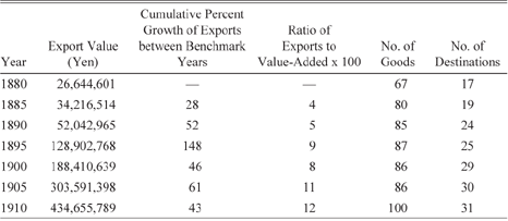
Even so, in our starting year of 1880, Japan exported 67 unique goods at the three-digit level and by 1910 this increased to 100. Over the same period, there were a total of 116 goods exported since some appeared and later disappeared; only 100 remained active in 1910. We retain exiting goods in our data because in principle such goods could be re-launched and “zeroes” provide information about the inability to sell in export markets. In terms of destinations, we have up to 76 potential destinations. The 76 destinations are those from Michael Huberman, Christopher M. Meissner, and Kim Oosterlinck (Reference Huberman, Meissner and Oosterlinck2017). Japan actively exported at least one product to 17 different countries in 1880. In 1910 the number stood at 31. There were no partner exits. Forty-five of the 76 destinations never imported from Japan in this period according to official Japanese sources. We classify them as receiving no exports from Japan. For these 45 destinations, we collect as much information as possible on trade costs and market size, which we describe later, since these effective “zeroes” also provide information about when trade costs were prohibitively high.

Table 1 provides the nominal value of trade, ratio of exports to value-added, number of active destinations, number of active product lines, and number of distinct goods that could be potentially exported. Although the scaling by value-added gives a sense of real trade growth, we generally do not deflate the nominal trade data since many of our comparisons will be within product comparisons and time dummies in our regression models sweep away variation coming from common price trends. Export price indices are available in principle or can be constructed from our data, but since the focus of our article is on new goods, designing an appropriate export price index to properly account for new goods with these data would be a challenge. In addition, goods without uniform physical quantities are difficult to include in such price indices and these include significant goods in the manufactured goods list. In contrast to Simon Evenett and Anthony Venables (Reference Evenett and Venables2002) who restrict attention to trade values above several thresholds given data errors and one-off exports, we use all available data for our study.

Table 1

Summary of Japanese Exports, 1880–1910

Note: Goods are measured at the three-digit SITC (Rev. 2) level. Value is in nominal yen. Columns for goods and destinations are for active exports and are a subset of the universe of goods that were ever exports over the period (e.g., by 1910 there were 116 distinct goods that had been exported).

Source: Ministry of Finance (various years) and authors’ calculations. Value added data, which begins in 1885, are from Ohkawa, Takamatsu, and Yamamoto (Reference Ohkawa, Takamatsu and Yamamoto1974).

Besides the disaggregated trade data, we have also assembled a database with variables that proxy for trade costs used in the empirical trade literature. The first is maritime shipping distances in nautical miles. We have information for three leading ports in Japan: Nagasaki, Yokohama, and Kobe. Distances are also available for multiple ports for some destination countries (e.g., China). We use the simple average shipping distance across all Japan-partner pairs in our data (Whittingham and King Reference Whittingham and King1947).Footnote ⁶ We also hand-collected Japanese diplomatic representation abroad and foreign diplomatic representation in Japan from the Almanach de Gotha (Reference Almanach de Gothavarious years). We record the presence of consular or diplomatic staff in each country or in Japan by using the yearbook’s detailed biographical list of such staff.

Finally, we include information on whether Japan had a fixed exchange rate with a destination because exchange rate uncertainty and volatility have been cited as important to trade costs in the literature (Estevadeordal, Frantz, and Taylor Reference Estevadeordal, Frantz and Taylor2003; López-Córdova and Meissner Reference López-Córdova and Meissner2003; Mitchener and Weidenmier Reference Mitchener and Weidenmier2008; Mitchener and Voth Reference Mitchener and Voth2011). These data are from Christopher M. Meissner (Reference Meissner2003) and Lawrence H. Officer (Reference Officer2014), while data on whether a destination had signed a treaty with a Most-Favored Nation (MFN) clause with Japan are from the House of Commons (1908), Ministry of Foreign Affairs, Japan (1918), and the United States Tariff Commission (1922). In terms of market characteristics, we use real GDP and population from the Angus Maddison project (Reference Maddison2015). We also supplement some population data not in Maddison from the Almanac de Gotha yearbooks.

Decomposition: Diversification of Japanese Exports

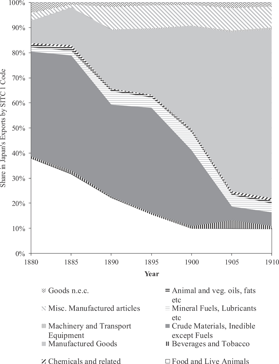
Between 1880 and 1910, Japan diversified its exports on two major dimensions: from mainly exporting raw and low value added commodities to manufactured goods, and from serving its near neighbor China and leading rich countries in Europe and the United States to a broader set that included smaller and poorer Asian economies. As shown in Figure 1, Japanese exports in primary products (e.g., food and live animals, non-food crude materials, fuel) steadily fell from more than 80 percent in 1880 to less than 20 percent by 1910. General manufactured goods (e.g., textiles, furniture, and household items) rose from less than 10 percent of exports to nearly 70 percent in 1910, with the remainder comprising machinery and miscellaneous manufactures. Initially, Japan focused on exporting non-fuel raw material, principally raw silk and silk waste as well as food and animal products. Manufactures including cotton thread, other cotton products, and finished silk goods amongst other manufactured goods dominated Japanese exports by 1910.

Figure 1

Share of Exports by SITC One-Digit Category

Notes: Figure shows the total export share in each one-digit SITC (Rev. 2) category. Note that the order of the products from top-to-bottom within the figure corresponds to the ordering on the legend from top-to-bottom. Source: Ministry of Finance (various years) and authors’ calculations.

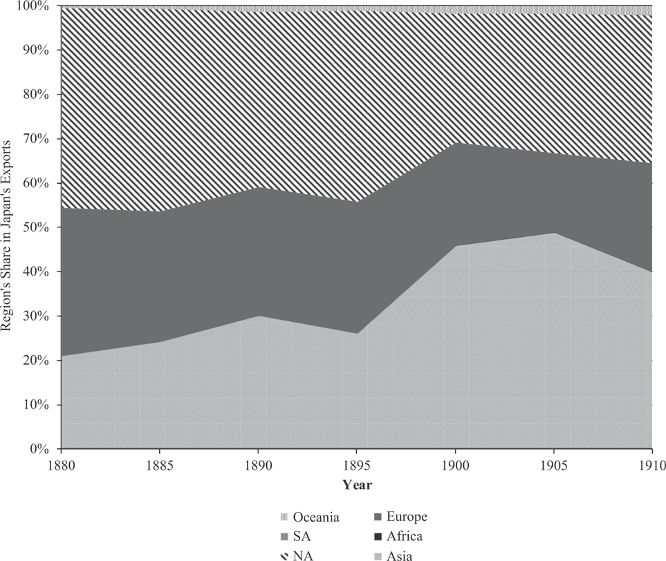
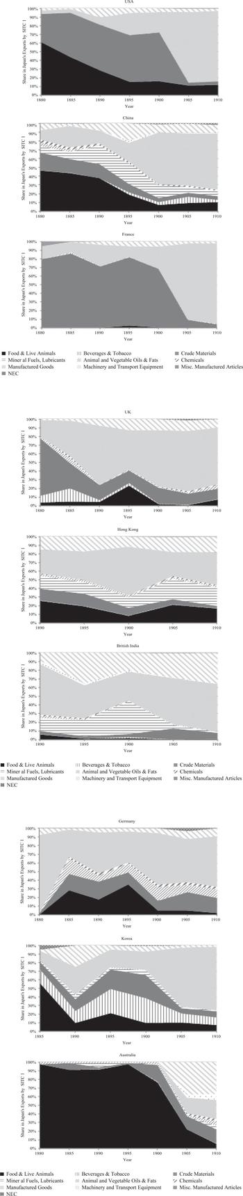
With regard to export destinations, Figure 2 shows falling shares of total exports for North America (i.e., United States) and Europe, from nearly 80 percent of total exports in 1880 to 60 percent by 1910. Asian countries extend their export share from 20 percent in 1880 to nearly 40 percent by 1910, with Chinese dominance within Asia fading.Footnote ⁷ Trade with Oceania (i.e., Australia) was small but rising. This is consistent with a Herfindahl index of concentration, which decreases from 0.3 to 0.2 between 1880 and 1910.Footnote ⁸ Combining both dimensions of commodity type and export destination for Japan’s top export markets, all exhibit the same pattern of increased manufacturing share as shown in Figure 3.

Figure 2

Share of Six Regions in Japan’s Exports, 1880–1910

Notes: Figure shows the total export share for six regions for Japanese exports. Source: Ministry of Finance (various years) and authors’ calculations.

Figure 3

Share of Exports by SITC One-Digit Category for Top Nine Destinations

Notes: Figures plot the share of total exports by value for all ten SITC one-digit codes on the y-axis. The x-axis covers every five years between 1880 and 1910. Source: Ministry of Finance (various years) and authors’ calculations.

These two extensive margins of export growth have been investigated in recent theoretical and empirical trade research as ways to explain changes in trade flows (Chaney Reference Chaney2008; Eaton and Kortum Reference Eaton and Kortum2002; Helpman, Melitz, and Rubinstien Reference Helpman, Melitz and Rubinstein2008; Huberman, Meissner, and Oosterlinck Reference Huberman, Meissner and Oosterlinck2017; Melitz Reference Melitz2003). The rationale for doing so is that in nearly all models of trade, (e.g., Ricardian, factor endowment, and those driven by a love of variety) trade costs matter for the direction of trade.Footnote ⁹ Not only do trade costs determine the amount of each product shipped, but they also determine whether a product or destination is “active” since fixed entry costs must be covered for firms to be willing to ship to a destination.

Furthermore, intra-industry trade is well-documented and nations at similar stages of development engage in significant trade even during the first age of globalization. Often factor-endowment driven models as well as Ricardian models assume that countries source a good from the single cheapest supplier, implying “complete specialization,” which was true neither in the nineteenth century nor today. Given multiple suppliers of a particular product in a destination market (e.g., Chinese and Japanese silk in the United Kingdom), it may be the case that quality matters such that even ostensibly high price producers (low productivity or high quality) can compete with sellers offering lower prices associated with either high productivity or low quality.

The underlying theory provides direction to explore which determinants were responsible for Japanese export growth. In particular, following Jonathan Eaton et al. (Reference Eaton, Eslava and Kugler2008), one can decompose exports by their extensive and intensive margins, the former being expansion in new products or trade partners and the latter in existing trade relationships. Formally, we decompose the percentage growth of exports (X) into goods by trade partner that continue from previous years, those that enter, and those that exit. Formally we have:

${{{X_{dt}} - {X_{dt - 1}}} \over {{X_{dt - 1}}}} = \left( {{{{\Sigma _{k \in CN_d^{t - 1,t}}}(x_{dt - 1}^k)} \over {{X_{dt - 1}}}}} \right)\left( {{{{\Sigma _{k \in CN_d^{t - 1,t}}}(x_{dt}^k - x_{dt - 1}^k)} \over {{\Sigma _{k \in CN_d^{t - 1,t}}}(x_{dt - 1}^k)}}} \right) + {{EN_d^{t - 1,t}{{\bar x}_{dt - 1}}} \over {{X_{dt - 1}}}} + {{{\Sigma _{k \in EN_d^{t - 1,t}}}(x_{dt}^k - {{\bar x}_{dt - 1}})} \over {{X_{dt - 1}}}} - {{EX_d^{t - 1,t}{{\bar x}_{dt - 1}}} \over {{X_{dt - 1}}}} + {{{\Sigma _{k \in EX_d^{t - 1,t}}}(x_{dt - 1}^k - {{\bar x}_{dt - 1}})} \over {{X_{dt - 1}}}}.$

In this decomposition X_dt is the total value of exports from Japan to a destination, or group of destinations, d in period t, and x_dt–1 is the value of exports of product k in period t − 1. We break the set of goods into three sets such that $CN_d^{t - 1,t}$ denotes continuing goods (i.e., the set or number of goods that are exported in period t Ȓ 1 and year t); $EN_d^{t - 1,t}$ denotes entering goods (the set or number of goods exported in period t but not in t − 1); and $EX_d^{t - 1,t}$ comprises exiting goods (the set or number of goods exported in t − 1 but not in period t). The term ${\bar x_{dt - 1}}$ is the average value of exports to destination d in the previous period. These three groups of goods can further be separated into new or existing trade partnerships as a second dimension of the extensive-intensive margin decomposition, as shown in Table 2.

Table 2

Decomposition of Margins of Trade for all Destinations, 1880–1910

Note: Short-run decompositions are for growth of exports between the column year and the previous five-year period. Long-run decompositions in the last column are for the start and end years of the period. Intensive margin is for continuing exports to continuing destinations while the extensive margins are for the combinations including new exports or new destinations. Advanced economies include United States, United Kingdom, France, Luxembourg, Italy, Germany, Australia, Holland, Belgium, Denmark, Sweden, and Norway; remaining countries are designated as developing.

Source: See text for details.

The first two terms on the right side of the equation represent the contribution of growth in exports from continuing goods. The first term is the share of total exports in the previous period of goods that continue to be exported, while the second term is the percentage growth rate of such goods between observation years. The next four terms allocate trade growth to value arising from new goods and then goods that exit. Note that the shares attributable to gross entry and exit depend not only on the number of goods entering or exiting but also to their value relative to average exports. Decompositions of trade in the past have found that entrants are usually small in value relative to continuing goods. This feature of the data is one reason that short-horizon decompositions find smaller shares for extensive margin growth than the intensive margin. A longer horizon will allow the new, initially low value goods to contribute more to overall trade growth in subsequent years.

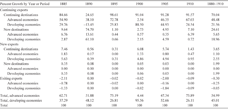
Table 2 provides these decompositions in percentage terms for each five year interval and the three decades as a whole. We group the decompositions by good type (i.e., continuing, new, exiting) and within each of these by destination (i.e., continuing, new) and economy type (i.e., advanced, developing).Footnote ¹⁰ The final column of Table 2 shows that expansion of exports of products already exported in 1880 to the same trade partners in that year and for the entire 30 year period (i.e., intensive margin) account for 70 percent of growth, with exiting goods of any type accounting for less than 0.3 percent. The remaining growth can be separated along the two extensive margins of new goods (3.7 percent), new destinations (24.6 percent), or both (2 percent). Alternatively, for new exports over the entire period to both new and continuing trade partners, their contribution is approximately 5.6 percent of export growth; for new destinations regardless of export type, it is about 26.6 percent. These breakdowns indicate that for extensive growth, entry into new markets was significantly more important than the export of new goods.Footnote ¹¹

For both the new destinations and new goods margins, developing economies account for more than four times that share in export growth than advanced economies. For new destinations we observe growth of 20.94 percent (18.96 from continuing products and 1.99 from new products) versus 5.65 percent. For new goods, the values are 4.54 (2.55 from destinations already served by other goods and 1.99 to entirely new destinations) versus 1.10. Overall growth in total exports in this period is explained nearly evenly by the two groups of economies, although there is substantial volatility in the five year intervals. Trade with developing economies grew 38 times in value compared to the 12-fold increase with advanced economies. Since exports to poorer countries were smaller in value in both 1880 and 1910 compared to wealthier ones, the share of overall growth explained by the former is smaller. Nonetheless, these decompositions support our interpretation that, on the margin, new goods enjoyed easier access in developing economies even if the new goods margin contributes relatively little to overall export growth. This is especially remarkable given Japan’s lack of tariff autonomy for most of the period and European dominance in Asian trade before WWI.

The size of these margins and overall results correspond closely to the quantitative magnitudes in Evenett and Venables (Reference Evenett and Venables2002) studying a sample from 1970 to 1997. They find that for all trade flows in their sample 78 percent of trade growth was in continuing goods to continuing countries, the share of continuing goods to new partners made up 21 percent of growth, new products accounted for 1.7 percent, and exit was negligible. Excluding the extensive margin by new trade partnerships, the fraction of overall trade explained by continuing goods is 94.6 percent in our analysis, lower than the 98 percent found in Evenett and Venables (Reference Evenett and Venables2002).

It should also be noted that the margins calculated for our sample are for the universe of products and trade partners over the entire three decades. Country-level analysis indicates different trajectories. The extensive margin in terms of new goods mattered the most for Germany (48 percent) and Korea (23 percent), while for China and the United States, new goods accounted for 6.5 and 2 percent, respectively. Likewise, decompositions for the shorter five-year intervals show that the intensive margin is responsible for 85 to 90 percent of average export growth for each period on average. One notable exception is in 1890, when Hong Kong and British India appear as new destinations and the intensive margin declines substantially. Given these deviations by interval or country, the decomposition for the three decades as a whole across all trade partners is more representative of the evolution of Japanese exports during the first wave of globalization.

First Market Entry: Determinants of Extensive Growth

Having established that extensive growth into new destinations played an important role in explaining Japanese export patterns from 1880 and 1910, we explore more systematically the timing and determinants of market entry. In the nineteenth century, as now, trade costs were a key determinant of trade flows (Jacks, Meissner, and Novy Reference Jacks, Meissner and Novy2011; Huberman, Meissner, and Oosterlinck Reference Huberman, Meissner and Oosterlinck2017). Trade flows and the particular products shipped were impeded not only by high and selective tariff rates under various treaty provisions, but also by distance that determined transportation costs and information about market opportunities.

Shipping costs at this time accounted for roughly 2 to 5 percent of the value of the good and were generally declining due to improvements in shipping capacity and steamship innovations. Market intelligence was effective and depended on the networks of sales agents. The density and reliability of these networks also varied greatly by industry and location (Marrison, Broadberry, and Leunig Reference Marrison, Broadberry and Leunig2007). In the late nineteenth century, the diplomatic and consular network extended itself significantly, facilitating transactions by cutting red-tape (e.g., foreign consuls in the sending country) with consular staff reporting back to the home country about market opportunities. Much of the cost of accumulating up-to-date market intelligence could be considered a fixed market entry cost since these costs varied little by the size or value of shipments. These fixed costs might help explain why some destinations and products failed to receive Japanese exports. At the same time, the decision to enter a market or to send a good depends on the capacity of the market to generate revenue, and factors at the product, industry, and firm levels could influence revenues given fixed costs. Finally, other costs like trade finance, credit constraints, consumer preferences, insurance and storage have been cited in the literature and in contemporary treatments of trade relations.

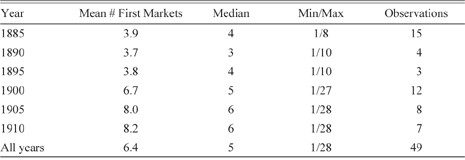
In our sample, the mean number of destinations when a product is first shipped is 6.4 and the median is 5. Summary statistics for each quinquennial period are also shown in Table 3. The mean, median, and maximum number of first markets entered increased over time, and the average grew faster than the median.

Table 3

Summary Statistics for First Market Entry, 1880–1910

Note: A first market is defined as a market where a product has positive exports in the first year the product appears in the trade data.

Source: Authors’ calculations.

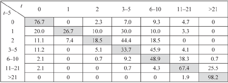
To explore the dynamics of destination market entry (and exit), we calculate a transition matrix for the number of markets served in a base year and then in the following period using the population of products with positive exports in a given year. In Table 4, the rows in the transition matrix break the initial period number of destinations into 0, 1, 2, 3–5, 6–10, 11–21, and more than 21 destinations. Columns in this table show the number of destinations five years later. The frequencies or shares of goods in each entry can be interpreted as transition probabilities from the initial state to the state in the following period.

Table 4

Transition Matrix for Number of Destinations

Note: Row headings are for the number of destinations in year t-5 and column headings are for those served in year t for a given product. A period is a year in these data. The matrix diagonal gives the percentage of goods with no change in number of destinations served between t − 5 and t, while the upper right (lower left) cells give the percentages of increased (decreased) market penetration. Source: Authors’ calculations.

We observe that there is some persistence in the number of markets over time, as indicated by the large positive probabilities along the matrix diagonal. Comparing the upper right and lower left halves of the matrix bisected by the diagonal, the probabilities of expanding into new markets over time are much higher than exiting existing markets. Once a product is shipped to between six and ten destinations, the probability of a move to the lower bins (i.e., moving to less than six destinations) is cut by one-third to one-half. This suggests that product/industry level “ability” to export was important or there were economies of scale in exporting. Furthermore, we find evidence of interesting dynamics based on sequencing: products starting in one market had a probability of more than 50 percent of finding new markets in the subsequent period, and for the most successful products (i.e., those with 11 or more markets) the probability of staying in the current range or expanding was higher than 90 percent. Especially successful products, such as those exported to nearly all active partners, maintained at least 21 markets or more with a probability of 98 percent.

Below the threshold of six markets, there is a non-negligible probability of dropping the number of destinations. For example, products shipped to one market in the previous period have a 20 percent chance of exiting. Products shipped to two destinations have an 11 percent chance of exiting completely or a 7 percent chance of losing one market in the next period. Once a product secured a place in more than six markets, the probability of a decline below six markets decreases significantly. All of this is consistent with the idea that Japanese products, in trying to break into international markets, learned something about their export capabilities on global markets that enabled them to ship to new markets and once established rarely left.

These findings are supported by regression analysis that includes additional covariates for trade costs at the country level and controls for market characteristics. With regard to first market entry for an export that becomes active in any year between 1885 and 1910, we model the first entry decision at the country-product-year level with a pooled logit model. A product-destination-year observation receives a one in the first year this product is active and for each country where a product launches for the first time.Footnote ¹² All other destinations which are not served for this particular product in the first year of exporting and in all years prior to the initial year of exports receive a zero. After entering, a product is dropped from the sample in subsequent years. Specifically, we estimate the probability, π, that a destination country d is in the set of first destinations for product p in year t as:

$\pi _{pdt}^{FM} = F({\tau _{dt}}{\beta _0} + {X_{dt}}{\beta _1} + {\delta _t}).$

We break down the determinants of first market (FM) entry into two categories. The first category of determinants, τ, is trade costs with a vector of coefficients, β ₀. We include product invariant proxies for trade costs such as distance, MFN treaty status, pegged exchange rate with the destination, diplomatic representation of the destination in Japan and that of Japan abroad, and whether the destination was the colony of another country. Such variables, as already stated, determine the amount of revenue generated in a destination market and some proxy for the fixed costs of market entry.

The second category, X, with the associated vector of coefficients, β ₁, could be described as destination-market or demand factors. We include two variables related to size: the logs of the sum of pair-GDP and similarity of total GDP of the destination and Japan (i.e., log of the product of the share of GDP relative to total GDP of the dyad), respectively. A third variable, the log of the absolute difference in GDP per capita between Japan and its export destination, accounts for whether Japan was more likely to enter into markets where the demand structure varied from Japan’s. If so, we expect a positive partial effect; otherwise, a negative coefficient would indicate that Japan traded mainly with countries at a similar level of development. Staffan Linder (Reference Linder1961) hypothesized that richer countries would specialize in high quality goods and rich country consumers would have higher demand for such goods. Countries at similar levels of development would then have more trade, ceteris paribus.

As discussed in Juan Carlos Hallak (Reference Hallak2006), a negative coefficient on per capita income differences would be consistent with the Linder hypothesis, suggesting that Japan was increasingly exporting higher quality goods to high income destinations as its economic growth proceeded at a rate faster than the world average growth rate. This would also correspond to a test of Christopher Howe’s (Reference Howe1996) observation that Japan followed a strategy of exporting low quality goods to low income markets even as it embarked onto a path of modern economic growth. Other covariates relating to demand conditions include the number of other products shipped to this destination in the previous period and the average growth rate of the value of other products between the current year and five years ago to this destination. Finally, we include time and region dummy variables with the year 1880 and Asia being the omitted categories, respectively.

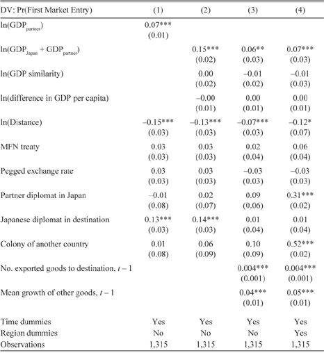
As shown in Table 5, gravity model predictions hold in our regression results, with market size (i.e., partner GDP or the combination of Japan and partner incomes) consistently associated with greater export value and distance associated with less exporting. A doubling of market size is associated with an increased probability of being in the set of first markets of between 7 and 15 percentage points; similarly lower probabilities obtain for markets twice as distant. For the former, one interpretation is that rather than trying to match preferences it appears that Japanese products first tested themselves in the largest markets both rich (e.g., United Kingdom) and poor (e.g., China).

Table 5

Logit Regression Results for First Market Entry

^* = Significant at the 10 percent level.

^** = Significant at the 5 percent level.

^*** = Significant at the 1 percent level.

Dependent variable is equal to one when a country is in the set of countries in the initial year a product appears in the data and zero if the country is not in this set. Average partial effects are shown. Robust standard errors clustered at the destination-good level are in parentheses. Method of estimation is logit maximum likelihood.

Source: Authors’ calculations.

Neither similarity in overall size of GDP, nor GDP per capita differences, is a significant correlate of market entry, which may be due to a scale effect where larger markets (regardless of individual income levels) can support higher sales volume for a fixed entry cost. Alternatively, it could be that the fixed costs of entry were lower in these markets. Other trade costs such as most favored nation treaties and fixed exchange rates, are not statistically significant, which may be due to reshipment of exports to third parties after reaching the first (and only documented) destinations like London or Marseilles and Japan’s change from fiat currency to silver and then to gold over this period. Variables for product-specific determinants are inconsistent in predicting market entry as well: market intelligence via diplomatic representation varies both in sign and significance depending on the specification. Colonial status is statistically significant only in the last specification that includes both time and region dummies, but not without the latter.

More interesting are the lagged terms for export activity, which are positive and statistically significant when included. A destination that had received either more types or volume of Japanese exports was more likely to see additional entry of new products, suggesting that market presence is both persistent and augmenting for new product launches. Although the magnitudes are small, given the average number of products received by a given destination and the sheer volume of export growth over this period, neither is negligible. These forces are important even after controlling for period fixed effects, which we do throughout, the overall size of the market, and the geographic region.

General Market Entry Analysis of Extensive Growth

To extend this analysis to subsequent market entry beyond first markets, we again use a pooled logit model to explain further entry at the product-destination-year level. We assign a one to each country-product-year observation if the product has already previously entered into at least one market in the world in the previous period and then entered a particular destination in a given year. The destination-product pair observation drops from our sample after the year of entry. Furthermore, once a product is active in at least one destination country, each country-product observation where no positive sales have been previously recorded becomes “at risk.” We assign these observations a zero. We estimate the probability of entry, $\pi _{pdt}^{SM}$ , for product p, in destination country d, in year t, using a pooled logit model as follows:

$\pi _{pdt}^{SM} = F({\tau _{dt}}{\beta _0} + {X_{dt}}{\beta _1} + {X_{pt}}{\beta _2} + {\delta _t}).$

For the market entry decision, we include a vector of trade cost controls, τ _dt , a vector of destination controls, X_dt , and a third category of determinants, X_pt , that are time-varying and product specific. We include the change in the logarithm of a product’s sales to all other markets between the current year and five years earlier. If a product is growing strongly in general then it might be expected to have success in the next market. We also include dummy variables for the number of destinations for the product in the previous period, grouped using the same bins as in the transition matrix of Table 4 (i.e., 2, 3–5, 6–10, 11–21, and more than 21 markets). Finally, we include a full set of region and year fixed effects.

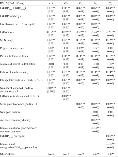
Table 6 reports our results. Similar to our first entry results, size (e.g., sum of Japan-trade partner GDPs) and distance both matter, although the former has less predictive power and the latter more. The elasticity of the probability of entry with respect to size is one-third to one-half the magnitude of the elasticity with respect to a decline in distance. The average partial effect in column 1 of Table 6 for size is 0.03 while for a 1 percent drop in bilateral distance it is 0.15. The partial effects of differences in income per capita, unlike the earlier results on first entry, are now consistently positive and statistically significant. These results suggest that once a product had been “tested” in a large international market, it was more likely to expand entry into countries that are dissimilar from Japan in terms of GDP per capita. As Japan was by international standards a poor, but fast-growing economy throughout this period, it seemed able to gain new markets for particular products in countries that were growing relatively more slowly—ostensibly where demand may have been more favorable.

Table 6

Logit Regression Results for all Market Entry

^* = Significant at the 10 percent level.

^** = Significant at the 5 percent level.

^*** = Significant at the 1 percent level.

Dependent variable equals one when a product is already exported to at least one country in the sample and is first exported to the given country and zero if the product has not yet experienced positive exports. The sample excludes the first destination countries when a product first appears in the data set. Average partial effects are shown. Robust standard errors clustered at the destination-good level are in parentheses. Method of estimation is logit maximum likelihood. Dummy variables for time, region, and lagged number of markets are included but not reported.

Source: Authors’ calculations.

Trade costs like MFN treaty status and pegged exchange rates also become positive and significant, with the magnitude of the partial effect of an MFN exceeding that of a pegged exchange rate by an order of magnitude. MFN treaties are associated with a rise in the probability of entry of about 12 percentage points compared to about 2 percentage points for a fixed exchange rate. It is surprising to see that if a destination is the colony of another country a product is more likely to enter. This average partial effect may be due to collinearity with the region fixed effects and diplomatic representation as large nations with empires were more likely to have diplomatic representation in Japan.

As from the earlier results in Table 5, product specific factors are clearly consistent correlates across all columns. Existing market presence and growth in the previous five years to other markets are positive and significant. For example, a doubling in the growth of sales is associated with a roughly 2 percentage point increase in the likelihood of entry. The mean rise in sales in our sample is 0.59 log points with a median of 0.52, a 75th percentile of 1.18 and a 95th percentile of 2.8. The full sample likelihood of entry is 0.08 (i.e., 8 percent). The lagged number of markets served in the previous period by a product is positive as well. The average partial effect, which is not shown in the table to conserve on space, is larger in magnitude as the number of markets increases. For example, in the first column’s specification, products serving two markets have a 0.02 (i.e., a 2 percentage point) higher likelihood of entry than for one market. For products serving 11 to 21 markets or more than 21 markets, the increase is very sizeable in economic terms, raising the probability by 17 and 38 percentage points, respectively.

Highlighting the possibility that product entry is more likely in markets that are geographically proximate to other extant markets with active exports, we include a variable for lagged distance to Japan’s nearest active market for a given good in column 2. We also use another metric of similarity, namely proximity in product space. We create a variable equal to the lagged value-weighted average of the SITC codes of active exports to a market. We then take the log of the absolute value of the difference between the SITC code for a product not yet entered and this weighted average.Footnote ¹³ The goal here is to test for demand complementarities in the sense that products related in the product space are more likely to enter when similar exports are already being exported to a given market. For both these variables, we find that proximity has a small, but statistically significant association with entry with the expected signs: distance to the closest active market is negatively related to entry while growth in related goods is positively related. The last two columns include an indicator variable for a new good, and the probability of entry for a new good is lower whether interacted with the advanced economy dummy or trade partner per capita income. This evidence is consistent with the observation in Howe (Reference Howe1996) that Japan was increasingly competitive in poorer markets by tailoring its products to suit their preferences and reducing trade costs, even as the country continued to expand trade with its existing and wealthier partners.

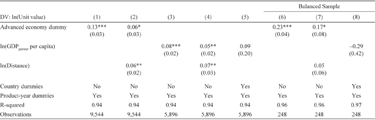
To test whether quality differences influenced Japanese export expansion, we use product unit values by destination market. The rationale is based on the Linder hypothesis that richer (poorer) countries demand higher (lower) quality for the same good, which we approximate with price. Table 7 presents results from linear regressions of the following form:

$\ln ({\rm{Unit\,Value}}_{pdt}) = {\beta _1}\ln ({\rm{GDP\,per\,capit}}{{\rm{a}}_{dt}}) + {\beta _2}\ln ({\rm{distanc}}{{\rm{e}}_d}) + {u_{pt}} + {\varepsilon _{pdt}},$

Table 7

Linear Regression Results for Export Unit Value, 1880–1910

^* = Significant at the 10 percent level.

^** = Significant at the 5 percent level.

^*** = Significant at the 1 percent level.

Robust standard errors clustered at the destination-good level are in parentheses. Method of estimation is OLS. Product unit values are calculated using total exports for each exported product by country and total quantity. Advanced economies include United States, United Kingdom, France, Luxembourg, Italy, Germany, Australia, Holland, Belgium, Denmark, Sweden, and Norway; remaining countries are designated as developing. The balanced sample in columns 6 to 8 comprises products continuously exported throughout the period and exported to at least one advanced and one developing economy.

Source: Authors’ calculations.

where the dependent variable is the log of the unit value. Our independent variables include either an advanced economy indicator or the log of GDP per capita of the destination market; the log of shipping route distance from Japan or country dummy variables; a set of product-year indicators u_pt ; and an error term ε_pdt . Product-year indicators control for level differences in unit values across products as well as product-specific supply shocks or global demand shocks to the particular Japanese good.

Estimates in the first five columns, which use either the advanced economy dummy or partner GDP per capita, show that wealthier destinations are positively associated with the unit values. In column 2, when we control for one major determinant of trade costs, distance, the coefficient on the advanced indicator falls from 0.13 to 0.06, suggesting that part of the reason richer countries have higher unit values is that they are more distant in our sample. The distance coefficient is positive in this specification, which is a standard result when some fraction of trade costs is “specific,” implying economies of scale in shipping (compare Table 6 in Bernard, Jensen, and Redding Reference Bernard, Jensen and Redding2007). Richer countries may import higher unit value goods from Japan, but this is largely because of the nature of trade costs.

When we control for many unobservable trade costs and destination specific demand factors with country fixed effects, GDP per capita is no longer significant (column 5). In columns 6 through 8 we control for changing composition of goods by running these regressions only for the panel of goods which are shipped in all seven quinquennial periods and have at least one advanced and one developing destination. Results from this balanced sample are qualitatively the same as those in the preceding columns. In other words, since higher priced goods are not associated with wealthier partners after country fixed effects are included, we cannot rule out that trade costs play a more important role in explaining destination prices rather than quality.Footnote ¹⁴

Using unit values as a proxy for quality may be problematic when investigating product quality, so we examine Indian imports of four broad product categories from seven exporting countries: Belgium, China, France, Great Britain, Hong Kong, Italy, and Japan. The products are “cotton twist and yarn,” “cotton piece goods white (bleached),” “cotton piece goods, colored, printed, or dyed,” and “silk piece goods” and were imported between 1891 and 1907. Results from our linear regression (not shown) with quantity as the dependent variable and the covariates of unit price, a time trend, and country and product fixed effects indicate that increased Japanese market share was not associated with price differences. Separate specifications using year indicators and their interaction with Japan’s country indicator show similar results. We interpret these findings as consistent with increased Japanese exports due to a decline in trade costs, especially the types of fixed trade costs that depend on product volume or weight.

Market Exit: Analysis of Extensive Growth

Finally, we analyze market exit for Japanese exports, which we have shown earlier played a smaller role during our period. In our sample there are 269 cases of “permanent exit” compared to 1,703 entrances and 394 first market observations.Footnote ¹⁵ Permanent exit is defined for a good when exports of a product-country pair in the previous period were non-zero but are zero in the current year and every following year for that product-country pair. We restrict attention to the period 1880 to 1905 since we did not collect data post-1910. There are 393 more observations where a product temporarily ceases to be sold in a market. We restrict attention to the cases of permanent exit from a market since temporary exits may reflect transitory factors, which are of less interest in explaining the long-run transformation of Japanese exports.

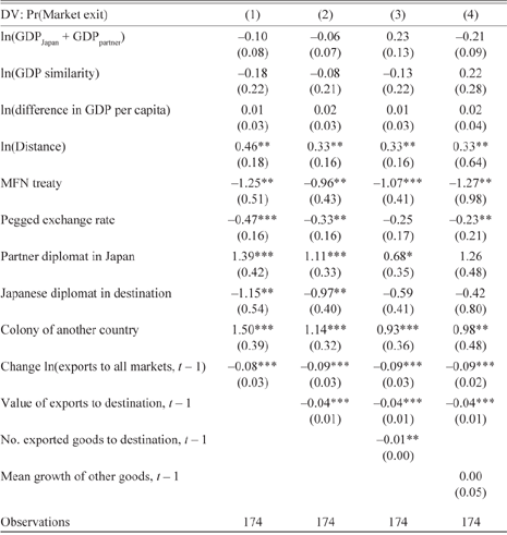
We use the logit regression model specifications from Table 6 to explore the determinants of exit; the dependent variable is one in the year when a product-country pair experiences a permanent exit. As before, we control for trade costs, market demand, and product specific factors. Since there are so few exits, many indicators cannot be precisely estimated or need to be dropped completely. This is the case for the region dummies and the indicators for exports to two markets or greater than 21 markets. Since a product has a zero value in the year it exits, we cannot include growth of exports of this product between the current year and the previous period. Instead we include the level of exports in the previous period to a market by a product.

Our results, shown in Table 8, indicate that rising distance is associated with a higher likelihood of exit, which is consistent with our observation that European trade shares declined over time in favor of Japan’s Asian neighbors. The only other trade cost proxies that are statistically significant are MFN treaty status, the fixed exchange rate indicator and the colony indicator. Both the average partial effects of MFN treaty status and fixed exchange rates are negative and statistically significant, which we interpret as offsetting the distance effect. Colonies were difficult to maintain according to our results here.

Table 8

Logit Regression Results for Market Exit

^* = Significant at the 10 percent level.

^** = Significant at the 5 percent level.

^*** = Significant at the 1 percent level.

Average partial effects are shown. Robust standard errors clustered at the destination-good level are in parentheses. Method of estimation is logit maximum likelihood. Dummy variables for time, region, and lagged number of markets are included but not reported.

Source: Authors’ calculations.

Market-specific factors are not consistently statistically significant. While market size and similarity in size played strong roles in explaining first entry and subsequent entry into other markets, they play no significant role for exit. This corresponds with the view that fixed costs matter. In large markets, entry depends on covering fixed costs but for exit a similar logic does not apply since it is free. We find that exit is less likely when the number of goods sold in a market rises. Moving from selling ten to 50 goods to a market would decrease the probability of exit by nearly 40 percentage points. At the same time, average growth of all other products is not a significant determinant.

Product specific factors are also important. We find that when the growth of exports to the rest of the world of this product is high, a product is less likely to exit a market. Large levels of exports to a country in the previous period are also associated with lower exit probabilities, while the number of markets in which the product has sales does not seem to matter. None of the indicators for number of markets is individually statistically significant. Although expanding the number of markets seems to be a key determinant of entry, exit does not depend on the number of markets as much as strong growth of sales along the intensive margin. Once again, this is compatible with the notion that fixed costs are important for entry. Moreover, expansion of the intensive margin seems to depend on the past insofar as past success correlates with product-level unobservables.

Conclusions

Between its dramatic liberalization in the 1850s and the first decades of the twentieth century, Japan traversed a path of unprecedented economic convergence to leading industrial economies in the West. Its integration with world markets provided it not only with significant gains from trade (Bernhofen and Brown Reference Bernhofen and Brown2005), but also promoted institutional, structural, and technological change (Basco and Tang Reference Basco and Tang2017; Braguinsky, Ohyama, Okazaki, and Syverson Reference Braguinsky, Ohyama, Okazaki and Syverson2015; Morck and Nakamura Reference Morck and Nakamura2007; Nicholas Reference Nicholas2011; Perkins and Tang Reference Perkins and Tang2017; Tang Reference Tang2016; Tang Reference Tang2017). How did trade interact with domestic production, and are there discernable patterns to Japanese export success?

In this article, we decomposed Japanese export growth by margin type and found that extensive growth in markets and goods accounted for nearly one-third of total export growth. Rather than merely persisting in exporting the same goods as it did in 1870 or 1880, Japan diversified its portfolio of exports and moved up the value added chain. In particular, Japan progressively moved from being an exporter of raw materials in which it had a comparative advantage to an exporter of cotton thread, cotton textiles, and other more elaborate manufactured goods.

Japan also initially exported its traditional goods to rich countries and a handful of near neighbors. Between 1880 and 1910 its focus shifted strongly to less developed economies in the Asian region and away from the so-called advanced economies, and this margin of extensive growth contributed much more to growth than the export of new goods. While Japan’s comparative advantage may have changed over time, our results show that trade costs and market demand patterns also mattered. These changes in destinations and exported products tell us much about the Japanese economic experience of the late nineteenth century and is comparable to what modern day emerging economies have achieved in the second wave of globalization. At the same time, intensive growth remained important, and this margin for Japan is roughly similar to Belgium’s, the only other country for which comparable data have been digitized and analyzed in this period (Huberman, Meissner, and Oosterlinck Reference Huberman, Meissner and Oosterlinck2017).

Based on the importance of extensive market growth, we further explored whether trade costs, market specific forces, and product specific factors mattered for entry and exit of Japanese products and derived some stylized facts. First, gravity holds: market entry depended largely on market size and proximity. Better information about markets and market size also appear to mitigate the fixed costs of exporting and these large markets were good places to test the potential of expansion into other markets. Once established, exports increased intensively and extensively, with tried products fanning out into other markets. As Japan’s economy converged toward the leaders, it became more likely to enter and to stay active in relatively poor markets. The growth of exports in new products appears to have been the outcome of declining trade costs more than matching quality to the destination. In other words, our evidence does not conform with the idea that export growth in Japan focused on providing low-cost, low quality goods in low-income countries. Moreover, the bulk of export growth remained in the intensive margin, which meant that even as Japan expanded into new markets and with new goods, it kept exporting products that it had produced since the beginning of the period. This suggests the country was able to increase its range of partners and goods even as it remained competitive in existing markets without discarding products that powered its industrialization drive.

All of these results are established using a new disaggregated trade dataset of which we are the first to analyze. While they echo patterns seen in other countries in the period and in modern times, there are some differences. First, Japan lacked tariff autonomy and thus was constrained in terms of trade policy. This contrasts with the experiences of countries in recent decades, those of the leading countries of the nineteenth century, and Latin America where trade policies were usually autonomous decisions that reflected local social and political preferences. Japan was also geographically isolated in the period compared to the average European economy and had a relatively small domestic market compared to the United States. That said, Japan had some early advantages due to its factor endowments and relative proximity to the two large and poor markets of China and India. Our analysis suggests that compared to western producers Japan was able to more easily capitalize on the size of these neighbors to learn how to export higher value-added goods. Further historical work using similar data sets in other countries is on the cusp of being developed and studied. Such research will allow us to make finer and more careful comparisons between Japan and the rest of the world as well as improve our understanding of how both developed and developing markets integrated over time.