

Implications
Present results provided a clear insight into the population structure and evolutionary history of the Frizarta dairy sheep. First, they are in accordance with historic reports suggesting the extensive use of East Friesian (EF) rams during the breed’s formation. Second, the breed displays low linkage disequilibrium (LD) levels similar to outbred populations. These LD levels render the use of a denser than the 50k single nucleotide polymorphism (SNP) more beneficial when performing genome wide association studies (GWAS) in the breed. The most recent effective population size was estimated relatively low probably due to recent inbreeding.
Introduction
The Frizarta dairy sheep is one of the most important Greek breeds. It is kept in the western part of Greece and more specifically in the Arta and Agrinio districts and it currently numbers 11 000 officially registered ewes, dispersed in 87 herds (Center of Animal Genetic Improvement of Athens, April 2016, Personal communication). It is a synthetic breed formed by extensive mating of local ewes with EF rams during years 1963 to 1967 and 1968 to 1982. Since then, the breed has been successfully adapted to the local climate of the area with mild winters, high rainfall and high relative humidity. The average 190 days milk yield, fat content, protein content, lactose content and litter size are 256 kg, 6.28%, 5.61%, 4.54% and 1.6% lambs per ewe and year, respectively (Cooperative of the Agricultural and Livestock Union of Western Greece (ALUWG)). Recently, ALUWG has undertaken initiatives toward the application of a modern selection program, including genotyping of animals with the 50k SNP array to assess the efficiency of alternative selection methods such as genomic selection. Application of the 50k SNP array has also allowed for carrying out GWAS in the breed (e.g. Kominakis et al., submitted).
In the current study, we estimated various population measures and parameters in an attempt to investigate the population structure and the evolutionary history of the Frizarta dairy sheep. Current results are expected to facilitate the design of more efficient selection programs and to improve genetic management of the breed.
Material and methods
Single nucleotide polymorphism genotyping and quality control criteria
A total of 524 dairy ewes of the Frizarta breed were included in this study. These ewes were randomly selected from seven herds of the ALUWG. Ewes are kept under an intense production system, with standardized conditions and feeding regime. Deoxyribonucleic acid was extracted using the NucleoSpin Blood kit (Macherey-Nagel, Duren, Germany). Sample genotyping with the OvineSNP50 BeadChip (Illumina, San Diego, USA) was performed by Neogen Europe Ltd (Ayr, Scotland, UK). From the 524 original samples, only one sample could not be genotyped. We performed quality control (QC) of the remaining genotypes in two stages, first on an ‘individual’ and second on a ‘marker’ basis. First, samples were removed if they had (i) call rate <0.95 and (ii) overall autosomal heterozygosity rate outside the 1.3 inter-quartile range (IQR=0.345 to 0.391). Using these criteria, the number of available animals (samples) was reduced to 503. Second, marker QC was based on the following criteria: (i) call rate (⩾0.95), (ii) Fisher’s Hardy–Weinberg equilibrium P<0.0001), (iii) minor allele frequency (MAF) >0.20. A relatively high threshold for MAF was chosen as LD is preferably estimated using high-frequency polymorphisms (Reich et al., Reference Reich, Cargili, Boik, Ireland, Sabeti, Richter, Lavery, Kouyoumjian, Farhadian, Ward and Lander2001; Qanbari et al., Reference Qanbari, Pimentel, Tetens, Thaller, Lichtner, Sharifi and Simianer2010). Following the above criteria, a number n=17 115 SNPs were dropped. Finally, only SNPs located on the autosomes and only mapped SNPs were considered resulting in a number of n=1819 SNPs excluded. From the originally available number of SNPs (n=53 998), the number of SNPs retained for further analysis was 35 058. Marker QC was performed with the SNP & Variation Suite software version 8.6.0 Win64 released on 18th October 2016 (Golden Helix Inc., Bozeman, USA).
Estimation of linkage disequilibrium
Linkage disequilibrium levels for all pair wise combinations of SNPs as well as between adjacent SNPs were estimated using r 2 (Hill and Robertson, Reference Hill and Robertson1968) and |Dʹ| (Lewontin, Reference Lewontin1964) measures. Both Dʹ and r 2 range from 0 to 1. Dʹ represents a more accurate statistic for estimating recombination differences, whereas the r 2 statistic summarizes both recombinational and mutational history of a population. Dʹ has been shown to be inflated by small sample sizes and low allele frequency, whereas the bias due to allele frequency is considerably smaller in r 2 than that in Dʹ (Ardlie et al., Reference Ardlie, Kruglyak and Seielstad2002). Both LD estimates were obtained with the SNP & Variation Suite program (Golden Helix Inc., 2016). The two LD measures were also estimated in a sample of EF animals (n=48) that were obtained from the publicly available data of the Sheep HapMap project (http://www.sheephapmap.org/hapmap.php).
Linkage disequilibrium decay rates by chromosome
The decline rate of LD with inter-marker distance (in kb) was estimated per chromosome by fitting the following equation:
 $$y_{{ij}} \, {\equals}\, {1 \over {\left( {1{\plus}4\beta _{j} d_{{ij}} } \right)}}{\plus}e_{{ij}} $$
where y
ij
is the estimated
 $$\hat{r}^{2} $$
after correcting for sampling error
 $\hat{r}^{2 \prime } \, {\equals}\, \hat{r}^{2} {\minus}E ( {\hat{r}^{2} _{{{\rm sample}}} } )$
. Hill and Robertson (Reference Hill and Robertson1968) suggested that
 $$\hat{r}^{2\prime } '\, {\equals}\, {{( {\hat{r}^{2} {\minus}1/N )} / {( {1{\minus}{\raise0.7ex\hbox{$1$} \!\mathord{\left/ {\vphantom {1 N}}\right.\kern-\nulldelimiterspace}\!\lower0.7ex\hbox{$N$}}} \right)}}$$
with N twice the number of sampled individuals whereas Weir and Hill (1980) proposed
 $$\hat{r}^{2\prime } '\, {\equals}\, \hat{r}^{2} {\minus}{\raise0.7ex\hbox{$1$} \!\mathord{\left/ {\vphantom {1 N}}\right.\kern-\nulldelimiterspace}\!\lower0.7ex\hbox{$N$}}$$
with N the number of sampled individuals. Waples (2006) proposed
 $E ( {\hat{r}^{2} _{{{\rm sample}}} } )\, {\equals}\, \left[ {{1 \over N}{\plus}{{3.19} \over {N^{2} }}} \right]$
which approximates the correction factor of Weir and Hill when ignoring the
 $${{3.19} \over {N^{2} }}$$
term for relatively large N (sampled individuals). Finally, Sved et al. (2013) suggested
 $E ( {\hat{r}^{2} _{{{\rm sample}}} } )\, {\equals}\, 1{\minus}{1 \over {\left( {2N{\minus}1} \right)^{2} }}$
. As a relatively high number of samples were available in the present study, correction of the
 $$\hat{r}^{2} $$
estimates was performed using the Weir and Hill (1980) method with N=503. Furthermore, d
ij
is the inter-marker distance (in kb) for marker pair i at chromosome j, β
j
is the coefficient that describes the decline rate of LD with distance (large values indicate low extent of LD) for chromosome j, and e
ij
is a random residual with e
ij
~(0,s
2). A maximum inter-marker distance of 40 000 kb was considered here. This analysis was carried out with procedure NLMIXED in SAS (2014) by using a random sample of 802 760 pairs of markers (out of 16 055 202 available in total) that had no negative or 0 values (because of correction for sample size).
Estimation of historical population size
Assuming a linear population growth, the historic effective population size (N e ) was estimated as (Hill, Reference Hill1981; Hayes et al., Reference Hayes, Visscher, McPartlan and Goddard2003)
 $$N_{{e(t)}} \, {\equals}\, {{1{\minus}\hat{r}^{2 \prime} } \over {4c\hat{r}^{2 \prime} }}$$
where N
e(t) is the effective population size t generations ago, c is length of the chromosomal fragment in morgans (Hayes et al., Reference Hayes, Visscher, McPartlan and Goddard2003) with t=1/(2c), and
 $$\hat{r}^{2\prime} $$
the adjusted
 $$\hat{r}^{2} $$
for sample size as previously described. Assuming an average generation interval of 3.75 years, the estimation of N
e
was performed at three distinct time points, namely at the beginning of the population formation (year 1963, 13.89 generations ago), the end (year 1981, 9.26 generations) and most recently that is one generation ago (year 2012) using both single chromosome and pooled (all chromosomes) data. The physical length of chromosomal fragments (in kb) used to estimate average
 $$\hat{r}^{2} $$
for each of the three time points was determined from the equation t=1/(2c) assuming an average genomic recombination rate of 1.2 cM/Mb for the species (Dumont and Payseur, Reference Dumont and Payseur2008). Thus, estimation of N
e
for the years 2012, 1981 and 1963 was based on average
 $$\hat{r}^{2} $$
values from 3000±100, 4500±100 and 40 000±500 kb fragments, respectively.
Multidimensional scaling analysis and Heatmap of genetic similarity
A multidimensional scaling (MDS) analysis was conducted to detect possible population stratification. First, a matrix of identity by state values, also known as the genomic relationship matrix (GRM), was calculated between all pairs of the 503 individuals using genotypes of the 35 058 SNPs. Multidimensional scaling analysis was performed on the distance matrix derived from the matrix of the kinship values and possible stratification was resolved using the two dimensions. This analysis was performed by procedure MDS in SAS (2014). Finally, a heat map along with k-means clustering of the animals’ kinship values was performed using the GENE-E matrix visualization and analysis platform (https://software.broadinstitute.org/GENE-E/).
Estimation of FST
The Wright’s fixation index F ST , was used as a measure of genetic divergence of the seven herds (Hartl and Clark, Reference Hartl and Clark2007):
 $$F_{{ST}} \, {\equals}\, {{\sigma _{S}^{2} } \over {\sigma _{{\rm T}}^{2} }}\, {\equals}\, {{\sigma _{S}^{2} } \over {\bar{p}\left( {1{\minus}\bar{p}} \right)}}$$
where,
 $\sigma _{S}^{2} $
is the variance in the frequency of the allele between different subpopulations (herds), weighted by the sizes of the subpopulations,
 $\sigma _{{\rm T}}^{2} $
is variance of the allelic state in the total population and
 $\bar{p}$
is average frequency of an allele in the total population. F
ST
values can range from 0 (no genetic divergence between the herds) to 1 (complete isolation of the herds). A matrix of the herd F
ST
values was then constructed and this was further subjected to MDS analysis. This analysis was performed by procedure MDS in SAS (2014). Genetic differentiation between herds was assessed by visual inspection of the two-dimensional plots. Furthermore, a plot of F
ST
values by herds’ geographical distances was also created in an attempt to investigate for possible gene flow between herds.
Estimation of migration rate
Assuming equilibrium between gene flow and drift, gene flow
 $\hat{M}\, {\equals}\, N_{e} m$
(Slatkin, 1993) was approximately estimated by solving the classical Wright’s formula (1951) for the N
e
m term:
 $$F_{{ST}} \,\approx\,{1 \over {1{\plus}4N_{e} m}}\to\hat{M}\, {\equals}\, N_{e} m\,\approx\,{1 \over 4}\left[ {{1 \over {F_{{ST}} }}{\minus}1} \right]$$
Here, F
ST
was approximately estimated using the formula of Nei and Chakravarti (Reference Nei and Chakravarti1977)
 $$F_{{ST}} \,\approx\,1{\minus}{\rm e}^{{{\minus}t\!/\!\left( {2N_{e} } \right)}} $$
and N
e
estimates obtained from formula (1). N
e
m is the number of individuals in the population that are new immigrants in any generation and m is the migration rate, that is the fraction of individuals in the population that are immigrants. Here, the Wright’s ‘Continent-Island’ model (Wright 1931 and 1940) was presumed rather than the ‘island model’, assuming that F
ST
among herds is a result of gene flow from the immigrants to the recipient population and not of gene flow between herds. The latter assumption was made based on the historical reports regarding the breed’s formation.
Estimation of genomic inbreeding coefficients
In total, three inbreeding coefficients were calculated in the present study. First, the Wright’s within-subpopulation fixation index F IS (correlation between uniting gametes) was estimated using the SNP & Variation Suite program (Golden Helix Inc., 2016). Estimation of the genomic inbreeding coefficient (F G ) followed, using the diagonal elements (−1) of the GRM. Runs of homozygosity (ROH) per individual were also detected using the following constraints: (i) the minimum length of a ROH was set at 1 Mb, (ii) the minimum number of SNPs included in a ROH was fixed at 25, (iii) the maximum distance between adjacent SNPs was 1 Mb and (iv) the maximum number of heterozygotes and of missing genotypes in a ROH was set at one and two, respectively. This analysis was carried out by the SNP & Variation Suite program (Golden Helix Inc., 2016). The results of the ROH discovery were then used to construct an inbreeding coefficient for each animal, denoted as F ROH, which was calculated by the following formula (Bjelland et al., Reference Beynon, Slavov, Farré, Sunduimijid, Waddams, Davies, Haresign, Kijas, MacLeod, Newbold, Davies and Larkin2013):
 $$F_{{{\rm ROH}}} \, {\equals}\, {{\mathop{\sum}{_{k} {\rm length}\left( {{\rm ROH}_{k} } \right)} } \over L}$$
where k is the number of ROH discovered per animal and L the total length of the genome (L=2610 000 kb). Four F ROH were calculated for each animal using ROH in different length classes: (a) all, (b) in the range of 1 to 5 Mb, (c) in the range of 5 to 20 Mb and (d) >20 Mb. Fisher (1954) noted that the expected length of the DNA segment that is identical by descent (IBD) follows an exponential distribution with mean equal to 1/2g morgans, where g is the number of generations since the common ancestor. This means that ROH lengths measuring 1 to 5 Mb may have resulted from common ancestors occurring 10 to 16 generations back, whereas ROH measuring >25 Mb reflect most recent parental relatedness (1 to 5 generations ago).
Results
Linkage disequilibrium levels and linkage disequilibrium decay rates by chromosome
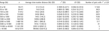
Table 1 shows the values for the two LD measures at various inter-marker distances. At an average distance of 31 kb, r 2 and |Dʹ| were 0.18 and 0.50, respectively, and the majority of the marker pairs (17 324 out of 18 271) displayed r 2⩾0.20. Both measures rapidly decayed by distance with more marked degradation rates for the r 2 measure. As a result, markers spaced 75 kb apart had r 2 and |Dʹ| values equal to 0.09 and 0.35, respectively. At the other extreme, markers spaced >40 Mb showed average values of r 2 and |Dʹ| equal to 0.004 and 0.085, respectively. Table 2 displays the values for the two LD measures at various distances for syntenic adjacent markers. Here, r 2 and |Dʹ| values for markers spaced up to 50 kb apart were 0.182 and 0.52, respectively, whereas markers spaced 50 to 100 kb had corresponding values of 0.10 and 0.37, respectively. Figure 1 displays a plot of the observed rʹ2 using pooled data (all autosomes). In contrast to the Frizarta breed, both LD measures were remarkably high in the EF breed with LD persisting over thousands of base pairs (Table 3).
Linkage disequilibrium decay by distance (⩽1500 kb) using pooled estimates of
 $$\hat{r}^{2} $$

Linkage disequilibrium measures at various inter-marker distances (n: number of marker pairs)

Linkage disequilibrium measures at various inter-marker distances of syntenic adjacent markers (n: number of marker pairs)

Linkage disequilibrium measures at various inter-marker distances of syntenic adjacent markers (n: number of marker pairs) in East Friesian sheep (brown and white) (total n=48, white: 9) (n=24 216)

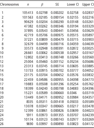
Table 4 displays LD decay rates (β) along with 95% confidence intervals (CI) across the 26 autosomes. Linkage disequilibrium decay rates varied considerably across the 26 autosomes, with lowest rates estimated for Oar2 and Oar1 (β=0.02185 and β=0.02798, respectively) and highest rates for Oar6 (β=0.05706), Oar12 (β=0.0546), Οar17 (β=0.05508) and Oar21 (β=0.05311). Using pooled data from all markers across the 26 autosomes, the average value for β was as high as 0.03391 (95% CI: 0.03372 to 0.0341). The weighted (by the number of markers per chromosome) β was equal to 0.03547.
Estimates of linkage disequilibrium decay by distance (β) with SE by chromosome (lower and upper 95% confidence interval (CI) are also shown (n: number of pairs of markers per chromosome)

Estimation of Ne
Table 5 and Supplementary Figure S1 present the estimated N e at three past time points. Based on the r 2 values for the 3000 kb fragments across the 26 autosomes, the estimated N e ~14 generations ago (year 1963) ranged from 458 to 739 individuals. The average N e was 578 individuals whereas the weighted (by the number of the r 2 estimates per chromosome) was 549 individuals. Using the 4500 kb fragments, the estimated N e ranged from 398 to 625 individuals, 9.3 generations ago (year 1981). The average N e was 492 individuals, whereas the weighted (by the number of r 2 estimates per chromosome) was 463 individuals. Finally, the estimated N e , based on r 2 values of the 40 000 kb fragments, one generation ago (year 2012), ranged from 165 to 237 individuals. The average N e was 196, whereas the weighted N e (by the number of r 2 estimates per chromosome) was 187 individuals.
Estimation of effective population size of the Frizarta sheep breed and migration rate at three past time points (years)

1 c estimated from function: t=1/(2c).
2 1000 kb≈0.012M.
3
Effective population size,
 $$N_{{e(t)}} {\equals}{{1{\minus}\hat{r}^{2} '} \over {4c\hat{r}^{2} '}}$$
.
4 Weighted estimate.
Population structure and genetic differentiation
Supplementary Figure S2 shows a two-dimensional plot of the MDS analysis. This plot suggests that the samples come from a genetically homogenous population, forming a circle, with no apparent clusters. Note that discrimination of animals between herds is apparent only when herds are known (denoted with different colors). In contrast to MDS analysis, the heat map of the GRM (Supplementary Figure S3) has revealed a clear population structure at the herd level. Note, however, that k-means clustering (with k=2 to 8) did not assign animals to herds according to their genomic relationships and only the EF cohort forms a distinct cluster (Supplementary Figure S3). Table 6 shows the pair-wise F ST values of the seven herds. Generally, F ST values were relatively low ranging from 0.02484 (herds EL01311762 to EL01315078) to 0.06761 (herds EL01308638 to EL01315608). The average F ST was 0.03859 (SD=0.027013). Such relatively low F ST values indicate that the seven herds are either sharing their genetic material through high levels of inter-breeding or they originate from populations that experienced the same or comparable levels of admixture events. Supplementary Figure S4 is a graphical representation of the F ST distances as depicted in a two-dimensional plot from the MDS analysis. Note the relative proximity of herds ΕL01301910 to EL01315608 in contrast to the remoteness of herds EL01315608 to EL01308638. Furthermore, the plot of the F ST values by herds’ geographical distances (Supplementary Figure S4) suggests that there is no gene flow between herds as F ST values were independent from herds’ distance.
Pair-wise F ST values of Frizarta sheep herds with 95% confidence interval (CI) (number in brackets denote sample size)

Estimation of migration rate (m)
Table 5 shows the estimated migration rates (m) at three past time points: at the onset of the breed formation (year 1963), at the end of admixture/migration events (year 1981) and one generation ago (year 2012). Based on the formula of (Nei and Chakravarti, Reference Nei and Chakravarti1977), F
ST
was as high as 0.00091, 0.00498 and 0.03377 at the three time points, respectively. Note that the most recent F
ST
estimate (based on the weighted N
e
) is 0.03377 and is clearly lower than the genomic data estimate (F
ST
=0.03859). If we, however, account for sampling size (S) and the Allendorf–Phelps effect (Allendorf and Phelps, Reference Al-Mamun, Clark, Kwan and Gondro1981), then the expected value of F
ST
is given by the equation
 $$E\left( {\hat{F}_{{ST}} } \right)\,\approx\,F{}_{{ST}}{\plus}{1 \over {2S}}{\plus}{1 \over {2N{}_{b}}}$$
(Waples, 1998) where S is the sample size and N
b
the number of effective breeders. For S=503 and assuming N
b
=187.4, the expected value of F
ST
is 0.03736 which is in closer agreement to the genomic data estimate (0.03859). This value of F
ST
implies that only 4% of the total genetic variability in the whole population can be attributed to the differences among herds. Furthermore, at the beginning of the admixture events, the m rate was as high as 0.50 (year 1963). This means that on average 0.50 of the individuals in the herds were immigrants implying the use of only EF rams for breeding. Lower m rates were estimated at the end of the admixture events (m=0.108, year 1981), whereas some migration rate could also be detected at the most recent years (m=0.038, year 2012). This result may not be surprising even for completely isolated populations that were connected or had experienced similar admixture events in the past.
Genomic inbreeding coefficients
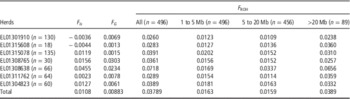
Table 7 presents the three genomic inbreeding coefficients per herd and overall. Negative F IS values were estimated for herds EL01301910 and EL01315608 whereas the highest value (0.0455) was estimated for herd EL01308638. With regard to F G , estimates were highest for herds EL01308765 (0.0303) and EL01308638 (0.0234). Using all ROH lengths resulted in highest F ROH estimates for herd EL01308638 (0.0718). Notably, in all herds, the highest inbreeding coefficients were estimated using ROH lengths >25 Mb implying most recent parental relatedness of animals. Furthermore, the pair-wise Spearman correlations between the genomic inbreeding coefficients were: F IS −F G =0.68, F IS −F ROH=0.82 and F G −F ROH=0.21. Note that, from the three pair-wise correlations, the highest correlation was attained between the F IS and F ROH coefficients.
Estimates of inbreeding coefficients per herd and overall

ROH=runs of homozygosity.
Discussion
Population structure and genetic differentiation
Various approaches were employed here to detect population structure and genetic differentiation of herds. Multidimensional scaling analysis and k-means clustering suggested a relatively genetically homogenous population, F ST values indicated relatively little genetic differentiation of herds and finally the heat map of the animals’ genomic relationships showed that the seven herds represent different genetic entities. Furthermore, given that there is no apparent relationship between the F ST values and the herds’ geographical distribution, herds can be viewed as closed populations with no apparent gene flow between them. All historical reports as well as personal communication with elderly farm owners support the scenario that this synthetic population resulted from admixture events, in the 1960s. What might have been the exact mode of admixture for this population? There are two possible, although extreme, scenarios here. In the first, the hybrid population was created by a single event of intermixture, in a single generation. This model is referred to as the intermixture or the hybrid isolation (HI) model (Long, Reference Long1991; Pfaff et al., Reference Pfaff, Parra, Bonilla, Hiester, McKeigue, Kamboh, Hutchinson, Ferrell, Boerwinkle and Shriver2001). In the second model, admixture occurred at a steady rate in every generation through diffusion from the donor population, that is EF into the recipient local population. This process is referred to as (continuous) gene flow (CGF) (Long, Reference Long1991; Pfaff et al., Reference Pfaff, Parra, Bonilla, Hiester, McKeigue, Kamboh, Hutchinson, Ferrell, Boerwinkle and Shriver2001). Whatever the mode of admixture, it is expected to have an impact on the LD pattern observed in the population. We discuss this issue in more detail in the next section.
Linkage disequilibrium levels and linkage disequilibrium decay
In a crossbred population, LD is composed of two parts. The first part is the average LD that existed within the parental populations (old LD), and the second part is LD generated in the cross as a result of differences in gene frequencies between the parental breeds (new LD), whereas the old LD is confined to shorter distances due to the accumulation of recombination events, the new LD extends over longer intervals (Toosi et al., 2010) but breaks down rapidly with random mating (Pritchard et al., Reference Pritchard, Stephens, Rosenberg and Donnelly2000). Pfaff et al. (Reference Pfaff, Parra, Bonilla, Hiester, McKeigue, Kamboh, Hutchinson, Ferrell, Boerwinkle and Shriver2001) have shown, via computer simulations, that the CGF model results in a retention of LD over relatively large (>10 cM) chromosomal segments. However, this is not the case in the HI model where a rapid decay of LD by distance is observed. In the present study, LD declined significantly over just a few thousand base pairs at a remarkably rapid rate conforming to the HI model. Such LD decay rates are usually observed in crossbred chicken (Fu et al., Reference Fu, Dekkers, Lee and Abasht2015) and cattle populations (Lu et al., Reference Lu, Sargolzaei, Kelly, Li, Vander Voort, Wang, Plastow, Moore and Miller2012) when contrasted to purebred breeds. However, the mating system alone does not always predict the structure of LD as other factors like the sample under analysis or the mating history can affect the LD pattern as well.
The LD levels observed in the population can be used to predict the power of GWAS based on the density of the marker set employed. In the literature, three different threshold levels for r 2 have been proposed: 0.2 (Meuwissen et al., Reference Meuwissen, Hayes and Goddard2001), 0.25 (Qanbari et al., Reference Qanbari, Pimentel, Tetens, Thaller, Lichtner, Sharifi and Simianer2010) and 0.33 (Ardlie et al., Reference Ardlie, Kruglyak and Seielstad2002). In the present study, values of r 2 close to 0.20 were attained for markers spaced 30 kb. This means that the 50k SNP panel with an average inter-marker distance of 50.9 kb is not sufficient to capture the LD information required for GWAS. In order to cover a total length of 2.61 Gb (size of the ovine genome), the number of SNPs required would be 87 000 (2.61 Gb/30 kb). Assuming that about 20% of the SNPs do not meet the QC criteria, the number of SNPs that should initially be available, rises up to 110 000. These figures are valid when the threshold value of r 2 was set to 0.20. When higher r 2 between markers (e.g. 0.33) is desirable, then even a denser marker panel should be used. Given that, the high-density chip with 600 k SNPs (Kijas et al., Reference Kijas, Lenstra, Hayes, Boitard, Neto, Cristobal, Servin, McCulloch, Whan, Gietzen, Paiva, Barendse, Ciani, Raadsma, McEwan and Dalrymple2014) is a very useful tool for performing more efficient and accurate GWAS in the breed.
In sheep, there are a number of studies reporting LD estimates obtained in purebred populations. In the French Lacaune dairy sheep, r 2 values of 0.13 for an average distance between SNPs of <50 kb are reported (Baloche et al., Reference Baloche, Legarra, Sallé, Larroque, Astruc, Robert-Granié and Barillet2014). In the Spanish Churra dairy sheep, r 2 values as high as 0.33 for SNPs up to 10 kb apart and 0.061 for SNPs separated by 200 to 500 kb are reported, whereas SNPs separated by >50 Mb showed an average r 2 equal to 0.003 (García-Gámez et al., Reference García-Gámez, Sahana, Gutiérrez-Gil and Arranz2012). Using 51 446 SNPs, in a sample of Sarda rams, Usai et al. (2010) estimated an average r 2 value of 0.072 over 1000 kb. Mastrangelo et al. (Reference Mastrangelo, Di Gerlando, Tolone, Tortorici, Sardina and Portolano2014) reported average r 2 values for all pairwise combinations of SNPs pooled over all autosomes as high as 0.058±0.023 for Valle del Belice, 0.056±0.021 for Comisana and 0.037±0.017 for Pinzirita breeds. Most recently, Mucha et al. (Reference Mucha, Bunger and Conington2015) reported an average r 2 of 0.20 for markers spaced 50 kb apart in a population of the Texel sheep. In that study, LD declined from 0.15 to 0.07 and to 0.04 at inter-marker distances of 100, 1000 and 2000 kb, respectively. It should, however, be noted that comparison of LD levels across different studies is not straightforward, because of several factors such as sample size, type of LD measures (Dʹ or r 2), marker types (microsatellite or SNP), marker density and distribution as well as population history and demography (Qanbari et al., Reference Qanbari, Pimentel, Tetens, Thaller, Lichtner, Sharifi and Simianer2010).
Apart from the inter-marker distance, LD levels are also dependent on the MAF threshold with higher MAF thresholds resulting in higher LD levels, especially for short distances (Reich et al., Reference Reich, Cargili, Boik, Ireland, Sabeti, Richter, Lavery, Kouyoumjian, Farhadian, Ward and Lander2001, Qanbari et al., Reference Qanbari, Pimentel, Tetens, Thaller, Lichtner, Sharifi and Simianer2010). In cattle, Khatkar et al. (Reference Khatkar, Nicholas, Collins, Zenger, Cavanagh, Barris, Schnabel, Taylor and Raadsma2008) have shown that MAF affect r 2 but not Dʹ values for closely located markers (<40 kb). To ensure a more accurate estimation of LD levels, a relatively high level of MAF was used in the present study (MAF>0.20). Linkage disequilibrium levels estimated here were higher than those estimated by applying a lower MAF threshold (MAF>0.05) (Kominakis et al., Reference Kominakis, Hager-Theodorides, Zoidis, Saridaki, Antonakos and Tsiamis2015). In the present study, the use of a higher MAF has also resulted in a significant reduction of the number of SNPs available for further analysis.
This is the first study reporting LD decay rates per chromosome in sheep, using SNP data. To our knowledge there is only one study reporting β estimates in sheep and this was based on microsatellite markers (Meadows et al., Reference Meadows, Chan and Kijas2008). The behavior of LD, measured by the coefficient β was found to differ markedly between the 26 autosomes. Linkage disequilibrium decayed fastest within the short chromosomes (e.g. chromosome 12) whereas LD decayed slowest within the long chromosomes (e.g. chromosome 1). The β coefficient represents a combination of local recombination rate and local N e . Assuming that N e does not vary across chromosomal regions due to selection, then β may be interpreted as a measure of recombination rate. Low β values imply low recombination rates and vice versa. In humans, a strong correlation between recombination rate and chromosome size is well documented with smaller chromosomes having higher recombination rates than larger chromosomes (Petes, Reference Petes2001, Sun et al., 2005). Studies on other livestock species such as the pig, have shown a differential pattern of LD decay across the chromosomes with highest recombination rates for chromosomes 10 and 12 and lowest for chromosomes 1 and 13 (Muñoz et al., Reference Muñoz, Alves, Ramayo-Caldas, Casellas, Rodríguez, Folch, Siliõ and Fernández2012, Wang et al., 2013).
The application of F ST to estimate N e m (or m as in here) has attracted considerable criticism (e.g. Whitlock and McCauley (1999) and references therein) for its underlying assumptions, including that populations have the same and constant sizes, exchange equal numbers of migrants and that have approached equilibrium between gene flow and genetic drift. Furthermore, the ‘Continent-Island’ and the ‘island model’ were interchangeably used here. Obviously, such conditions do not apply to our population. Despite the fact that there are more powerful approaches to estimate m and that F ST may offer biased estimates, it still remains a useful measure of average effects of migration on gene flow (Neigel, Reference Neigel2002). In our case, such a ‘simplistic’ approach yielded m estimates that seem to comply with the history of the population.
Effective population size
Finally, we used genomic data to make inferences about N e at three past time points. At the most recent time, the inferred N e was of moderate size, around 190. This figure is significantly smaller than those reported by the SheepHapMap project (Merinos=853, Poll Dorset=318, Border Leicester=242; Kijas et al., Reference Kijas, Porto-Neto, Dominik, Reverter, Bunch, McCulloch, Hayes, Brauning and McEwan2012). Most of the sheep breeds analyzed in the SheepHapMap project had large N e , that is 600 for Spanish Churra and 795 for the Finnsheep breed. In a study on five populations of Australian domestic sheep, Al-Mamun et al. (Reference Allendorf and Phelps2015) reported N e estimates of 140 for Border Leicester, 152 for Poll Dorset and 348 for Merinos. For the Spanish Churra dairy sheep relatively low N e =128 has also been reported (García-Gámez et al., Reference García-Gámez, Sahana, Gutiérrez-Gil and Arranz2012). Beynon et al. (Reference Bjelland, Weigel, Vukasinovic and Nkrumah2015) reported estimates of N e ranging from 88 (Kerry Hill) to 825 (Badger Faced) for 18 Welsh sheep breeds with an average estimate of N e =316.
Using the Wright’s equation (1931) N e =(4N m N f )/(N m +N f ) with N f =1750 ewes (census ewes population) and N m =87 rams (assuming a sex ratio 1 : 20) then N e =333, a figure that is clearly higher than the genomic data based estimate. Apparently, the use of the Wright’s equation is a rough approximation that does not take into account, inbreeding, genetic drift and selective breeding. Leroy et al. (Reference Leroy, Mary-Huard, Verrier, Danvy, Charvolin and Danchin-Burge2013) reported an average N e of 189 (range 28 to 249) for 40 sheep breeds based on genealogical methods and more specifically on the individual co-ancestry rate. The respective estimate when the individual inbreeding rate was considered was 191 (range: 38 to 675). Using the sex ratio equation always resulted in inflated N e estimates for 140 breeds in four species, sheep included (Leroy et al., Reference Leroy, Mary-Huard, Verrier, Danvy, Charvolin and Danchin-Burge2013). It should, however, be noted that N e estimates may also vary across studies as the result of application of different estimation methods.
Inferred N e declined progressively from 578 to 492 within a period of about four generations, whereas a more rapid decline (from 492 to 192) was observed during the latest generations (generations 5 to 13). This decline may be attributed to various reasons such as high selection pressure, low genetic diversity and inbreeding. The relatively high estimates of inbreeding coefficients based on ROH measuring >25 Mb suggest that recent inbreeding might have been a significant determinant of the current N e. Apart from inbreeding, an admixture event may also have effects on the inferred N e , with higher estimates for the generation in which the admixture event is occurring (Kijas et al., Reference Kijas, Porto-Neto, Dominik, Reverter, Bunch, McCulloch, Hayes, Brauning and McEwan2012). However, this finding clearly does not apply in our case as the effects of admixture on estimates of N e are expected to be minimal for generations that are not within 100 generations of the admixture event (Kijas et al., Reference Kijas, Porto-Neto, Dominik, Reverter, Bunch, McCulloch, Hayes, Brauning and McEwan2012).
In the present study, a closer relationship between the F IS and F ROH coefficients and poor correlations between F G and F ROH were observed. Zhang et al. (2015) have also found highest correlations between F IS and F ROH computed from either 50k or sequencing data, in three dairy cow breeds. Poor correlations between F G and F ROH have also been reported by Zhang et al. (2015) and Mastrangelo et al. (Reference Mastrangelo, Tolone, Di Gerlando, Fontanesi, Sardina and Portolano2016). Current results suggest that the use of dense genetic marker information is also valuable for depicting the existing inbreeding levels allowing for a more efficient control of the rate of inbreeding increase in the population.
In conclusion, samples of the Frizarta breed used here suggest a relatively homogenous population of moderate effective population size that was formed by single intermixture events during the 1960s. Genome wide association studies are expected to greatly benefit in accuracy and power when a denser than the 50k SNP panel is employed.
Acknowledgments
This study was supported by the Action ‘Cooperation 2011’ of the Greek Ministry of Education and Religious Affairs (grant no. 447919/11SYN_3_1087). The authors thank the two anonymous reviewers whose comments helped improve and clarify this manuscript.
Supplementary materials
To view supplementary material for this article, please visit https://doi.org/10.1017/S1751731117000428