Introduction
In developing countries, where agriculture is mainly rain-fed, production conditions follow changing rainfall patterns. In addition, levels of production may continually vary according to variations in prices and a range of other factors, some of which could be fairly rapid. The long-run effects of these changes may not be clearly understood. For example, an increase in the price of beef may have little effect on production in the short run because producers have committed their resources to that production. But in the long run they can change the amount of resources used to either increase or reduce their production, or switch to other types of production altogether. Thus, the long-run price elasticity of herd off-take, for example, would be expected to exceed the short-run elasticity. Implicit in this is some kind of dynamics of economic change, the reason for postulating a dynamic model in this paper.
Off-take is an important measure of herd dynamics and therefore a means for estimating output from a production unit, such as a ranch. Herd off-take is the percentage of the current year's herd that is removed for commercial and non-commercial reasons (Heath, Reference Heath, Prins, Grootenhuis and Dolan2000; Nyariki et al., Reference Nyariki, Makau, Ekaya and Gathuma2005). Although non-commercial transactions contribute significantly to the total herd off-take, especially in pastoral production systems, commercial off-take – livestock units that leave the herd for cash sales – constitutes the main form of off-take, especially from ranching.
The livestock sector in Kenya, which comprises pastoral systems, smallholder production, and ranching, contributes about 50 per cent of the country's agricultural gross domestic product (GDP). The sector accounts for 90 per cent of employment and more than 95 per cent of household incomes in the arid and semi-arid lands (ASALs), which form about 80 per cent of the country's land area. Ranching, which denotes extensive livestock husbandry on natural or improved pasture, is undertaken in the rangelands and contributes about 36 per cent of the national meat output in Kenya (Nyariki et al., Reference Nyariki, Makau, Ekaya and Gathuma2005).
Livestock from ranches are sold on-farm or in the local markets, and also often shipped abroad, mainly to Saudi Arabia. These markets attract different prices for the rancher. The mid-1980s marked the beginning of crucial policy changes in Kenya, with the implementation of price decontrols and market liberalization. As a result, ranchers started enjoying higher prices. Beef producer price control policy was waived in 1987, and the prices of animal feeds and the dairy industry were liberalized in 1989 and 1992 respectively. Immediately after liberalization, beef prices rose rapidly, indicating that the price ceilings imposed by the government were below the equilibrium price generated by demand and supply. The rise in prices was also driven by high human population growth, at more than 3 per cent a year, and increasing per capita GDP on average (ROK, 2004a).
Commercial off-takes from ranches have implications on incomes, food security, poverty alleviation, and environmental health within ranches and in the country as a whole. To maintain the food security status and living standards of the populations that depend upon ranch off-takes, if ranching in the rangelands is not economically and environmentally sustainable, would require government allocating a significant portion of the national budget to either develop policies that would help the industry to be sustainable or secure alternative livelihoods for the affected populations; a budget that would otherwise support other areas of development such as road infrastructure, education, and security. If the off-takes do not provide adequately for the ranch operators, the operators and their families may be forced to look for alternative sources of livelihood. They may resort to other means of exploiting the rangelands, including charcoal burning, cultivation, and many forms of ‘natural resource mining’, which are unsustainable and would cause environmental degradation. If off-take rates were curtailed because of inadequate markets, this would lead to excessive accumulation of livestock on the rangelands, in turn causing over-use and degradation of the natural environment, and eventual loss of livestock and livelihoods.
It is hypothesized that ranchers in developing countries, just like their counterparts in developed countries, seek to maximize their income over time by selling or purchasing stock, by breeding or slaughtering stock and a wide range of other activities, and hence are responsive to change in price and other production conditions. Even though income or profit maximization may not be the only objective, it is considered to be an accurate predictor of producer behaviour. A majority of ranchers are, therefore, thought to face this complex problem of income maximization, for the most part by repeating what they usually do or by changing this action in the light of new weather or price conditions, or expectations based on their experiences. Understanding the factors that play a major role in influencing ranchers' economic actions over time may be one of the initial, but significant, steps towards contributing to efforts of improving production, incomes and the associated natural environment in this sector in developing agriculture.
The paper discusses reasons why variables were selected and how they were measured, and why the dynamic model was adopted. In this way, one can appreciate and understand the economic situation underpinning the model of choice. Also, a discussion is provided regarding the suitability of the final model used with the pooled data so as to obtain efficient and consistent parameter estimates.
Area of study and data collection
The data for this study were collected from Laikipia District, situated on the equator in central Kenya. The district lies east of the Great Rift Valley and covers about 9,700 km2 (ROK, 2004b). In the west and south-west, the district is hilly and consists of upland forests at elevations above 1,900 m. As one moves down the slope from the west to the east and north-east, towards Isiolo District, so rainfall diminishes – from an annual average of 900 mm in the west to as little as 400 mm in the north-east – while temperature and evapo-transpiration rise. The district receives an annual average precipitation of about 700 mm. This gives a wide range of agro-ecological zones, from the hills where wheat is grown, to the lower plateau perhaps best suited to grazing livestock but where crops such as maize, beans and potatoes may be planted at the risk of frequent harvest failures. The rainfall regime is bimodal, long rains falling in May to August and short rains in September to December, giving two cropping seasons (Jaetzold and Schmidt, Reference Jaetzold and Schmidt1983). The district is one of those with the greatest concentration of commercial ranches in the country. Most ranch land, consisting of approximately 78 per cent of the district, is situated on the Laikipia plateau at an elevation of between 1,500 and 1,800 m, in Ecological Zones IV to VI (Heath, Reference Heath, Prins, Grootenhuis and Dolan2000). The vegetation here is dominated by grassland mainly made up of Themeda triandra and Pennisetum mezianum, Acacia bushland consisting mainly of Acacia drepanolobium and A. Seyal with T. triandra, and leafy bushland dominated by Euclea divinorum, Carissa edulis, Rhus natalensis, and Tarchonanthus camphoratus (Pratt and Gwynne, Reference Pratt and Gwynne1977).
Ten ranches out of 60 operating in the study area were selected through simple random sampling. A questionnaire was used to collect primary data from this sample. Secondary data on herd sizes, animal numbers sold, prices received, costs incurred, incomes accrued, rainfall, and other variables for the ten ranches were obtained from ranch records. Adequate secondary data covering a period of 17 years (1986–2002) were provided by the selected cross-section of ranches. These data were pooled to produce a panel of 170 sample points. Variables related to beef cattle production were obtained by using comparative data based on animal units. These data enabled the apportionment of variables such as incomes, costs, land area, and stocking rates between beef animals and other enterprises.
Selection and measurement of variables
In formulating the model, the extra variables (other than price) were selected a priori and tested singly to determine which would have an influence on off-take. These factors were then included in the final model. A preliminary correlation analysis of the variables was carried out, and an appropriate choice was made between those variables that were found to be highly correlated. The variables used in the final regression are off-take, price, climate, stocking rate, and a shift dummy.
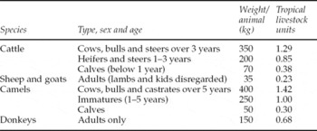
There are various forms of livestock-related off-take. These include live animals, milk, meat, hides, skins, and manure. Off-take may thus be seen as removal of live animals or their products from the herd for consumption within the ranch or for outside destinations such as the market. The most important of the livestock-related off-take is in the live form. Livestock off-take can thus be generally defined as the percentage of the current year's herd that is removed through sales, deaths, gifts, home-slaughter, or even theft (Nyariki et al., Reference Nyariki, Makau, Ekaya and Gathuma2005). This kind of off-take is calculated from the total herd size kept in a year (Nyariki and Munei, Reference Nyariki and Munei1993). However, commercial off-take constitutes the percentage of livestock units that leave the herd for cash sales each year. Livestock units (LUs) are standardized animal units to which different ages, types, or species of livestock are related for purposes of matching forage availability to animal requirements (Pratt and Gwynne, Reference Pratt and Gwynne1977; Gittinger, Reference Gittinger1982; Evangelou, Reference Evangelou1984; Nyariki and Munei, Reference Nyariki and Munei1993; Upton, Reference Upton1993). Usually the unit is taken to be either a 450 kg live weight steer, with a daily dry matter requirement of 10 kg, or a mature zebu with calf at foot weighing 250 kg, with a dry matter requirement of 6.5–8.5 kg. This latter measure is also referred to as tropical livestock unit (TLU) (Grandin and Bekure, Reference Grandin and Bekure1982) and was adopted in this study. The relationship between other livestock and the standard unit is usually based on relative live weight, where livestock weights cannot be measured directly in the field (Sullivan et al., Reference Sullivan, Farris and Simpson1982). On this basis, about 7 sheep or goats are taken as roughly equivalent to one TLU (Dahl and Hjort, Reference Dahl and Hjort1976; Gittinger, Reference Gittinger1982). More appropriately, however, LUs are based on feed consumption requirements, with an adult zebu milking cow treated as the standard and given a value of unity (Upton, Reference Upton1993; Nyariki et al., Reference Nyariki, Makau, Ekaya and Gathuma2005) (see table 1 for details). Off-take was mainly from cattle herds, as sheep and goats formed an insignificant proportion (less than 2 per cent) of the total LUs in each ranch. After determining ‘output’, the off-take of the herd – with the total herd size being taken as ‘input’ – was estimated. In a steady state production system, off-take rates measured this way would roughly measure herd productivity (Baptist, Reference Baptist1988; Upton, Reference Upton1993) – a general term frequently associated with ratios of output to input and sometimes with ratios among outputs and inputs (Edwards, Reference Edwards1985).
Livestock conversion rates

Source: Nyariki et al. (Reference Nyariki, Makau, Ekaya and Gathuma2005).
Price plays an important role in any production system. In a relatively free market economy such as Kenya's, it is assumed that ranchers are rational so that when prices offered are high, they will endeavour to increase stock for sale. It is, however, expected that the higher the price at any unit-time period, or the greater the current rate of price change, the greater the desired future herd. This may cause a reduction in off-take in the immediate future. As argued by Jarvis (Reference Jarvis1974) and Ndzinge et al. (Reference Ndzinge, Marsh and Greer1984), an increase in the price of beef, which is not expected to last, could lead to increased rather than decreased slaughter only in the short run. In the not-very-short run, however, slaughter may be negative because animals are withheld to permit increases in future output. The traditional Nerlove supply model is essentially a relationship between price and a response factor. However, the economic reality that ranchers face is more complex than this. Hence, Nerlove's conventional and rather simplistic model was extended to include extra explanatory variables. In order to avoid a spurious regression between price and off-take, the annual beef prices offered to ranchers were deflated using an average consumer price index to derive real prices. However, to confirm the stationarity of the deflated prices, the unit root test was carried out.
Perhaps the single most important factor in most types of agricultural production is rainfall. This is more so in developing countries where agriculture is largely rain-fed. Higher rainfall leads to more and better pastures, thereby increasing off-take. However, higher total amounts of rain per se may not translate into greater output, especially in the ASALs where rainfall may only be received for a short period. The distribution of rain is important in influencing off-take. Therefore, in this analysis, distribution of rainfall, represented by the number of days of rainfall per year, was included, but not directly because it had shown a strong correlation with total rainfall. The inclusion was done by obtaining the average amount of rainfall by dividing total rainfall by the number of days it was received – to derive the variable herein referred to as climate.
The number of livestock units grazed on an area of land for a given period of time is the stocking rate, and affects the intensity of use of available resources, including forage. If extra animals are added to an already optimal stocking rate, the added animals will adversely affect the performance of other animals, causing output to drop. Average age at maturation will also increase. If a rancher is aware of the optimal carrying capacity of his ranch, he may not wish to hold more livestock than the land can sustain.
Preliminary analysis of the data showed that in some years there were dramatic increases in off-take while in other years there were large reductions in this variable. Close examination revealed that in the years when there were large upswings there was drought (rainfall of less than 300 mm/year), while in the years of downswings, rains were particularly good. These swings necessitated the use of a shift dummy in an attempt to take care of the dramatic changes in off-take, thus


where D is the dummy and t is the year of observation.
Model specifications
There are many ways through which a rancher could effect changes in off-take rates, but there are also many factors over which the rancher has little or no control. The prime examples are item costs and market values. Changes in the cost of inputs or climatic conditions or in the value of products during the production period can affect the economic decisions of a rancher, resulting in changes in off-take rates. Therefore, ranchers make their production decisions under uncertainty (Nyariki and Wiggins, Reference Nyariki and Wiggins1999). Furthermore, animal output is subject to a number of biological factors which are beyond the rancher's control and may cause large and random fluctuations in herd off-take. Hence, the perception of what is the optimum off-take rate, from the point of view of the rancher, is expected to continually change. Faced with changing production conditions and the fact that change in production cannot be instantaneous, it takes time for ranchers to achieve the desired level of off-take. They may also have to take production decisions based on expected prices and other variables. All the rancher's economic judgements are, therefore, expected to consider the present price structure and other factors, and the extent of change that is likely (Nyariki and Munei, Reference Nyariki and Munei1993). In these circumstances, off-take response analysis cannot be meaningfully undertaken within the framework of a static model.
The following general equation, which is a DL model, represents the base dynamic model adopted
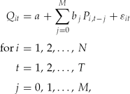
where N is sample size, T the length of time-series in years, and M the total number of lags in years.
From this equation, three main specifications of a dynamic model obtain. These are the Koyck distributed lag model, adaptive expectations (AE) model and partial adjustment (PA) model. Because of the correlation between lag variables, the DL model suffers serious multicollinearity and therefore cannot be estimated in this form. The solution is to assume that the impact of the explanatory variable declines geometrically and the coefficients are all of the same sign so as to obtain finite lags. However, in this model, first proposed by Koyck, the usual OLS estimation is still inappropriate as it would lead to biased and even inconsistent estimators, thereby yielding misleading results, because of the introduction of a lagged dependent variable (Qt −1), which is bound to be correlated with ɛt via the presence of ɛt −1 (Gujarati, Reference Gujarati1988).
The AE model is an expectations formulation model, developed by Nerlove in 1958, in which producers are thought to be changing production according to their revision of what they perceive as normal based on various occurrences. Nerlove's model, therefore, reflects dynamism in the specification, which is a realistic situation since stationary states seldom occur in the real world. It is assumed in this model that the regressor takes on expected (optimal) values. For example, in the present case, it would be assumed that ranchers' efforts to increase off-take depend on what they perceive the general level of beef prices to be in the current period. This implies that ranchers may reduce off-take currently if they expect prices to be higher in the future. It is also assumed that expectations are a weighted average of present prices and expectations in the previous periods. The main problematic similarity between the Koyck and AE models, however, is that they both have a composite residual. Thus, the AE model also suffers the serial correlation problem, causing OLS estimates to be biased. In addition, the AE model is a crude representation of the real world because its estimation is conceptually based on past experiences, and is therefore not forward-looking.
The concept of the PA or stock adjustment model, also developed by Nerlove (Reference Nerlove1958), refers to a situation where because production of a certain good is slow to change, say, due to the amount of capital involved or biological reasons, the move towards a desired equilibrium level is not accomplished entirely within a unit period of time; only a partial adjustment of stock takes place, so the total shift towards equilibrium covers several periods.
Suppose that the desired level of off-take Qt is Q t*, which is assumed to be related to an exogenous variable Pt, the following model would apply

Because of adjustment difficulties ranchers cannot set Qt equal to Q t* in every period. Rather, Qt is assumed to adjust partially in the direction of Q t* according to the following equation

where 0 < g < 1.
Equation (1) shows that the desired level of beef production depends on the current prices, while equation (2) shows that actual shift in production in one period (Qt – Qt −1) is only a fraction g of the distance (Q*t − Q t−1) to be covered in order to get to the equilibrium level. Since Q* is not observed in the field, and only conceptually exists in the rancher's mind, a guess has to be made as to what factor might be influencing its level. The factor might be price, which then gives equation (1). But this could be wrong because Q* may (and does) depend on other variables as well. Such are some of the situations frequently faced, and it is necessary to rely on personal knowledge of the economic behaviour of the phenomenon being investigated.
In order to use observed data (Q and P) to estimate the coefficients in equations (1) and (2), Q* is substituted from (1) into (2) to obtain

Estimates of a, b, and g can now be obtained using the OLS process. Equation (3) is the same as the Koyck and AE models. The only difference among the three is that the residual term in (3) is not composite. If the residual term in (3) is serially uncorrelated, so will gɛt be. Also, since ɛt −1 is absent, no OLS bias will be caused even though Qt −1 is used as a regressor. However, the usual Durbin–Watson test will be inappropriate even in this case. Nevertheless, since the PA has fewer limitations, it seems to be theoretically and statistically tractable and was used for analysis in this paper. Furthermore, developments have been made on the Durbin–Watson test, which can be applied to autoregressive equations. Obviously, though, it does not imply that one can discriminate between models only on the basis of their convenience; economic judgement regarding the phenomenon being analysed must override.
It has been shown that the common feature of the three models, which possess a similar algebraic structure, is the presence of a lagged dependent variable (Qt −1) among regressors. This variable is used because past values of Q are a good guide, although not the real explanation of what determines it, to its current value.
From the foregoing, it can be observed that the shortcomings of the Koyck model include the unrealistic assumption that the dependent variable is affected by all past values of the independent variable(s), and the fact that the equation for estimation is rather complicated because of the composite residual, which invalidates the use of OLS estimation technique. The elimination of the Koyck model leaves the other two, which seem difficult to discriminate against because both types of lag are realistic and are likely to occur in ranching. Ideally, then, the two lags should be combined in a single model as Jennings and Young (Reference Jennings and Young1980) tried to do by generalizing Nerlove's supply model. However, as the two authors also acknowledge, the structure of the model and the error term become even more complicated, and the likelihood of the model being under-identified is greatly increased (Hebden, Reference Hebden1983). With these difficulties, therefore, one has to discriminate against one model. Fortunately, the PA model has two important advantages; it does not include a composite residual and the OLS estimation can be applied, unlike the AE model. Further, one does not have to assume, as in the AE model, that expectations adaptations are the same for each variable, which, apparently, is unreasonable.
The application of the most appropriate model is now explicitly shown through derivation of equations. Ignoring the i for the time being, for clarity reasons, the specific model can be expressed as follows


where:
Q*t = optimum off-take rate that ranchers would wish to attain (if there were no adjustment difficulties) at time t
Qt = actual off-take rate achieved at time t
Pt −1 = deflated price of beef per kg live weight lagged once
St −1 = stocking rate lagged once
Wt −1 = climate (total rainfall divided by number of days of rain) lagged once
Dt = dummy to capture the effect of drought at time t
λ = coefficient of adjustment
Except for drought, it was assumed that the rest of the explanatory variables would take at least one time-period to impact off-take; hence, they were lagged once. Equations (4) and (5) give the following equation to be estimated

The inclusion of variables S, W, and D was done after preliminary regressions against Q; using each variable singly showed that they might be important factors determining off-take. Demand for beef is assumed to be high and therefore ranchers would still secure markets for their increased supply. The corollary is that increased (or decreased) off-take does not change prices or any other exogenous factors in the short run as the proportion of supply from ranches compared to total beef supply in Kenya is small. So the situation in the short run should be that the variables are exerting effects on the response variable rather than the reverse; otherwise, there would be a breakdown of the assumptions made for the partial adjustment model.
Panel data model
The derived dynamic equation (6) was transformed to an appropriate panel data model. The data available were examined and their application carried out based on the structure of the model. Since sufficient time-series observations were unavailable for all the ranches, and since it would have been inappropriate to make generalized inferences on the response of ranchers from a single ranch, time-series data were pooled with cross-section data to form a panel. The assumption in pooling data is that cross-section parameters do not shift over time; otherwise, it would be inappropriate to do so. On the other hand, there might be time-series related explanatory variables such as lagged effects of prices, which could be included in a pooled model. Using panel data to include both time-series and cross-section variables then becomes theoretically useful (Pindyck and Rubinfeld, Reference Pindyck and Rubinfeld1998).
Several methods are available for analysing panel data. First, all cross-section and time-series data can be combined and an OLS regression is performed on the entire data set. Second, there is the covariance model, which involves the addition of dummy variables to the model to allow for the changing intercepts. Third, and the most popular of the procedures, is the error-components model, which has two specifications: the fixed effects model and the random effects model (Kim and Maddala, Reference Kim, Maddala, Baldev and Baltagi1992; Maddala, Reference Maddala2001). Lastly, there is the time-series auto-correlation technique, e.g. using the Cochrane–Orcutt procedure, which considers the fact that the error-term may be correlated over time and cross-section units (Thomas, Reference Thomas1993; Baltagi, Reference Baltagi2001). Except for the model adopted for analysis, the precise mathematical details of these procedures need not concern us.
All four mentioned estimation techniques give unbiased and consistent parameter estimates, and the main criterion for discrimination would, therefore, be that of efficiency. The error-components model is one of the most efficient because it is estimated using a form of GLS regression. However, the main problem with this technique is that OLS will not yield unbiased estimates when lagged dependent variables are included as regressors in the equation (see, for example, Davidson and Mackinnon, Reference Davidson and Mackinnon1993; Pindyck and Rubinfeld, Reference Pindyck and Rubinfeld1998), as is the case in the dynamic model adopted in this paper. Exactly how this arises is shown, for example, by Davidson and Mackinnon (Reference Davidson and Mackinnon1993), Robinson (Reference Robinson2003), and Wooldridge (Reference Wooldridge2003). Therefore, this leaves the time-series auto-correlation technique as the most appropriate in the present case, and it was adopted for analysis.
The Cochrane–Orcutt two-stage procedure
For exposition of the Cochrane–Orcutt procedure, consider a simple model

where

Each error structure is fixed to involve first-order serial correlation but ρ is allowed to vary from individual to individual unit. So the model is first-order autoregressive AR(1) in structure. With this model, efficient parameter estimates can be obtained by using a form of GLS process (Gujarati, Reference Gujarati1995). The Cochrane–Orcutt coefficients, ρi, are estimated from ρi* and are then used as a basis for the GLS regression. To estimate ρi* i = 1,2, . . ., N, OLS regression is carried out using the entire pooled sample after which the generalized difference of the original model is derived as shown in (8)


The Cochrane–Orcutt process in (8) validates the application of the OLS estimation to the general difference form of the pooled model. The final equation is obtained first by transforming the PA model in equation (6) to suit the data as follows: let

Equation (6) can now be written as

The generalized difference of equation (9) with the i introduced can then be written as

The variables and error term (marked θ) are differenced as shown in equation (8). After estimating equation (10), the values of a,b 1, . . ., b 4, λ are obtained by working backwards.
Before estimating equation (10), the unit root test of stationarity of the variables was carried out. All the variables were found to represent stationary time series at the 5 per cent level of significance. To illustrate with the deflated prices, the following equation was used

where ΔPt is the first-difference of the panel of prices, and the null hypothesis is set at δ = 0. If there was a unit root problem in the data, δ would be equal to zero. The results were as follows:
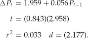
Since the results in equation (11) suggest that the error term is not autocorrelated – based on the Durbin–Watson (d) test – the stationarity of deflated prices can be proved by the Dickey–Fuller (DF) test, using the t-value (tau statistic). Since the computed tau value is 2.958, which is greater than the 5 per cent critical (DF) value of −2.895, the data did not exhibit random walk.
Results and discussion
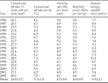
Before discussing the results of the regression analysis, it would perhaps be of interest to present some of the descriptive data of the analysis. Table 2 shows the average values of variables over the period of study. The data indicate that off-take rates ranged between 18 per cent (in 1986) and 29 per cent (in 2002). The low off-take rate of 1986 would have been mainly caused by the drought of the 1983/84 production year – a period in which some of the lowest stocking rates were registered. This situation is repeated immediately after the 1991/92 and 1995/96 periods of relative drought. While the low off-take rate in 1986 may have been influenced by weather, it is possible that the interplay of price and climate had the impact seen, the years having registered some of the lowest real prices. Producers obtained the lowest real producer prices in 1993 and 1994 – the years with some of the highest inflation rates in the 1990s decade. Since the inflation rate was among the lowest in 1986 (4.6 per cent) (ROK, 1980–2004), the low rate of off-take was more likely a result of drought, and therefore ranchers were rebuilding their stocks, which were reduced by the drought. Also, the scenarios in 1993/94 and 1998/99 were in large measure influenced by the drought of 1991/92 and the El Ñino of 1997/98. The former resulted in a glut of slaughtered stock, while the latter led to a withholding of stock due to favourable weather for stock expansion.
Sample means of variables over the period 1986–2002

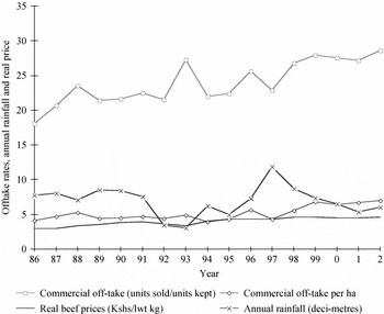
Table 2 shows that while there have been down-swings in off-take rates, the general trend has been upwards, albeit slowly. The plot in figure 1 clearly shows that off-take trend closely follows real price trend. It can also be noticed that stocking rates have been increasing in line with increasing prices; there has been less and less land allocated to a stock unit, an indication that stock has generally increased since the mid-1980s. Further, there was a marked increase in stock per unit land area and off-take between 1990 and 2002. In this period, real prices rose steadily. The rise in prices and the accompanying improvement in both stocking and off-take rates occurred after the liberation of the beef market in 1987 when producer and consumer prices were decontrolled, and at the beginning of the 1990s when a total waiver of controls in the beef and dairy industry in the country took place (ROK, 1996).
Trends in off-take rates, stocking rate and beef prices, 1986–2002

Figure 1 may be used to show how rainfall has been one of the contributing factors to changes in off-take since the mid-1980s. The two variables generally moved together for most of the study period. However, from the early 1990s, off-take continued to increase with real prices in spite of the rains, indicating that prices and other socioeconomic factors rather than climatic factors triggered this increase.
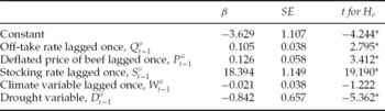
The estimates of equation (10) are presented in table 3. As shown by the corresponding t-values, four out of the five explanatory variables are significant. The adjusted R 2 value is high and indicates that 75 per cent of the total variation is explained by the variables. The F-statistic is significant (P < 5%) and therefore indicates that the variables as a group have a significant influence on off-take. The absence of auto-correlation in an AR model is proved by deriving h-values. The h-value of −1.209 (table 3) implies that auto-correlation is not a serious problem (Johnston, Reference Johnston1984; Thomas, Reference Thomas1993).
Estimated coefficients of equation (10)

Notes: *Significant at 5%; F = 128.532*, P < 5%, R 2 = 0.775, Adj. R 2 = 0.746, h = −1.209.
Working backwards using the results in table 3, equation (4) – the long-run equation of our interest – is given as

Lagged price (Pt −1) has a positive and statistically significant effect on off-take (table 3) implying that increasing prices lead to increased off-take rates in the immediate future. However, this does not necessarily imply that the response would be the same if there were longer price lags. It has in fact been shown in some studies, such as those by Jarvis (Reference Jarvis1974), Nyariki and Munei (Reference Nyariki and Munei1993), and Mugarura (Reference Mugarura2001), that cattle slaughter may (and would actually be expected to) show a negative response to certain price lags since animal output can be increased mainly by increasing the breeding stock, and ranchers would hold on to their animals for higher output. They may also withhold the animals from the market for further fattening to increase output per unit animal. Further, this response may occur in the simplest form of traditional pastoralism – which is non-market oriented. In this form of livestock rearing, pastoralists are thought to have a target cash income and when offered a higher price for their product, they can attain this level with a reduced supply. They would therefore have a perverse response to any changes that would increase their income beyond the target. However, there is never reason to expect commercial ranchers to reduce off-take when they attain a certain level of income. A negative response of a product to increased producer price is, nevertheless, rarely observed in agriculture as this behaviour contrasts with the supply response of most agricultural products.
The positive response of off-take to first-order price lags can be explained by the understanding that the decision to increase or reduce marketed stock in the event of a price change is made on the basis of expected prices, arrived at by considering past prices. Hence, ranchers would consider a ratio of their herd that they wish to put on the market based on the previous year's price. If a high price is expected to last – a judgement that would be arrived at after considering a series of past prices – a negative response of off-take would be the likely outcome. Thus, the immediate response is to increase stock to capture the benefits of increased price, or reduce stock to avoid loss of revenue in the event of reduced price. This is confirmed by the positive relationship between current off-take (Qt) and lagged off-take (Qt −1). In this respect, the theories of ‘partial adjustment’ and ‘adaptive expectations’ seem to converge.
The response of off-take in some years would, of course, be due to factors other than price, such as climate. Climate has a negative effect on off-take, though insignificant (table 3). The insignificance of this variable is most likely due to the inclusion of a shift dummy, which has a negative and significant coefficient and should explain how climate impacts ranchers' decisions. When drought occurs (t = 0 in Dt), ranchers tend to reduce their herd size to minimize losses caused by increased deaths. This leads to a glut of slaughtered stock in the market and, consequently, prices plummet. In the aftermath of a drought, herd sizes decrease due to the lagged effect of drought, leading to low off-take rates. Since supply is reduced, demand becomes relatively high and prices rise.
The frequency and severity of drought (Dt) influence range condition and trend, and the negative and significant response of off-take to the dummy is confirmation that livestock production in developing countries like Kenya mainly depends on climatic conditions. The negative effect is not surprising because ranchers can sustain herds from one production period to another in years of high rainfall to fatten them further, so that many animals that would have otherwise been disposed of are kept back. Consequently, off-take rates are kept low. On the other hand, ranchers reduce animal numbers during drought to even below the size of the breeding herd that they wish to keep to ensure the survival of the herds through this period. Animals are therefore offered for sale regardless of the price then pertaining. As a result, there is a lower off-take in wetter years compared to drier ones; hence the negative off-take response to the dummy variable.
Correct stocking rate ensures correct intensity of utilization of available forage, water and other resources, and is therefore both an indicator of the level of ‘capital’ investment and management quality. If stocking rates were too high, they would lead to overgrazing and possible range degradation. Stocking rate (St) in the model shows a positive effect on off-take, indicating that there is no mismatch between the rate and available forage. The result implies that if stocking rates were increased, off-take rates would also go up, as the existing forage would allow extra animals to be kept; it is not a limiting factor.
Conclusion
The results of the estimated model show that price and climatic conditions play a major role in animal production in the developing world. They imply that if prices increase and remain stable, off-take rates are expected to rise in the long run. This is by assuming that production capacity, given resources and technology, has not been exhausted. When there is no capacity for higher off-take rates, an increase in price may have little positive effect, or may actually have a negative effect. The latter occurs when stocking rates move towards the biological maximum, leading to a decline in physical production. Further, this implies that there is a threshold for cropping a herd beyond which its productivity is overstretched, resulting in reduced production (Nyariki, Reference Nyariki1991). Therefore a mere rise in prices does not necessarily bring about off-take increases; other factors come into play and should be considered if animal output is to be improved. Despite the fact that causal relationships vary over time and space, it has been demonstrated through the model that marketed output from ranches in Kenya is likely to rise with an increase in price within a short period, in spite of the instability of natural conditions. For instance, as can be seen from figure 1, increases in off-take rates were pronounced.
From the results of the model and descriptive statistics, ranch herd size has been increasing as reflected by an increase in the number of livestock units and off-take per land area. As real beef prices have been rising, so have ranchers' net incomes, since the costs of inputs to beef production are minimal. The specific policy implications for the beef industry in a developing country like Kenya may then follow from the summary of the findings, that:
• The objectives of ranchers are based on economic rationality.
• Socioeconomic and environmental factors account for most of the changes in off-take rates from commercial ranches.
• Increases in beef output from ranching and prices have taken place after liberalization of the livestock industry.
• Ranching as a business has been providing increasing income, as inferred from rising off-take rates and real beef prices.
The policy on increasing beef in the country, particularly from ranching, should therefore be geared towards improving the socioeconomic and environmental conditions that support beef output, prices, and marketing. The emphasis should be on specific herds and agro-economic conditions. Priority areas of action in order to reduce the constraints in livestock production and incomes from ranching without damage to the rangeland environment would, therefore, include strengthening the capacity of those involved in ranching activities; encouraging investment among the operators by improving their capital base; accelerated livestock productivity through research so as to reduce the land area per unit beef output; sound natural resource management through introduction of environment-friendly management options, such as supplementation during drought when the land has scarce grazing resources; and strengthening linkages between the beef sub-sector and the rest of the agricultural sector and those in charge of infrastructure so as to rehabilitate and maintain rural access roads for timely and efficient delivery of inputs and marketing of livestock products.