

1. Introduction
Useful truths can be underdetermined severely, even by infinite data. It is easy to find examples that are causal. In many cases, truths about causal relations are useful because they tell us what would (likely) happen if we were to enforce one policy or another. But those truths can be underdetermined severely, not by data of any conceivable kind but by the kinds of data we can ethically and practicably have in context, even if we have an infinity of such data. The underdetermination of useful truths by infinite data is common for social and medical scientists who work with causal Bayesian networks—this is a problem for many people. A more detailed example will be provided below.
Now, in the face of such severe underdetermination, how should we evaluate methods for choosing between competing theories? This is the problem I would like to address in this article. It is probably not the hardest problem of theory choice in philosophy (cf. the challenge from a Cartesian, external-world skeptic), but it seems to be one of the hardest that many epistemologists and data scientists have taken seriously. So I will abuse the language and call it the hard problem of theory choice.
The standard solution in the area of causal inference is to make one assumption or another to rule out some skeptical scenarios and, thereby, lessen the degree of underdetermination in question. The most famous example of such assumptions is the so-called (causal) Faithfulness assumption (Spirtes, Glymour, and Scheines Reference Spirtes, Glymour and Scheines1993). This solution raises the immediate question of why we should make the Faithfulness assumption or the like. The standard reply says roughly that we should not worry too much about making such an assumption because such an assumption is very weak, so weak that it only rules out a “negligible” set of possibilities (Spirtes et al. Reference Spirtes, Glymour and Scheines1993; Meek Reference Meek, Besnard and Hanks1995). That is in effect the only solution in the existing literature of philosophy and of data science.
I will explain why the standard solution is unsatisfactory (sec. 3) and develop a new solution (secs. 4–7). If I am right, this is the first solution that can work without making the Faithfulness assumption or the like, while justifying the following standard practice in data science: when the accessible data are nonexperimental and nontemporal, make causal inferences as if the Faithfulness condition or the like were accepted as true.
But before I do all this, I would like to start by using pictures to explain how the problem arises and what the crux is (sec. 2). Throughout, emphasis is indicated by italics, and terms to be defined are presented in boldface.
2. The Problem Illustrated
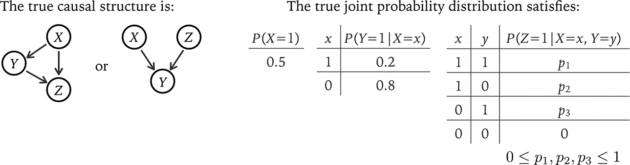
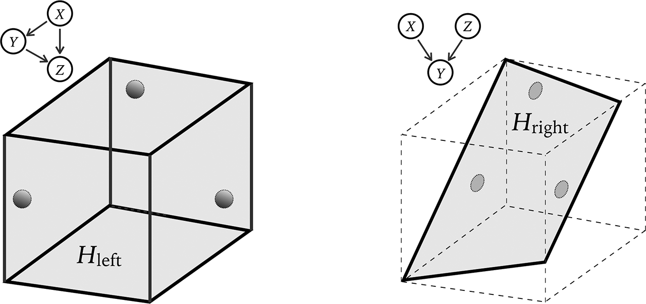
Suppose that we are studying a causal system with three binary variables: X, Y, and Z. We want to know the causal structure among them. We somehow already know for sure that the true causal structure is one of the two depicted in figure 1, where  means that X is an immediate cause of Y. We also already know for sure that the true (yet unknown) joint chance distribution of X, Y, Z satisfies all the conditions listed in the same figure. Those conditions are assumed only to make the case simple and illuminating; no philosophical point hinges on them. It follows from the chain rule in probability calculus that the true joint distribution is fully determined by the three parameters p 1, p 2, and p 3, which are the (unknown) conditional chances of
 given
 , (1, 0), and (0, 1), respectively.Footnote 1 Those three parameters can take any values in the unit interval.
What is known for sure.

Suppose, further, that we know that the (causal) Markov condition applies to the causal system under study—namely, that causation and chance are related to each other in the causal system so that every variable therein is probabilistically independent of its noneffects therein given all of its immediate causes therein. If a variable has no immediate cause in the system, then ‘given all of its immediate causes therein’ is understood trivially as ‘given the truth of a tautology’—namely, conditional independence reduces to unconditional independence. So, if the true causal structure is the one on the right, the Markov condition implies that X is independent of Z. But if the true causal structure is on the left, the Markov condition provably imposes no constraint on parameters p 1, p 2, and p 3.
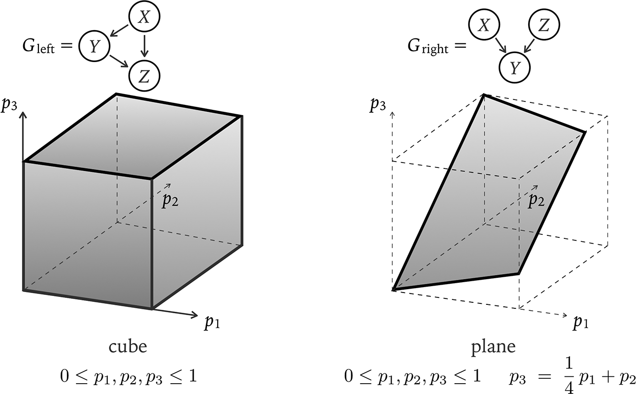
Now, all the possible states of the causal world can be visually represented in figure 2. To be more specific:
Case 1. Suppose that the graph on the left, G left, represents the true causal structure. Then the Markov condition does not rule out any parameter setting. So the possible states can be one-to-one identified with the ordered pairs (G left, (p 1, p 2, p 3)) that satisfy the inequality  , p 2,
 . Those possible states form the unit cube depicted on the left.
Case 2. Suppose that the graph on the right, G right, represents the true causal structure. Then, as noted above, the Markov condition implies that X and Z are independent, which provably translates to this constraint:  . So, in this case, the possible states can be one-to-one identified with the ordered pairs (G right, (p 1, p 2, p 3)) that satisfy the inequality
 , p 2,
 and the equation
 . Those possible states form the trapezoidal zone depicted on the right.
Each possible state represented here is a causal Bayesian network, although we do not really need to give it a formal definition before we proceed further.
Spaces of possible states.

Now we turn to assumptions about data. As is usually the case when data scientists infer causal structures, assume that, for ethical or practical reasons, we can only have access to data that are nonexperimental and nontemporal. Specifically, a nonexperimental, nontemporal data set of sample size n is a data set obtained by observing n instances of the causal system under study, keeping track of all the values of the variables realized in those instances, without experimentation and without information about which variable comes to take a value earlier than which other variable does. Such data sets are also assumed to be generated by observations that are independent and identically distributed—distributed according to the true (but unknown) joint chance distribution. This is known as the IID assumption.
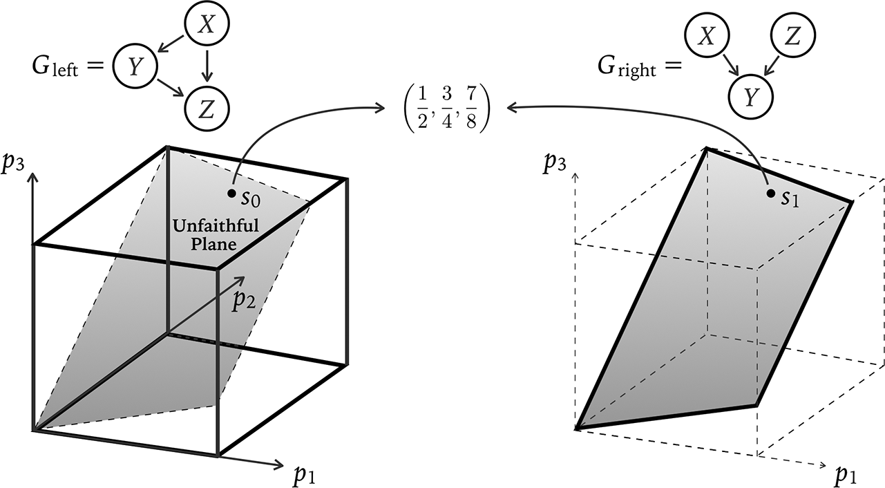
The above fully specifies a causal learning problem, or a problem of choosing between causal structures. To see how hard this problem is, let us have a look at the two possible states indicated in figure 3:  and
 . Those two states disagree on what the true causal structure is. But they are empirically indistinguishable in terms of the kind of data we have access to, even if we have an infinity of such data. For they posit the same joint distribution and, hence, the same sampling distribution over nonexperimental, nontemporal data. Those two possible states, s 0 and s 1, are Cartesian-like skeptical scenarios for each other. Now, think of an arbitrary method that chooses between the two competing causal structures in light of accessible data, or a learning method for short. If a learning method is reliable in one of the two states s 0 and s 1—reliable in the sense of having a high chance of choosing the true causal structure (at a certain sample size)—then it must have an equally high chance of choosing the false one in the other state (at the same sample size). So reliability has to be sacrificed in some states between the Cartesian-like pair s 0 and s 1 and between any other similar pair. The question is which: Which states are those in which reliability should be sacrificed?
Cartesian-like pair of possible states.

The standard practice in data science sacrifices reliability in state s 0; in fact, it sacrifices reliability on the entire trapezoidal plane inscribed in the cube on the left side of figure 3. The question is how we can justify this standard practice. If this practice can be said to follow a kind of Ockham’s razor (because it favors the causal structure on the right, which seems to be simpler than the one on the left), then the question becomes how we can justify this kind of Ockham’s razor.
The above question will not be very interesting unless the underdetermined truths are useful. But causal truths are useful when, for example, we are thinking about making a policy to change the chance of  . It makes sense to adopt a policy to manipulate Y in order to change the chance of
 only if Y is a cause of Z—that is, only if the true causal structure is on the left. For example, consider the policy that forces
 . On the standard account of causal Bayesian networks, this policy would have very different results in the two Cartesian-like states s 0 and s 1. It would increase the chance of
 from 30% to 62.5% in the state on the left, s 0, but it would let the chance of
 remain at 30% in the state on the right, s 1.
To summarize: Useful truths can be underdetermined by the kinds of data we can have access to, even if we have an infinity of such data. The above gives a causal example. Now, there are many learning methods for choosing between those two causal structures in light of nonexperimental, nontemporal data. Which learning methods are the best? Every learning method has to sacrifice reliability in some possible states. Why should we favor the learning methods that sacrifice reliability in the way that follows the standard practice in data science? Those are the questions I would like to address.
3. The Old Solution
The standard solution to the present problem tries to secure reliability in every possible state on the table, but it does so by removing some possible states from the table. That is, it makes an assumption to rule out some possible states and, thereby, narrow down the range of possible states on the table (Spirtes et al. Reference Spirtes, Glymour and Scheines1993; Meek Reference Meek, Besnard and Hanks1995). The most famous such assumption is the (causal) Faithfulness assumption. A precise definition of Faithfulness will be provided when we really need it. What is important for now is the job it does. It basically works in the present case by ruling out the possible states in the trapezoidal plane inscribed in the cube on the left of figure 3—namely, it assumes that the true possible state is not in that trapezoidal plane. That trapezoidal plane will be called the Unfaithful Plane, as indicated in the same figure.
The standard solution makes use of the Faithfulness assumption as follows. It would be great to have a learning method that is reliable uniformly across all possible states on the table at a fixed sample size. Unfortunately, that epistemic ideal is too high to be achievable even with the Faithfulness assumption (Robins et al. Reference Robins, Scheines, Spirtes and Wasserman2003). But, under that assumption, it becomes at least possible to design a learning method that would become reliable as the sample size increases indefinitely in each possible state on the table (Spirtes et al. Reference Spirtes, Glymour and Scheines1993). To be more precise, a learning method M is said to converge stochastically to the truth in a possible state s if, with respect to the sampling distribution generated by the joint chance distribution in s and the IID assumption, the chance for M to identify the truth approaches 1 as the sample size increases indefinitely. A learning method M is said to be statistically consistent with respect to a learning problem 𝒫 if M converges stochastically to the truth in every possible state compatible with what is assumed or taken for granted in learning problem 𝒫. When the range of possible states on the table is narrowed down by adding the Faithfulness assumption—that is, when the Unfaithful Plane is ruled out, there provably exist learning methods that are statistically consistent—statistical consistency is provably achievable.
To be sure, statistical consistency alone does not make a good learning method. The textbook criterion regarding the value of statistical consistency seems, rather, to be as follows:
(The Value of Statistical Consistency) A good learning method for tackling a problem 𝒫 must achieve some epistemic ideals, including at least statistical consistency as a minimal qualification regarding reliability, if it would be great to find the truth among the alternative theories considered in 𝒫 and if statistical consistency is achievable under the assumptions made in 𝒫.
The last “if” clause indicates that, like any epistemic ideal, statistical consistency must be achievable to be worth pursuing. On the standard solution to the present problem, it is the Faithfulness assumption that makes statistical consistency achievable.
So the above is the standard solution. It raises an immediate question: Why should we make the Faithfulness assumption? The standard reply is that we do not need to worry about making the Faithfulness assumption because it is a fairly weak assumption, ruling out only a mathematically negligible set of possible states (Spirtes et al. Reference Spirtes, Glymour and Scheines1993; Meek Reference Meek, Besnard and Hanks1995). To see that it does so, we do not really need a rigorous definition of mathematical negligibility. Indeed, Faithfulness only rules out the Unfaithful Plane, which is a two-dimensional cross-section of the three-dimensional cubic state space on the left of figure 3.
But the appeal to negligibility alone does not suffice to explain why we should make the Faithfulness assumption—or why we should rule out the Unfaithful Plane. For there are many alternative assumptions that also rule out only mathematically negligible sets in the two state spaces. For example, consider the gerrymandered assumption that rules out (i) the state  on the right and (ii) the trapezoidal plane on the left, except for the state
 . This gerrymandered assumption rules out something less than a cross-section of the three-dimensional, cubic state space on the left, and it rules out only a point in the two-dimensional, planar state space on the right. So this gerrymandered assumption is weak enough to rule out only mathematically negligible sets in the two state spaces, although it is already strong enough to make statistical consistency achievable. Then why should we make the Faithfulness assumption rather than the gerrymandered one, or any of the infinitely many alternatives?
Let me paraphrase the question just raised. The decision to design a learning method under the assumption that rules out the Unfaithful Plane amounts to the decision to sacrifice reliability on that plane. But why should we sacrifice reliability on that plane rather than any of the infinitely many alternative negligible regions? The hard problem of theory choice remains unaddressed. We need a new solution.
4. A New Approach
In the absence of the Faithfulness assumption or the like, the underdetermination of truths by data is so severe that even statistical consistency is too high an epistemic ideal to be achievable. Then how should we proceed to evaluate learning methods? My solution is simple: We should not achieve what is unachievable; we only need to, and ought to, achieve the best we can have. Let me explain how to do that.
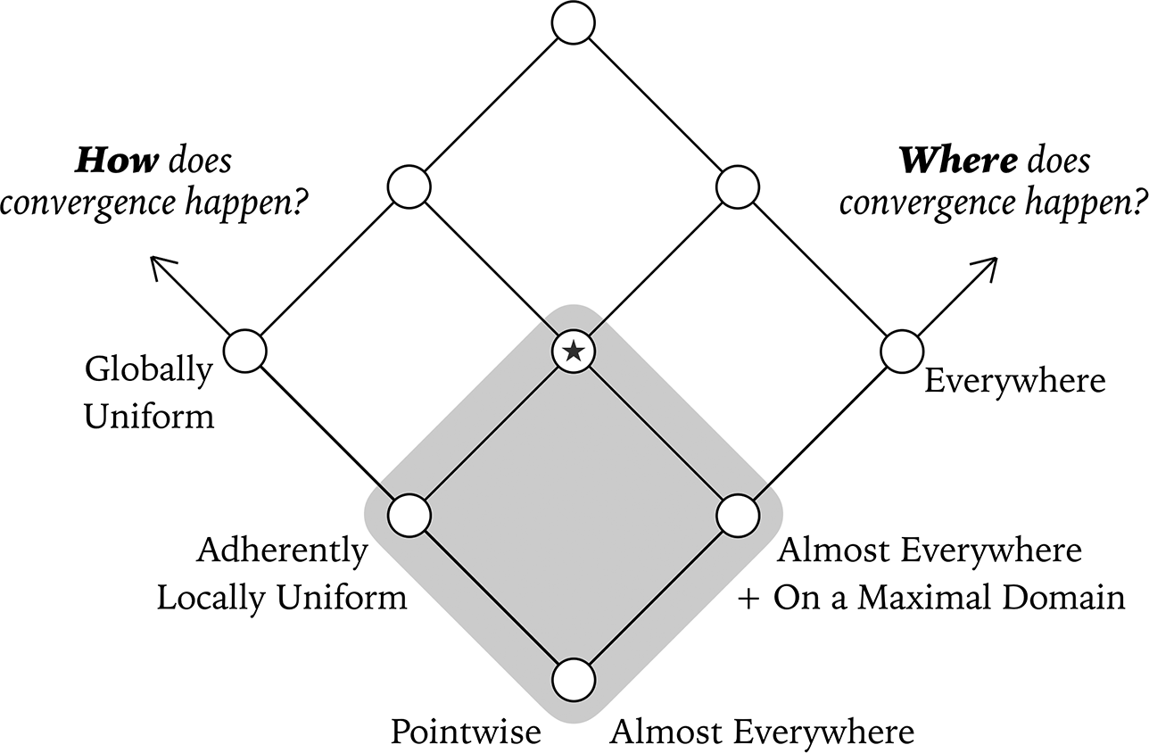
Statistical consistency means having stochastic convergence to the truth everywhere on the state spaces under consideration, and it is only one of the many epistemic ideals regarding reliability. If it is impossible to make it everywhere, we should see whether it is possible to make it at least almost everywhere—pending a good definition of ‘almost everywhere’. If it is possible to achieve at least that much, let us see whether it is possible to achieve more. The guideline, I propose, is to look for what can be achieved and achieve the best we can have.
To implement this idea, have a look at the two-dimensional lattice depicted in figure 4. The two dimensions concern, respectively, the questions of where convergence to the truth happens and how it happens. Each dimension has three modes of convergence to the truth in order of ascending epistemic value, so in combination there are nine joint modes—nine epistemic ideals regarding reliability. To anticipate, “almost everywhere” will be defined quite standardly as in geometry and topology. And “adherently locally uniform convergence” will be defined as a kind of locally uniform convergence that serves as a statistical variant of Nozick’s (1981) adherence condition for knowledge.
Modes of stochastic convergence to the truth.

The modes of convergence mentioned above will be defined soon. Once that is done, we can prove the following result:
Theorem 1. Consider the above causal learning problem, with the IID assumption; the assumption that only nonexperimental, nontemporal data are accessible; and the simplifying assumptions stated in figure 1 (without the causal Faithfulness assumption or the like). Then:
1. Of the nine modes of stochastic convergence to the truth, the ones that are achievable with respect to the present learning problem are exactly those in the shaded area in figure 4. (So the highest achievable epistemic ideal of the nine is the starred mode in the middle.)
2. For every learning method M that tackles the present learning problem, if M achieves the starred mode—“almost everywhere” plus “on a maximal domain” plus “adherently locally uniform”—then M converges stochastically to the truth only in possible states outside of the Unfaithful Plane; that is, M sacrifices convergence to the truth on the entire Unfaithful Plane.
Note that the second part of this result makes a strong claim, applicable to all learning methods tackling the present learning problem. This has an important consequence: to achieve at least the starred mode, which is the best mode of convergence we can have for the present learning problem, it is necessary to sacrifice convergence to the truth on the entire Unfaithful Plane—it is necessary, not a mere option. This result answers the question left by the standard solution.
The way I propose to solve the hard problem of theory choice, or at least the causal instance of this problem, can be summarized by the following argument:
Premise 1. In the lattice depicted in figure 4, if a mode of convergence to the truth is ordered higher, it is a higher epistemic ideal about reliability.
Premise 2. For tackling a learning problem, the best learning methods might have to achieve epistemic ideals of various kinds (e.g., ideals about coherence, unbiasedness, or reliability), but they must at least achieve, of the nine epistemic ideals about reliability in the lattice, the highest achievable one—if such a highest one exists uniquely. (Achieve the best we can have.)
Premise 3. Theorem 1 is true.
Conclusion. So, the best learning methods for tackling the present learning problem must have at least the following properties:
(C1) achieving the starred mode of convergence to the truth (by premises 1 and 2 and the first part of the theorem),
(C2) sacrificing stochastic convergence to the truth on the entire Unfaithful Plane—as if the Faithfulness condition were accepted as true (by C1 and the second part of the theorem).
The rest of this article defines the key concepts in the above theorem, sketches a proof with an explanatory picture, and reports a more general theorem.
5. Definitions
A causal hypothesis H is understood as a set of possible causal states with a topological structure. For example, the cubic hypothesis H left is equipped with the Euclidean topology generated by open balls (fig. 5, left). The trapezoidal hypothesis H right is equipped with the Euclidean topology generated by open discs (fig. 5, right). More formally, I define those topologies standardly in terms of the so-called total variation distance between probability measures, which turns out to generate the Euclidean topology in the present case.Footnote 2 A region in a topological space H is said to be topologically negligible, or nowhere dense, if it is a subset  such that every nonempty open set O of H includes some nonempty open set O′ of H that is disjoint from S. In that case, S has an open “hole” O′ in every open neighborhood O, so it is like a slice of Swiss cheese incredibly full of open holes in H. For example, the Unfaithful Plane is a negligible region in H left, and so is any subset of the Unfaithful Plane. Both the empty set and the singleton {s 1} are negligible regions in H right.
Open sets, which are open balls in the cubic hypothesis H left and open discs in the planar hypothesis H right.

A learning method M is said to converge stochastically to the truth almost everywhere if, for each hypothesis H under consideration, M converges stochastically to the truth in all states in H except on a topologically negligible region of H. Method M is said to converge stochastically to the truth on a maximal domain if no other learning method does on a more inclusive set of possible states.
A learning method M is said to converge stochastically to the truth with global uniformity if, for any (upper bound of error probability)  , there exists a sample size n such that, given any sample size greater than or equal to n, there is a chance at least
 for M to output the truth in all possible states under consideration (i.e., all possible states contained in
 ). Global uniformity would be great to have if it could be achieved, for it would allow us to control the sample size to ensure any desired level of reliability—ensured for all the states in
 simultaneously. But this epistemic ideal is too high to be achievable, simply because it implies statistical consistency, namely, stochastic convergence to the truth everywhere. Well, if we cannot make it globally, let us see whether we can make it at least locally.
A learning method M is said to converge stochastically to the truth with adherent local uniformity if, for any hypothesis H under consideration (be it the cube H left or the plane H right) and for any state  in which M converges to the truth stochastically, s has an open neighborhood N in H (where N is an open ball in the cube H left or an open disc in the plane H right) such that:
Method M has stochastic convergence to the truth uniformly on neighborhood  ; namely, for any (upper bound of error probability)
 , there exists a sample size n such that, given any sample size greater than or equal to n, there is a chance at least
 for M to output the truth in each state contained in neighborhood
 .
This means that, for any possible state s in which M converges to the truth stochastically, a sufficiently large sample size can stably secure a high chance for M to output the truth—having a high reliability secured not just in s but stably secured under small perturbations of the joint chance distribution true in s. This is a kind of locally uniform convergence. It is also a statistical variant of Nozick’s (Reference Nozick1981) adherence condition for knowledge, which says roughly that, if the truth one believes in were true in a slightly different way, then one would still believe in it—one’s belief would “adhere” to the truth. This finishes the definitions of all the concepts involved in theorem 1.
6. Sketch of Proof
Theorem 1 has two parts. Part 1, like many existence results, has a tedious proof. It is an immediate corollary of a more general result in my joint work with Jiji Zhang (see Lin and Zhang Reference Lin and Zhang2019, theorem 1).
But part 2 has a revealing, pictorial proof that explains why the achievement of at least (a) “almost everywhere” plus (b) “on a maximal domain” plus (c) “adherent local uniformity” forces a learning method to sacrifice convergence to the truth on the Unfaithful Plane. In fact, a plus c alone forces that.
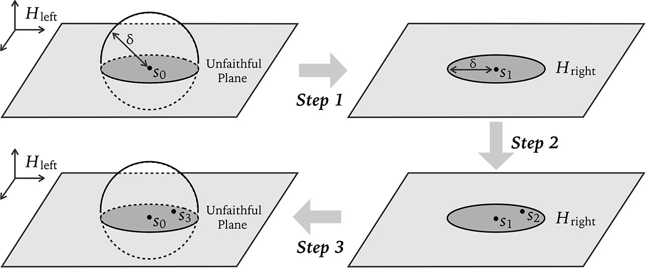
Proof of Part 2 of Theorem 1. Let M be an arbitrary learning method for the above learning problem that achieves these two modes of stochastic convergence to the truth: “almost everywhere” and “adherent local uniformity.” I will omit ‘stochastic’ when writing the proof. Suppose, for reductio, that M converges to the truth in a state s 0 on the Unfaithful Plane, which is embedded in state space H left. By adherent local uniformity, M converges to the truth uniformly on some open ball B δ(s 0) centered at s 0 with radius  , as depicted in the upper left part of figure 6. From state s 0, let us construct states s 1, s 2, and s 3 in three steps, which follow the flow in figure 6.
Step 1. Take state  and replace the causal structure therein by G right to obtain state
 , retaining the same chance distribution. So we have constructed state s 1, which is in hypothesis H right.
Step 2. Recall that δ is the radius of the open ball B δ(s 0) mentioned above. Use the same radius to construct an open disc  centered at s 1. Since D δ(s 1) is an open disc in H right, M must converge to the truth H right in some state in D δ(s 1). For otherwise M would fail to converge to the truth on a certain open set (i.e., D δ(s 1)) in topological space H right, which contradicts the supposition that M converges to the truth almost everywhere in each hypothesis. Now, choose a state s 2 in the open disc D δ(s 1) in which M converges to the true hypothesis H right. Let P′ be the chance distribution in s 2. So
 .
Step 3. Take state  and replace the causal structure therein by G left to obtain state
 , retaining the same chance distribution. So we have constructed state s 3, which is in hypothesis H left. This finishes the three-step construction.
State s 3 has two notable properties. First, s 3 is less than δ away from s 0, because s 2 is less than δ away from s 1 (by construction). Second, in state s 3 we have that M converges to H right (a falsehood), because s 3 has the same chance distribution as s 2 (by construction) and because in s 2 we have that M converges to H right (by construction). To sum up, s 3 is both a state in the open ball  and a state in which M fails to converge to the truth. It follows that M fails to converge to the truth uniformly on the open ball B δ(s 0)—contradiction. QED
Proof that we must sacrifice convergence to the truth on the Unfaithful Plane.

7. Closing: Report of a General Result
The above theorem can be generalized as follows. A directed acyclic graph G, understood as a causal structure, is said to entail a conditional independence statement if that statement holds with respect to every joint chance distribution P such that G and P jointly satisfy the (causal) Markov condition. Let ℐ(G) denote the set of the conditional independence statements that G entails. Similarly, let ℐ(P) denote the set of the conditional independence statements that hold with respect to P. Then the Markov condition can be equivalently reformulated as

A causal Bayesian network, which is also called a (possible) causal state (of the world), is an ordered pair (G, P) that satisfies the Markov condition. The Faithfulness condition strengthens the Markov condition by requiring that

The Faithfulness condition rules out the Unfaithful Plane discussed above. A causal Bayesian network satisfying Faithfulness is called a faithful causal state. The Faithfulness assumption says that the actual causal state is faithful. Faithfulness has some weaker variants (for a review and comparison, see Zhang [Reference Zhang2013]). A learning method for the present purposes is a function that maps each data set of a finite sample size to a causal hypothesis taking this form: “The true causal structure is Markov equivalent to G,” where the Markov equivalence between two graphs G and G′ is defined by  . Such a method is a method for learning the Markov equivalence structure of the true (but unknown) causal Bayesian network. Then the preceding theorem can be generalized as follows; it is an immediate corollary of the main result of Lin and Zhang (Reference Lin and Zhang2019, theorem 1):
Theorem 2. Let 𝒫 be a problem of learning the Markov equivalence structure of the true (but unknown) causal Bayesian network. Suppose that problem 𝒫 makes only the following assumptions: that the true causal Bayesian network is defined on a finite, fixed set of categorical variables; that only nonexperimental, nontemporal data are accessible; and that data are IID. (So there is no assumption of Faithfulness or any of its variants). Then:
1. Of the nine modes of stochastic convergence to the truth, the ones that are achievable with respect to problem 𝒫 are exactly those in the shaded area in figure 4. (So the highest achievable epistemic ideal of the nine is the starred mode in the middle.)
2. For every learning method M that tackles problem 𝒫, if M achieves the starred mode in figure 4, then M has this convergence property: converging stochastically to the truth in every faithful causal state and sacrificing convergence to the truth in every causal state that shares the same chance distribution with some faithful causal state.
It is a standard practice of causal inference in data science to design and employ causal learning methods that satisfy at least the convergence property specified in clause 2, at least when data are assumed to be IID, nonexperimental, and nontemporal. This standard practice is justified by the above theorem and the guideline developed in this article: Look for what can be achieved, and achieve the best we can have.