



1. Introduction
One of the remarkable features of compressible turbulent mixing layers is the significantly reduced growth rate as the convective Mach number (
 $M_c$
) increases (Papamoschou & Roshko Reference Papamoschou and Roshko1988; Freund, Lele & Moin Reference Freund, Lele and Moin2000; Pantano & Sarkar Reference Pantano and Sarkar2002), which has important implications for various applications including rocket engines and hypersonic vehicles (Abada, Abada & El-hirtsi Reference Abada, Abada and El-Hirtsi2020). This suppression process is accompanied by a fundamental change in the nature of large-scale turbulent structures: at low Mach numbers the flow is dominated by spanwise-oriented Kelvin–Helmholtz (K–H) rollers; with increasing compressibility it transitions to elongated large-scale streaky structures (LSSs) that closely resemble structures observed in wall-bounded turbulence (Mungal Reference Mungal1995; Messersmith & Dutton Reference Messersmith and Dutton1996; Pirozzoli et al. Reference Pirozzoli, Bernardini, Marié and Grasso2015; Wang, Wang & Chen Reference Wang, Wang and Chen2022). These large-scale structures have been shown to carry a significant fraction of the turbulent kinetic energy (TKE) and Reynolds shear stress, and play a key role in the transportation of heat, mass and momentum (Marusic et al. Reference Marusic, McKeon, Monkewitz, Nagib, Smits and Sreenivasan2010; Lee & Sung Reference Lee and Sung2011; Yu et al. Reference Yu, Dong, Guo, Tang, Yuan and Xu2024; Wang et al. Reference Wang, Guo, Wang and Chen2025). Investigating the dynamics of these structures not only enhances our understanding of compressible turbulence but also contributes to the development of more accurate turbulence models for high-speed flow simulations.
The spatial scale of the elongated LSSs is one of the key issues in turbulence research and has been extensively investigated in wall-bounded turbulent flows. Their characteristic scales can be measured from instantaneous flow fields or determined by spatio-temporal statistical quantities, including the two-point correlations of streamwise velocity fluctuations (Ganapathisubramani et al. Reference Ganapathisubramani, Hutchins, Hambleton, Longmire and Marusic2005; Hutchins & Marusic Reference Hutchins and Marusic2007; Lee & Sung Reference Lee and Sung2013; Bross, Scharnowski & Kähler Reference Bross, Scharnowski and Kähler2021), proper orthogonal decomposition (Baltzer, Adrian & Wu Reference Baltzer, Adrian and Wu2013; de Silva et al. Reference de Silva, Chandran, Baidya, Hutchins and Marusic2020) and the premultiplied energy spectrum (Monty et al. Reference Monty, Stewart, Williams and Chong2007; Mathis, Hutchins & Marusic Reference Mathis, Hutchins and Marusic2009). In wall-bounded turbulence, the LSSs are typically classified according to their streamwise extent into two types: large-scale motions, with streamwise lengths of the order of
 $2\delta$
–
 $3\delta$
, and very-large-scale motions or ‘superstructures’, with sizes ranging from
 $10\delta$
to
 $50\delta$
(Ganapathisubramani, Longmire & Marusic Reference Ganapathisubramani, Longmire and Marusic2003; Hutchins & Marusic Reference Hutchins and Marusic2007; Dennis & Nickels Reference Dennis and Nickels2011; Lee & Sung Reference Lee and Sung2011). Here,
 $\delta$
denotes the boundary-layer thickness, the channel half-height or the pipe radius, depending on the flow configuration.
The effects of compressibility on the spatial scales of large-scale structures in wall-bounded turbulence have been far less studied, and the reported results vary considerably and qualitatively. Smits et al. (Reference Smits, Spina, Alving, Smith, Fernando and Donovan1989) performed hot-wire measurements in a Mach 2.9 turbulent boundary layer and found that the streamwise length scale of mass-flux autocorrelations in supersonic flows is about half that in incompressible flows. Smits & Dussauge (Reference Smits and Dussauge2006) further suggested that the streamwise length scales decrease significantly with increasing Mach number, whereas the spanwise scales remain nearly unchanged with variations in Mach and Reynolds numbers. On the other hand, Pirozzoli & Bernardini (Reference Pirozzoli and Bernardini2011), through direct numerical simulations (DNS) of a Mach 2.0 turbulent boundary layer, reported that the two-point correlations of streamwise velocity fluctuations agree well with the low-speed data of Hutchins & Marusic (Reference Hutchins and Marusic2007) at similar Reynolds numbers, indicating that both streamwise and spanwise length scales are only weakly affected by compressibility and Reynolds number variations. Other studies, however, have suggested that compressibility tends to increase the streamwise scale of large-scale structures. Ganapathisubramani, Clemens & Dolling (Reference Ganapathisubramani, Clemens and Dolling2006) conducted particle image velocimetry measurements of a Mach 2.0 turbulent boundary layer, and the two-point correlations of streamwise velocity fluctuations revealed that the streamwise length scales are approximately four times larger than those in incompressible cases reported in the literature, while the spanwise scales are also somewhat larger. Ringuette, Wu & Martín (Reference Ringuette, Wu and Martín2008) investigated a Mach 3 turbulent boundary layer and observed instantaneous low-speed streaky structures as long as
 $100\delta$
in the streamwise direction, far exceeding the
 $20\delta$
observed by Hutchins & Marusic (Reference Hutchins and Marusic2007), though their instantaneous fields were also reconstructed using Taylor’s hypothesis. More recently, Bross et al. (Reference Bross, Scharnowski and Kähler2021) conducted experimental studies of turbulent boundary layers with Mach numbers ranging from 0.3 to 3.0. Using multi-point correlation and spectral analysis methods, they found that the streamwise scales of the large-scale structures in supersonic cases are slightly larger than those in subsonic cases, while the spanwise scales increase significantly with Mach number. They attributed the wide discrepancies among existing studies to differences in boundary conditions, flow configurations and measurement techniques, emphasising that obtaining reliable compressible turbulent-boundary-layer data remains a formidable challenge for both experiments and simulations.
The above review of wall-bounded turbulence indicates that, due to the inherent complexity of compressible wall-bounded turbulence, there is still no definitive conclusion regarding how compressibility affects the spatial scale of elongated large-scale structures. To address this issue in a simpler yet physically meaningful configuration, the present study focuses on compressible turbulent mixing layers, which represent the simplest form of shear turbulence in nature (Pope Reference Pope2000). Previous studies have shown that streamwise large-scale structures in compressible free-shear flows share notable similarities with those observed in the outer region of wall-bounded turbulence (Pirozzoli et al. Reference Pirozzoli, Bernardini, Marié and Grasso2015; Wang et al. Reference Wang, Wang and Chen2022, Reference Wang, Guo, Wang and Chen2024, Reference Wang, Guo, Wang and Chen2025), implying that insights gained from the mixing layer may also shed light on the influence of compressibility in wall-bounded turbulence.
However, quantitative investigations of the elongated large-scale structures in compressible mixing layers remain very limited. In an experimental study of a spatially developing mixing layer, Mungal (Reference Mungal1995) observed that the large-scale structures become elongated in the streamwise direction at moderate convective Mach numbers (
 $M_c \approx 0.8$
). Similarly, Messersmith & Dutton (Reference Messersmith and Dutton1996) reported that the size of streamwise-oriented large structures in compressible mixing layers generally increases with increasing compressibility. DNS by Pirozzoli et al. (Reference Pirozzoli, Bernardini, Marié and Grasso2015) of a spatially developing mixing layer at
 $M_c \approx 0.45$
revealed that the streamwise velocity field organises into large-scale low- and high-speed streaks, with the spanwise integral scales being comparable to those in boundary layers, although the streamwise scale was not explicitly quantified. In our recent study (Wang et al. Reference Wang, Wang and Chen2022), we performed DNS of compressible mixing layers at convective Mach numbers
 $M_c = 0.2$
,
 $0.8$
and
 $1.8$
. It was found that, as
 $M_c$
increases, the streamwise integral length scale increases significantly, whereas the spanwise integral scale remains nearly constant. Furthermore, in the self-similar stage of the mixing layer, both the streamwise and spanwise integral scales, when normalised by the vorticity thickness, remain nearly invariant. Unlike in wall-bounded turbulence, existing studies on mixing layers consistently suggest that compressibility tends to increase the streamwise scale of the large-scale structures.
The reduction of turbulence intensity and the growth rate of compressible mixing layers at high convective Mach numbers (
 $M_c$
) has long been a central issue in compressible free-shear turbulence research (Vreman, Sandham & Luo Reference Vreman, Sandham and Luo1996; Pantano & Sarkar Reference Pantano and Sarkar2002; Jahanbakhshi & Madnia Reference Jahanbakhshi and Madnia2016; Arun et al. Reference Arun, Sameen, Srinivasan and Girimaji2019). From the perspective of TKE transport, Vreman et al. (Reference Vreman, Sandham and Luo1996) and Pantano & Sarkar (Reference Pantano and Sarkar2002) demonstrated that the suppression primarily originates from the weakened coupling between pressure and strain, which limits the pressure–strain redistribution among velocity components and consequently reduces turbulence production. This mechanism has since been widely recognised as the dominant explanation for the compressibility-induced suppression of turbulence. However, a clear connection between the TKE transport term and the evolution of elongated large-scale structures in compressible mixing layers remains lacking.
In addition, it is worth noting that existing numerical simulations of compressible turbulent mixing layers have so far been limited to relatively low convective Mach numbers, typically not exceeding
 $M_c \approx 2.0$
(Pantano & Sarkar Reference Pantano and Sarkar2002; Vaghefi & Madnia Reference Vaghefi and Madnia2015; Vadrot, Giauque & Corre Reference Vadrot, Giauque and Corre2021; Matsuno & Lele Reference Matsuno and Lele2021; Wang et al. Reference Wang, Wang and Chen2022). This Mach-number range is substantially lower than that encountered in many practical high-speed flow applications, such as rocket exhaust plumes and hypersonic propulsion systems, where much stronger compressibility effects are present (Abada et al. Reference Abada, Abada and El-Hirtsi2020). In contrast, recent numerical studies of compressible turbulent boundary layers have successfully reached significantly higher free-stream Mach numbers, up to
 $M_\infty \approx 6$
or beyond, and have provided important insights into the role of compressibility in high-speed wall-bounded turbulence (Lagha et al. Reference Lagha, Kim, Eldredge and Zhong2011; Toki et al. Reference Toki, Sousa, Chen, Camillo, Wagner and Scalo2025). Extending numerical investigations of compressible mixing layers to higher convective Mach numbers is therefore essential for assessing the validity of physical mechanisms identified at moderate
 $M_c$
and for clarifying the influence of strong compressibility on the evolution and organisation of large-scale structures in free-shear flows.
The present study aims to elucidate how compressibility influences the spatial scales and evolution of elongated large-scale structures in compressible turbulent mixing layers. DNS are performed for convective Mach numbers up to
 $M_c = 5.0$
, which is significantly higher than the maximum values (around
 $M_c \approx 2.0$
) reported in previous studies. The increase in Mach number considerably slows down the evolution of large-scale structures, allowing for a clearer examination of their development process. In this work, we not only quantify the variation of the spatial scales of elongated large-scale structures with
 $M_c$
, but also analyse their evolution mechanism from the perspective of TKE transport.
The remainder of this paper is organised as follows. Section 2 describes the numerical methods, flow configurations and analysis procedures. Section 3 presents the main results, including the compressibility effects on the spatial scales, temporal evolution and energy transfer associated with the elongated large-scale structures. Finally, the conclusions are summarised in § 4.
2. Direct numerical simulation of compressible mixing layers
We study a compressible temporally evolving mixing layer of a calorically perfect ideal gas governed by the following dimensionless Navier–Stokes equations in the conservative form (Wang et al. Reference Wang, Shi, Wang, Xiao, He and Chen2012, Reference Wang, Wang and Chen2022):
 \begin{align} \frac {\partial \rho }{\partial t} + \frac {\partial (\rho u_k)}{\partial x_k} = 0, \\[-28pt] \nonumber \end{align}
 \begin{align} \frac {\partial (\rho u_i)}{\partial t} + \frac {\partial (\rho u_k u_i)}{\partial x_k} = -\frac {\partial p}{\partial x_i} + \frac {1}{\textit{Re}}\frac {\partial \sigma _{ik}}{\partial x_k}, \\[-28pt] \nonumber \end{align}
 \begin{align} \frac {\partial E}{\partial t} + \frac {\partial [(E+p)u_{\!j}]}{\partial x_{\!j}} = \frac {1}{\alpha }\frac {\partial }{\partial x_k} \left ( \kappa \frac {\partial T}{\partial x_k} \right ) + \frac {1}{\textit{Re}}\frac {\partial (u_{\!j}\sigma _{jk})}{\partial x_k}, \\[-28pt] \nonumber \end{align}
 \begin{align} p = \rho T/(\gamma M^2), \\[0pt] \nonumber \end{align}
where
 $u_i$
,
 $\rho$
,
 $p$
and
 $T$
are the instantaneous velocity component, density, pressure and temperature, respectively. Here, the viscous stress
 $\sigma _{ik}$
is defined as
 \begin{align} \sigma _{ik} = 2\mu {\unicode{x1D64E}}_{ik}- \frac {2\mu \varTheta }{3}\delta _{ik}, \end{align}
in which
 ${\unicode{x1D64E}}_{ik}=( \partial u_i /\partial x_k + \partial u_k/\partial x_i)/2$
is the strain rate tensor and
 $\varTheta = \partial u_k/\partial x_k$
is the velocity divergence or dilatation. The total energy per unit volume
 $ E$
is given by
 \begin{align} E=\frac {p}{\gamma -1} + \frac {1}{2}\rho u_iu_i. \end{align}
Moreover, the temperature-dependent viscosity coefficient
 $ \mu$
and thermal conductivity coefficient
 $ \kappa$
are specified by Sutherland’s law (Sutherland Reference Sutherland1893).
The variables in the governing equations of compressible turbulence have already been normalised by a set of reference scales, including the reference length
 $L_r$
, velocity
 $U_r$
, density
 $\rho _r$
, pressure
 $p_r=\rho _rU_r^2$
, temperature
 $T_r$
, energy per unit volume
 $\rho _rU_r^2$
, viscosity
 $\mu _r$
and thermal conductivity
 $\kappa _r$
(Samtaney, Pullin & Kosović Reference Samtaney, Pullin and Kosović2001; Wang et al. Reference Wang, Shi, Wang, Xiao, He and Chen2012; Yu et al. Reference Yu, Fouxon, Wang, Li, Yuan, Mao and Mond2023). There are three reference governing parameters: the reference Reynolds number
 $Re = \rho _rU_rL_r/\mu _r$
, the reference Mach number
 $M=U_r/c_r$
and the reference Prandtl number
 $\textit{Pr} = \mu _rC_{\!p}/\kappa _r$
, which is assumed to be equal to 0.7. In addition, the reference speed of sound is defined by
 $c_r = \sqrt {\gamma \textit{RT}_r}$
, where
 $R$
is the specific gas constant. Here,
 $\gamma = C_{\!p}/C_v$
is the ratio of specific heat at constant pressure
 $C_{\!p}$
to that at constant volume
 $C_v$
, which is assumed to be equal to 1.4. Consistent with the calorically perfect gas assumption, both
 $C_{\!p}$
and
 $C_v$
are treated as constants. The parameter
 $ \alpha$
is defined as
 $ \alpha = \textit{Pr} Re(\gamma -1)M^2$
.
A hybrid compact-weighted essentially non-oscillatory (WENO) scheme (Wang et al. Reference Wang, Wang, Xiao, Shi and Chen2010; Liu et al. Reference Liu, Wang, Shi, Chen and He2019) is applied for numerical simulations of a compressible temporally evolving mixing layer. The hybrid scheme combines an eighth-order compact finite-difference scheme (Lele Reference Lele1992) in smooth regions and a seventh-order WENO scheme (Balsara & Shu Reference Balsara and Shu2000) in shock regions. The shock regions are identified by spatial points with highly negative local dilatation as defined by
 $\varTheta \lt 3.0\varTheta _{\textit{rms}}$
(Samtaney et al. Reference Samtaney, Pullin and Kosović2001), where
 $ \varTheta _{\textit{rms}}$
is the root-mean-square of dilatation. The numerical simulations essentially resolve flow fields above the Kolmogorov length scale, while the discontinuities around shock waves are captured by the WENO scheme.
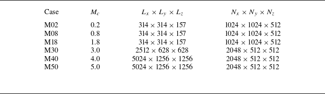
Summary of computation parameters. Here
 $L_x$
,
 $L_y$
and
 $L_z$
denote computational domain lengths measured in terms of initial momentum thickness
 $\delta _\theta ^0$
, while
 $N_x$
,
 $N_y$
and
 $N_z$
denote the corresponding number of grid points.

Schematic of the temporally evolving shear layer. The black solid curve represents the mean velocity profile, while the contour map displays the instantaneous temperature in the
 $ x{-}y$
plane. The red dashed rectangles denote the boundaries of the sponge layers at the vertical boundary.

The numerical simulations have been performed for six different convective Mach numbers,
 $M_c=$
0.2, 0.8, 1.8, 3.0, 4.0, 5.0. The convective Mach number
 $ M_c$
is defined as
 $ M_c=\Delta U/(2c_\infty )$
, where
 $ c_\infty$
is the speed of sound in the free stream and
 $ \Delta U$
is the free-stream velocity difference across the shear layer. Figure 1 is a schematic of the flow configuration considered in the present work. The coordinate system
 $ x$
,
 $ y$
and
 $ z$
refers to the streamwise, vertical and spanwise directions, respectively, and
 $ u$
,
 $ v$
and
 $ w$
denote the instantaneous velocity components in the corresponding directions. The computational domains are designed to ensure that the large-scale structures are fully captured. Computational domain sizes and grid resolutions for different
 $ M_c$
are listed in table 1. Here,
 $L_x$
,
 $L_y$
and
 $L_z$
denote the streamwise, vertical and spanwise domain dimensions, normalised by the initial momentum thickness
 $\delta _\theta ^0$
. Boundary conditions are periodic in the homogeneous streamwise and spanwise directions. To allow periodic configuration in the vertical direction, the mean streamwise velocity is initialised by a hyperbolic tangent profile with two shear layers (one is located at the middle and the other at the boundary of the transverse direction):
 \begin{align} \begin{split} \widetilde {u} = \frac {1}{2}\Delta U \bigg [ \text{tanh}\bigg (\frac {y }{2C_\delta \delta _\theta ^0}\bigg ) -\text{tanh}\bigg (\frac {y+L_y/2}{2C_\delta \delta _\theta ^0}\bigg ) -\text{tanh}\bigg (\frac {y-L_y/2}{2C_\delta \delta _\theta ^0}\bigg ) \bigg ], \end{split} \end{align}
where
 $ C_\delta$
is an adjustment constant to account for the effect of compressibility (Vaghefi Reference Vaghefi2014; Vaghefi & Madnia Reference Vaghefi and Madnia2015; Wang et al. Reference Wang, Wang and Chen2022). Specifically,
 $C_\delta$
is calibrated using the bisection method such that the momentum thickness calculated from the initial field matches the prescribed initial momentum thickness
 $\delta _\theta ^0$
. The momentum thickness
 $ \delta _\theta$
is computed by (Vreman et al. Reference Vreman, Sandham and Luo1996)
 \begin{align} \begin{split} \delta _\theta = \frac {1}{\rho _\infty \Delta U^2}\int _{-\infty }^{+\infty } \overline {\rho } \big ( \Delta U/2-\widetilde {u} \big )\big ( \Delta U/2+\widetilde {u} \big ){\rm d}y, \end{split} \end{align}
where
 $ \widetilde {u}$
and
 $ \overline {\rho }$
are the Favre average of streamwise velocity and the Reynolds average of density, respectively. The Reynolds average of a variable
 $ \phi$
is denoted by
 $ \overline {\phi }$
, while the Reynolds fluctuation is denoted as
 $ \phi ^\prime =\phi -\overline {\phi }$
. The Favre average of a variable
 $ \phi$
is denoted by
 $ \widetilde {\phi }=\overline {\rho \phi }/\overline {\rho }$
, and its Favre fluctuation is denoted as
 $ \phi ^{\prime \prime }=\phi -\widetilde {\phi }$
. The spatial averaging is performed along the homogeneous
 $ x$
and
 $ z$
directions. To enhance statistical stability, ensemble averaging is performed over six independent realisations with different initial random perturbation for each convective Mach number. A numerical diffusion zone is applied near the vertical boundary, which can reduce the intensity of possible disturbances at the vertical boundary such that there is a negligible effect on the mixing layer (Reckinger, Livescu & Vasilyev Reference Reckinger, Livescu and Vasilyev2016; Wang et al. Reference Wang, Wang and Chen2022). The mean vertical and spanwise velocities are set to zero. The initial temperature
 $ {T}$
is obtained from the Busemann–Crocco relationship (Ragab & Wu Reference Ragab and Wu1989; Arun et al. Reference Arun, Sameen, Srinivasan and Girimaji2019) for compressible shear layers:
 \begin{align} \begin{split} {T} = 1+\frac {1}{2}(\gamma -1)M_c^2(1-\widetilde {u}^2). \end{split} \end{align}
The pressure field is uniform and the density field is acquired from the ideal gas equation of state. To accelerate the transition to turbulence, a spatially correlated perturbation velocity field obtained by the digital filter method (Klein, Sadiki & Janicka Reference Klein, Sadiki and Janicka2003; Vaghefi Reference Vaghefi2014; Wang et al. Reference Wang, Wang and Chen2022) is superposed on mean velocities. The filtering length in each direction is chosen as the initial vorticity thickness
 $ \delta _\omega$
, computed by (Vreman et al. Reference Vreman, Sandham and Luo1996)
 \begin{align} \delta _\omega =\frac {\Delta U}{({\rm d}\widetilde {u}/{\rm d}y)_{\textit{max}}}. \end{align}
The TKE (
 $ K=\overline {\rho u_i^{\prime \prime }u_i^{\prime \prime }}/2$
) transport equation for a compressible temporally evolving mixing layer can be written as (Pantano & Sarkar Reference Pantano and Sarkar2002)
 \begin{align} \begin{split} \frac {\partial K}{\partial t} + \frac {\partial K\widetilde {u}_k}{\partial x_k} = D + P + \varPhi - \epsilon + \varSigma . \end{split} \end{align}
Here,
 $ D$
is the spatial diffusion of TKE,
 $ P$
is the production term,
 $ \varPhi$
is the pressure-dilatation term,
 $ \epsilon$
is the viscous dissipation term and
 $ \varSigma$
is the mass flux coupling term. These terms are defined as
 \begin{align} {D} &= - \frac {\partial }{\partial x_k}\bigg ( \frac {1}{2}\overline {\rho u_i^{\prime \prime }u_i^{\prime \prime }u_k^{\prime \prime }} + \overline {p^\prime u^{\prime \prime }_i}\delta _{ik} - \frac {1}{\textit{Re}}\overline {\sigma ^\prime _{ik}u^{\prime \prime }_i}\bigg ), \\[-12pt]\nonumber \end{align}
 \begin{align} {P} &= - \overline {\rho u_i^{\prime \prime }u_k^{\prime \prime }}\frac {\partial \widetilde {u}_i}{\partial x_k}, \\[-12pt]\nonumber \end{align}
 \begin{align} {\epsilon } &= -\frac {1}{\textit{Re}}\overline {\sigma ^\prime _{ik}\frac {\partial u^{\prime \prime }_i}{\partial x_k}}, \\[-12pt]\nonumber \end{align}
 \begin{align} {\varPhi } &= \overline {p^\prime \frac {\partial u^{\prime \prime }_i}{\partial x_i}}, \\[-12pt]\nonumber \end{align}
 \begin{align} {\varSigma } &= \overline {u_i^{\prime \prime }}\bigg (\frac {1}{\textit{Re}}\frac {\partial \overline {\sigma }_{ik}}{\partial x_k} - \frac {\partial \overline {p}}{\partial x_i}\bigg ). \end{align}
Among the above terms, the diffusion, production and dissipation terms are dominant in the transport of TKE
 $ K$
. The mass flux coupling term is negligibly small after ensemble averaging (Pantano & Sarkar Reference Pantano and Sarkar2002). The transport equation for the TKE components
 $ {K}_i$
can be simply obtained by avoiding summation convention over repeated indices
 $ i$
in (2.11) and (2.12), and the corresponding transport terms are
 $ {D}_i$
,
 $ {P}_i$
,
 $ {\epsilon }_i$
,
 $ {\varPhi }_i$
and
 $ {\varSigma }_i$
(Pantano & Sarkar Reference Pantano and Sarkar2002; Arun et al. Reference Arun, Sameen, Srinivasan and Girimaji2019). The pressure–strain term,
 $ {\varPhi }_i$
, becomes dominant for redistributing energy between three components of TKE.
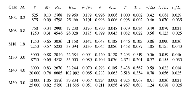
Several key non-dimensional flow parameters corresponding to the self-similar period at the centreline are presented in table 2. The statistics are functions of
 $ y$
and normalised time
 $ \tau = t\Delta U/\delta _\theta ^0$
. The Reynolds numbers based on the momentum thickness
 $ \textit{Re}_\theta$
and the vorticity thickness
 $ \textit{Re}_\omega$
are defined as
 \begin{align} \begin{split} \textit{Re}_\theta = \frac {\rho _\infty \Delta U \delta _\theta }{\mu _\infty },\quad \textit{Re}_\omega = \frac {\rho _\infty \Delta U \delta _\omega }{\mu _\infty },\ \end{split} \end{align}
respectively. The initial momentum thickness Reynolds number is
 $ \textit{Re}_\theta = 320$
. The self-similar period is carefully determined by analysing the time evolution of the mean velocity, Reynolds stresses and integrated transfer terms of TKE. The turbulent Mach number
 $ M_t={\sqrt {\overline {u_i^{\prime \prime } u_i^{\prime \prime }}}}/{c}$
ranges from 0.1 to 1.0, where
 $ c$
is the average speed of sound. The lowest value (
 $ M_t = 0.1$
) corresponds to the quasi-incompressible case at
 $ M_c = 0.2$
, while the highest value (
 $ M_t = 1.0$
) occurs at
 $ M_c = 5.0$
. To the best of our knowledge, this upper limit of
 $ M_t$
significantly exceeds the strongest compressibility levels previously reported in numerical simulations (Pantano & Sarkar Reference Pantano and Sarkar2002; Arun et al. Reference Arun, Sameen, Srinivasan and Girimaji2019; Wang et al. Reference Wang, Wang and Chen2022). As the convective Mach number
 $M_c$
increases, the mean density
 $\overline {\rho }$
at the mixing-layer centre decreases continuously, while the mean temperature
 $\overline {T}$
increases significantly due to enhanced compressibility heating. The root mean square of density fluctuations
 $\rho _{\textit{rms}}$
first increases and then decreases with
 $M_c$
, reaching its maximum around
 $M_c=3.0$
. In contrast, the root mean square of temperature fluctuations
 $T_{\textit{rms}}$
increases monotonically with
 $M_c$
.
Simulation parameters at the beginning and end of the self-similar period. The values of
 $M_t$
,
 $ \overline {\rho }$
,
 $ \rho _{\textit{rms}}$
,
 $ \overline {T}$
,
 $ T_{\textit{rms}}$
,
 $\eta$
,
 $ l_x$
and
 $ l_z$
are obtained at
 $ y = 0$
. The density and temperature are normalised by their values in the free stream.

The integral length scales in the streamwise direction
 $ (l_x)$
and spanwise direction
 $ (l_z)$
are defined as
 \begin{align} \begin{split} l_x = \int _{0}^{L_x/2}\mathcal{R}_{xu}(r_x){\rm d}r_x,\quad l_z = \int _{0}^{L_z/2}\mathcal{R}_{zu}(r_z){\rm d}r_z, \end{split} \end{align}
respectively. Here,
 $ \mathcal{R}_{xf}$
and
 $ \mathcal{R}_{zf}$
are the two-point correlation of a variable
 $ f$
in streamwise and spanwise directions, respectively, and these correlations are specifically computed at the centreplane of the mixing layer (
 $ y = 0.0$
). They are defined as
 \begin{align} \begin{split} \mathcal{R}_{xf}(r_x) = \frac {\langle f^{\prime \prime }(x,0,z)f^{\prime \prime }(x+r_x,0,z) \rangle }{f_{\textit{rms}}^2}, \quad \mathcal{R}_{zf}(r_z) = \frac {\langle f^{\prime \prime }(x,0,z)f^{\prime \prime }(x,0,z+r_z) \rangle }{f_{\textit{rms}}^2}, \ \end{split} \end{align}
where
 $ \langle \ \rangle$
stands for ensemble average. The integral length scales in the streamwise and spanwise directions are sufficiently small compared with the length of the computational domain, ensuring that the self-similar growth of LSSs is not confined. In terms of the local Kolmogorov length scale
 $ \eta =( {\mu ^3}/{(\rho ^3\epsilon )} )^{1/4}$
, the resolution parameter
 $ \eta /\Delta x$
is in the range
 $ 0.56 \leqslant \eta /\Delta x \leqslant 1.24$
at the centreline, where
 $ \Delta x$
is the grid length in each direction, indicating that the resolution of the present simulations is fine enough to resolve the smallest scales in the flow, as given in table 2. A detailed description and a comprehensive validation of the DNS can be found in recent works by the authors (Wang et al. Reference Wang, Wang and Chen2022, Reference Wang, Guo, Wang and Chen2024, Reference Wang, Guo, Wang and Chen2025).
3. Results and discussion
3.1. Suppression of mixing-layer growth rate
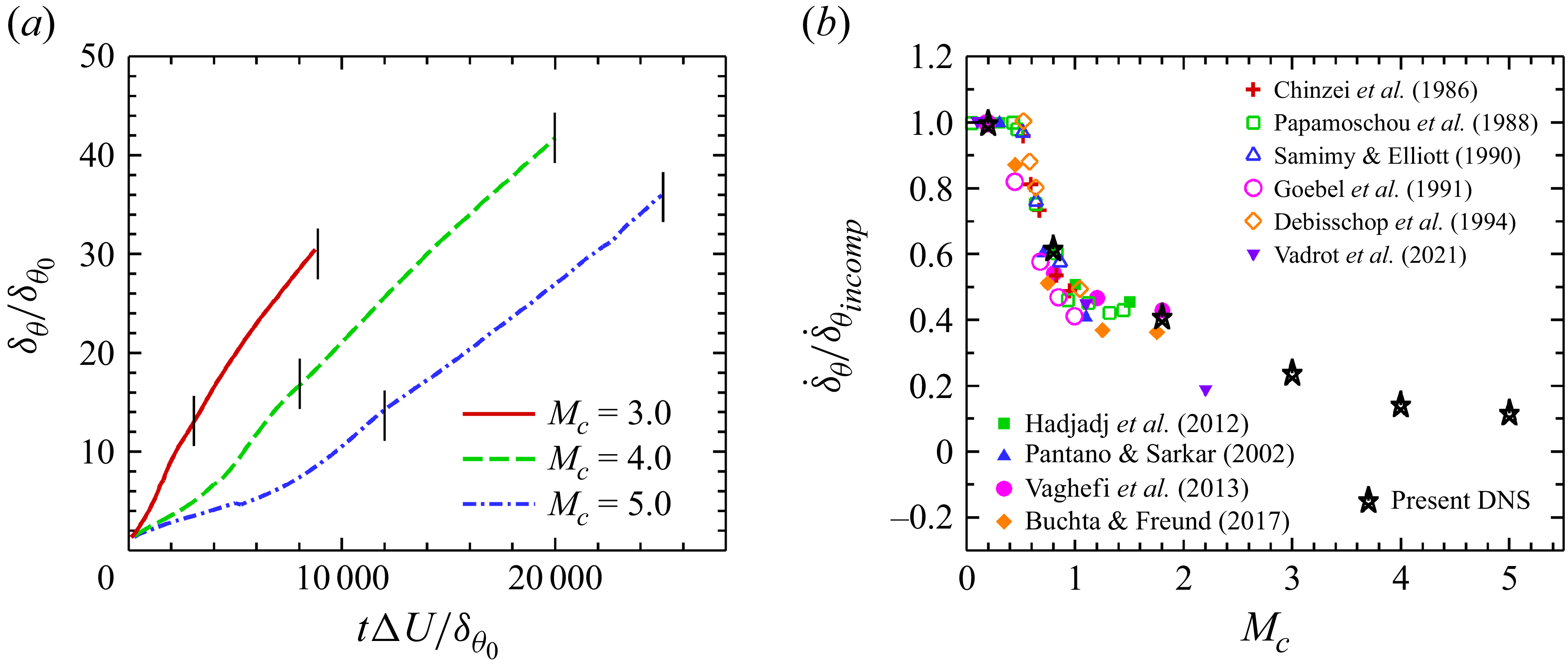
The time evolution of the momentum thickness, normalised by its initial value (
 $ \delta _\theta ^0$
), is shown in figure 2(a) for
 $ M_c =3.0$
,
 $ 4.0$
and
 $ 5.0$
. It can be observed that the duration of the transition regime increases significantly with
 $M_c$
. At
 $M_c = 5.0$
, the transition period exceeds
 $ \tau = 10\,000$
, which is approximately ten times longer than that at
 $M_c = 3.0$
. For both
 $M_c = 4.0$
and
 $5.0$
, the momentum thickness exhibits a distinct linear growth during the initial transition phase (
 $\tau \lt 3000$
for
 $M_c = 4.0$
;
 $\tau \lt 6000$
for
 $M_c = 5.0$
). Interestingly, the corresponding growth rate during this early transition phase is lower than that in the self-similar regime.
(a) Time evolution of normalised momentum thickness for
 $ M_c =3.0$
,
 $ 4.0$
and
 $ 5.0$
, where the vertical line segments mark the self-similar time periods. (b) Comparison of linear growth rates at different
 $ M_c$
with various numerical and experimental results.

Figure 2. Long description
Panel A: A line graph shows the time evolution of normalized momentum thickness for convective Mach numbers 3.0, 4.0, and 5.0. The x-axis represents the dimensionless time (tΔU/δθ0) and the y-axis represents the normalized momentum thickness (δθ/δθ0). The graph includes three lines: a solid red line for Mc = 3.0, a dashed green line for Mc = 4.0, and a dash-dotted blue line for Mc = 5.0. Vertical line segments mark the self-similar time periods. Panel B: A scatter plot compares the linear growth rates at different convective Mach numbers with various numerical and experimental results. The x-axis represents the convective Mach number (Mc) and the y-axis represents the normalized growth rate (δθ/δθincomp). The plot includes data points from multiple studies, each represented by different symbols and colors, and a series of black stars representing the present direct numerical simulation (DNS) results.
The normalised self-similar growth rates are presented in figure 2(b), where
 $ \dot {\delta }_{\textit{incomp}}$
is the growth rate of the quasi-incompressible case
 $ M_c=0.2$
in our simulations. For comparison, numerical (Pantano & Sarkar Reference Pantano and Sarkar2002; Rossmann, Mungal & Hanson Reference Rossmann, Mungal and Hanson2002; Hadjadj, Yee & Sjögreen Reference Hadjadj, Yee and Sjögreen2012; Vaghefi et al. Reference Vaghefi, Nik, Pisciuneri and Madnia2013; Buchta & Freund Reference Buchta and Freund2017; Vadrot et al. Reference Vadrot, Giauque and Corre2021) and experimental (Chinzei et al. Reference Chinzei, Masuya, Komuro, Murakami and Kudou1986; Papamoschou & Roshko Reference Papamoschou and Roshko1988; Samimy & Elliott Reference Samimy and Elliott1990; Goebel & Dutton Reference Goebel and Dutton1991; Debisschop, Chambers & Bonnet Reference Debisschop, Chambers and Bonnet1994) data available in the literature are also shown. It can be seen that the growth rate data reported in previous studies for
 $M_c \lesssim 2.0$
exhibit a considerable scattered behaviour. Based on a broader survey and analysis of the growth-rate data reported in the literature (Pantano & Sarkar Reference Pantano and Sarkar2002; Arun et al. Reference Arun, Sameen, Srinivasan and Girimaji2019; Matsuno & Lele Reference Matsuno and Lele2021; Vadrot et al. Reference Vadrot, Giauque and Corre2021), this scatter appears to arise from several factors. First, the determination of the self-similar period in compressible mixing layers is not straightforward and may vary among different studies, which can affect the extracted growth rates (Vadrot et al. Reference Vadrot, Giauque and Corre2021). Second, different definitions of the mixing-layer thickness are often employed, including the momentum thickness, vorticity thickness and visual thickness, which may lead to different trends with increasing Mach number (Papamoschou & Roshko Reference Papamoschou and Roshko1988). Third, the reported results are obtained from different flow configurations, such as temporally or spatially developing mixing layers, planar or annular geometries (Freund et al. Reference Freund, Lele and Moin2000). Since these factors are often not strictly distinguished when growth-rate data from different studies are compared, the resulting datasets may exhibit a noticeable scatter.
In the present study, the growth rate is evaluated using the momentum thickness. In DNS, the evaluation of the vorticity thickness (see (2.10)) relies on the maximum gradient of the mean velocity profile and therefore involves only a very limited number of grid points near the mixing-layer centre, which makes it difficult to obtain statistically stable results. By contrast, the momentum thickness (see (2.8)) is defined as an integral quantity across the entire mixing layer and generally provides a more statistically robust measure.
It is also worth noting that most of the available studies focus on convective Mach numbers below approximately
 $M_c \approx 2.0$
. The present direct numerical simulation extends the analysis to significantly higher convective Mach numbers, up to
 $ M_c = 5.0$
, which allows the evolution of the growth rate in the high-Mach-number regime to be examined. As can be seen in figure 2(b), the growth rate of the momentum thickness continues to decrease from
 $ M_c = 1.8$
to
 $ 5.0$
. At
 $ M_c = 5.0$
,
 $ \dot {\delta } / \dot {\delta }_{\textit{incomp}} = 0.12$
, which is approximately one-tenth of the incompressible value. These results indicate that the growth rate of the momentum thickness does not reach saturation, in contrast to the conclusions of Freund et al. (Reference Freund, Lele and Moin2000) and Barone, Oberkampf & Blottner (Reference Barone, Oberkampf and Blottner2006), who reported saturation below
 $M_c = 2.0$
. Since the momentum thickness is directly related to the mean density, its continuous decrease with increasing
 $M_c$
leads to the persistent reduction of the growth rate. According to the definition of the momentum thickness (see (2.8)), it is closely related to the mean density. As the convective Mach number
 $M_c$
increases, the mean density decreases significantly (see table 2), which directly leads to the continuous reduction of the momentum thickness.
3.2. Evolution of LSSs in instantaneous flow fields
Figures 3–5 show the temporal evolution of the very long
 $ u^{\prime \prime }$
structures in the instantaneous flow fields on the central
 $ x{-}z$
plane at
 $ M_c=3.0, 4.0$
and
 $ 5.0$
, respectively. Each figure displays the entire computational domain, with the spatial extent normalised by the vorticity thickness
 $\delta _\omega$
evaluated at each instant. Since
 $\delta _\omega$
increases over time, the normalised domain size shown in the figures decreases accordingly. For clarity, only the negative values of
 $ u^{\prime \prime }$
are visualised. Based on the full dataset, the temporal evolution of the large-scale structures can be divided into three distinct stages: (i) a streak formation stage, (ii) a streak instability stage and (iii) a fully developed turbulent stage. The three snapshots shown in the figures are selected to be representative of these stages.
Instantaneous fields of
 $ u^{\prime \prime }\lt 0.0$
in the central
 $ x{-}z$
plane for the case with
 $ M_c=3.0$
: (a)
 $ \tau =200$
, (b)
 $ \tau =1250$
and (c)
 $ \tau =7500$
.

Instantaneous fields of
 $ u^{\prime \prime }\lt 0.0$
in the central
 $ x{-}z$
plane for the case with
 $ M_c=4.0$
: (a)
 $ \tau =2000$
, (b)
 $ \tau =6250$
and (c)
 $ \tau =17500$
.

Instantaneous fields of
 $ u^{\prime \prime }\lt 0.0$
in the central
 $ x{-}z$
plane for the case with
 $ M_c=5.0$
: (a)
 $ \tau =5000$
, (b)
 $ \tau =10\,000$
and (c)
 $ \tau =22\,500$
.

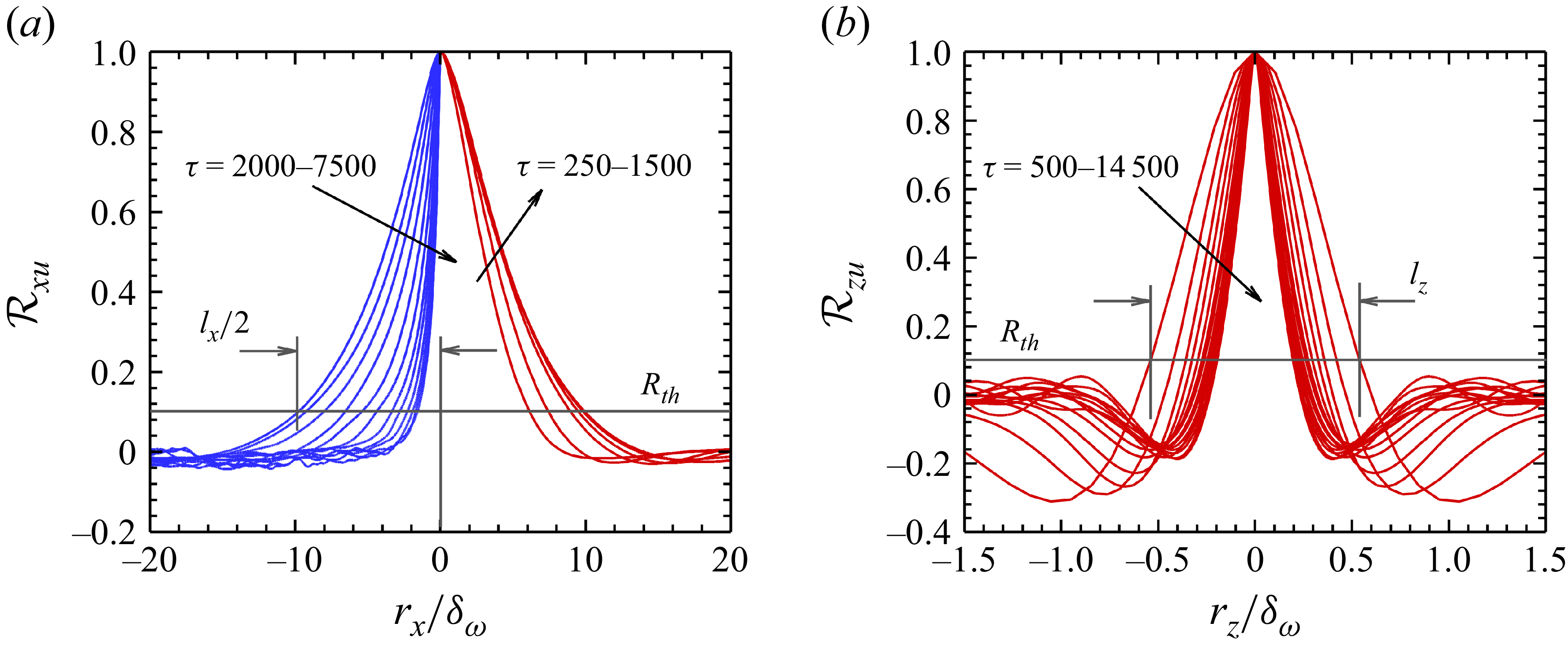
Two-point correlations of the streamwise velocity fluctuations at
 $M_c=4.0$
: (a) streamwise correlation
 $R_{xu}$
(
 $\tau =250$
–
 $1500$
on the right,
 $\tau =2000$
–
 $7500$
on the left, only half shown owing to symmetry) and (b) spanwise correlation
 $R_{zu}$
(
 $\tau =500$
–
 $14\,500$
). All separations are normalised by the vorticity thickness
 $\delta _\omega$
.

Figure 6. Long description
Two graphs depict the streamwise and spanwise correlations of streamwise velocity fluctuations in compressible turbulent mixing layers. Panel A: A line graph shows the streamwise correlation of streamwise velocity fluctuations. The horizontal axis is labeled r_x/delta_omega and ranges from −20 to 20. The vertical axis is labeled R_xu and ranges from −0.2 to 1.0. The graph includes multiple lines in blue and red, representing different time intervals (tau = 2000−7500 for blue lines and tau = 250−1500 for red lines). Key labels include l_x/2 and R_th. Panel B: Another line graph shows the spanwise correlation of streamwise velocity fluctuations. The horizontal axis is labeled r_z/delta_omega and ranges from −1.5 to 1.5. The vertical axis is labeled R_zu and ranges from −0.4 to 1.0. The graph includes multiple red lines representing different time intervals (tau = 500−14500). Key labels include l_z and R_th.
(i) Streak growth stage.
-
In this stage (figures 3 a, 4 a and 5 a), low-speed regions continuously merge to form elongated, streak-like structures with smooth edges. At
 $M_c = 3.0$
, individual streaks extend over approximately half of the computational domain, corresponding to about
$80\delta _\omega$
. At
$M_c = 4.0$
, most low-speed streaks span nearly the entire domain length (
$\sim 100\delta _\omega$
), while at
$M_c = 5.0$
, their streamwise extent clearly exceeds the computational domain (
$\gt 80\delta _\omega$
). The morphology of the
$u^{\prime \prime }$
structures in this stage closely resembles that of the low-speed streaks in the viscous sublayer of wall-bounded turbulence (Moin & Kim Reference Moin and Kim1982; Schoppa & Hussain Reference Schoppa and Hussain2002).


(ii) Streak breakdown stage.
-
Once the streaks reach a certain amplitude (figures 3 b, 4 b and 5 b), they begin to exhibit meandering and oscillatory motions due to intrinsic instabilities. Their fragmentation results in shorter streamwise extents, while pronounced small-scale structures emerge along the streak interfaces owing to strong local shear between adjacent high- and low-speed regions. With increasing compressibility, this inner shear-layer instability is significantly suppressed (Wang et al. Reference Wang, Guo, Wang and Chen2024), leading to a marked reduction of small-scale motions near the interfaces at
$M_c = 5.0$
.

(iii) Fully developed turbulent stage.
-
In this stage (figures 3 c, 4 c and 5 c), the large-scale structures are populated with abundant small-scale motions, leading to highly complex interface morphologies. Despite the variations in
$M_c$
, the overall shape and characteristic scale of the large-scale structures remain remarkably similar.

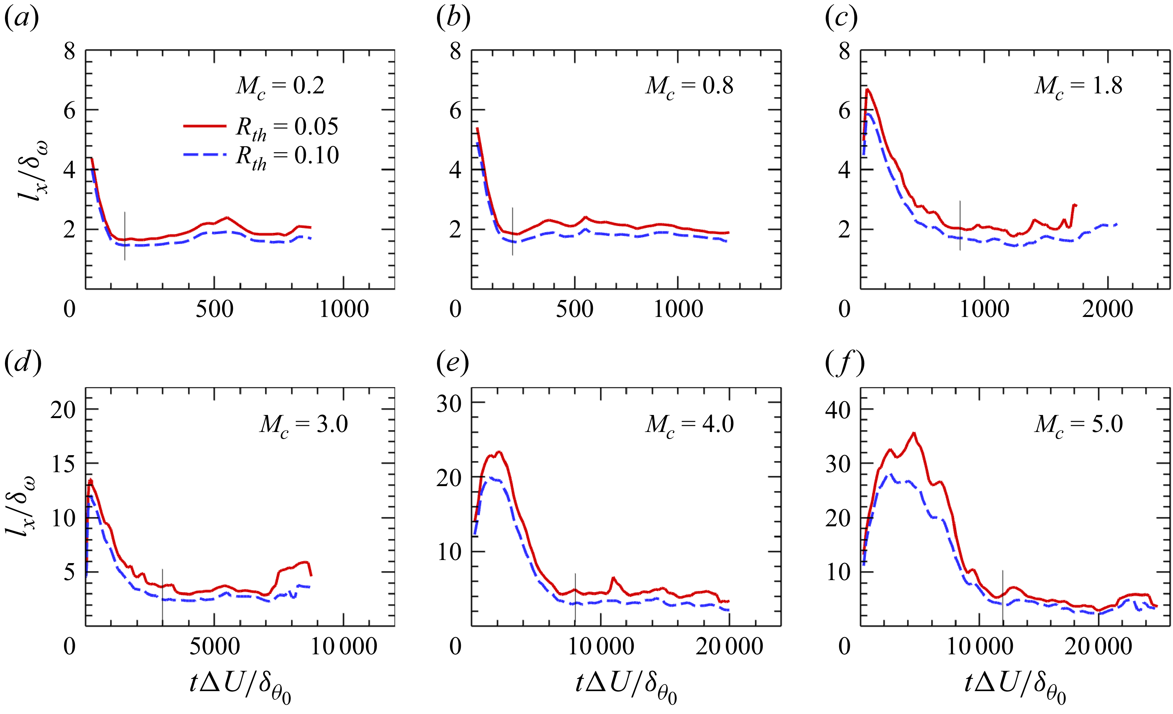
Time evolution of the normalised streamwise length scale
 $ l_x/\delta _\omega$
extracted with different threshold
 $ R_{\textit{th}} = 0.05,\ 0.1$
. The vertical line segments indicate the onset of the statistically steady stage of
 $ l_x/\delta _\omega$
: (a)
 $ M_c=0.2$
, (b)
 $ M_c=0.8$
, (c)
 $ M_c=1.8$
, (d)
 $ M_c=3.0$
, (e)
 $ M_c=4.0$
and (f)
 $ M_c=5.0$
.

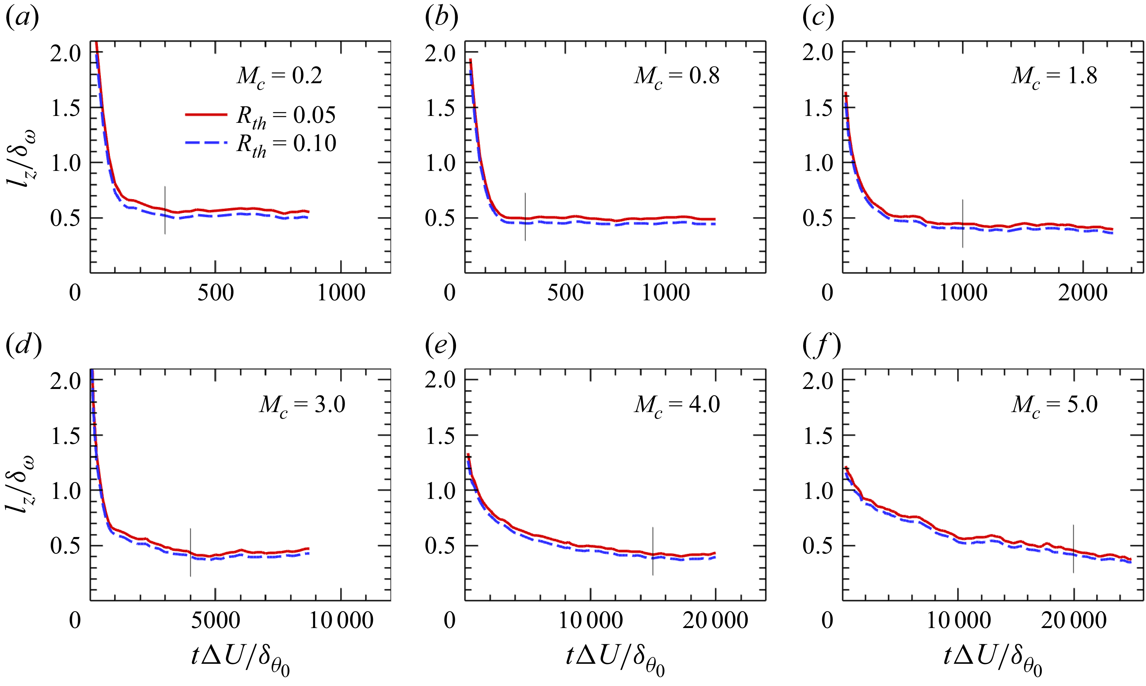
Time evolution of the normalised spanwise length scale
 $ l_z/\delta _\omega$
extracted with different threshold
 $ R_{\textit{th}} = 0.05,\ 0.1$
. The vertical line segments indicate the onset of the statistically steady stage of
 $ l_z/\delta _\omega$
: (a)
 $ M_c=0.2$
, (b)
 $ M_c=0.8$
, (c)
 $ M_c=1.8$
, (d)
 $ M_c=3.0$
, (e)
 $ M_c=4.0$
and (f)
 $ M_c=5.0$
.

3.3. Spatial scales of LSSs
Figure 6 presents the streamwise two-point autocorrelation of streamwise velocity fluctuations,
 $R_{xu}(r_x)$
, evaluated at the centreplane of the temporally developing mixing layer for case
 $ M_c=4.0$
. The spatial separation
 $r_x$
is normalised by the instantaneous vorticity thickness
 $\delta _\omega$
. The evolution of large-scale structures is illustrated by comparing two distinct time intervals:
 $\tau = 250 {-} 1500$
(showing only the right half,
 $r_x / \delta _w \geqslant 0$
) and
 $\tau = 2000 {-} 7500$
(showing only the left half,
 $r_x / \delta _w \leqslant 0$
), leveraging the inherent symmetry of
 $R_{xu}$
about
 $r_x / \delta _w = 0$
. During the initial development phase (
 $\tau = 250$
–
 $1500$
), the
 $R_{xu}$
profile broadens significantly, indicating a rapid growth in the streamwise length scale of the emerging large-scale structures. In the subsequent evolution phase (
 $\tau = 2000$
–
 $7500$
), the correlation profile gradually narrows and eventually stabilises, indicating that the characteristic streamwise extent of the large-scale structures decreases from its maximum and reaches a statistically stationary, saturated state. This sequential broadening, narrowing and stabilisation of the autocorrelation function directly captures the dynamic evolution of the streamwise extent of large-scale coherent structures in the temporally developing mixing layer. The spanwise length of large-scale coherent structures exhibits monotonic reduction from initial development until saturation, as quantified by the spanwise velocity correlation
 $R_{zu}(r_z/\delta _\omega )$
in figure 6(b). The stabilisation of both
 $ R_{xu}$
and
 $ R_{zu}$
provides a clear indication that the flow has reached the self-similar state, and they scale well on the vorticity thickness
 $ \delta _\omega$
.
To determine the characteristic length scales from the two-point correlation functions of the streamwise velocity fluctuations, a nominal threshold value
 $R_{\textit{th}}$
must be specified, as shown in figure 6. Because the extracted length scales can be sensitive to the chosen threshold (Lee & Sung Reference Lee and Sung2011), we report results obtained using two representative values,
 $R_{\textit{th}}=0.05$
and
 $0.1$
, to verify the robustness of our conclusions. Figures 7 and 8 present the normalised streamwise
 $ l_x/\delta _\omega$
and spanwise
 $ l_z/\delta _\omega$
length scales at different
 $ M_c$
. As expected, decreasing the threshold
 $R_{\textit{th}}$
yields larger values of both
 $ l_x/\delta _\omega$
and
 $ l_z/\delta _\omega$
. Moreover, the streamwise length scale exhibits increasing fluctuations as
 $R_{\textit{th}}$
decreases, whereas the spanwise length scale is nearly unaffected. Two factors account for this behaviour. First, the streamwise scale is intrinsically much larger than the spanwise scale; hence, at large separations the correlation naturally becomes weaker, which is reflected in the stronger anti-correlated region of
 $R_{zu}$
compared with the milder anti-correlation in
 $R_{xu}$
. Second, because the computational domain size is fixed, the number of valid statistical samples decreases as the separation distance increases. Although we repeated the simulations up to six times to improve statistical convergence, the fluctuations in the
 $ l_x/\delta _\omega$
curve did not noticeably diminish despite the substantial computational effort.
For the streamwise length scale
 $l_x/\delta _\omega$
, as shown in figure 7, all cases exhibit a similar trend:
 $l_x$
first increases with time, then decreases and finally stabilises within a range of
 $1.5\delta _\omega$
–
 $5.0\delta _\omega$
. This temporal behaviour is consistent with the evolution of the instantaneous
 $u''$
fields discussed earlier. At
 $M_c=0.2$
and
 $0.8$
, the initial growth stage is not clearly resolved because the increase occurs too rapidly within the current sampling interval. With increasing
 $M_c$
, the growth and decay of
 $l_x$
become progressively slower, and the time required for
 $l_x$
to reach its final equilibrium value is substantially delayed. For example, at
 $M_c=0.2$
and
 $0.8$
,
 $l_x$
quickly relaxes to about
 $2\delta _\omega$
within
 $t\Delta U/\delta _{\theta 0}\approx 1000$
, whereas at
 $M_c=3.0$
the stabilisation is postponed until
 $t\Delta U/\delta _{\theta 0}\approx 6000$
, and at
 $M_c=5.0$
it occurs only after
 $t\Delta U/\delta _{\theta 0}\gt 12\,000$
. Regarding the peak values, a strong dependence on
 $M_c$
is observed. At low
 $M_c$
(
 $M_c=0.2$
–0.8), the maximum
 $l_x$
is only a few times
 $\delta _\omega$
. At
 $M_c=3.0$
,
 $l_x$
reaches about
 $14\delta _\omega$
, while at
 $M_c=5.0$
the peak grows dramatically to nearly
 $35\delta _\omega$
before decaying towards its asymptotic value. This indicates that higher compressibility not only slows down the temporal development of the streaks but also amplifies their streamwise elongation to unprecedented scales.
The spanwise length scale
 $l_z/\delta _\omega$
, as shown in figure 8, exhibits a much weaker dependence on
 $M_c$
compared with
 $l_x$
. In all cases,
 $l_z$
decreases monotonically from the beginning, indicating that the initial condition prescribes an overly large spanwise scale. For low and moderate Mach numbers (
 $M_c \leqslant 3.0$
),
 $l_z$
decreases rapidly and quickly reaches a nearly constant value of about
 $0.4\delta _\omega$
. At higher Mach numbers, however, the decay becomes substantially slower and the attainment of a stable value is significantly delayed relative to
 $l_x$
. At
 $M_c=4.0$
, a quasi-equilibrium stage appears only after
 $\tau \gt 15\,000$
, with the asymptotic value again around
 $0.4\delta _\omega$
. At
 $M_c=5.0$
,
 $l_z$
continues to decrease throughout the simulation, approaching
 $0.4\delta _\omega$
by
 $\tau =25\,000$
, but without reaching a clear stabilisation stage.
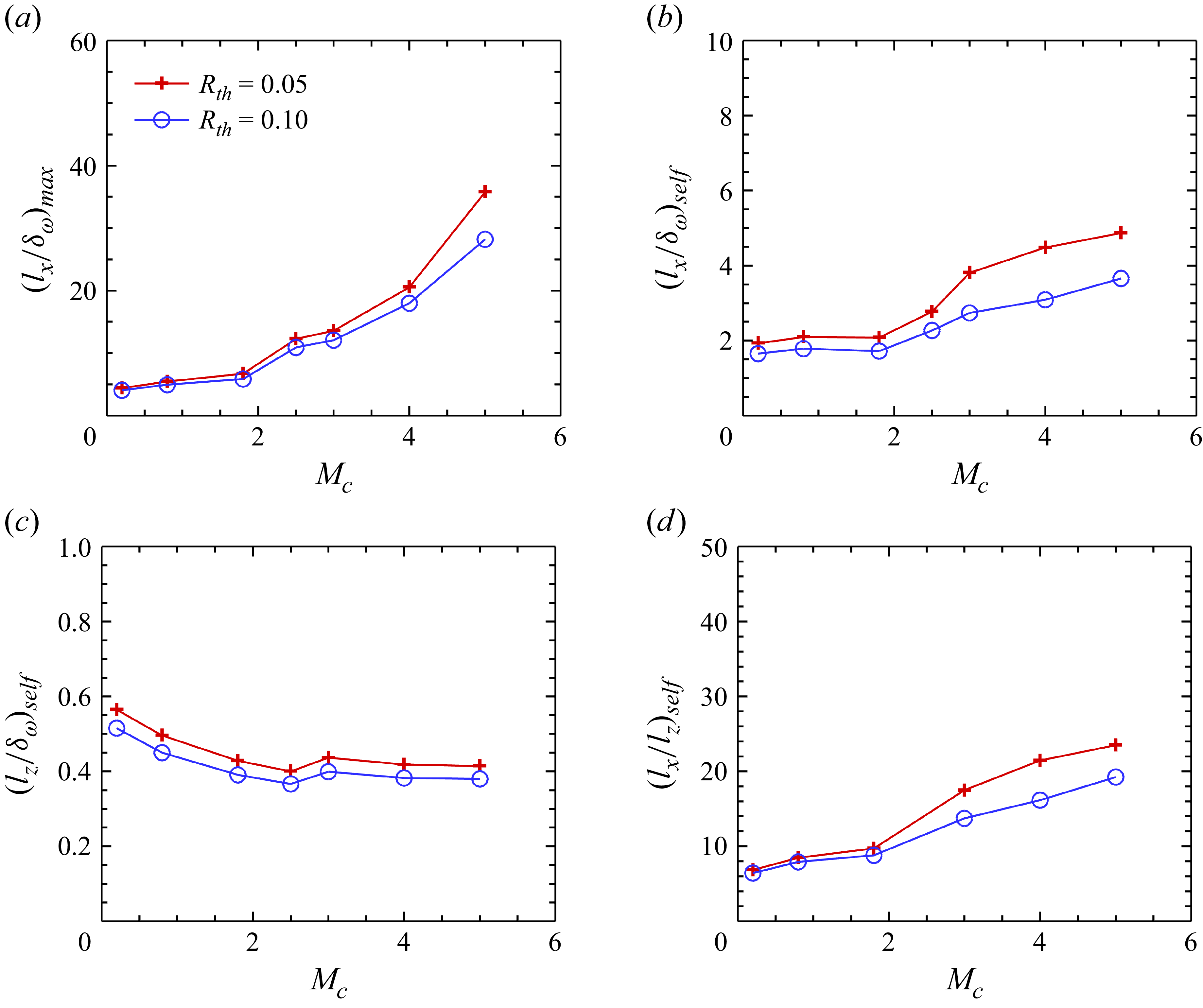
(a) Maximum streamwise length scale,
 $(l_x/\delta _\omega )_{max }$
, as a function of convective Mach number
 $M_c$
. Time-averaged (b) streamwise length scale
 $(l_x/\delta _\omega )_{\textit{self}}$
and (c) spanwise length scale
 $(l_z/\delta _\omega )_{\textit{self}}$
during the statistically steady stage as a function of convective Mach number
 $M_c$
. (d) Ratio of the streamwise and spanwise length scales
 $(l_x/l_z)_{\textit{self}}$
.

Figure 9(a) shows the variation of the maximum streamwise scale,
 $ (l_x/\delta _\omega )_{\textit{max}}$
, with the convective Mach number
 $ M_c$
. Although the correlation threshold has a significant impact, it is clear that as
 $ M_c$
increases,
 $ (l_x/\delta _\omega )_{\textit{max}}$
grows rapidly. This behaviour highlights the significant effect of compressibility on the persistence of elongated streamwise structures. With increasing
 $ M_c$
, the suppression of inner shear-layer instabilities allows streaks to remain coherent for longer periods, thereby enabling the formation of increasingly long streamwise structures before breakdown occurs.
Figures 9(b) and 9(c) show the time-averaged streamwise and spanwise scales of the large-scale structures,
 $(l_x/\delta _\omega )_{\textit{self}}$
and
 $(l_z/\delta _\omega )_{\textit{self}}$
, during the statistically steady stage, respectively. The periods at which
 $l_x$
and
 $l_z$
reach a steady stage differ, and these periods are indicated by black vertical lines in figures 7 and 8. For
 $M_c = 5.0$
,
 $l_z$
does not exhibit a clearly defined steady stage; thus, for consistency, we conservatively compute the time average using data for
 $\tau \gt 20\,000$
. The time-averaged streamwise scale,
 $({l_x}/{\delta _\omega })_{\textit{self}}$
, exhibits a much weaker dependence on
 $M_c$
compared with the maximum value
 $({l_x}/{\delta _\omega })_{max }$
. Although
 $({l_x}/{\delta _\omega })_{\textit{self}}$
also increases with
 $M_c$
, its growth is relatively modest at low Mach numbers, remaining around
 $2\delta _\omega$
. A more pronounced increase is observed for
 $M_c\gt 1.8$
, and at
 $M_c = 5.0$
,
 $({l_x}/{\delta _\omega })_{\textit{self}}$
reaches approximately
 $4\delta _\omega$
. In contrast, the time-averaged spanwise scale,
 $(l_z/\delta _\omega )_{\textit{self}}$
, decreases monotonically with increasing convective Mach number
 $M_c$
. At low to moderate
 $M_c \leqslant 1.8$
, the decrease is relatively pronounced, after which it stabilises around
 $0.4\delta _\omega$
.
The ratio of the streamwise and spanwise length scales is shown in figure 9(d). Since
 $(l_z/\delta _\omega )_{\textit{self}}$
decreases only slightly with increasing
 $M_c$
, the variation of
 $(l_x/l_z)_{\textit{self}}$
closely follows that of
 $(l_x/\delta _\omega )_{\textit{self}}$
. The ratio increases monotonically with
 $M_c$
, reaching values as high as about 25 at
 $M_c=5.0$
for
 $R_{\textit{th}}=0.05$
. This indicates that with increasing
 $M_c$
, the large-scale structures in the mixing layer become more elongated in the streamwise direction. For comparison, Lee & Sung (Reference Lee and Sung2011) reported that in incompressible boundary-layer turbulence,
 $l_x/l_z$
can reach a maximum of about 20 near the wall and about 5 in the outer region.
3.4. The integrated TKE transport
The impact of compressibility on the evolution of large-scale structures is further examined by analysing the time evolution of integrated TKE transport. The terms in conservative form disappear after integration; hence the equation of the
 $ y$
-integrated TKE equation becomes (Vreman et al. Reference Vreman, Sandham and Luo1996; Attili & Bisetti Reference Attili and Bisetti2012)
 \begin{align} \begin{split} \frac {\partial \hat {K}}{\partial t} = \hat {P} + \hat {\epsilon } + \hat {\varPhi } + \hat {\varSigma }, \end{split} \end{align}
where
 \begin{align} \hat {K} = \int _{-L_y/2}^{L_y/2}\frac {1}{2}\overline {\rho u_i^{\prime \prime }u_i^{\prime \prime }}\,{\rm d}y \end{align}
is the total TKE, and the integrated transport terms
 $ \hat {P}$
,
 $ \hat {\epsilon }$
,
 $ \hat {\varPhi }$
and
 $ \hat {\varSigma }$
are
 \begin{align} \hat {P} &= - \int _{-L_y/2}^{L_y/2}R_{ik}\frac {\partial \widetilde {u}_i}{\partial x_k}\,{\rm d}y, \\[-12pt]\nonumber \end{align}
 \begin{align} \hat {\epsilon } &= -\int _{-L_y/2}^{L_y/2}\frac {1}{\textit{Re}}\overline {\sigma ^\prime _{ik}\frac {\partial u^{\prime \prime }_i}{\partial x_k}}\,{\rm d}y, \\[-12pt]\nonumber \end{align}
 \begin{align} \hat {\varPhi } &= \int _{-L_y/2}^{L_y/2}\overline {p^\prime \frac {\partial u^{\prime \prime }_i}{\partial x_i}}\,{\rm d}y, \\[-12pt]\nonumber \end{align}
 \begin{align} \hat {\varSigma } &= \int _{-L_y/2}^{L_y/2}\overline {u_i^{\prime \prime }}\bigg (\frac {1}{\textit{Re}}\frac {\partial \overline {\sigma }_{ik}}{\partial x_k} - \frac {\partial \overline {p}}{\partial x_i}\bigg )\,{\rm d}y. \end{align}
The magnitude of the integrated mass flux coupling term is still negligible. The transport equations of the integrated TKE components
 $ \hat {K}_i$
and the Reynolds shear stress
 $ \hat {R}_{12}$
can be obtained similarly, which are omitted here for brevity.
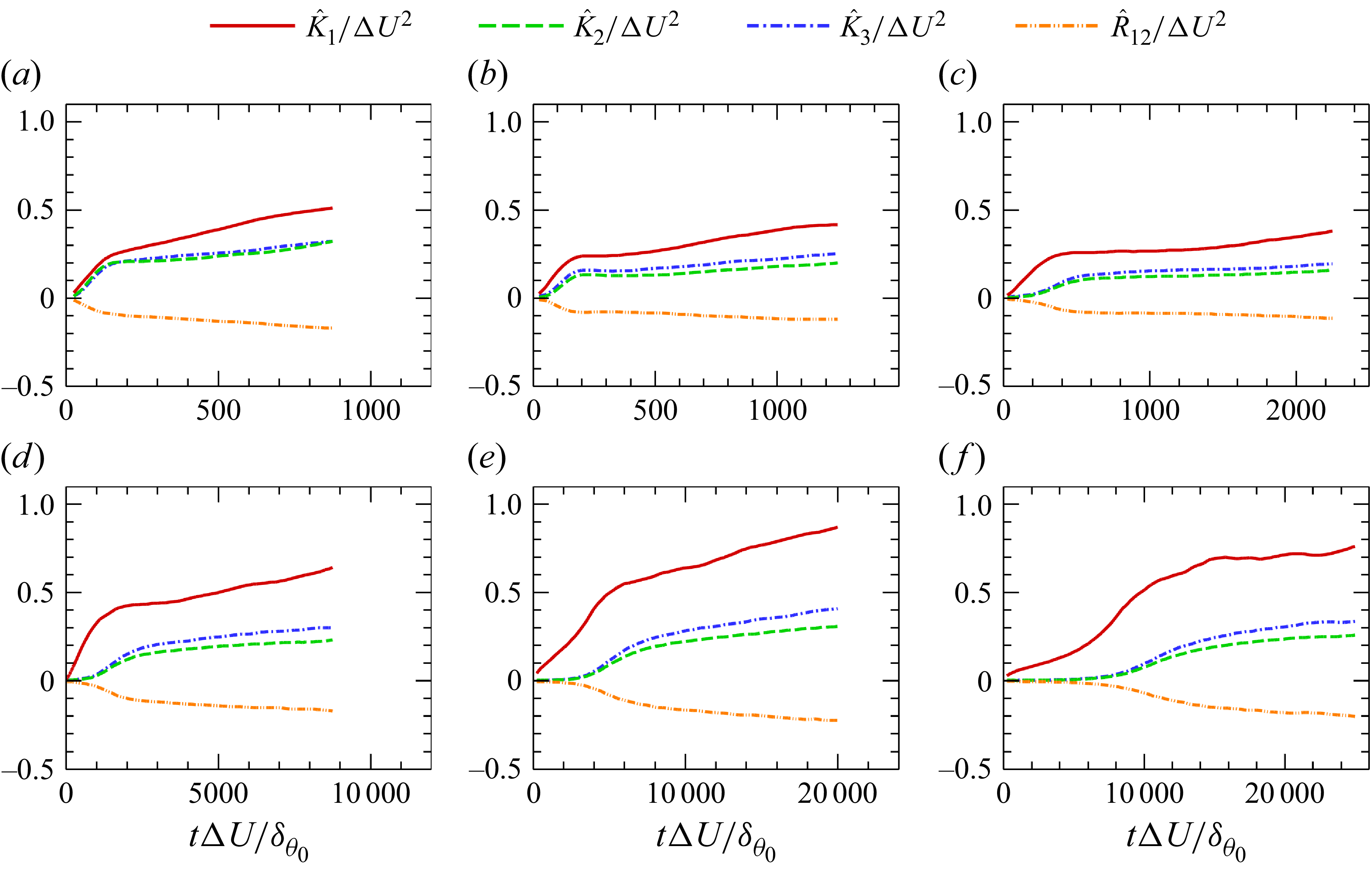
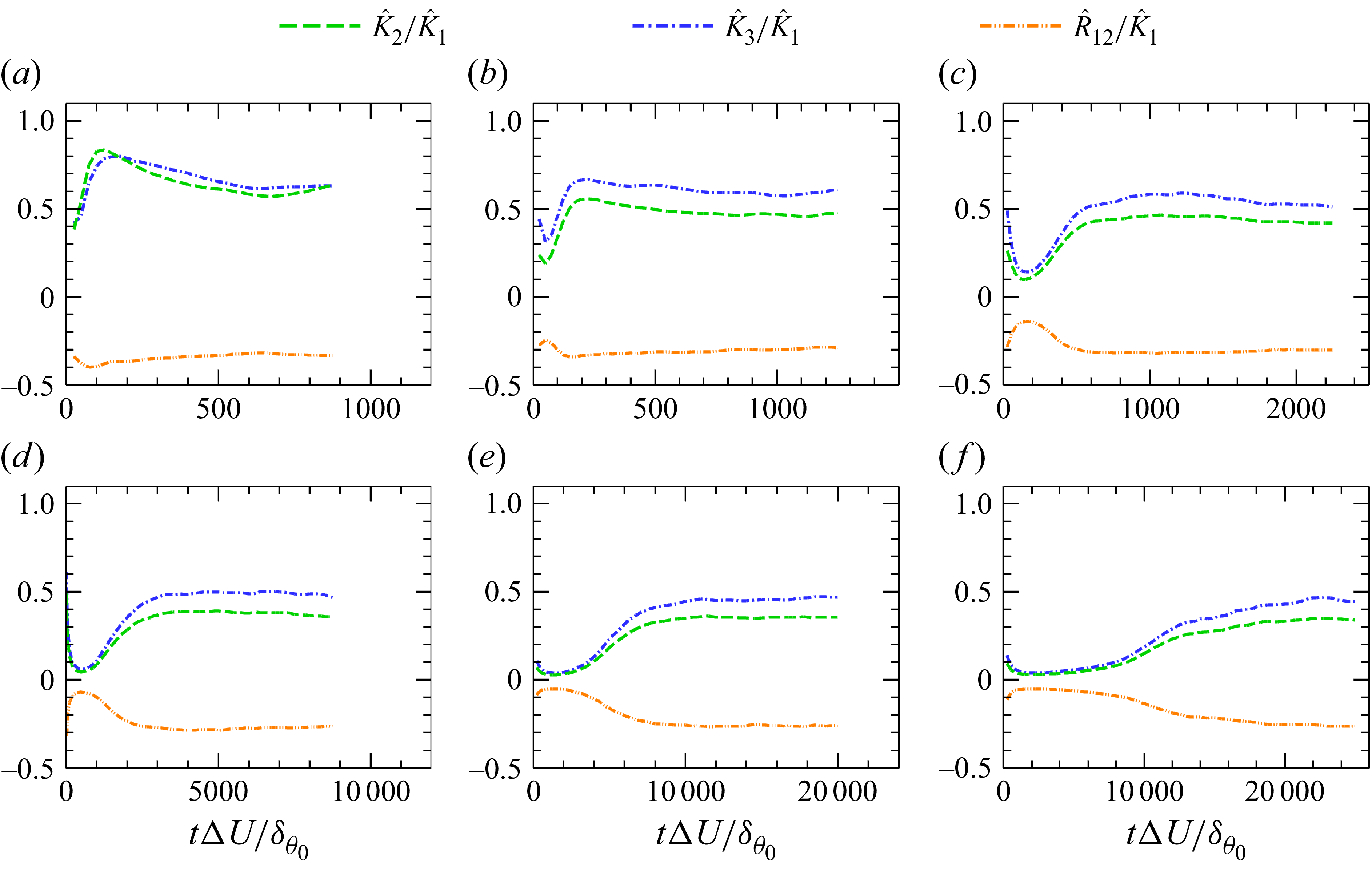
Figure 10 presents the temporal evolution of the total TKE components and the total Reynolds shear stress for different convective Mach numbers. As
 $M_c$
increases, the growth of the vertical and spanwise TKE components becomes increasingly delayed relative to the streamwise component. Under weakly compressible conditions (
 $M_c=0.2$
), all three components grow almost simultaneously. In contrast, at
 $M_c=5.0$
, the growth of the vertical and spanwise components exhibits no noticeable increase until
 $\tau \approx 8000$
. This behaviour demonstrates that compressibility increasingly suppresses the transfer of energy from the streamwise component to the transverse components as
 $M_c$
rises.
Temporal evolution of the total TKE components (
 $ \hat {K_i}/\Delta U^2$
) and the total Reynolds shear stress (
 $ \hat {R}_{12}/\Delta U^2$
) for different convective Mach numbers
 $M_c$
: (a)
 $ M_c=0.2$
, (b)
 $ M_c=0.8$
, (c)
 $ M_c=1.8$
, (d)
 $ M_c=3.0$
, (e)
 $ M_c=4.0$
and (f)
 $ M_c=5.0$
.

Temporal evolution of
 $ \hat {K_2}/\hat {K_1}$
,
 $ \hat {K_3}/\hat {K_1}$
and
 $ \hat {R}_{12}/\hat {K_1}$
for different convective Mach numbers
 $M_c$
: (a)
 $ M_c=0.2$
, (b)
 $ M_c=0.8$
, (c)
 $ M_c=1.8$
, (d)
 $ M_c=3.0$
, (e)
 $ M_c=4.0$
and (f)
 $ M_c=5.0$
.

Figure 11 shows the ratios of the vertical and spanwise TKE components, as well as the Reynolds shear stress, to the streamwise TKE. It can be seen that the anisotropy of TKE increases significantly with increasing Mach number, especially during the transition stage. Once the turbulence becomes fully developed, these ratios attain statistically steady values. At
 $M_c=0.2$
, the vertical and spanwise TKE components are nearly equal, each reaching approximately 60 %–70 % of the streamwise TKE. For
 $M_c \geqslant 0.8$
, the vertical TKE becomes clearly smaller than the spanwise one. As
 $M_c$
increases from 0.8 to 5.0, the ratio
 $ \hat {K_3}/\hat {K_1}$
decreases from about 0.6 to below 0.5, while
 $ \hat {K_2}/\hat {K_1}$
drops from 0.5 to around 0.3. In contrast, the ratio of the total Reynolds shear stress to the streamwise TKE,
 $ \hat {R_{12}}/\hat {K_1}$
, exhibits only a weak dependence on
 $M_c$
, remaining close to 0.3 across all cases. These observations are consistent with the findings of Pantano & Sarkar (Reference Pantano and Sarkar2002). The increase in anisotropy leads to a clear change in the morphology of the large-scale structures. At low Mach numbers, the flow is dominated by spanwise-oriented K–H rollers, characterised by a relatively large contribution of vertical and spanwise TKE. As compressibility increases, the flow progressively transitions to elongated LSSs, accompanied by a pronounced reduction of the vertical and spanwise TKE (Bell & Mehta Reference Bell and Mehta1990; Rogers & Moser Reference Rogers and Moser1994; Balaras, Piomelli & Wallace Reference Balaras, Piomelli and Wallace2001; Pantano & Sarkar Reference Pantano and Sarkar2002; Wang et al. Reference Wang, Wang and Chen2022).
Temporal evolution of
 $ \hat {P}_i/\Delta U^3$
,
 $ \hat {\epsilon }_i/\Delta U^3$
and
 $ \hat {\varPhi }_i/\Delta U^3$
for different convective Mach numbers
 $M_c$
: (a)
 $ M_c=0.2$
, (b)
 $ M_c=0.8$
, (c)
 $ M_c=1.8$
, (d)
 $ M_c=3.0$
, (e)
 $ M_c=4.0$
and (f)
 $ M_c=5.0$
.

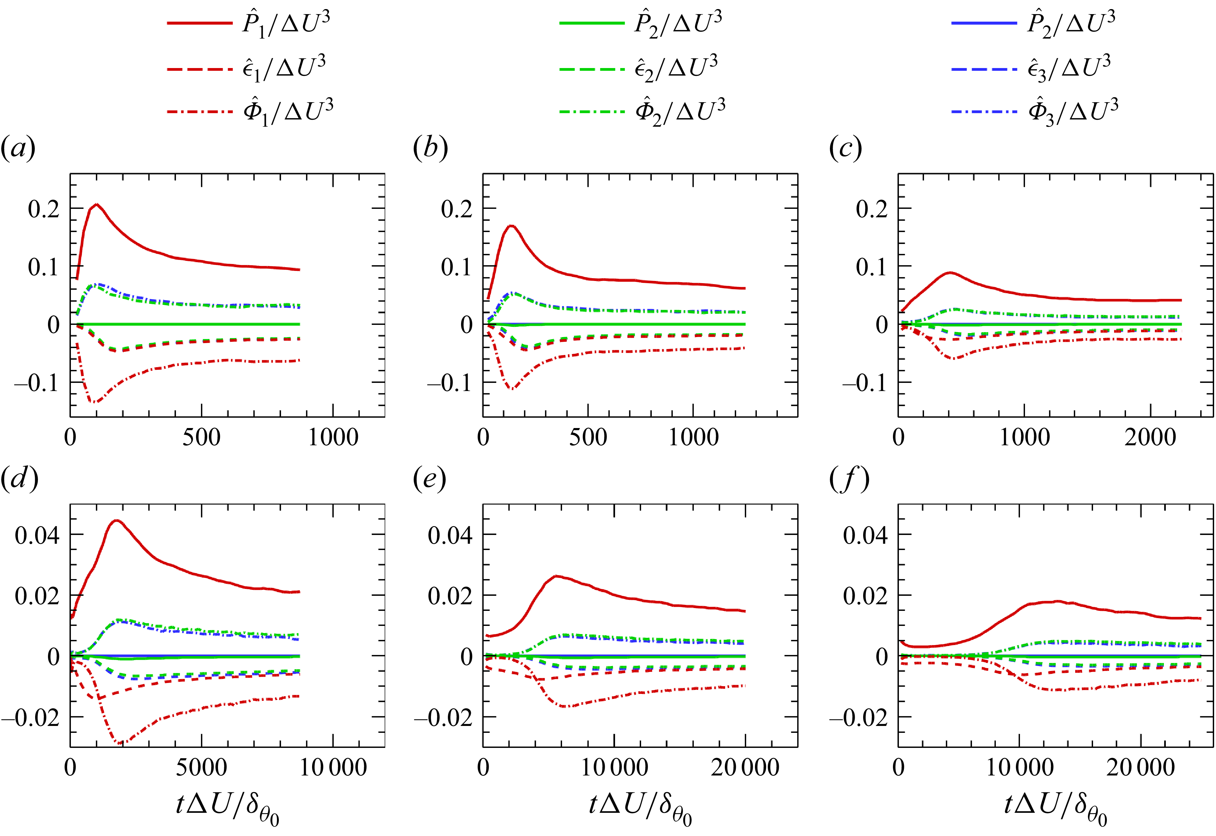
Figure 12 shows the temporal evolution of the integrated TKE transport terms. All terms increase during the transition stage and subsequently decay towards statistically steady levels, consistent with the temporal evolution of the streamwise length scale of the large-scale structures. The effects of compressibility can be summarised as follows. First, the magnitude of all transport terms decreases significantly with increasing
 $M_c$
. At the statistically steady stage, the amplitudes at
 $M_c=5.0$
are about one order of magnitude smaller than those at
 $M_c=0.2$
. Second, the temporal evolution of the transport terms becomes slower at higher
 $M_c$
, with noticeable differences among the individual components. For the dissipation term, the three components nearly collapse for
 $M_c \leqslant 0.8$
, whereas for
 $M_c \geqslant 1.8$
the streamwise component becomes dominant during the transition stage and remains slightly larger in the statistically steady stage. For the pressure–strain redistribution term, its growth rate during the transition stage decreases markedly with increasing
 $M_c$
, and at
 $M_c=5.0$
it remains nearly zero for a long period (
 $\tau \lt 6000$
). Consequently, at higher Mach numbers (
 $M_c \geqslant 1.8$
), there exists a time interval during which the streamwise component of the pressure–strain term becomes smaller than the corresponding dissipation component, and at
 $M_c=5.0$
this imbalance persists until
 $\tau \approx 10\,000$
.
Temporal evolution of
 $ \hat {\epsilon }_i/\hat {P}_1$
and
 $ \hat {\varPhi }_i/\hat {P}_1$
for different convective Mach numbers
 $M_c$
: (a)
 $ M_c=0.2$
, (b)
 $ M_c=0.8$
, (c)
 $ M_c=1.8$
, (d)
 $ M_c=3.0$
, (e)
 $ M_c=4.0$
and (f)
 $ M_c=5.0$
.

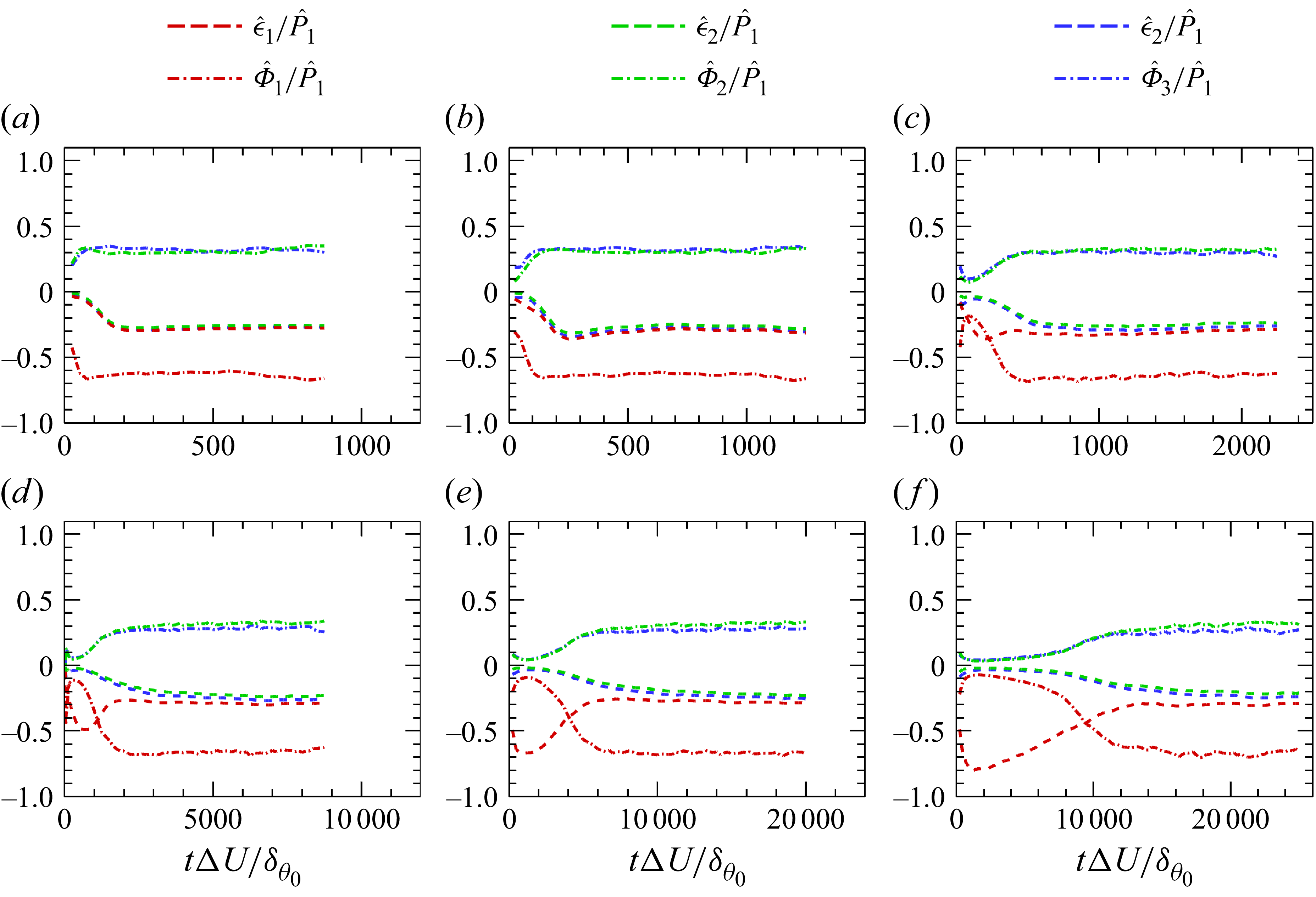
In figure 13, the dissipation and pressure–strain redistribution terms are normalised by the production term. After this normalisation, the peak magnitudes of both dissipation and redistribution become weaker, and a clear statistically steady stage emerges, especially for low to moderate Mach numbers (
 $M_c \leqslant 1.8$
). This behaviour occurs because their temporal variations are similar, and the peak times of the different components are nearly coincident, except for the streamwise component of dissipation.
As discussed in the previous sections, when
 $M_c \geqslant 1.8$
, the streamwise large-scale structures experience a distinct process of initial elongation followed by shortening towards a statistically steady state. Moreover, the duration of this process increases noticeably with
 $M_c$
, providing a valuable opportunity to examine the mechanism governing the evolution of large-scale structures. Therefore, in the following, the case of
 $M_c = 5.0$
is selected as a representative example to analyse the evolution process of the large-scale streamwise structures in detail.
During the stage where the streamwise scale of the large-scale structures
 $l_x$
increases (
 $\tau \lt 5000$
), the streamwise TKE component is dominated by production and dissipation. The dissipation term reaches its peak around
 $\tau \approx 1000$
, attaining approximately 80 % of the production level, which is likely caused by the strong shear across the interface between high- and low-speed large-scale structures. In contrast, the redistribution term grows very slowly, remaining below 10 % of the production term. As a result, the vertical and spanwise TKE components increase only weakly, and the large-scale structures are nearly aligned with the streamwise direction, exhibiting very limited spanwise meandering, as shown in figure 4(a).
In the subsequent stage, where
 $l_x$
decreases (
 $5000 \lt \tau \lt 12\,000$
), the dissipation term decreases approximately linearly, while the redistribution term begins to increase more rapidly. As shown in figure 4(b), small-scale structures start to emerge along the interfaces of the large-scale structures, facilitating the transfer of energy from the streamwise to the vertical and spanwise components. The growth of vertical TKE enhances the production of Reynolds shear stress, which in turn accelerates the growth of the total TKE production. Meanwhile, the increasing spanwise TKE leads to stronger spanwise meandering of the large-scale structures, which eventually suppresses the further growth of the production term.
In the statistically steady stage, all the cases at different convective Mach numbers
 $M_c$
are analysed together, since the dissipation and redistribution terms exhibit little sensitivity to
 $M_c$
. For the streamwise TKE, the dissipation term counteracts about
 $20\,\%$
–
 $30\,\%$
of the production, while the redistribution term offsets approximately
 $60\,\%$
–
 $70\,\%$
. For the vertical and spanwise components, the redistribution term serves as the main energy source, contributing about
 $25\,\%$
–
 $35\,\%$
of the streamwise production, whereas that of the dissipation term is slightly smaller, about
 $20\,\%$
–
 $30\,\%$
. As
 $M_c$
increases, the overlap between the dissipation and redistribution terms becomes less pronounced, indicating that small-scale anisotropy becomes more pronounced. The streamwise dissipation term is the largest among the three components. The redistribution term in the vertical direction exceeds that in the spanwise direction, whereas the dissipation term shows the opposite trend. Since the production in the vertical direction is negative – about
 $5\,\%$
of the streamwise production – and the spanwise production is nearly zero, the vertical TKE remains smaller than the spanwise one. At this stage, the energy exchange among the three velocity components reaches a near-equilibrium state, while the large-scale structures enter a self-sustained regime and their characteristic scales become statistically steady.
4. Conclusion
DNS of compressible turbulent mixing layers have been performed for convective Mach numbers up to
 $M_c = 5.0$
, which is significantly higher than the Mach numbers (typically
 $M_c \lesssim 2.0$
) examined in previous numerical studies. This makes it possible to investigate the effects of compressibility on the evolution, spatial organisation and dynamical balance of elongated LSSs. As the convective Mach number increases, the growth rate of the momentum thickness continues to decrease and shows no indication of saturation. For cases with
 $M_c \geqslant 3.0$
, compressibility markedly slows the development of the mixing layer, making it possible to clearly distinguish the following three stages of LSS evolution:
(i) Growth stage.
-
In this stage, the flow is primarily controlled by the production and dissipation terms of kinetic energy, with the pressure–strain redistribution term being very weak. As a result, streamwise TKE increases rapidly, while spanwise and vertical components remain relatively small. This causes the LSSs to grow rapidly in the streamwise direction. With increasing compressibility, the streamwise scale elongates more dramatically, reaching up to
$30\delta _\omega$
at
$ M_c = 5.0$
. In this stage, the LSSs are well formed, smooth and nearly parallel to the streamwise direction, with minimal spanwise meandering.


(ii) Breakdown stage.
-
As the strength of the LSSs increases, the shear layer at the interfaces between high- and low-speed regions intensifies. This leads to the formation of small-scale structures. The increase in small scales enhances the pressure–strain redistribution, transferring kinetic energy from the streamwise component to the vertical and spanwise components. Vertical TKE rises, triggering a more active turbulent energy transport, while spanwise TKE increases, causing the LSSs to meander and eventually break down, reducing their streamwise length. The spanwise meandering is a key factor in limiting the growth of turbulent energy.
(iii) Self-similar stage.
-
In this stage, the production, pressure–strain redistribution and dissipation terms of kinetic energy reach a equilibrium state and jointly govern the evolution of the flow. The streamwise scale of the large-scale structures stabilises at a constant value, which increases with compressibility.
In contrast, the spanwise scale becomes less sensitive to compressibility and gradually approaches a constant value of
 $0.4\delta _\omega$
over time, though the time to reach this steady state increases with higher Mach numbers. In the self-similar regime, the spatial scale of the LSSs is comparable to that observed in the outer region of wall-bounded turbulence, suggesting a degree of universality in the organisation of large-scale motions across different types of shear turbulence.
With increasing compressibility, the flow becomes increasingly anisotropic. In the near-incompressible regime dominated by K–H rollers, the spanwise and vertical components of the TKE reach up to about 60 % of the streamwise component. As the Mach number increases, the contributions of these two components decrease progressively. When
 $ M_c\geqslant 3.0$
, the vertical TKE drops to less than 35 % of the streamwise value, while the spanwise component falls below 50 %. The reduction of spanwise and vertical TKE indicates weaker cross-stream motions, which in turn stabilises the LSSs and allows their streamwise scale to grow substantially.
Acknowledgements
This work was supported by NSFC Excellence Research Group Program for ‘Multiscale Problems in Nonlinear Mechanics’ (no. 12588201), by the National Natural Science Foundation of China (NSFC grant nos. 12588301, 12272371, 12172161, 12494543 and 12161141017), by the Shenzhen Science and Technology Program (grant nos. SYSPG20241211173725008 and KQTD20180411143441009) and by the Department of Science and Technology of Guangdong Province (grant nos. 2019B21203001, 2020B1212030001 and 2023B1212060001). Additional support was provided by the Innovation Capability Support Program of Shaanxi (no. 2023-CXTD-30) and the Center for Computational Science and Engineering of Southern University of Science and Technology.
Declaration of interests
The authors report no conflict of interest.

 Lx
 Ly
 Lz
 δθ0
 Nx
 Ny
 Nz

 x−y
 Mt
 ρ¯
 ρrms
 T¯
 Trms
 η
 lx
 lz
 y=0
 Mc=3.0
 4.0
 5.0
 Mc

 u′′<0.0
 x−z
 Mc=3.0
 τ=200
 τ=1250
 τ=7500

 u′′<0.0
 x−z
 Mc=4.0
 τ=2000
 τ=6250
 τ=17500

 u′′<0.0
 x−z
 Mc=5.0
 τ=5000
 τ=10000
 τ=22500
 Mc=4.0
 Rxu
 τ=250
 1500
 τ=2000
 7500
 Rzu
 τ=500
 14500
 δω
 lx/δω
 Rth=0.05, 0.1
 lx/δω
 Mc=0.2
 Mc=0.8
 Mc=1.8
 Mc=3.0
 Mc=4.0
 Mc=5.0
 lz/δω
 Rth=0.05, 0.1
 lz/δω
 Mc=0.2
 Mc=0.8
 Mc=1.8
 Mc=3.0
 Mc=4.0
 Mc=5.0
 (lx/δω)max
 Mc
 (lx/δω)self
 (lz/δω)self
 Mc
 (lx/lz)self
 Ki^/ΔU2
 R^12/ΔU2
 Mc
 Mc=0.2
 Mc=0.8
 Mc=1.8
 Mc=3.0
 Mc=4.0
 Mc=5.0
 K2^/K1^
 K3^/K1^
 R^12/K1^
 Mc
 Mc=0.2
 Mc=0.8
 Mc=1.8
 Mc=3.0
 Mc=4.0
 Mc=5.0
 P^i/ΔU3
 ϵ^i/ΔU3
 Φ^i/ΔU3
 Mc
 Mc=0.2
 Mc=0.8
 Mc=1.8
 Mc=3.0
 Mc=4.0
 Mc=5.0
 ϵ^i/P^1
 Φ^i/P^1
 Mc
 Mc=0.2
 Mc=0.8
 Mc=1.8
 Mc=3.0
 Mc=4.0
 Mc=5.0


