





1 Introduction
The development of the optimal designs presented in this article was motivated by research on retest effects in cognitive abilities, which have been a central topic in educational research, psychology, and neuroscience for many years. Retest effects, also known as practice or test effects, denote systematic changes in performance that occur when individuals complete the same or equivalent cognitive ability tests repeatedly under comparable conditions. Several meta-analyses have demonstrated that repeated assessments of core cognitive abilities typically lead to substantial score improvements that follow a nonlinear trajectory characterized by diminishing gains across successive test administrations.
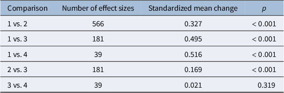
For example, a comprehensive longitudinal multilevel meta-analysis by Scharfen et al. (Reference Scharfen, Peters and Holling2018) examined retest effects across a large number of cognitive ability tests with up to four test administrations. Table 1 summarizes the results aggregated across tests assessing reasoning, memory, processing speed, and divergent thinking, the primary dimensions of intelligence according to the Berlin model of intelligence structure (BIS; Jäger, Reference Jäger1982). As shown in Table 1, statistically significant successive retest effects were observed up to the third test administration. However, in some tests that measure more specific cognitive abilities such as verbal performance or memory, significant score increases were also found between the third and fourth test administrations.
Summary of retest effects reported by Scharfen et al. (Reference Scharfen, Peters and Holling2018)

Table 1 Long description
The table consists of four columns: Comparison, Number of effect sizes, Standardized mean change, and p.
* Row 1: Comparison 1 vs. 2; 566 effect sizes; 0.327 mean change; p less than 0.001.
* Row 2: Comparison 1 vs. 3; 181 effect sizes; 0.495 mean change; p less than 0.001.
* Row 3: Comparison 1 vs. 4; 39 effect sizes; 0.516 mean change; p less than 0.001.
* Row 4: Comparison 2 vs. 3; 181 effect sizes; 0.169 mean change; p less than 0.001.
* Row 5: Comparison 3 vs. 4; 39 effect sizes; 0.021 mean change; p equals 0.319.
Furthermore, the meta-analysis revealed substantial heterogeneity in retest effects across samples. Such individual differences must be taken into account to ensure valid interpretation of test outcomes, particularly when test-takers differ in their prior testing experience.
Longitudinal studies of cognitive abilities are typically time-consuming and resource-intensive. Recruiting participants is often difficult, and dropout rates tend to increase as studies progress, especially when tasks are tedious, cognitively demanding, or insufficiently motivating. From a practical and ethical perspective, it is therefore desirable to minimize the total number of test items administered across all measurement occasions while ensuring sufficient statistical efficiency for estimating the parameters of interest. To address this problem, we develop optimal designs for the longitudinal Rasch Poisson Gamma counts model (RPGCM).
The RPGCM is based on the Rasch Poisson counts model (RPCM), which was originally introduced by Rasch (Reference Rasch1960) for the analysis of count data and is often regarded as one of the earliest item response models (Baghaei & Doebler, Reference Baghaei and Doebler2019). Like the more widely known logistic Rasch model, the RPCM includes both an ability parameter and an item difficulty parameter. Rasch applied this model to oral reading performance, measured by the number of words read and the number of errors, which followed a Poisson distribution. More generally, the model may be applicable to a wide range of ability test data, as three of the four BIS intelligence dimensions, memory, processing speed, and divergent thinking, yield count data.
The original RPCM was specified as a fixed-effects model. Subsequent developments introduced random effects for both person and item parameters. In particular, gamma-distributed person parameters have received considerable attention (e.g., Graßhoff et al., Reference Graßhoff, Holling and Schwabe2020; Jansen & van Duijn, Reference Jansen and van Duijn1992; Owen, Reference Owen1969). As the conjugate prior of the Poisson distribution, the gamma distribution possesses several attractive statistical properties compared with alternative specifications such as the log-normal distribution (Jansen, Reference Jansen1986). In particular, the resulting marginal response distribution is a negative binomial distribution, which naturally accommodates the overdispersion often encountered in count data (e.g., Hung, Reference Hung2012). In some studies, item parameters were also modeled as random effects, for example, by means of a Dirichlet distribution (Jansen, Reference Jansen1997) or a log-normal distribution (Jansen, Reference Jansen1986). A further line of development concerns the introduction of discrimination parameters. Myszkowski and Storme (Reference Myszkowski and Storme2021) extended the RPCM beyond the one-parameter framework by incorporating discrimination effects. However, their approach retained the assumption of equidispersion inherent in the Poisson distribution. This limitation was addressed by Beisemann (Reference Beisemann2022), who proposed a Conway–Maxwell–Poisson (CMP) extension of the RPCM. In addition to item discrimination parameters, the CMP approach permits the modeling of both overdispersion and underdispersion, thereby substantially increasing the flexibility of the model.
The introduction of approaches using finite mixture models and latent classes represents a further extension of the RPCM. For example, van Duijn and Böckenholt (Reference van Duijn and Böckenholt1995) demonstrated that repeated count observations may be explained by transitions between discrete latent classes. Similarly, Verhelst and Kamphuis (Reference Verhelst and Kamphuis2009) argued that speed-test data may require mixture formulations of the RPCM to adequately capture latent heterogeneity.
Another important development, which also does not assume a single continuous latent variable, is the development of multidimensional Poisson count models, which allow for the simultaneous modeling of multiple latent variables and their interrelationships. For example, Wedel et al. (Reference Wedel, Böckenholt and Kamakura2003) proposed multivariate factor-analytic Poisson models. Skrondal and Rabe-Hesketh (Reference Skrondal and Rabe-Hesketh2004) embedded the RPCM and related extensions within the general framework of generalized linear latent and mixed models. This framework provides a unified likelihood-based approach to multilevel, longitudinal, and structural equation models for count data. To date, the most comprehensive multidimensional extension appears to be the multidimensional two-parameter CMP model proposed by Beisemann et al. (Reference Beisemann, Holling and Doebler2025). This framework combines item discrimination parameters with flexible dispersion modeling and thus generalizes both multidimensional IRT models and generalized count models. A particularly innovative feature is the incorporation of rotation and regularization techniques to obtain sparse and interpretable loading structures. As a result, multidimensional count models become substantially more interpretable and consequently more useful for applied psychometric research.
To develop optimal designs for studies analyzing retest effects of cognitive abilities, we begin with a longitudinal version of the RPGCM. This model is particularly suitable when the item parameters are known, for example, when items are drawn from calibrated tests. Moreover, as outlined above, the gamma distribution constitutes an advantageous choice for the ability parameters. In longitudinal settings, the RPGCM must be extended, since dependencies between repeated measurements within individuals have to be taken into account. To this end, we adopt a longitudinal RPGCM based on the established concept of compound symmetry, following Parsamaram et al. (Reference Parsamaram, Holling and Schwabe2026). An analogous framework for the analysis of metric repeated measurements using linear mixed models with multivariate normal random effects was proposed by Freise et al. (Reference Freise, Holling and Schwabe2023). Should more sophisticated Poisson count models be required for the analysis of retest effects in cognitive abilities, the development of corresponding optimal designs remains an important topic for future research.
The remainder of the article is structured as follows. Section 2 describes the longitudinal RPGCM and outlines parameter estimation using maximum quasi-likelihood. Section 3 derives A-optimal designs for estimating mean abilities and common functions thereof under an unstructured mean model. Furthermore, these designs are illustrated using some growth patterns with four measurement occasions. In the final section, we briefly discuss the differences between the A-optimal designs derived in the present study and the corresponding D-optimal designs developed by Parsamaram et al. (Reference Parsamaram, Holling and Schwabe2026). The article concludes with a summary and suggestions for future research.
2 Longitudinal Rasch Poisson Gamma counts model
This section outlines the longitudinal RPGCM and the estimation of its parameters. A more detailed technical description can be found in Parsamaram et al. (Reference Parsamaram, Holling and Schwabe2026).
2.1 Model specification
Let
$Y_{ijk}$
 denote the response of test person
$i$
 to item
$k$
 administered at the
$j$
 th measurement occasion taking place at time
$t_j$
 . The response is assumed to follow a Poisson distribution with mean
$\theta _{ij}\sigma _{jk}$
 , where
$\theta _{ij}$
 denotes the ability of person
$i$
 at time
$t_j$
 ,
$i = 1, \ldots , N$
 ,
$j = 1, \ldots , J$
 , and
$\sigma _{jk}$
 denotes the easiness of item
$k$
 administered at time
$t_j$
 ,
$k = 1, \ldots , n_j$
 .
The subjects are assumed to receive the same items with easiness
$\sigma _{jk}$
 and, in particular, the same total number
$n_j$
 at occasion
$j$
 ,
$\sum _{j=1}^{J} n_j = n$
 , each. Furthermore, the item easiness parameters
$\sigma _{jk}$
 are assumed to be known, which does not constitute a restriction when calibrated tests are employed, and the mean item easiness
$\bar {\sigma } = \frac {1}{n}\sum _{j=1}^{J}\sum _{k=1}^{n_j}\sigma _{jk}$
 is fixed. This condition is trivially satisfied if the same item parameters are used across time points. When automatically generated, rule-based items are administered, this assumption typically does not pose practical problems.
The primary objective of the analysis is the estimation of the development of ability over time, represented by a common mean learning curve
$\theta (t)$
 evaluated at
$t_1, \ldots , t_J$
 . Optimal designs allow
$\theta (t)$
 to be estimated with maximal precision as a function of the allocation of items across measurement occasions, that is, the proportions
$n_j / n$
 and the items
$\sigma _{jk}$
 ,
$k = 1, \ldots , n_j$
 . In empirical applications, the same number
$n_j = n / J$
 of items is often presented with common mean item easiness
$\bar {\sigma }_j = \frac {1}{n_j}\sum _{k=1}^{n_j}\sigma _{jk}$
 at each measurement occasion, that is,
$n_j = n / J$
 and
$\bar {\sigma }_j = \bar {\sigma }$
 . This practice raises the question of whether such a design is efficient or whether alternative allocations can reduce the total number of items required without compromising statistical accuracy.
Abilities
$\theta _{ij}$
 are modeled as random effects. Specifically,
$\theta _{ij}$
 is expressed as a realization of

where
$\Lambda _{ij}$
 is a gamma-distributed latent variable capturing individual deviations from the mean trajectory
$\theta (t)$
 .
To specify a longitudinal RPGCM based on compound symmetry, analogous to linear mixed models with multivariate normal random effects, a permanent person effect and time-specific person effects are introduced. Accordingly, the latent variable
$\Lambda _{ij}$
 is decomposed as

where the time-specific effects
$\Gamma _{i1}, \ldots , \Gamma _{iJ}$
 are assumed to be independently and identically distributed as
$\Gamma (\alpha , \tau )$
 , the permanent person effect
$\Gamma _{i0} \sim \Gamma (\alpha _0, \tau )$
 shares the same scale parameter
$\tau $
 , and all components are mutually independent.
Under these assumptions,
$\Lambda _{ij} \sim \Gamma (\alpha _0 + \alpha , \tau )$
 , and the vector
$\boldsymbol {\Lambda }_i = (\Lambda _{i1}, \ldots , \Lambda _{iJ})^\top $
 follows a multivariate gamma distribution with correlated components induced by the permanent person effect.
By standardizing the latent effects by
$\tau = 1 / (\alpha _0 + \alpha )$
 such that
$\mathrm {E}(\Lambda _{ij}) = 1$
 , the marginal mean of the responses is given by

Thus, the growth curve
$\theta (t)$
 represents the marginal mean ability, satisfying
$\mathrm {E}(\Theta _{ij}) = \theta (t_j)$
 .
Furthermore,
$\mathrm {Var}(\Lambda _{ij}) = \tau $
 and
$\mathrm {Cov}(\Lambda _{ij}, \Lambda _{ij'}) = \rho \tau $
 , where
$\rho = \alpha _0 \tau $
 denotes the intraclass correlation coefficient. Consequently,

To model the mean structure, we adopt an unstructured one-way ANOVA-type specification
$\theta (t_j) = \theta _j$
 embedded in a generalized linear mixed model with a log link,

with vector
$\boldsymbol {\theta } = (\theta _1, \ldots , \theta _J)$
 of mean abilities over time.
In the model outlined above, the latent variables
$\Gamma _{ij}$
 are assumed to be identically distributed across measurement occasions. Consequently, the variances of the ability parameters
$\Theta _{ij}$
 remain constant over time. For many studies investigating retest effects in cognitive abilities, this assumption appears plausible. We inspected the studies included in the meta-analysis by Scharfen et al. (Reference Scharfen, Peters and Holling2018) and found that the variances of the observed test scores were generally stable across repeated measurement occasions. However, gains in ability may not be strictly additive. For example, individuals with higher initial abilities may exhibit different growth trajectories than individuals with lower initial abilities. In such situations, the assumption of constant variance may be violated. To accommodate this possibility, we extend the model by allowing the latent variables to follow occasion-specific gamma distributions,
$ \Gamma _{ij} \sim \Gamma (\alpha _j,\tau ), j = 1,\ldots ,J$
 , thereby permitting the variances of the ability parameters to vary over time. The extended model, together with the corresponding optimal designs, is presented in the Appendix. It should be noted, however, that the resulting A-optimal designs depend on the variance parameters of the random effects, whereas the designs obtained under the assumption of identically distributed
$\Gamma _{ij}$
 do not. Thus, they require substantially more prior information, which may be difficult to obtain in practical applications.
2.2 Parameter estimation
In the generalized linear mixed model setup, the focus is on estimating the parameter vector
$\boldsymbol {\beta } = (\beta _1, \ldots , \beta _J)^\top $
 . Even if the parameters
$\tau $
 and
$\rho $
 are assumed to be known, the likelihood involves integrals which are analytically difficult to handle. Consequently, we employ maximum quasi-likelihood estimation (Wedderburn, Reference Wedderburn1974), which relies only on the first- and second-order marginal moments of the response vector.
The maximum quasi-likelihood estimator
$\hat {\boldsymbol {\beta }}_{\mathrm {MQL}}$
 is defined as the solution to

where
$\boldsymbol {\mu }_i = \mathrm {E}(\mathbf {Y}_i)$
 ,
$\mathbf {V}_i = \mathrm {Cov}(\mathbf {Y}_i)$
 , and
$\mathbf {D}_i = \partial \boldsymbol {\mu }_i / \partial \boldsymbol {\beta }^\top $
 . The explicit expressions for these terms are provided in the Appendix.
The quasi-information matrix is given by

Similar to the situation in maximum likelihood estimation, the asymptotic covariance matrix of the maximum quasi-likelihood estimator
$\hat {\boldsymbol {\beta }}_{\mathrm {MQL}}$
 is proportional to the inverse
$\mathbf {M}_{\mathrm {Q}}^{-1}$
 of the quasi-information matrix.
As shown in Theorem 4.2 of Parsamaram et al. (Reference Parsamaram, Holling and Schwabe2026), the quasi-information simplifies, under a saturated mean model and identical test conditions across individuals, to

In the fixed-effects RPCM, the maximum quasi-likelihood estimator coincides with the common maximum likelihood estimator, and the likelihood-based Fisher information for
$\boldsymbol {\beta }$
 is obtained by formally setting
$\tau = 0$
 in the quasi-information.
3 A-optimal design
Parsamaram et al. (Reference Parsamaram, Holling and Schwabe2026) developed locally D-optimal designs for estimating mean abilities in this model. According to their results, the D-optimal designs, which minimize the volume of the confidence ellipsoid of the parameters, require not only the specification of the parameter vector of interest,
$\boldsymbol {\theta }$
 , but also prior knowledge of the variance
$\tau $
 and the correlation
$\rho $
 . Such information, however, is rarely available in practice. In contrast, A-optimal designs, which minimize the sum of the variances of the parameter estimators or specified functions thereof, rely on substantially weaker assumptions and are therefore better suited to practical applications. We will discuss this topic in more detail in the fifth section.
The standardized (per response) quasi-information matrix is

where
$\xi = (w_1, \ldots , w_J)$
 denotes the vector of proportions
$w_j = \sum _{k=1}^{n_j}\sigma _{jk} / \sum _{j=1}^{J}\sum _{k=1}^{n_j}\sigma _{jk}$
 of item easiness allocated to the measurement occasions
$j = 1, \ldots , J$
 ,
$\sum _{j=1}^{J} w_j = 1$
 .
The vector
$\xi $
 of proportions of easiness constitutes the test design and can be chosen to optimize certain characteristics of the estimation. These proportions of easiness can be interpreted as follows: When all items have the same easiness parameters
$\sigma _{jk} = \bar {\sigma }= \frac {1}{n} \sum _{j=1}^J \sum _{k=1}^{n_j} \sigma _{jk}$
 , then
$w_j = n_j / n$
 is the proportion of items presented at occasion
$j$
 . Alternatively, when the same number
$n_j = n / J$
 of items is presented at each occasion, then
$w_j = \frac {1}{J \bar {\sigma }}\bar {\sigma }_j$
 is proportional to the mean easiness
$\bar {\sigma }_j = \frac {1}{n_j}\sum _{k=1}^{n_j}\sigma _{jk}$
 of items to be administered at occasion
$j$
 .
Note that, in the unstructured mean model, the proportions
$w_j$
 are only involved in the first term in the representation of the quasi-information. In particular, the asymptotic covariance matrix of
$\hat {\boldsymbol {\beta }}$
 equals
$c_1 \mathrm {diag}(1/(\theta _j w_j)) + \mathbf {C}_2$
 for some generic constant terms
$c_1> 0$
 and
$\mathbf {C}_2$
 . This explains why the A-optimal weights neither depend on the variance parameters
$\tau $
 and
$\rho $
 nor on
$\bar {\sigma }$
 and
$n$
 .
We derive A-optimal designs for the most relevant parameters of the unstructured longitudinal RPGCM. We begin with the basic parameter vector
$\boldsymbol {\beta }$
 of the unstructured mean model and subsequently develop A-optimal designs for the mean ability vector
$\boldsymbol {\theta } = (\theta _1, \ldots , \theta _J)$
 as well as for the square-root-transformed mean abilities
$\boldsymbol {d} = (d_1, \ldots , d_J)$
 ,
$d_j = \sqrt {\theta _j}$
 .
In many applications, hypotheses are formulated in terms of contrasts rather than absolute parameter values. Accordingly, we also derive A-optimal designs for commonly used contrasts, including differences relative to a baseline (e.g.,
$\theta _j - \theta _1$
 ,
$j = 2, \ldots , J$
 ) and successive differences (e.g.,
$\theta _j - \theta _{j-1}$
 ,
$j = 2, \ldots , J$
 ).
All A-optimality criteria considered in the following can be reduced to the minimization of an objective function of the form

in the proportions of easiness
$w_j$
 allocated to measurement occasion
$j$
 . Minimization of this function yields the optimal weights

This general result considerably simplifies the derivation of the optimal designs presented below.
As an illustration, consider A-optimal designs for the parameters
$\beta _j = \log (\theta _j)$
 ,
$j = 1, \ldots , J$
 . In this case, the trace of the asymptotic covariance matrix has to be minimized. This is equivalent to minimizing

Setting
$h_j = 1/\theta _j$
 immediately yields the A-optimal weights

for estimating the parameters
$\boldsymbol {\beta } = (\beta _1, \ldots , \beta _J)$
 .
3.1 A-optimal designs for
$\boldsymbol{\beta }$


For contrasts relative to the baseline,
$\beta _j - \beta _1$
 ,
$j = 2, \ldots , J$
 , the objective function

has to be minimized, and for successive differences,
$\beta _2 - \beta _1, \ldots , \beta _J - \beta _{J-1}$
 , the objective function

has to be minimized. The resulting A-optimal weights for parameters and contrasts of
$\boldsymbol {\beta }$
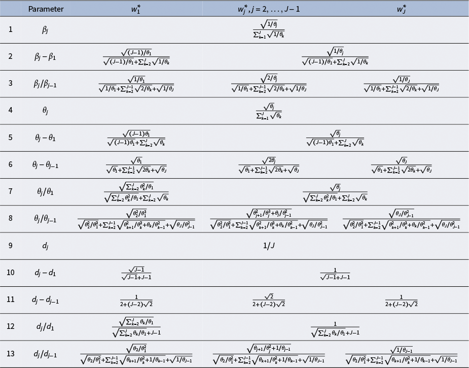
 are listed in lines 1–3 of Table 2.
A-optimal weights for parameters and contrasts

Table 2 Long description
The table contains 13 numbered rows.
Row 1: Parameter beta sub j. Weight for all columns is the square root of 1 over theta sub j all over the summation from k equals 1 to J of the square root of 1 over theta sub k.
Row 2: Contrast beta sub j minus beta sub 1. Weight for w sub 1 superstar is the square root of J minus 1 over theta sub 1 all over the square root of J minus 1 over theta sub 1 plus the summation from k equals 2 to J of the square root of 1 over theta sub k. Weight for other columns is the square root of 1 over theta sub j all over the same denominator.
Row 3: Contrast beta sub j over beta sub j minus 1. Weight for w sub 1 super star is the square root of 1 over theta sub 1 all over a denominator D. Weight for w sub j super star is the square root of 2 over theta sub j all over D. Weight for w sub J super star is the square root of 1 over theta sub J all over D. D equals the square root of 1 over theta sub 1 plus the summation from k equals 2 to J minus 1 of the square root of 2 over theta sub k plus the square root of 1 over theta sub J.
Row 4: Parameter theta sub j. Weight for all columns is the square root of theta sub j all over the summation from k equals 1 to J of the square root of theta sub k.
Row 5: Contrast theta sub j minus theta sub 1. Weight for w sub 1 super star is the square root of J minus 1 times theta sub 1 all over the square root of J minus 1 times theta sub 1 plus the summation from k equals 2 to J of the square root of theta sub k. Weight for other columns is the square root of theta sub j all over the same denominator.
Row 6: Contrast theta sub j minus theta sub j minus 1. Weight for w sub 1 super star is the square root of theta sub 1 all over a denominator D sub 2. Weight for w sub j super star is the square root of 2 times theta sub j all over D sub 2. Weight for w sub J super star is the square root of theta sub J all over D sub 2. D sub 2 equals the square root of theta sub 1 plus the summation from k equals 2 to J minus 1 of the square root of 2 times theta sub k plus the square root of theta sub J.
Row 7: Contrast theta sub j over theta sub 1. Weight for w sub 1 super star is the square root of the summation from k equals 2 to J of theta sub k squared over theta sub 1 all over a denominator D sub 3. Weight for other columns is the square root of theta sub j all over D sub 3. D sub 3 equals the square root of the summation from k equals 2 to J of theta sub k squared over theta sub 1 plus the summation from k equals 2 to J of the square root of theta sub k.
Row 8: Contrast theta sub j over theta sub j minus 1. Weights involve complex square roots of theta ratios. Weight for w sub 1 super star is the square root of theta sub 2 squared over theta sub 1 cubed all over a summation denominator.
Row 9: Parameter d sub j. Weight for all columns is 1 over J.
Row 10: Contrast d sub j minus d sub 1. Weight for w sub 1 super star is the square root of J minus 1 all over the square root of J minus 1 plus J minus 1. Weight for other columns is 1 all over the square root of J minus 1 plus J minus 1.
Row 11: Contrast d sub j minus d sub j minus 1. Weights for w sub 1 super star and w sub J super star are 1 over 2 plus J minus 2 times the square root of 2. Weight for w sub j super star is the square root of 2 over 2 plus J minus 2 times the square root of 2.
Row 12: Contrast d sub j over d sub 1. Weight for w sub 1 super star is the square root of the summation from k equals 2 to J of theta sub k over theta sub 1 all over the square root of the same summation plus J minus 1. Weight for other columns is 1 over the same denominator.
Row 13: Contrast d sub j over d sub j minus 1. Weights involve square roots of theta sub j plus 1 over theta sub j squared plus 1 over theta sub j minus 1.
3.2 A-optimal designs for
$\boldsymbol{\theta }$

In applications of longitudinal Poisson models, the primary parameter of interest is often the trajectory
$\theta $
 . In repeated testing, this may correspond, for example, to the expected number of correctly processed stimuli, in epidemiology to the expected number of rare disease cases, and in criminology to the expected number of aggressive acts.
For estimation of
$\boldsymbol {\theta }$
 , the plug-in estimators
$\hat {\theta }_j = \exp (\hat {\beta }_j)$
 may be used. By the
$\delta $
 -method, the asymptotic covariance matrix of
$\hat {\boldsymbol {\theta }}$
 equals
$c_1 \mathrm {diag}(\theta _j / w_j) + \mathbf {C}_2$
 . Again, applying the general objective function, the following A-optimal designs for
$\boldsymbol {\theta }$
 can be derived.
For mean abilities
$\theta _j$
 ,
$j = 1, \ldots , J$
 , the objective function is

For baseline differences
$\theta _j - \theta _1$
 ,
$j = 2, \ldots , J$
 , the objective function is

For successive differences
$\theta _2 - \theta _1, \ldots , \theta _J - \theta _{J-1}$
 , the objective function is

The corresponding A-optimal weights are given in lines 4–6 of Table 2.
Ratios of expected values are often more stable and interpretable than differences. Again, plug-in estimators can be used and the asymptotic covariance is obtained by the
$\delta $
 -method. For ratios relative to the baseline,
$\theta _j/\theta _1$
 ,
$j = 2, \ldots , J$
 , the objective function is given by

and for successive ratios, it is

The A-optimal weights are in lines 7 and 8 of Table 2.
3.3 A-optimal designs for
$\mathbf{\textit{d}} = \boldsymbol{\sqrt {{\theta }}}$

Poisson variables with large expected values are well approximated by a normal distribution after square root transformation,
$d_j = \sqrt {\theta _j}$
 , with
$\mathrm {E}(\hat {d}_j) \approx \sqrt {\theta _j}$
 and
$\mathrm {Var}(\hat {d}_j) \approx 1/4$
 . Even for smaller values of
$\theta _j$
 , this variance-stabilizing transformation substantially reduces heteroscedasticity.
Applying the
$\delta $
 -method once more, the asymptotic covariance matrix of the plug-in estimator
$\hat {\boldsymbol {d}} = (\hat {d}_1, \ldots , \hat {d}_J)$
 reduces to
$c_1 \mathrm {diag}(1/w_j) + \mathbf {C}_2$
 . Ignoring the constant terms, the resulting covariance structure is identical to that in a one-way ANOVA. Consequently, designs that are A-optimal in the one-way layout are also A-optimal for
$\boldsymbol {d}$
 and related linear contrasts (see lines 9–11 in Table 2). In particular, for
$\boldsymbol {d}$
 itself, the optimal design is uniform on the measurement occasions, that is,
$w^\ast_{j} = 1/J$
 ,
$j = 1, \ldots , J$
 . For ratios of
$\boldsymbol {d}$
 , A-optimal designs are given in Table 2, lines 12 and 13.
3.4 Numerical results
All A-optimal designs for
$\boldsymbol {\beta }$
 ,
$\boldsymbol {\theta }$
 , and their contrasts are locally optimal designs. They depend on the relative change in the mean trajectory between measurement occasions, but not on the overall mean. The latter is in accordance with the property that the combination of ability and easiness may be scaled at will. For
$\boldsymbol {d}$
 and the corresponding difference contrasts, however, the optimal designs are independent of the expected values and, hence, globally optimal for all parameter values. They are functions of the number
$J$
 of measurement occasions only, which substantially simplifies experimental planning.
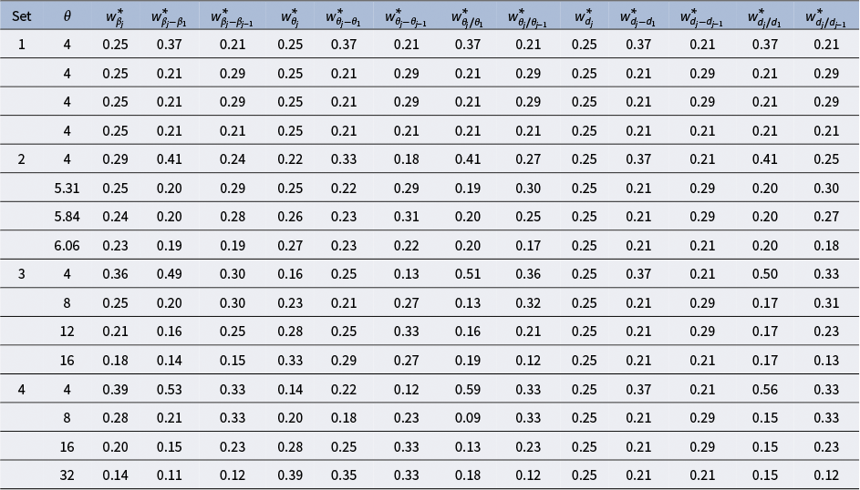
Table 3 illustrates the derived A-optimal designs for four example growth patterns, each with
$J = 4$
 repeated measurements and a baseline with a mean of 4. The first example corresponds to a constant value for the growth curve, which may be considered as a null hypothesis setup of no retest effects. The second example exhibits growth increments motivated by the meta-analysis of retest effects reported by Scharfen et al. (Reference Scharfen, Peters and Holling2018). The third example represents a linear increase in expected values, whereas the fourth example follows an exponential growth curve, as commonly observed in other application domains such as epidemiology.
The results demonstrate once again that A-optimal designs for square-root-transformed parameters and their differences are independent of the actual expected values. In general, a uniform allocation of items across measurement occasions is suboptimal and can lead to a loss of efficiency, in particular, when a baseline measurement serves as a reference. This topic will be analyzed in more detail in the next section.
It should be noted that alternative expected values, growth rates, or numbers of measurement occasions may yield different A-optimal designs. However, the corresponding optimal weights can always be obtained directly from the closed-form expressions derived above.
A-optimal weights for four sets of growth patterns with four measurement occasions each

Table 3 Long description
The table is organized into 15 columns. The first column identifies the Set (1 through 4). The subsequent columns represent mathematical parameters and weights: theta, w super star beta sub j, w super star beta sub j minus beta sub 1, w super star beta sub j minus beta sub j minus 1, w super star theta sub j, w super star theta sub j minus theta sub 1, w super star theta sub j minus theta sub j minus 1, w super star theta sub j over theta sub 1, w super star theta sub j over theta sub j minus 1, w super star d sub j, w super star d sub j minus d sub 1, w super star d sub j minus d sub j minus 1, w super star d sub j over d sub 1, and w super star d sub j over d sub j minus 1.
* Set 1: All theta values are 4. Weights for w super star beta sub j and w super star theta sub j are constant at 0.25. Other weights alternate between 0.37, 0.21, and 0.29.
* Set 2: Theta values increase from 4 to 6.06. Weights for w super star beta sub j decrease from 0.29 to 0.23.
* Set 3: Theta values increase linearly (4, 8, 12, 16). Weights for w super star beta sub j decrease from 0.36 to 0.18. Weights for w super star theta sub j increase from 0.16 to 0.33.
* Set 4: Theta values increase exponentially (4, 8, 16, 32). Weights for w super star beta sub j decrease from 0.39 to 0.14. Weights for w super star theta sub j increase from 0.14 to 0.39. Weights for w super star d sub j remain constant at 0.25 across all sets.
4 A-efficiency
In practice, experimenters frequently employ a uniform allocation of observations across measurement occasions, either for convenience or due to limited prior knowledge about expected values. The previously derived A-optimal designs for the parameter vectors
$\boldsymbol {\beta }$
 ,
$\boldsymbol {\theta }$
 , and
$\boldsymbol {d}=\sqrt {\boldsymbol {\theta }}$
 provide a minimal estimator variance. In this section, we analyze the gain of these optimal designs compared to uniform designs
$\xi _{\mathrm {uniform}} = (1/J, \ldots , 1/J)$
 . Commonly used uniform designs allocate an equal proportion of observations with equal mean easiness to each measurement occasion. Specifically, we consider the A-efficiency of the uniform design compared to the previously obtained A-optimal designs for the parameters
$\boldsymbol {\beta }$
 ,
$\boldsymbol {\theta }$
 , and
$\boldsymbol {d}$
 as well as the contrasts thereof presented in Table 2.
The efficiency, which will be considered here, is defined by

for the uniform design
$\xi _{\mathrm {uniform}}$
 , where
$\boldsymbol {\delta }$
 stands for the parameter vector of interest and
$\xi _{\boldsymbol {\delta }}^\ast$
 is the corresponding A-optimal design.
The A-efficiency ranges between 0 and 1 and quantifies the amount of within-test-person information of the uniform design compared to the A-optimal design. Based on the efficiency, the corresponding A-deficiency can be computed as
$\mathrm {Def}_A(\xi _{\mathrm {uniform}};\boldsymbol {\delta }) = \mathrm {Eff}_A(\xi _{\mathrm {uniform}};\boldsymbol {\delta })^{-1} - 1$
 , which represents the proportional increase in the total number
$n$
 of items required when using design
$\xi _{\mathrm {uniform}}$
 instead of the A-optimal design
$\xi _{\boldsymbol {\delta }}^\ast$
 to achieve the same estimation precision while keeping the mean easiness
$\bar {\sigma }$
 fixed. In the case of the fixed-effects RPCM, the above A-deficiency may be interpreted likewise as the proportional increase in the number
$N$
 of test persons required when the design
$\xi _{\mathrm {uniform}}$
 is used instead of the A-optimal design
$\xi _{\boldsymbol {\delta }}^\ast$
 to obtain the same value for the trace of the covariance matrix while the total easiness
$n \bar {\sigma }$
 per test person is kept fixed.
For the four data examples introduced in Table 3, we compute the A-efficiency of the uniform design relative to the A-optimal design for the parameters
$\boldsymbol {\theta }$
 and
$d$
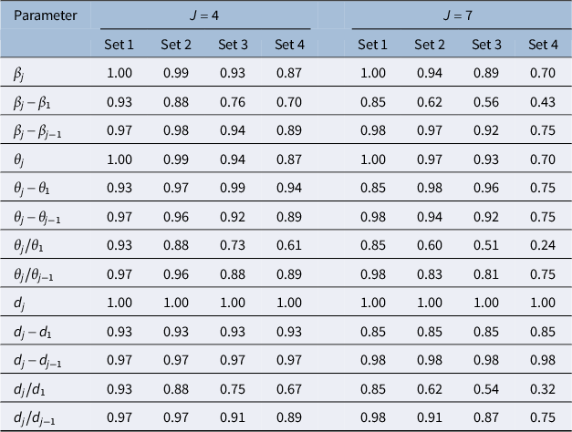
 , as well as for the contrasts considered above. The results are summarized in Table 4 (left). Furthermore, we compute the A-efficiency for another example of four sets of analogous growth patterns, but each with seven measurement occasions. The first set of
$\boldsymbol {\theta }$
 values is constant
$4$
 , the second consists of (4, 8, 11, 13, 14, 14.5, 14.75), the third of (4, 8, 12, 16, 20, 24, 28), and the fourth of (4, 8, 16, 32, 64, 128, 256); see Table 4 (right).
A-efficiency of the uniform design relative to the A-optimal design for the four sets of growth patterns with four measurement occasions as outlined in Table 3 (left) and with seven measurement occasions as outlined in the text (right)

Table 4 Long description
The table is organized by Parameter in the first column, followed by two main sections: J equals 4 (Sets 1 to 4) and J equals 7 (Sets 1 to 4).
Row 1: beta sub j. J equals 4: 1.00, 0.99, 0.93, 0.87. J equals 7: 1.00, 0.94, 0.89, 0.70.
Row 2: beta sub j minus beta sub 1. J equals 4: 0.93, 0.88, 0.76, 0.70. J equals 7: 0.85, 0.62, 0.56, 0.43.
Row 3: beta sub j minus beta sub j minus 1. J equals 4: 0.97, 0.98, 0.94, 0.89. J equals 7: 0.98, 0.97, 0.92, 0.75.
Row 4: theta sub j. J equals 4: 1.00, 0.99, 0.94, 0.87. J equals 7: 1.00, 0.97, 0.93, 0.70.
Row 5: theta sub j minus theta sub 1. J equals 4: 0.93, 0.97, 0.99, 0.94. J equals 7: 0.85, 0.98, 0.96, 0.75.
Row 6: theta sub j minus theta sub j minus 1. J equals 4: 0.97, 0.96, 0.92, 0.89. J equals 7: 0.98, 0.94, 0.92, 0.75.
Row 7: theta sub j over theta sub 1. J equals 4: 0.93, 0.88, 0.73, 0.61. J equals 7: 0.85, 0.60, 0.51, 0.24.
Row 8: theta sub j over theta sub j minus 1. J equals 4: 0.97, 0.96, 0.88, 0.89. J equals 7: 0.98, 0.83, 0.81, 0.75.
Row 9: d sub j. J equals 4: 1.00, 1.00, 1.00, 1.00. J equals 7: 1.00, 1.00, 1.00, 1.00.
Row 10: d sub j minus d sub 1. J equals 4: 0.93, 0.93, 0.93, 0.93. J equals 7: 0.85, 0.85, 0.85, 0.85.
Row 11: d sub j minus d sub j minus 1. J equals 4: 0.97, 0.97, 0.97, 0.97. J equals 7: 0.98, 0.98, 0.98, 0.98.
Row 12: d sub j over d sub 1. J equals 4: 0.93, 0.88, 0.75, 0.67. J equals 7: 0.85, 0.62, 0.54, 0.32.
Row 13: d sub j over d sub j minus 1. J equals 4: 0.97, 0.97, 0.91, 0.89. J equals 7: 0.98, 0.91, 0.87, 0.75.
The results indicate that a uniform allocation of observations is generally suboptimal. A-optimal designs lead to reductions in variance, although these gains are small in several of the examples considered. In such situations, practitioners may rely on uniform designs with only minor loss in efficiency. However, substantially larger reductions are observed for parameters representing contrasts with respect to a reference category. For such contrasts, which are frequently of practical interest, A-optimal designs should therefore be preferred. For any specific situation arising in an empirical study, the formulas presented above allow the derivation of A-optimal designs and the corresponding A-efficiency.
Overall, these findings highlight the practical relevance of A-optimal design strategies for longitudinal and experimental studies when contrasts relative to a reference category are of primary interest.
5 D-optimal versus A-optimal designs for the longitudinal RPGCM
Recently, Parsamaram et al. (Reference Parsamaram, Holling and Schwabe2026) developed locally D-optimal designs for estimating mean abilities in the RPGCM under compound symmetry of the covariance matrix of the random effects. This work motivated us to derive A-optimal rather than D-optimal designs here, although the latter constitute the most prominent class of optimal designs. While a D-optimal design maximizes the determinant of the Fisher information matrix and thereby minimizes the volume of the asymptotic confidence ellipsoid for the parameter vector, an A-optimal design minimizes the trace of the inverse information matrix, this means that it minimizes the average asymptotic variance of the parameter estimates. A major reason for the predominance of D-optimal designs is the invariance of the D-criterion under nonsingular reparameterizations of the model; in particular, the designs do not depend on the scaling of the parameters. Hence, Parsamaram et al. (Reference Parsamaram, Holling and Schwabe2026) needed to derive D-optimal designs only for
$\boldsymbol {\beta } = \log (\boldsymbol {\theta })$
 ; the resulting designs are also D-optimal for the parameters
$\boldsymbol {\theta }$
 and
$\boldsymbol {d}$
 , which, as shown above, does not hold for A-optimal designs. However, the derived D-optimal designs require knowledge of the unknown parameter vector
$\boldsymbol {\beta }$
 and, in addition, of
$\tau $
 and
$\rho $
 . The A-optimal designs derived above, in contrast, only require the specification of the parameter of interest,
$\boldsymbol {\beta }$
 or
$\boldsymbol {\theta }$
 , while the A-optimal designs for
$\boldsymbol {d}$
 do not presuppose any a priori knowledge at all. Moreover, the A-criterion is easier to interpret, as it is directly aligned with the substantive research objective, namely, the precise estimation of the parameters themselves, without taking the covariances of the estimators into account. Altogether, both types of designs have their merits; for practical purposes, however, A-optimal designs may be considered more advantageous for the longitudinal RPGCM and are only feasible because of their parsimonious requirements regarding prior knowledge.
In addition to the unstructured model considered in the present study, Parsamaram et al. (Reference Parsamaram, Holling and Schwabe2026) derived general conditions for D-optimal designs for models with structured functional relationships describing the evolution of the mean ability
$\theta (t)$
 over time, such as generalized linear and nonlinear models. Extending the present A-optimality results to such models would be substantially more challenging because the invariance property of the D-criterion no longer applies and the A-optimal designs additionally depend on the variance parameters. The development of A-optimal designs for these settings therefore may remain a topic for future research. It should be noted that an unstructured model may often be adequate, in particular, when only a few measurement occasions are analyzed. As the meta-analysis of Scharfen et al. (Reference Scharfen, Peters and Holling2018) shows, increases in the abilities are to be expected in most studies only to the third or fourth measurement occasion. Furthermore, of the studies included in this meta-analysis, most studies (75%) analyzed retest effects for two occasions, while 19% and 4% of the studies included three and four repetitions, respectively. Only 2% of the studies included in this meta-analysis had more than four measurement points. Nevertheless, the analysis of ability changes may be interesting for a larger set of repetitions, in particular, in clinical settings.
A direct comparison between the D-optimal designs derived by Parsamaram et al. (Reference Parsamaram, Holling and Schwabe2026) and the A-optimal designs developed in the present study is difficult. As noted above, nearly all D-optimal designs for the RPGCM require knowledge not only of the parameters of interest, such as
$\boldsymbol {\beta }$
 , but also of additional quantities, including
$\tau $
 and
$\rho $
 . In contrast, the derivation of the A-optimal designs considered here does not depend on such prior information.
One exception is the unstructured model with equal means considered in Example 5.1 by Parsamaram et al. (Reference Parsamaram, Holling and Schwabe2026). In this case, the D-optimal design yields uniform weights,
$w_j = 1/J$
 , for the parameters
$\beta _j$
 . Owing to the invariance property of the criterion, the same weights are obtained for
$\theta _j$
 and
$d_j$
 . These weights coincide with those obtained from the corresponding A-optimal designs for these parameters (see Table 2).
6 Summary
In this article, we developed A-optimal designs for longitudinal RPGCMs. The proposed designs also apply to more general longitudinal Poisson Gamma models and are therefore relevant across disciplines in which repeated count data are analyzed.
The designs specify optimal item allocation proportions across measurement occasions to achieve the most precise estimation of parameters such as those of mean abilities and commonly used contrasts. By minimizing estimator variances, these designs enhance statistical efficiency while potentially reducing participant burden.
An important direction for future research is the development of A-optimal designs for comparing multiple growth curves, as many applications focus on contrasts between trajectories, such as treatment and control groups. In addition, models imposing structured functional relationships on the evolution of the mean ability over time should be considered, particularly when data are collected at a large number of time points.
Acknowledgements.
We are grateful to the editor, the associate editor, and two anonymous referees for their helpful comments and suggestions.
Data availability statement
No data were used or generated in this study.
Funding statement
This work was supported by the German Research Foundation under Grants HO1286/6 and SCHW531/15.
Competing interests
The authors have no competing interests to declare relevant to this article’s content.
Appendix
Extended longitudinal RPGCM with varying time-specific variance
In this appendix, we extend the longitudinal RPGCM by allowing the variances of the random effects to vary across measurement occasions. We first describe the changes in the latent variable
$\Lambda _{ij}$
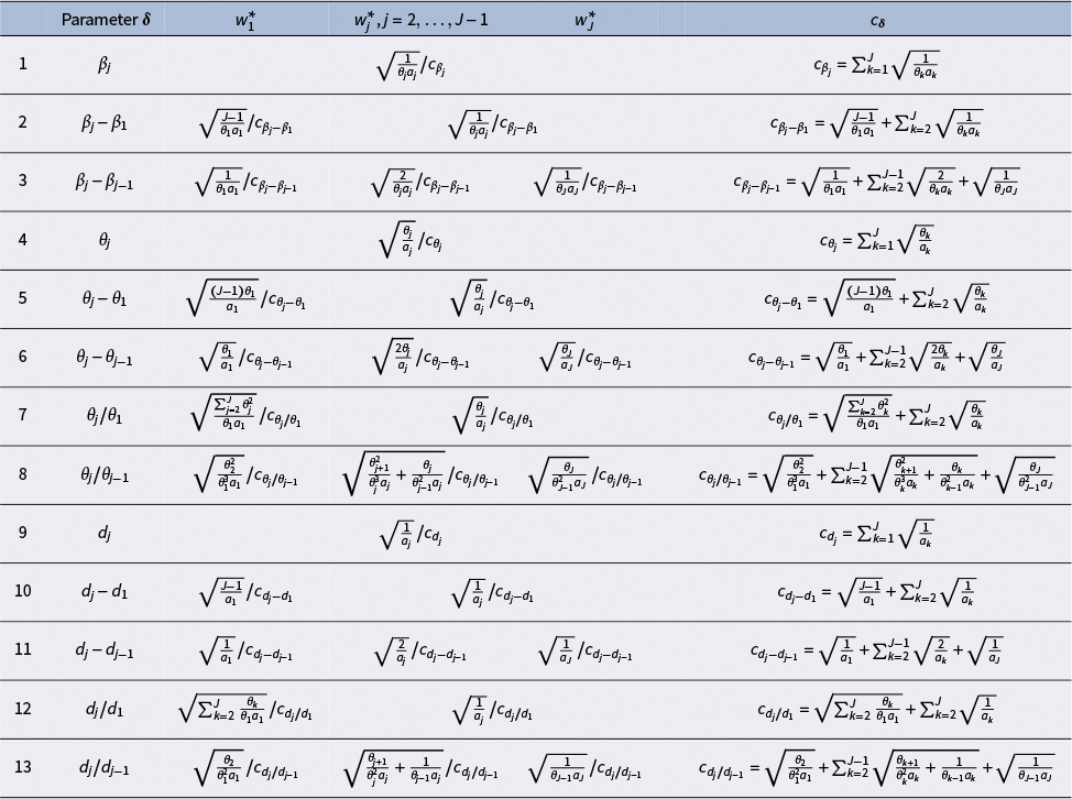
 . On this basis, we derive the corresponding quasi-information matrix. A-optimal weights for the model parameters and contrasts are then obtained from this matrix using the same procedure as for the weights reported in Table 2. The resulting weights for the extended model are given in Table A1.
The time-specific effects
$\Gamma _{ij}$
 as part of the latent variable
$\Lambda _{ij}$
 , which is decomposed as

are now assumed to be distributed as
$\Gamma (\alpha _{j}, \tau )$
 ,
$j = 1, \ldots , J$
 . Again, the permanent person effect
$\Gamma _{i0} \sim \Gamma (\alpha _0, \tau )$
 shares the same scale parameter
$\tau $
 , and all components are mutually independent.
Then, the latent variable
$\Lambda _{ij}$
 is distributed as
$\Gamma (\alpha _{0} + \alpha _{j}, \tau )$
 with mean
$\mathrm {E}(\Lambda _{ij}) = (\alpha _{0} + \alpha _{j}) \tau $
 , and the marginal mean of the responses is given by

The vector
$\boldsymbol {\Lambda }_i = (\Lambda _{i1}, \ldots , \Lambda _{iJ})^\top $
 is distributed according to a multivariate gamma distribution with
$\mathrm {Var}(\Lambda _{ij}) = (\alpha _{0} + \alpha _{j}) \tau ^{2}$
 and
$\mathrm {Cov}(\Lambda _{ij}, \Lambda _{ij'}) = \alpha _{0} \tau ^{2}$
 . Thus,

For deriving the representation of the quasi-information matrix of this extended approach
$\mathbf {M}_{\mathrm {Q}}$
 , we denote by
$\mathbf {Y}_{ij} = (Y_{ij1}, \ldots , Y_{ijn_j})^\top $
 the vector of responses of test person
$i$
 at time
$t_j$
 and by
$\mathbf {Y}_{i} = (\mathbf {Y}_{i1}^\top , \ldots , \mathbf {Y}_{iJ}^\top )^\top $
 the vector of all responses of test person
$i$
 over all
$J$
 testing occasions with first- and second-order moments

For the characterization of the inverse covariance matrix
$\mathbf {V}^{-1}$
 , we introduce

Then

With
$\mathbf {D} = \mathrm {diag}(\boldsymbol {\mu }_j)$
 and
$\mathbf {q} = (q_{1}, \ldots , q_{J})^\top $
 , the quasi-information matrix becomes

and the representation of

where
$\mathbf {a} = (1/(\alpha _0+\alpha _1), \ldots , 1/(\alpha _0+\alpha _J))^\top ,$
 follows by standard arguments of matrix inversion.
A-optimal weights for parameters and contrasts, general shape parameters
$a_j = \alpha _0 + \alpha _j$


Table A1 Long description
The table contains 13 numbered rows and 6 columns.
Column headers include: Parameter delta, w sub 1 super star, w sub j super star (where j equals 2 to J minus 1), w sub J super star, and c sub bold delta.
Key rows include:
* Row 1: Parameter beta sub j. Weight is square root of 1 all over theta sub j times a sub j all over c sub beta sub j. c sub beta sub j is the summation from k equals 1 to J of square root of 1 all over theta sub k times a sub k.
* Row 2: Parameter beta sub j minus beta sub 1. w sub 1 super star is square root of J minus 1 all over theta sub 1 times a sub 1 all over c sub beta sub j minus beta sub 1.
* Row 4: Parameter theta sub j. Weight is square root of theta sub j all over a sub j all over c sub theta sub j.
* Row 7: Parameter theta sub j all over theta sub 1. c sub theta sub j all over theta sub 1 equals square root of summation from k equals 2 to J of theta sub k squared all over theta sub 1 times a sub 1 plus summation from k equals 2 to J of square root of theta sub k all over a sub k.
* Row 9: Parameter d sub j. Weight is square root of 1 all over a sub j all over c sub d sub j.
* Row 13: Parameter d sub j all over d sub j minus 1. c sub d sub j all over d sub j minus 1 involves a summation of square roots of terms including theta sub k plus 1 all over theta sub k squared times a sub k plus 1 all over theta sub k minus 1 times a sub k.
Based on this quasi-information matrix, the A-optimal weights for the model parameters and contrasts were derived for the extended model and are represented in Table A1. It should be noted that the results in Sections 2 and 3 follow by setting formally
$\alpha _{0} + \alpha _{j} = 1$
 .



 Open access

