1. Introduction
Data assimilation (DA) refers to a class of methods designed to obtain optimised predictions of physical processes via the combination of results from multiple sources of measurements. Recent advances of this discipline in fluid mechanics (Rochoux et al. Reference Rochoux, Ricci, Lucor, Cuenot and Trouve2015; Mons et al. Reference Mons, Chassaing, Gomez and Sagaut2016; Meldi & Poux Reference Meldi and Poux2017; Chandramouli, Memin & Heitz Reference Chandramouli, Memin and Heitz2020; Zhang et al. Reference Zhang, Xiao, Gomez and Coutier-Delgosha2020, Reference Zhang, Xiao, Luo and He2022, Reference Zhang, Zhang, Li, Yang and He2024a ; Le Provost & Eldredge Reference Le Provost and Eldredge2021; Zauner et al. Reference Zauner, Mons, Marquet and Leclaire2022; Plogmann, Brenner & Jenny Reference Plogmann, Brenner and Jenny2024; Zheng et al. Reference Zheng, Fisher, Lahiri, Yoko and Juniper2024; Ephrati et al. Reference Ephrati, Franken, Luesink, Cifani and Geurts2025; Valero & Meldi Reference Valero and Meldi2025) have provided efficient guidelines of application to the analysis of complex flows, in particular for high Reynolds number regimes. While numerous studies focus principally on averaged approaches such as Reynolds-averaged Navier–Stokes (RANS) simulations, an increasing number of works deal with scale-resolved simulations such as large-eddy simulations (LES), aiming for different key objectives such as model optimisation (Mons, Du & Zaki Reference Mons, Du and Zaki2021; Moussie, Errante & Meldi Reference Moussie, Errante and Meldi2024; Zhang et al. Reference Zhang, Zhang, Li, Yang and He2024a ) or synchronisation of instantaneous flow fields (Labahn et al. Reference Labahn, Wu, Harris, Coriton, Frank and Ihme2020; Wang & Zaki Reference Wang and Zaki2022; Villanueva, Truffin & Meldi Reference Villanueva, Truffin and Meldi2024). The emergence of new approaches in this field is promising and opens future perspectives for flow analysis and control using advanced tools such as digital twins (Rasheed, San & Kvamsdal Reference Rasheed, San and Kvamsdal2020; Semeraro et al. Reference Semeraro, Lezoche, Panetto and Dassisti2021). While processes such as manufacturing and maintenance are still far from being envisioned using architectures based on scale-resolving numerical simulation, technological advancements are ready to investigate their predictive capabilities. In this framework, one of the most important open challenges is the ability to predict and potentially prevent the emergence of extreme events associated with the variability of turbulent flows. These events, which can lead to critical issues, are observed in several kinds of flows dealing with urban environments, transport engineering, and energy harvesting and production. For the latter, examples of applications severely impacted by extreme events are flow configurations for internal combustion engines. This class of flows can exhibit strong variability between cycles, which is not accurately described even by scale-resolved simulations. The possibility to infuse realistic information in the simulation process, which is one of the promising aspects of DA techniques, is therefore a key element for technological advancement in this field.
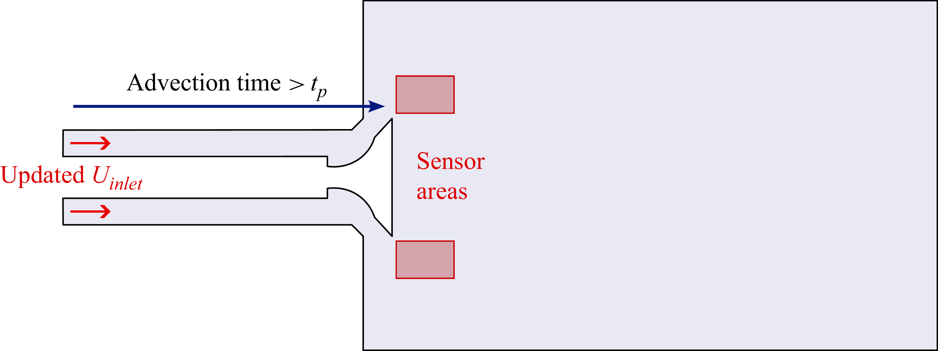
In terms of simulation of internal combustion engine flows, the steady-state flow rig is a configuration that has been studied extensively (Thobois et al. Reference Thobois, Rymer, Souleres, Poinsot and Van den Heuvel2005; Afailal et al. Reference Afailal, Galpin, Velghe and Manceau2019). In particular, this geometry is used by engine manufacturers in the early stages of development to optimise intake ducts and valve geometry. It is characterised by a single valve inserted in an intake pipe ejecting the fluid into a cylindrical chamber. The term steady-state here refers to the fact that the valve lift distance is fixed, so the geometry is motionless. This flow configuration is characterised by highly anisotropic and inhomogeneous turbulence, compressibility effects, wall effects and potentially swirl (Afailal Reference Afailal2021). The flow moving through the intake pipe and around the valve forms a jet that is affected by high shear stresses. The flow impacts the cylinder wall on either side of the valve, generating large-scale structures. As discussed previously, recent investigations studied cycle-to-cycle variations in the internal combustion engine (Ding et al. Reference Ding, Truffin and Jay2024a ,Reference Ding, Truffin and Jay b ). The cyclic variability of combustion is due to several factors. One of the most complex to identify is the variability of the intake jet, due to the intrinsically nonlinear and complex nature of unsteady turbulence combined with interactions with the walls and external fluctuations. The precise study of these events and how they originate remains difficult. Accurate representation of the behaviour of boundary conditions, which contribute to the emergence of these phenomena, could permit the study of these events relying on scale-resolved simulations. To this purpose, DA approaches show promising features to infuse experimental information into the numerical process. However, due to the complexity of the optimisation process and the large number of degrees of freedom to be considered, few studies in the literature dealing with data-informed procedures target the calibration of boundary conditions via the assimilation of locally available information.
Methods used for the prediction of inlet conditions include the minimisation of a cost function with respect to experimental data for the simulation of free-surface flows with a lattice Boltzmann method method (Nishi & Doan Reference Nishi and Doan2013), a gradient-based optimisation for a synthetic turbulence inlet condition of LES for urban flows (Lamberti et al. Reference Lamberti, García-Sánchez, Sousa and Gorlé2018), or the use of machine learning to reconstruct a hydraulic turbine suction tube inlet condition from downstream flow information for RANS simulations and LES (Véras et al. Reference Véras, Métais, Balarac, Georges, Bombenger and Ségoufin2023). In the field of DA, two studies have focused on the inference of an inlet condition in recent years. Sousa & Gorlé (Reference Sousa and Gorlé2019) use an ensemble Kalman filter (EnKF) to infer the behaviour of an inlet condition for an urban flow configuration from real measurements of anemometry data for RANS simulations. Moussie et al. (Reference Moussie, Errante and Meldi2024) target the reduction of discrepancies between scale-resolved numerical simulation and experimental measurements using the EnKF via the calibration of a synthetic turbulence inlet condition. The investigation is performed for the flow around a bluff body. These studies are developed for statistically steady test cases. To the knowledge of the authors, similar techniques have not been comprehensively explored for flows showing cyclic behaviour, which are arguably more prone to exhibit high variability of the solution and extreme events. This point is a key challenge for future applications of the digital twin paradigm for complex flows, in order to provide accurate prediction and safe control of the physical twin.
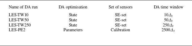
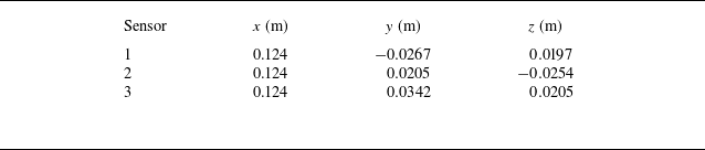
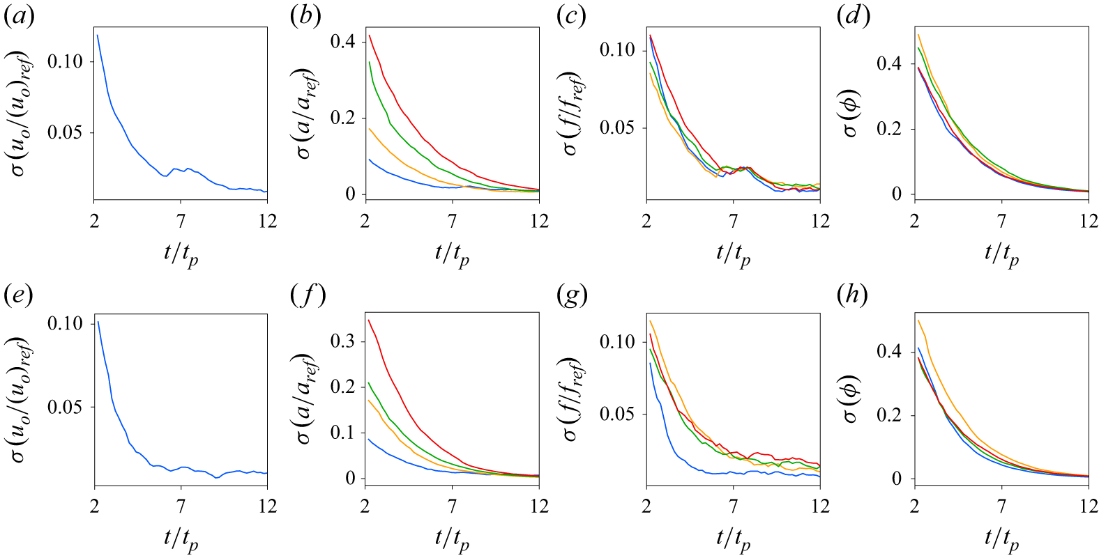
In this work, a DA strategy based on the EnKF is used to investigate a steady-state flow rig, combining high-fidelity localised data from a reference simulation with LES numerical predictions. In order to reduce the computational costs required to perform this task, a hyper-localisation procedure (HLEnKF) inspired by works in the literature is proposed. Two objectives are targeted. The first is the calibration of unsteady inlet conditions used to predict cyclic flows. The second objective deals with the synchronisation of the numerical prediction by LES with the flow configuration from which the observed data are sampled and used in the DA procedure (Villanueva et al. Reference Villanueva, Truffin and Meldi2024). The synchronisation is investigated via the analysis of instantaneous features of the flow as well as the modal behaviour of the flow. The paper is structured as follows. In § 2, the numerical tools used for the investigation are introduced and discussed. In § 3, the simulation strategies used to investigate the steady-state flow rig are validated for a simplified inlet condition using available experimental data (Thobois et al. Reference Thobois, Rymer, Souléres and Poinsot2004). In § 4, the calibration of the parameters describing an unsteady inlet condition is performed using the HLEnKF. In § 5, the DA strategy is used to investigate the efficacy of synchronisation of the velocity fields obtained with the LES runs with the observed data. In § 6, concluding remarks are provided and future applications are discussed.
2. Numerical tools
2.1. Navier–Stokes equations and numerical discretisation and modelling
Numerical simulations in this work are performed using the open-source code OpenFOAM, which relies on finite volume discretisation of the Navier–Stokes equations. For compressible flows and Newtonian fluids, they can be formulated as (Garnier, Adams & Sagaut Reference Garnier, Adams and Sagaut2009; Poinsot & Veynante Reference Poinsot and Veynante2011)
 \begin{align} \frac {\partial \rho }{\partial t} + \frac {\partial \rho u_{\!j}}{\partial x_{\!j}} &= 0, \end{align}
 \begin{align} \frac {\partial \rho u_i}{\partial t} + \frac {\partial \rho u_i u_{\!j}}{\partial x_{\!j}} &= \frac {\partial \sigma _{\textit{ij}}}{\partial x_{\!j}} - \frac {\partial p}{\partial x_i}, \end{align}
 \begin{align} \frac {\partial \rho E}{\partial t} + \frac {\partial (\rho E +p ) u_{\!j} }{\partial x_{\!j}} &= \frac {\partial \sigma _{\textit{ij}}u_i}{\partial x_{\!j}} - \frac {\partial q_{\!j}}{\partial x_{\!j}}, \end{align}
with
 $\sigma _{\textit{ij}} = - ({2}/{3}) \mu ({\partial u_k}/{\partial x_k})\delta _{\textit{ij}} + \mu ( {\partial u_{\!j}}/{\partial x_i} + {\partial u_i}/{\partial x_{\!j}} )$
and
 $q_{\!j} = -\kappa ({\partial T}/{\partial x_{\!j}})$
.
Here,
 $\boldsymbol{u}=[u_1, u_2, u_3] = [u_x, u_y, u_z]$
is the velocity field,
 $\rho$
is the density,
 $p$
is the pressure,
 $E$
is the total energy,
 $T$
is the temperature,
 $\mu$
is the dynamic viscosity, and
 $\kappa$
is the thermal conductivity. Repetition over the index
 $j$
is employed for the sake of conciseness. Numerical discretisation of (2.1)–(2.3) can be used to investigate the flow evolution. However, the complete representation of active flow scales for high Reynolds numbers demands prohibitive computational resources in terms of grid refinement. Among the approaches presented in the literature (Pope Reference Pope2000), LES (Sagaut Reference Sagaut2005) give a well-established methodology to obtain a representation of the instantaneous flow dynamics with reduced computational costs. In the LES formalism, the equations are filtered so that the large scales of motion are simulated directly, while the effects of the small filtered scales are represented by a subgrid-scale model. This operation significantly reduces the number of degrees of freedom to be simulated, therefore reducing the computational burden. The filtered compressible flow variables are typically Favre filtered or density weighted,
 $\widetilde {f} = \overline {\rho f}/\bar {\rho }$
. Assuming that the nonlinear terms in the viscous terms and in the heat fluxes are neglected (Garnier et al. Reference Garnier, Adams and Sagaut2009), the resulting equations, where
 $\bar {(\cdot)}$
indicates the filtered variables and
 $\widetilde {(\cdot)}$
the low frequency part, are
 \begin{align} \frac {\partial \overline {\rho }}{\partial t} + \frac {\partial \overline {\rho } \widetilde {u}_{\!j}}{\partial x_{\!j}} &= 0, \end{align}
 \begin{align} \frac {\partial \overline {\rho } \widetilde {u}_i}{\partial t} + \frac {\partial \overline {\rho } \widetilde {u_i} \widetilde {u}_{\!j}}{\partial x_{\!j}} &= \frac {\partial \overline {\sigma }_{\textit{ij}}}{\partial x_{\!j}} - \frac {\partial \overline {p}}{\partial x_i} -\frac {\partial \tau _{\textit{ij}}}{\partial x_{\!j}}, \end{align}
 \begin{align} \frac {\partial \overline {\rho } \widetilde {E}}{\partial t} + \frac {\partial ( \overline {\rho } \widetilde {E} +\bar p)\widetilde {u}_{\!j}}{\partial x_{\!j}} &= \frac {\partial \overline {\sigma }_{\textit{ij}} \widetilde {u}_i}{\partial x_{\!j}} + \widetilde {\kappa }\frac {\partial \widetilde {T}}{\partial x_{\!j}} -\frac {\partial q_{\!j}^{\textit{SGS}}}{\partial x_{\!j}}, \end{align}
and
 $\tau _{\textit{ij}}= \overline {\rho }(\widetilde {u_i u_{\!j}} - \widetilde {u}_i \widetilde {u}_{\!j}$
) is the subgrid-scale stress tensor. In the Smagorinsky model (Smagorinsky Reference Smagorinsky1963), the deviatoric part of
 $\tau _{\textit{ij}}$
is modelled as an eddy viscosity effect, for compressible flows:
 \begin{equation} \tau _{\textit{ij}} - \dfrac {1}{3} \delta _{\textit{ij}} \tau _{\textit{kk}} = -2 \overline {\rho } \nu _{\boldsymbol{SGS}} \left(\widetilde {S}_{\textit{ij}} - \dfrac {1}{3}\delta _{\textit{ij}}\widetilde {S}_{\textit{kk}}\right)\!, \end{equation}
where
 $\nu _{\boldsymbol{SGS}} = (C_S \varDelta )^2 \sqrt {2 \widetilde {S}_{\textit{ij}} \widetilde {S}_{\textit{ij}}}$
is the subgrid-scale viscosity,
 $\widetilde {S}_{\textit{ij}} = ( {\partial \widetilde {u}_i}/{\partial x_{\!j}} + {\partial \widetilde {u}_{\!j}}/{\partial x_i} )/2$
is the rate-of-strain tensor of the resolved velocity field,
 $\varDelta$
is the filter width, and
 $C_S$
is a model coefficient that can be selected by the user. This formulation, which is derived from the asymptotic turbulence theory by Kolmogorov, fails to provide an accurate prediction of the interactions between the resolved and filtered physical variables. The reason is that the subgrid-scale stress tensor in (2.7) is inherently dissipative and affects all the simulated scales of the flow (Sagaut Reference Sagaut2005). Here,
 $q_{\!j}^{\textit{SGS}}=\overline {\rho u_{\!j} E} - \bar \rho \widetilde {u_{\!j}} \widetilde {E}$
is the unresolved flux of the total energy. A gradient approach is used to close this term following
 $q_{\!j}^{\textit{SGS}}=-\bar \rho C_p ( {\nu _{\boldsymbol{SGS}}}/{{\textit{Pr}}_t}) ( {\partial \widetilde {T}}/{\partial x_{\!j}})$
, with the turbulent Prandtl number
 ${\textit{Pr}}_t$
set to 1.
The wall-adapting local eddy-viscosity (WALE) subgrid-scale model was developed to overcome the limitations of the Smagorinsky model, particularly in the proximity of immersed surfaces. Nicoud & Ducros (Reference Nicoud and Ducros1999) mention two main limitations of the Smagorinsky model, based on the second invariant of the symmetric part of
 $\widetilde {S}_{\textit{ij}}$
: (i) its formulation is related only to the rate-of-strain tensor and not to the rotation rate; (ii) the order of magnitude of the invariant near the wall is
 $\mathcal{O}(1)$
. The goal of the WALE model is to reproduce the expected behaviour of the subgrid-scale viscosity when approaching the wall,
 $\nu _{\boldsymbol{SGS}} = \mathcal{O}(y^3)$
, using both the rate-of-strain tensor and the rotation rate. For this, the traceless symmetric part of the velocity gradient square tensor is used:
 \begin{equation} S_{\textit{ij}}^d = \frac {1}{2} \biggl (\frac {\partial \widetilde {u}_k}{\partial x_i} \frac {\partial \widetilde {u}_{\!j}}{\partial x_k} + \frac {\partial \widetilde {u}_k}{\partial x_{\!j}} \frac {\partial \widetilde {u}_i}{\partial x_k} \biggl ) - \frac {1}{3}\delta _{\textit{ij}} \frac {\partial \widetilde {u}_k}{\partial x_m} \frac {\partial \widetilde {u}_m}{\partial x_k}. \end{equation}
The relation given by Nicoud & Ducros (Reference Nicoud and Ducros1999) can be expressed as
 \begin{equation} \nu _{\boldsymbol{SGS}} = \left(C_w^2 \varDelta \right)^2 \frac {\left(S_{\textit{ij}}^d S_{\textit{ij}}^d\right)^{3/2}}{\left(\widetilde {S}_{\textit{ij}}\widetilde {S}_{\textit{ij}}\right)^{5/2}+\left(S_{\textit{ij}}^d S_{\textit{ij}}^d\right)^{5/4}}. \end{equation}
It allows the identification of turbulent structures with high rate-of-strain and/or rotation rates. The subgrid-scale viscosity is also correctly evaluated when approaching the wall thanks to a normalisation term used in the expression (details are given in Nicoud & Ducros Reference Nicoud and Ducros1999). The implementation of the method in OpenFOAM is based on the subgrid-scale kinetic energy
 $\mathcal{K}_{\boldsymbol{SGS}}$
:
 \begin{equation} \mathcal{K}_{\boldsymbol{SGS}} = \nu _{\boldsymbol{SGS}}^2/C_k^2\varDelta ^2. \end{equation}
The width of the filter
 $\varDelta$
is also associated with the width of the geometric filter
 $\varDelta _g$
, as for the Smagorinsky model. The values of the constants can be modified by the user, by default
 $C_k = 0.094$
and
 $C_w = 0.325$
.
2.2. Bayesian DA
Discussion in § 2.1 highlighted the limitations of numerical approaches in terms of accuracy. In fact, it was shown that turbulence closures introduce a bias due to modelling structural limitations. However, even for exact subgrid-scale modelling, the evolution of instantaneous flow fields can diverge rapidly due to uncertainties affecting measurements and calculations. Even minimal variations such as machine error in computations can affect the evolution of the instantaneous field, because of the strong nonlinear, multiscale dynamics at high Reynolds number regimes (Ge, Rolland & Vassilicos Reference Ge, Rolland and Vassilicos2023). While such variations do not usually impact statistical features, they may produce desynchronisation of the flow, so that observation of instantaneous features is not reliable. In recent years, DA procedures have been used successfully to obtain flow synchronisation and to overcome some of the turbulence modelling limitations. Among the different techniques used to this purpose, variational approaches have been used extensively (Mons et al. Reference Mons, Du and Zaki2021; Ben Ali et al. Reference Ben Ali, Tissot, Aguinaga, Heitz and Mémin2022; Ghosh et al. Reference Ghosh, Mons, Sipp and Schmid2024; He et al. Reference He, Zeng, Wang, Wen and Liu2024; Wang & Zaki Reference Wang and Zaki2025). These procedures are very accurate when used to investigate physical phenomena exhibiting a clear and steady attractor for the solution, which is the case for example for applications using RANS modelling. However, potential stability issues for long observation windows (Sirkes & Tziperman Reference Sirkes and Tziperman1997) may become critical for applications to scale-resolving multiscale phenomena. This problem can be mitigated by sliding windows for observation, but it introduces complexities in the algorithm, and it is usually expensive in terms of data storage. Bayesian DA is usually less sensitive to these problems. Such methods, which can be based on ensemble representation, are usually robust when dealing with unsteady, multiscale phenomena (Asch, Bocquet & Nodet Reference Asch, Bocquet and Nodet2016).
Among the Bayesian DA techniques, the Kalman filter is a well-known DA tool first introduced in 1960 by Kalman (Reference Kalman1960) to estimate an augmented system state by combining model prediction with high fidelity but sparse external data observation. Such a DA tool is able to reconstruct a state estimation combining results from the two sources of information, as well as optimising free parameters of the model so that its predictive capabilities are augmented. One notable feature of the Kalman filter is that both sources of information are considered to be affected by uncertainties, which are modelled as Gaussian random variables. The model uncertainty
 $\boldsymbol{\eta }$
as well as the observation uncertainty
 $\boldsymbol{\epsilon }$
are therefore defined as follows:
 \begin{align} \boldsymbol{\eta }_{k+1} & \sim \mathcal{N}(0,{\boldsymbol{Q}}_{k+1}), \end{align}
 \begin{align} \boldsymbol{\epsilon }_{k+1} & \sim \mathcal{N}(0,\boldsymbol{R}_{k+1}). \end{align}
The matrices
 ${\boldsymbol{Q}}_{k+1}$
and
 $\boldsymbol{R}_{k+1}$
are the model and observation covariance matrices, respectively. The Kalman filter operates via a sequential algorithm that combines model prediction and observation via a minimisation of an error covariance matrix for consecutive state updates. The error covariance matrix
 $\boldsymbol{P}_{k+1}$
can be defined for a time
 $k = 0,1,\ldots , k_f$
as
 \begin{equation} \boldsymbol{P}_{k+1}^{f/a} = {\textrm{cov}} \left(\boldsymbol{e}_{k+1}^{f/a}\right) = E\left[\boldsymbol{e}_{k+1}^{f/a}\left(\boldsymbol{e}_{k+1}^{f/a}\right)^{\textrm{T}}\right]\!, \end{equation}
with
 \begin{equation} \boldsymbol{e}_{k+1}^{f/a} = \boldsymbol{u}_{k+1}^{f/a} - \boldsymbol{u}_{k+1}^{t}, \end{equation}
where the exponent
 $t$
(truth) indicates the true state of the physical system. The superscript
 $f$
(forecast) refers to the forecast of the state matrix obtained via the temporal advancement of the model. It is therefore the predicted state before observation is assimilated. The superscript
 $a$
(analysis) represents the final augmented state of the algorithm following the analysis phase, therefore after DA is performed. The main drawback of the classical Kalman filter consists in the costly time advancement (for the forecast) and manipulations (for the analysis) of the covariance matrix
 $\boldsymbol{P}$
. For a classical computational fluid dynamics (CFD) problem for turbulent flows, the state variables calculated on the grid may easily consist of
 $N=10^6{-}10^{12}$
degrees of freedom. The size of the error covariance matrix is therefore
 $N\times N$
, demanding prohibitive resources for its manipulation.
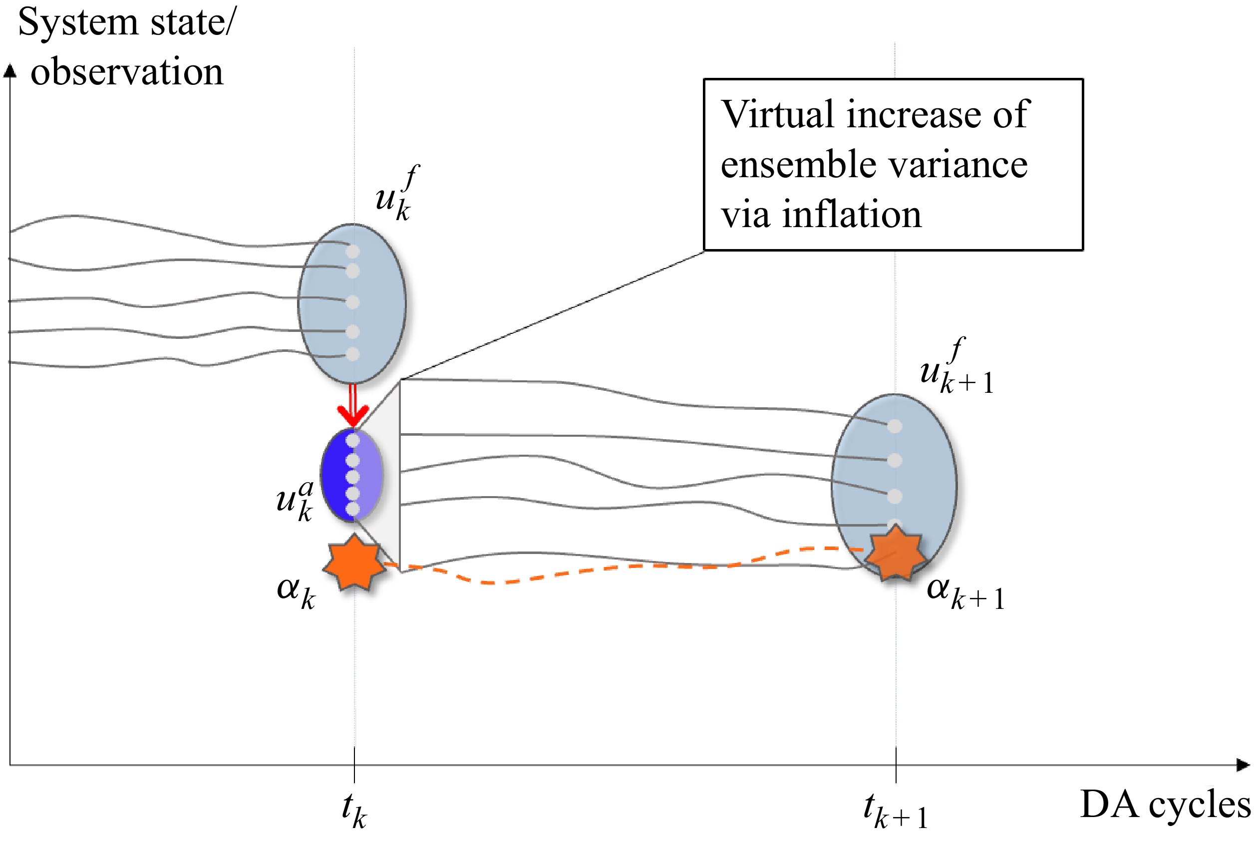
Scheme representing the EnKF. The state of the model
 $u_k^f$
is updated via the analysis phase of the EnKF algorithm by taking into account the observation
 $\alpha _k$
. Each grey line represents the trajectory of a member of the ensemble.

A strategy analysed extensively in the literature to deal with this issue is the EnKF (Evensen Reference Evensen2009). This technique has been used extensively in the field of meteorological sciences (see Asch et al. Reference Asch, Bocquet and Nodet2016) and more recently in fluid mechanics applications (Mons et al. Reference Mons, Chassaing, Gomez and Sagaut2016; Le Provost & Eldredge Reference Le Provost and Eldredge2021; Moldovan et al. Reference Moldovan, Mariotti, Lehnasch, Cordier, Salvetti and Meldi2024; Zhang et al. Reference Zhang, Zhang and He2024b
). Here, a Monte Carlo approximation is used to estimate the error covariance matrix
 $\boldsymbol{P}$
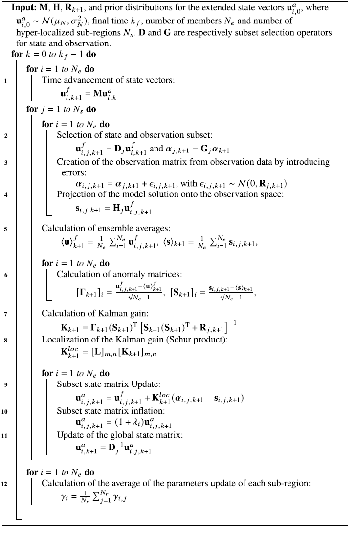
using a set of pseudo-random realisations. A simplified scheme of the EnKF procedure used in this study is presented in figure 1, and a detailed algorithm is provided in Algorithm 1. The main elements of the strategy are now discussed. The forecast step consists in the time advancement of
 $N_e$
realisations (ensemble members) using the available numerical model between successive assimilation phases. This step is exemplified by the grey lines in figure 1. If each ensemble member is described by
 $N$
degrees of freedom, then a state matrix
 $\boldsymbol{\mathcal{U}}$
of size
 $[N, N_e]$
can be assembled at the beginning of each analysis phase. Each column of such a matrix,
 $i = 1, \ldots , N_e$
, corresponds to a physical state
 $\boldsymbol{u}_i$
obtained by the
 $i$
th member of the set. The EnKF manipulates the state matrix to provide an ensemble representation of the error covariance matrix
 $\boldsymbol{P}$
, which is referred to as
 $\boldsymbol{P}_e$
, via the assumption that the ensemble members are statistically independent:
 \begin{equation} {\boldsymbol{P}}_e^{f/a} = \frac {1}{N_e-1}\sum _{i=1}^{N_e} \big(\boldsymbol{u}_i^{f/a} - \big\langle {\boldsymbol{u}}^{f/a} \big\rangle \big) \big(\boldsymbol{u}_i^{f/a} - \big \langle {\boldsymbol{u}}^{f/a} \big \rangle \big)^{\textrm{T}} = \boldsymbol{\Gamma}\boldsymbol{\Gamma}^{\textrm{T}}, \end{equation}
Algorithm of the Hyper-localized Ensemble Kalman Filter (HLEnKF)

where
 $\boldsymbol{\Gamma }$
is the anomaly matrix, which is derived from the state matrix
 $\boldsymbol{\mathcal{U}}$
. It quantifies the deviation of the state vectors from their ensemble mean:
 \begin{equation} [\boldsymbol{\Gamma }_{k+1}]_i = \frac {\boldsymbol{u}_{i,k+1}^f-\langle \boldsymbol{u}\rangle _{k+1}^f}{ \sqrt {N_e-1}} , \quad \langle \boldsymbol{u}\rangle _{k+1}^f = \frac {1}{N_e}\sum _{i = 1}^{N_e}\boldsymbol{u}_{i,k+ 1}^f . \end{equation}
The anomaly matrix plays an essential role in the state estimation. In particular, the Kalman gain
 ${\boldsymbol{K}}$
, which governs the state update of the model prediction, is obtained via manipulation of
 $\boldsymbol{\Gamma }$
and information obtained at sensors. For the latter, in order to grant an observation matrix with the same rank as the state matrix
 $\boldsymbol{\mathcal{U}}$
, the array including the
 $N_o$
available observations at time
 $k$
is artificially perturbed to obtain
 $N_e$
sets of values. More precisely, a matrix of size
 $N_o \times N_e$
is obtained by adding a bounded Gaussian noise based on the measurement error covariance matrix
 $\boldsymbol{R}_{k+1}$
to the observation vector
 $\boldsymbol{\alpha }_{k+1}$
. Each column
 $i$
of such a matrix is
 \begin{equation} \boldsymbol{\alpha }_{i,k+1} = \boldsymbol{\alpha }_{k+1} + {\epsilon}_{i,k+1},\quad \text{with} \quad {\epsilon}_{i,k+1} = \mathcal{N}(0, {\boldsymbol{R}}_{k+1}). \end{equation}
The last element of information needed to construct the Kalman gain
 ${\boldsymbol{K}}$
deals with the projection of the model prediction in the space of the sensors where observation is sampled. This operation is performed via the projection matrix
 $\boldsymbol{H}$
:
 \begin{equation} \boldsymbol{s}_{i,k+1} = \boldsymbol{H} \boldsymbol{u}_{i,k+1}^f \; . \end{equation}
In practice,
 $\boldsymbol{H}$
connects the variables calculated by the model (velocity field, pressure field, and so on) with the measured quantities that are used as observations. Therefore,
 $\boldsymbol{H}$
can, for example, be an interpolation tool (e.g. to obtain pressure values in the location of the sensors) or an integration operator (e.g. the observed quantity is the drag coefficient of an immersed body). The state estimation via EnKF is obtained as a combination of model prediction during the forecast step and the available observations. It is worth mentioning that while observation is affected by noise (see (2.17)), no model uncertainty such as that described in (2.11) is explicitly used within the algorithm. However, it is taken into account via the addition of inflation in an additional step of the algorithm (see § 2.2.1). The augmented state
 $\boldsymbol{u}_{i,k+1}^a$
is thus expressed as
 \begin{equation} \boldsymbol{u}_{i,k+1}^a = \boldsymbol{u}_{i,k+1}^f + \boldsymbol{K}_{k+1}(\boldsymbol{\alpha }_{i,k+1}-\boldsymbol{s}_{i,k+1}). \end{equation}
The way in which these two predictions are combined is governed by the Kalman gain
 $\boldsymbol{K}_{k+1}$
, here expressed at the analysis phase
 $k+1$
(Asch et al. Reference Asch, Bocquet and Nodet2016; Carrassi et al. Reference Carrassi, Bocquet, Bertino and Evensen2018):
 \begin{equation} {\boldsymbol{K}}_{k+1} = \boldsymbol{\Gamma }_{k+1}({\boldsymbol{S}}_{k+1})^{\textrm{T}} \left [{\boldsymbol{S}}_{k+1}({\boldsymbol{S}}_{k+1})^{\textrm{T}} + {\boldsymbol{R}}_{k+1}\right ]^{-1}, \end{equation}
with
 \begin{eqnarray} \left [\boldsymbol{S}_{k+1}\right ]_i= \frac {\boldsymbol{s}_{i,k+1}-\langle \boldsymbol{s}\rangle _{k+1}}{\sqrt {N_e-1}} , \quad \langle \boldsymbol{s}\rangle _{k+1} = \frac {1}{N_e}\sum _{i = 1}^{N_e}\boldsymbol{s}_{i,k+1}. \end{eqnarray}
Such EnKF-based approaches can also simultaneously optimise the free parameters governing the model to minimise the discrepancy between the model prediction and the obtained state estimation during the analysis phase. These free parameters, usually found in boundary conditions and/or turbulence closures, are stored in an array that is referred to as
 $\boldsymbol{\gamma }$
. A simple strategy to perform such an optimisation relies on the definition of an extended state (Asch et al. Reference Asch, Bocquet and Nodet2016). Here, the EnKF problem is solved for a state vector
 ${\boldsymbol{u}}_{\boldsymbol{ext}}$
defined as
 \begin{equation} {\boldsymbol{u}}_{\boldsymbol{ext}} = \begin{bmatrix} \boldsymbol{u} \\ \boldsymbol{\gamma } \end{bmatrix}\!. \end{equation}
The size of the extended state is now
 $N_{\textit{ext}}=N + N_\gamma$
, where
 $N_\gamma$
is the number of parameters to be optimised. This modification of the DA strategy results in a negligible increase in computational cost if
 $N_\gamma \ll N$
, and simultaneously provides an updated state estimation and an optimised parametric description for the model at the end of the analysis phase.
2.2.1. Hyperparameters of the EnKF: inflation
One of the major drawbacks of the EnKF is the rapid collapse of the state matrix variability. The consequence of the undesirable reduction of the variance is the convergence of the state matrix towards a localised optimum, strongly related to the provided prior state. If the latter is not well identified, which is usually the case due to lack of information, then the accuracy of the optimisation via the EnKF can be seriously affected. It is possible to increase the global variability of the system and to decrease the sampling errors by using a higher number of members in the ensemble, thus gaining accuracy in the EnKF prediction. However, this strategy is not conceivable for fluid dynamics applications where computational costs preclude the use of large ensembles. In fact, the number of members typically used for three-dimensional analyses is approximately
 $N_e \in [40,100]$
(Mons et al. Reference Mons, Du and Zaki2021; Moldovan et al. Reference Moldovan, Mariotti, Lehnasch, Cordier, Salvetti and Meldi2024), which is arguably not sufficient to ensure statistical convergence.
This problem is usually mitigated by inflating the variance of the ensemble after the analysis phase, as illustrated in figure 2. If a deterministic model is used, i.e. no uncertainty
 $\eta$
is included via (2.11), then it can be interpreted as the addition of noise to the predicted dynamic system. Inflation is usually integrated by increasing the discrepancy between each state vector
 $\boldsymbol{u}_{i,k+1}^a$
and the ensemble mean
 $\langle \boldsymbol{u}^a\rangle$
by algebraic operations driven by a coefficient
 $\lambda$
. This procedure is called multiplicative inflation. The way in which this procedure is performed can be deterministic or stochastic:
 \begin{align} {\textit{deterministic}} & \qquad \boldsymbol{u}_{i}^a \longrightarrow \langle \boldsymbol{u}^a\rangle + \lambda _i\big(\boldsymbol{u}_{i}^a-\big\langle \boldsymbol{u}^a\big\rangle \big) \quad \text{with} \quad \lambda _i \gt 1, \end{align}
 \begin{align} {\textit{stochastic}} & \qquad \boldsymbol{u}_{i}^a \longrightarrow (1+\lambda _i) \boldsymbol{u}_{i}^a \quad \text{with} \quad \lambda _i \sim \mathcal{N}(0,\sigma ). \end{align}
The deterministic implementation is usually very efficient in the initial analysis phases of the DA run. Considering that it is applied to the discrepancy of each ensemble member from the ensemble mean, this inflation is usually stable, and higher values of
 $\lambda$
can be used. However, it is less efficient when the ensemble exhibits a strong collapse of the variability of the physical solution (
 $\boldsymbol{u}_{i}^a-\langle \boldsymbol{u}^a\rangle \approx 0$
). On the other hand, stochastic inflation is efficient to avoid the collapse of the variability once the EnKF converges to a stable solution. The Gaussian distribution used to determine
 $\lambda _i$
in (2.24) is usually truncated to avoid the generation of outliers that could lead to divergence of the EnKF. Inflation is an important element in the EnKF, for which adequate tuning is often crucial. In fact, high values of inflation prevent the rapid collapse of the ensemble variability and increase the accuracy of the state estimation and the parametric optimisation, but at the same time they include noise, which may lead to the divergence of the numerical model.
Scheme representing the inflation procedure used for the EnKF. Each grey line represents the trajectory of one member of the ensemble. The increase in the variance of the ensemble via inflation is represented by the grey trapezoid.

2.2.2. Hyperparameters of the EnKF: localisation
When CFD solvers are used as models for DA procedures, the state matrix is composed of values of the flow variables (e.g. the velocity field) in correspondence with the mesh elements, usually at their centres. As shown in (2.20), the Kalman gain correlates these values with the values of the state matrix projected into the observation space, i.e. over the sensors at which observation is available. Considering that the correlation between flow variables decreases with distance in continuous systems, the approximations used to determine the Kalman gain in the EnKF framework – and in particular sampling errors – can lead to non-physical correlations in the analysed state matrix, especially for large domains. These effects can be responsible for critical issues such as unphysical flow fields leading to the divergence of the filter. Again, these problems can be reduced by increasing the number of ensemble members, therefore reducing sampling errors, which is not a viable solution for CFD applications. Therefore, different strategies must be envisioned to mitigate the effects of spurious distant correlations. Two approaches are classically adopted in the literature (Asch et al. Reference Asch, Bocquet and Nodet2016). The covariance localisation operates on the coefficients of the error covariance matrix
 $\boldsymbol{P}_{k+1}^f$
, aiming to set to zero values of model realisations sufficiently far from each sensor. This process is here performed mathematically by a Shur product between a localisation matrix
 $\boldsymbol{L}$
and the Kalman gain
 ${\boldsymbol{K}}$
. This expression can be directly included in the algorithm without any modification:
 \begin{equation} {\boldsymbol{K}_{k+1}^{loc} = [\boldsymbol{L}]_{m,n}[\boldsymbol{K}_{k+1}]_{m,n}}. \end{equation}
With
 $m$
and
 $n$
the matrices indices. The structure of the matrix
 $\boldsymbol{L}$
must be defined by the user. For fluid mechanics problems, the correlation decreases rapidly in space. Therefore, a commonly used structure for the localisation matrix is an exponential decay form
 \begin{equation} \boldsymbol{L}(m,n) = \exp\left({-\dfrac {1}{2}(\varDelta _{m,n}/l)^2}\right)\!, \end{equation}
where
 $\varDelta _{m,n}$
is the distance between the given sensor and the centre of the grid element, and
 $l$
is a correlation length scale that can be adjusted according to the local characteristics of the test case.
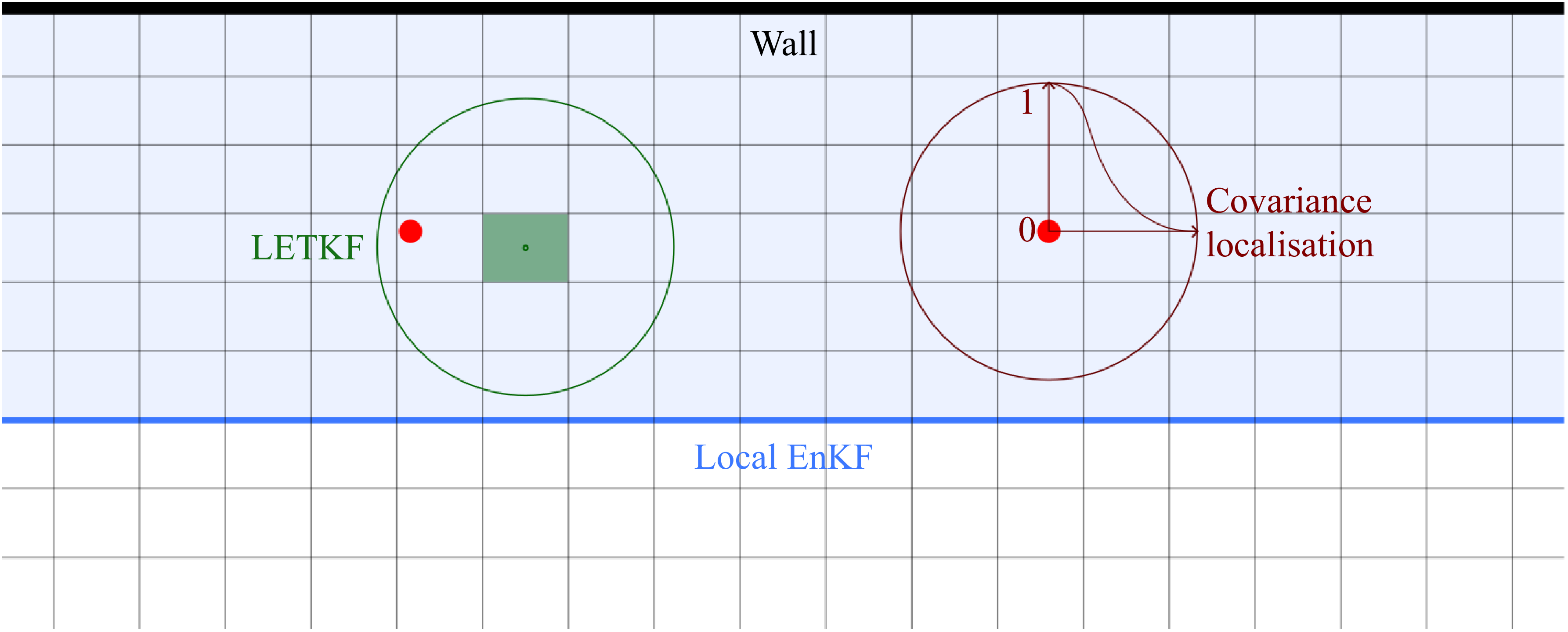
Another way to localise the Kalman gain is to use the physical localisation, also called local analysis (Evensen et al. Reference Evensen, Vossepoel and Van Leeuwen2022). Instead of running the EnKF on the entire physical domain, the computation is performed on a reduced domain. The reduced space contains all the sensors used for the sampling of observation. This strategy also has the advantage of reducing the number of degrees of freedom operating in the assimilation procedure, which can lead to a significant gain in terms of computational resources required. Covariance localisation is commonly used with physical localisation to avoid discontinuities due to the DA state update, in particular at the interface of the reduced domain. This method is very effective in simultaneously speeding up the computation and improving the computational stability and accuracy for a reduced ensemble size, such as those currently usable for CFD-based studies (Villanueva et al. Reference Villanueva, Valero, Glumac and Meldi2023, Reference Villanueva, Truffin and Meldi2024). The localisation methods described are illustrated qualitatively in figure 3.
2.2.3. Sub-setting methods
A different way to perform the localisation procedure is used in the local ensemble transform Kalman filter (LETKF) (Hunt, Kostelich & Szunyogh Reference Hunt, Kostelich and Szunyogh2007). The method consists in performing one DA procedure per cell in the domain simulated by the model. Let us consider one grid element for which the model prediction is available, generating a subset of the global state matrix
 $\boldsymbol{\mathcal{U}}_{[g]}$
. A subset of the observation vector
 $\boldsymbol{\alpha }_{[g]}$
is also generated, including observations that are within a prescribed distance from the grid element. Thus the LETKF update is a sum of
 $N_g$
local updates:
 \begin{equation} \big(\boldsymbol{u}_{i,k+1}^a\big)_{[g]} = \sum _{s=1}^{N_g} \left (\langle \boldsymbol{u}\rangle _{k+1}^f + \sqrt {N_e-1}\,[\boldsymbol{\Gamma }_{k+1}]_i\, w_i^{a}\right )_{[s]}, \end{equation}
with
 $N_g$
the number of grid elements, and
 $w_i^a$
a weight vector belonging to the ensemble space spanned by the forecast ensemble perturbations (for more details, see Hunt et al. Reference Hunt, Kostelich and Szunyogh2007). In practice, the LETKF performs one EnKF for each grid element, but the size of the state matrix is significantly reduced. Also, the observations considered for each realisation of the LETKF are only the ones included in the sub-volume considered. Despite the increase in the number of DA phases performed, the global computational costs are diminished because each of them is performed over a significantly smaller space and with fewer sensors. However, one has to deal with complex management of the discontinuities for neighbouring cells using different sets of observations. The choice of the selected
 $N_g$
cells for each iteration also requires a more complex set of hyperparameters. The method is shown qualitatively in figure 3.
Another method presented in the literature, applied to atmospheric DA, is the sequential EnKF (SEnKF) (Houtekamer & Mitchell Reference Houtekamer and Mitchell2001). The SEnKF uses a sub-setting method within the observation space. In this procedure, observations are grouped together when sensors are very close and the correlation of their measurements is known. The analysis phase becomes sequential, performing one update per observation batch. The final state is obtained as the sum of state updates provided by each of the
 $N_b$
observation batches available:
 \begin{equation} \boldsymbol{u}_{i,k+1}^{a_{N_b}} = \boldsymbol{u}_{i,k+1}^f + \sum _{j=1}^{N_b} \boldsymbol{K}_{k+1}^{a_{\!j}} \left(\boldsymbol{\alpha }_{i,k+1}^{a_{\!j}}-\boldsymbol{s}_{i,k+1}^{a_{\!j}} \right)\!. \end{equation}
The SEnKF is conceived to work efficiently with a very large number of sensors, avoiding the problem of computationally expensive matrix inversions. The procedure is not acting as a physical localisation method, even though it could be coupled to standard localisation procedures. However, it can be conceived as a procedure localising the observations and their correlations.
Simplified representation of different DA localisation methods on a Cartesian grid. The red dots represent sensors for observation. In blue: the EnKF is executed on a reduced domain. In green: application of the LETKF for one grid element. In dark red: covariance localisation is used to control the intensity of the DA state update in a given region.

2.3. Hyper-localised EnKF
A localisation procedure for the EnKF is proposed here, which is inspired by the LETKF and by the SEnKF introduced previously. The hyper-localised EnKF (HLEnKF) consists of
 $N_s$
sequential runs of a classical EnKF, where
 $N_s$
is tied to the number of sensors used in the DA procedure. More precisely, regions around the sensors are identified, and physically localised EnKFs are performed. In order to avoid discontinuity in the physical state, covariance localisation is also applied to reduce the DA state update moving towards the external surfaces of the physical regions investigated. To this purpose, (2.26) is used, tuning the free parameters so that the state update corresponds to zero at the interface of the region. The corresponding state update of the physical field can be written as
 \begin{equation} \boldsymbol{u}_{i,k+1}^a = \boldsymbol{u}_{i,k+1}^f + \sum _{s=1}^{N_s} (\boldsymbol{K}_{k+1})_{[s]}\big((\boldsymbol{\alpha }_{i,k+1})_{[s]}-(\boldsymbol{s}_{i,k+1})_{[s]}\big), \end{equation}
where the subscript
 $s$
indicates the iterations over the considered regions, and
 $[s]$
indicates the calculation of the ingredients of the EnKF (
 ${\boldsymbol{K}}$
,
 $\boldsymbol{\alpha }$
and
 $\boldsymbol{s}$
) in each of the
 $N_s$
selected physical regions. One can see a strong similarity with the LETKF, as a large number of smaller EnKFs are performed here. However, the selection for the HLEnKF is performed by creating regions around sensors for observation, not based on each grid element of the model. This latter strategy is reminiscent of the SEnKF, but in this case, the calculation of
 ${\boldsymbol{K}}$
is executed in a single operation for every DA region instead of performing (i) a first calculation in the observation space (equation 7 of Houtekamer & Mitchell Reference Houtekamer and Mitchell2001) and (ii) a second transformation of the forecast model (equation 8 of Houtekamer & Mitchell Reference Houtekamer and Mitchell2001). Therefore, the state correction is directly projected on the model space via a single calculation that is limited to the DA region of interest. Additionally, the
 $s$
state updates can be performed in parallel with respect to the forecast of the solution, while the SEnKF procedure is sequential. This implies that (i) potential problems arising in the order of the DA state updates are excluded, and (ii) the procedure can be performed in parallel calculation, providing a further boost in speed.
The number of regions
 $N_s$
is now discussed. If sensors are physically far one from each other, then
 $N_s$
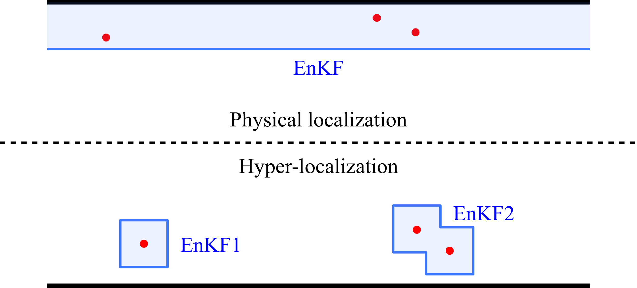
is equal to the number of sensors, i.e. each DA physical region is centred around a sensor. This choice precludes the possibility to include the correlation between the observations measured at different sensors. Arguably, this apparent drawback can actually help to stabilise the performance of the filter, as the correlation between variables measured at distant locations can be affected by large errors. In case some sensors are clustered in a physical region, the algorithm is able to combine regions identified around one sensor, and to perform one EnKF using a batch of close observations. A qualitative comparison between classical physical localisation and hyper-localisation is shown in figure 4. One key element governing the efficiency of this approach is clearly the size of the DA region around the sensors. A small region grants reduced computational resources and exhibits smaller sampling errors. This approach becomes a nudging approach if the region considered consists of the location of the sensor. On the other hand, large regions allow the DA state update to influence a greater portion of the domain, thereby accelerating parametric optimisation and enhancing flow synchronisation. In the present work, the regions are selected to be of spherical form around each sensor. The diameter of such spheres is proportional to the integral length scale of the flow. While this criterion is adequate for the analysis of turbulent flows, such as the test case presently investigated, it does not necessarily apply to other flow configurations such as convection-dominated flows. The team is currently performing investigations about physics-based criteria to determine the size and shape of the DA region that are, however, outside the scope of the present work. More details about this important aspect are provided in § 5.
Scheme representing the principle of hyper-localisation. The red dots represent sensors for observation. A local EnKF is performed around each sensor (EnKF1). In case some sensors are close, surrounding regions are combined (EnKF2). A comparison is shown with classical physical localisation (EnKF).

Finally, the parametric optimisation procedure is discussed. The HLEnKF provides
 $N_s$
values for each optimised coefficient. In the present work, global values are obtained by averaging the
 $N_s$
optimised coefficient by each local EnKF. This strategy, which was extensively investigated in preliminary studies (Villanueva Reference Villanueva2024, Appendix B), shows a robust convergence of the parametric optimisation at the expense of a slightly slower convergence rate. Another notable advantage of the HLEnKF procedure is the computational efficiency. The usage of localised regions for the DA procedure permits the manipulation of smaller arrays and matrices, reducing the total computational costs while preserving similar levels of accuracy when compared with the classical implementation of the EnKF (Villanueva Reference Villanueva2024, Appendix B). This is particularly true for physical systems described by numerous degrees of freedom, such as the numerical simulations performed in this work.
2.4. The CONES library: coupling openFOAM with numerical environments
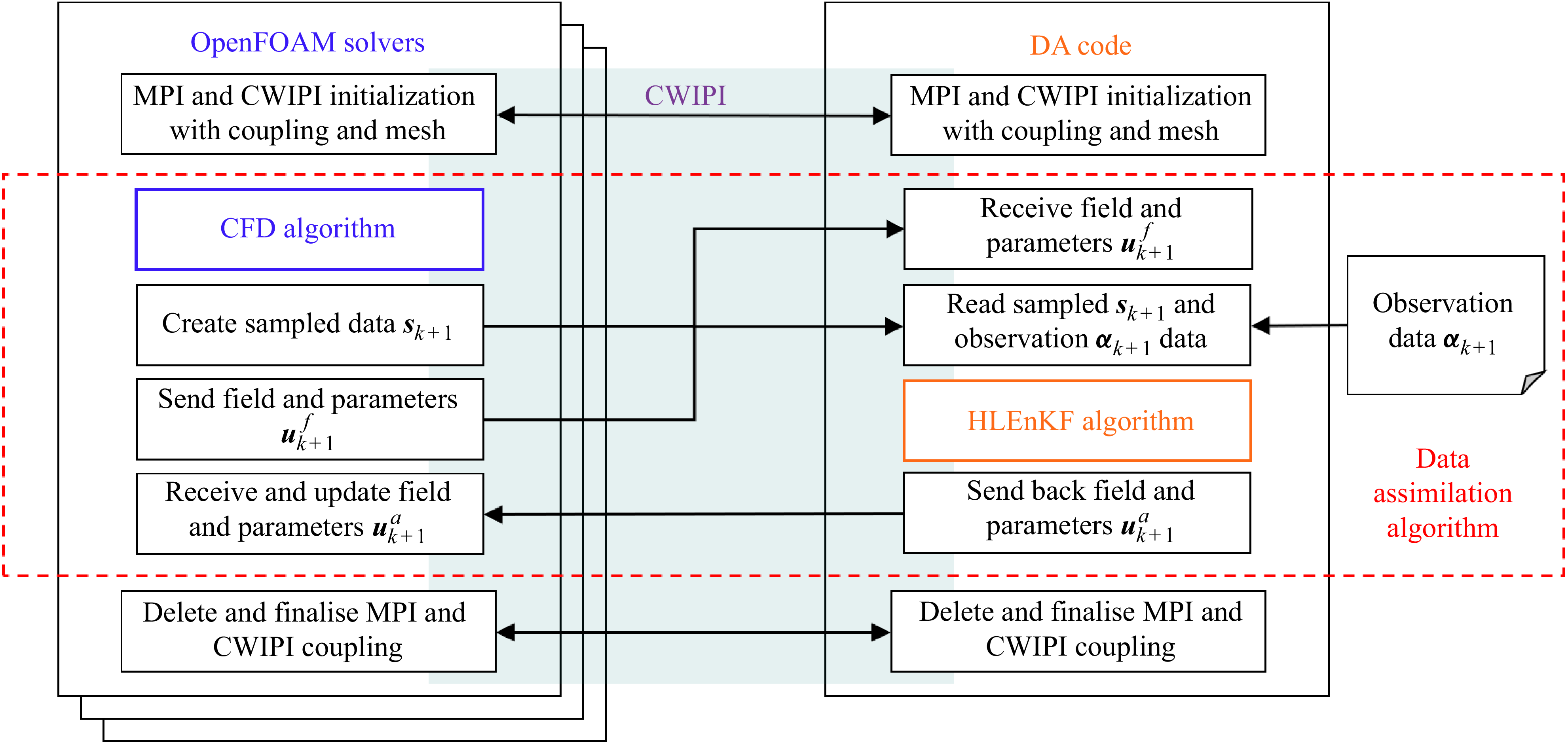
The CONES (coupling OpenFOAM with numerical environments) library is a DA library developed for online applications. It is tailored to perform online coupling between results from numerical calculations performed with the code OpenFOAM and available observations. The latter can be obtained from available repositories as well as from sensors sampling data in real time. The tool relies on an existing coupler, called CWIPI, developed by CERFACS and ONERA French laboratories (Reflox et al. Reference Reflox2011). The DA using an ensemble sequential algorithm requires multiple online simultaneous calculations as well as the processing of their results in the EnKF algorithm. Then CONES is able to transfer complete physical fields, such as the velocity field, between the OpenFOAM runs and the DA code. The ensemble CFD computations are online, and they are paused during data transfer and DA analysis. This implies that stop and restart of the numerical simulations is avoided, greatly enhancing the efficacy of the procedure in computational terms. Figure 5 summarises the operations of CONES, and in particular the coupling performed by CWIPI. In this analysis, the HLEnKF algorithm, which is performed computationally by one core, is coupled with
 $N_e=35$
CFD realisations (ensemble members). Each simulation is performed using 52 cores, for a total of 1821 cores used for each DA experiment. The steps of the algorithm presented in § 2.2 are implemented in this way within CONES.
-
(i) First, the forecast step is performed by the CFD solver until the time of the first analysis phase. This step includes the time advancement of every simulation of the ensemble.
-
(ii) The second step corresponds to the beginning of the DA analysis phase:
 $N_e$
velocity fields are sent to the DA code by the ensemble members. The information is assembled to form a single large matrix (state matrix using the DA formalism). In addition, the same physical field is interpolated to the coordinates of the sensors used for the observations, in order to obtain the term
$s_{k+1}$
in (2.19) for each ensemble member.
-
(iii) Similarly, the set of parameters to be optimised, which is included in the extended state matrix, is sent using MPI primitives. Several functions in CONES handle the exchange of different parameters (model constants, boundary conditions, and so on).
-
(iv) Observation vectors are prepared. In the present analysis, data are read from the files in the available database.
-
(v) The analysis phase is performed, including the run of the HLEnKF and the update of the extended state matrix.
-
(vi) Finally, the information stored in the extended state matrix is sent back to the ensemble members, and the physical fields are updated. Calculations will resume until the next analysis phase until the end of the DA experiment.


In the present analysis, the state update is restricted to the velocity field. The other flow fields (pressure, density and temperature) are updated via one run of the same equations used in the PIMPLE loop used in OpenFOAM, based on the inferred velocity field via DA. The DA state update term, which is usually small after a couple of analysis phases, is propagated to the other variables in a few iterations via the numerical resolution of the solver (Meldi & Poux Reference Meldi and Poux2017). This choice is performed to reduce the global cost of the DA procedure, but also to grant physically consistent fields at each time step. When finalising the computation, the couplings must be completed, and the CWIPI and then MPI environments must be finalised.
Representation of the different tasks of the library CONES. Left: each call of an OpenFOAM solver represents one member of the ensemble. Right: in-house code performing the DA update at each analysis phase. Middle: CWIPI coupler allowing communication between the running algorithms.

3. Test case set-up
The flow rig test case is now described. The present DA investigation completely relies on numerical tools, and extended discussion about the choices performed for the model and the observation will be provided.
3.1. Validation for a steady flow configuration
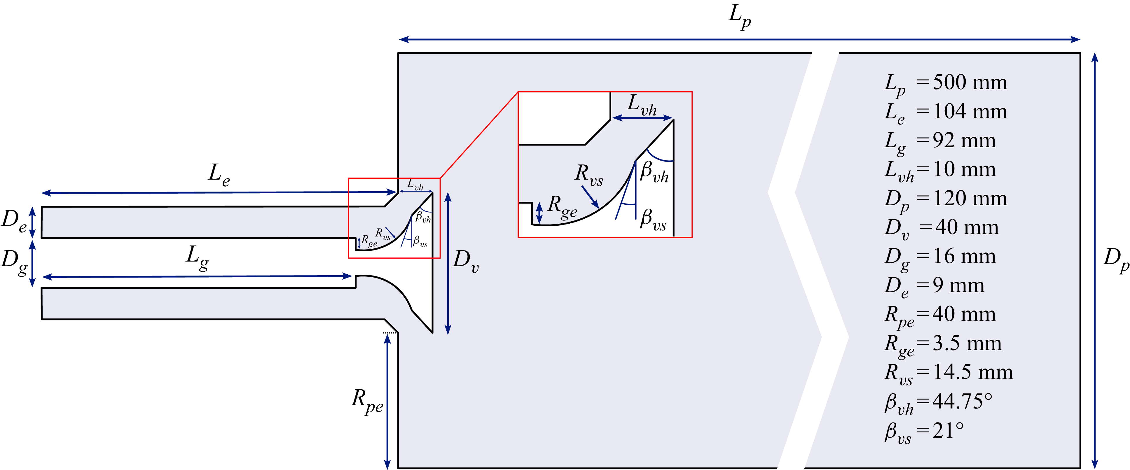
The physical domain investigated is a simplified engine geometry referred to as the flow rig. This configuration has been investigated previously in several numerical studies, in particular for LES (Graftieaux, Michard & Grosjean Reference Graftieaux, Michard and Grosjean2001; Thobois et al. Reference Thobois, Rymer, Souléres and Poinsot2004; Nicoud Reference Nicoud2018; Afailal et al. Reference Afailal, Galpin, Velghe and Manceau2019), and it is inspired by the asymmetric expansion studied by Dellenback, Metzger & Neitzel (Reference Dellenback, Metzger and Neitzel1988) for the measurement of a swirled turbulent flow. The geometric features of the test case are shown in figure 6. It consists of an inlet pipe with a guide and an open valve, which leads the flow towards a cylindrical combustion chamber. The geometry does not change over time, meaning that the valve stays in a fixed position. This flow configuration is representative of the intake in a spark-ignition engine, and it is commonly used in early development phases by engine manufacturers to optimise pipe dimensions, valve shapes, and even flow rotation levels (Thobois et al. Reference Thobois, Rymer, Souléres and Poinsot2004). The geometric features are indicated on the scheme. The main characteristics to be summarised are the diameter of the valve
 $D_v = {40}\,{\textrm{mm}}$
, the radius of the outlet chamber
 $R = D_p/2 = {60}\,{\textrm{mm}}$
, and its length
 $L_p = {500}\,{\textrm{mm}}$
, as well as the length of the inlet pipe
 $L_e = {104}\,{\textrm{mm}}$
. The head of the valve is at a distance
 $L_{vh} = {10}\,{\textrm{mm}}$
from the end of the inlet pipe. The origin of geometry
 $(x,y,z)=(0,0,0)$
is located on the axis of revolution of the cylinders on the inlet plane at the beginning of the inlet pipe.
Geometric features of the steady-state flow rig test case representing a simplified engine geometry.

A preliminary simulation for this test case is run with the objective of validating the numerical set-up against available experimental data. The latter have been obtained from Thobois (Reference Thobois2006), who performed velocity measurements by laser Doppler anemometry on the same geometry of the flow rig and with a constant mass flow rate. We refer to this configuration as steady inlet. The solver used for the preliminary numerical run is rhoPimpleFoam from OpenFOAM, which is tailored for the simulation of compressible flows using the PIMPLE algorithm. A second-order implicit scheme is used for the time advancement of the solution. The time step of the CFD calculation is
 $\varDelta _t = {2\times {10}^{-8}}\,{\textrm{s}}$
, which grants a Courant–Friedrichs–Lewy (CFL) condition
 $\textit{CFL}\lt 0.5$
. Second-order centred schemes were used for the discretisation of the spatial derivatives, except for the velocity transport term in the momentum equation, for which a LUST scheme has been prescribed. This native OpenFOAM scheme combines a second-order centred scheme and a second-order upwind scheme with ratio
 $75$
–
 $25\,\%$
. Only the air flow is studied, and transport of passive–active scalars is not included. The fluid is considered an ideal gas. Its initial properties, which are selected for
 ${21.85}\,^\circ {\textrm {C}}$
, are imposed in the OpenFOAM configuration files, as follows: molar mass
 $M^{mol} = {28.9}\,{\textrm{g mol}}^{-1}$
, specific heat at constant volume
 $C_v = {718}\ \textrm {kJ}\ {\textrm {K}^{-1}}$
, dynamic viscosity
 $\mu = {1.82\times {10}^{-5}}\ \textrm {kg} {\ \textrm {m}}^{-1} {\ {\textrm{s}}}^{-1}$
, as well as Prandtl number
 $\textit{Pr} = 0.708$
. The wall condition is a no-slip condition. For the velocity, the outlet condition pressureInletOutletVelocity specifies a zero gradient based on the dynamic pressure without recirculation of the flow. The condition waveTransmissive is imposed at the outlet for the pressure field with reference pressure
 $p_{\textit{atm}} = {101\,325}\ \textrm {Pa}$
. It prevents the reflection of waves inside the domain. The pressure gradient is zero at the inlet. A fixed temperature
 ${295}\,\textrm {K}$
is imposed at the inlet, and the temperature gradient is zero at the outlet. The axial bulk velocity imposed at the inlet is selected using the mass flow rate
 $Q_m = {0.055}\,\textrm {kg}{\,{\textrm{s}}}^{-1}$
as in the experiments by Thobois (Reference Thobois2006). A uniform velocity
 $U_{\textit{inlet}}= u_b = \iiint _{V_D} u_x \, {\textrm{d}}V^{\prime } / V_D = {65}{\,\textrm {m}}{\,{\textrm{s}}}^{-1}$
is therefore applied at the inlet. The Reynolds number calculated using the diameter of the intake annular duct is
 ${Re} = 37\,500$
. The grid used to perform this simulation, which is shown in figure 7, is composed of
 $131 \, 764 \, 400$
elements. It was generated using the blockMesh tool of OpenFOAM. It is structured and composed of hexahedral elements. The size of the grid is a priori calibrated so that the size of the elements at the wall of the intake pipe is
 $\Delta r_1^+ = r/\delta _{\nu } = r u_{\tau }/\nu \approx 1$
, where
 $u_\tau = \sqrt {\tau _w/\rho }$
is the estimated friction velocity, and
 $\tau _w$
is the shear stress at the wall. The size of the grid elements then progressively increases moving away from the walls. Subgrid-scale modelling is performed using LES with the WALE turbulence model, as presented in § 2.1. For validation in the steady case, the calculation of the velocity averages is performed for a duration of
 $8$
advective times with
 $t_A = D_e/u_b$
after the effects of initial conditions are dissipated. The analysis of the rate of convergence of the statistics indicates that this average time grants convergence error lower than
 $5\,\%$
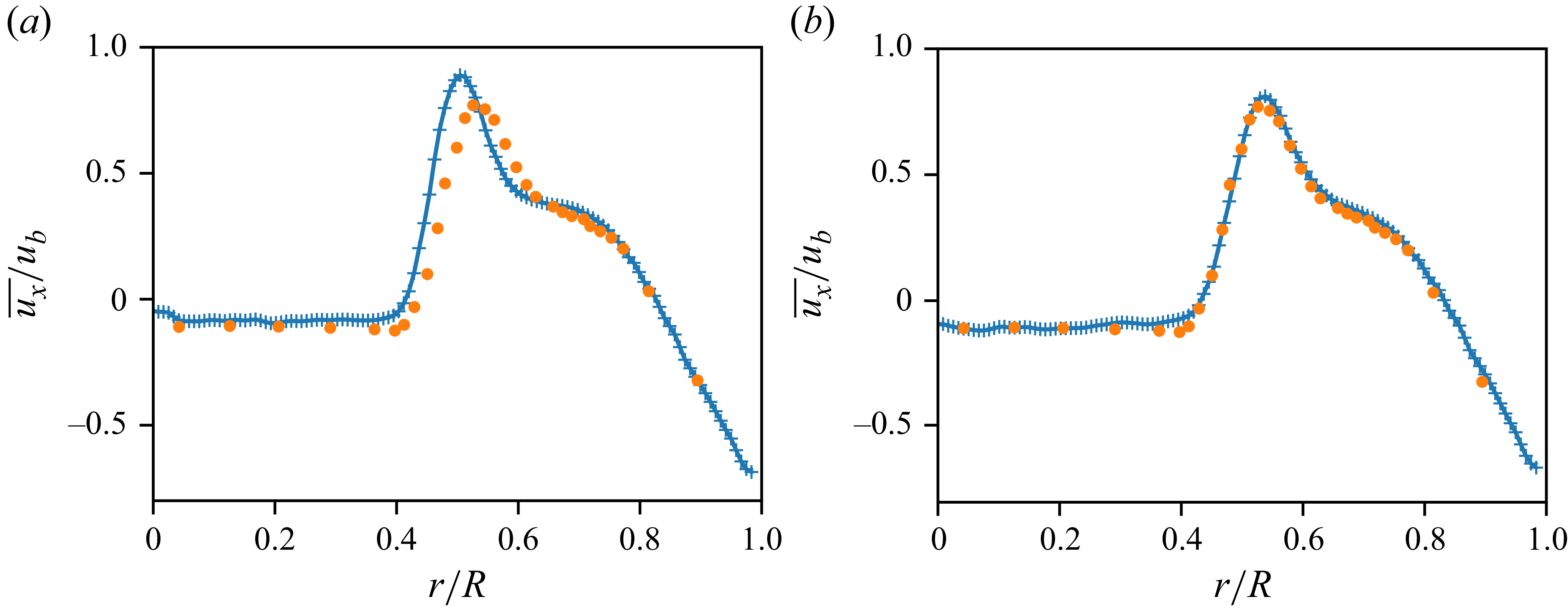
, which was estimated to be an acceptable precision level for this initial validation, in particular because a steady inlet condition is not used in the DA experiment. Figure 8 shows the radial profile of mean axial velocity normalised by the bulk velocity
 $\overline {u_x}/u_b$
. The averages
 $\overline {\cdot}$
are performed in time as well as in the azimuthal direction. Experimental data (orange dots), given at a section for
 $x={0.124}\,\textrm {m}$
, are compared with numerical data (blue crosses) taken at a section for
 $x={0.124}\,\textrm {m}$
(figure 8
a) and at a section for
 $x={0.126}\,\textrm {m}$
(figure 8
b). One can see that experiments and numerical data exhibit good agreement if a small uncertainty in the positioning of the experimental measurements and in the spatial development of the predicted separated region is considered. This comparison assesses the validity of the numerical set-up used for this case, which will be used for both the model and the production of the observation in the DA procedure.
Details of the structured grid used for the reference high-fidelity simulation (LES-HF).

Normalised axial velocity profiles for two sections at (a)
 $x = {0.124}\,\textrm {m}$
and (b)
 $x = {0.126}\,\textrm {m}$
. Experimental data from Thobois et al. (Reference Thobois, Rymer, Souléres and Poinsot2004), shown as orange dots, are compared with results from the high-fidelity LES-HF, which are reported in blue.

3.2. Production of observation: reference high-fidelity simulation (LES-HF)
The test case validated via the comparison with experimental data is used to (i) produce heterogeneous samples to be used as observation in the DA experiment, and (ii) obtain reference statistics to assess the accuracy of the DA algorithm. However, modifications are performed as the DA analysis targets flow reconstruction and parametric optimisation for cyclic phenomena such as those observed in internal combustion engines. While no modifications of the geometry are performed, a pulsating mass flow rate condition at the inlet is instead considered to induce periodicity of the flow. This condition is obtained via a modification of the velocity at the inlet such that
 \begin{equation} U_{\textit{inlet}} = a_{\textit{ref}} \sin(2\pi f_{\textit{ref}} \, t + \phi _{\textit{ref}}) + U_o, \end{equation}
where
 $U_o = u_b$
corresponds to the average velocity at the inlet. The phase
 $\phi _{\textit{ref}}$
is set to zero. The amplitude is set to consider a maximum variation of
 $\pm 15\,\%$
of the inlet velocity, therefore
 $a_{\textit{ref}} = {9.75}\,\textrm {m}{\,{\textrm{s}}}^{-1}$
. The reference frequency
 $f_{\textit{ref}} = {800}\,\textrm {Hz}$
used here is approximately 6–10 times higher than the characteristic frequencies of the pressure and velocity signals in the intake pipes linked to the propagation of acoustic waves (Pera & Angelberger Reference Pera and Angelberger2011; Leite et al. Reference Leite, Laignel, Brequigny, Borée and Foucher2023). This choice was made in order to perform the DA investigation over an increased number of cycles, which otherwise would have demanded prohibitive computational resources to be performed. The period of a complete oscillation for the velocity at the inlet is
 $t_p={1.25\times 10^{-3}}\,{\textrm{s}}$
, and we recall that the time step is
 $\varDelta _t = 2 \times 10^{-8}$
s. The simulation is run for total time
 $10 t_p$
using as initial condition an instantaneous flow field taken from the preliminary steady simulation.
Locations of the sensors used to measure the evolution of velocity and pressure in the intake channel (red dots). The two-dimensional section for
 $x={0.124}\,\textrm {m}$
used for data sampling is shown in green. Data extracted on these geometric locations are used for validation comparing results with the LES-HF run.

Evolution of (a) the normalised axial velocity
 $u_x / u_b$
and (b) the normalised pressure
 $p / p_{\textit{atm}}$
for the run LES-HF. The values are given for the three sensors located along the intake duct for
 $x = 0$
(light blue),
 $x={0.046}\,\textrm {m}$
(dark blue) and
 $x={0.092}\,\textrm {m}$
(purple) reported in figure 9.

The evolution of the velocity and the pressure fields in the intake pipe is investigated using probes positioned at the centreline (see figure 9). The three sensors are positioned at the inlet, halfway through the intake pipe and in proximity to the valve. Figure 10 shows the evolution of velocity and pressure on the three sensors investigated. Light blue data, which are sampled on the inlet boundary condition, clearly show the periodic behaviour at the centreline. Moving downstream, one can also see that the velocity fluctuations increase in magnitude (up to
 $60{-}70\,\%$
of the bulk velocity) and the pressure exhibits higher frequency fluctuations. The pressure fluctuations sampled at the end of the intake pipe also seem to indicate that the signature of the initial conditions lasts for the first six cycles. Therefore, DA analyses in §§ 4 and 5 are performed using observations sampled from cycles
 $7$
–
 $10$
, in order to avoid transient effects that could have an impact on the conclusions drawn.
Instantaneous velocity field for the run LES-HF for
 $t=9 t_p$
on the section
 $z = 0$
. The pressure field is shown on the surface of the valve. Recirculation regions are visible on each side of the jet. Flow variations visible in the intake pipe are due to the time-varying inlet boundary condition.

Figure 11 shows the instantaneous velocity field in the domain for a plane sampled for
 $z = 0$
. In addition, the normalised pressure is shown on the surface of the guide and the valve. Values have been selected from a flow snapshot selected during the ninth cycle. An annular recirculation region is visible in the proximity of the valve at the end of the intake pipe. The flow moving through the valve curtain behaves similarly to a flow through a contraction, leading to acceleration. Flow separation at the valve head alters the flow structure (Annand & Roe Reference Annand and Roe1974). Downstream of the valve, the axisymmetric flow structure is similar to that of a confined bluff-body flow evolving through a sudden expansion (Ayache et al. Reference Ayache, Dawson, Triantafyllidis, Balachandran and Mastorakos2010; Massey, Langella & Swaminathan Reference Massey, Langella and Swaminathan2019). It features a large inner recirculation zone formed by two counter-rotating vortices. Additionally, upon impacting the wall, the jet generates a wall-bounded recirculation zone, also known as an outer recirculation zone. Sharp axial and tangential velocity gradients exist between the recirculation zones and the jet, creating regions of high shear that reattach to the wall. A detailed description of the flow topology for this specific configuration is provided by Thobois et al. (Reference Thobois, Rymer, Souléres and Poinsot2004, Reference Thobois, Rymer, Souleres, Poinsot and Van den Heuvel2005) and Afailal et al. (Reference Afailal, Galpin, Velghe and Manceau2019). The effects of the periodic inlet boundary conditions are also visible in the intake pipe, with important gradients of the velocity field in the
 $x$
direction.
Position of the sensors used for the sampling of observations on LES-HF. The sensors (orange dots) are positioned over five sections, for
 $x = {0.124}\,\textrm {m}$
,
 $x={0.144}\,\textrm {m}$
,
 $x={0.164}\,\textrm {m}$
,
 $y=0$
and
 $z=0$
.

As indicated at the beginning of this subsection, the LES-HF have two main purposes. First, instantaneous data are sampled during cycles 7–10 to create observations. Most of the measurements are performed in the cylinder region, and in particular sampling is performed using the two-dimensional planes for
 $x = {0.124}\,\textrm {m}$
,
 $x={0.144}\,\textrm {m}$
,
 $x={0.164}\,\textrm {m}$
,
 $y=0$
and
 $z=0$
. In order to have the possibility to test several configurations, a total of
 $56 \, 226$
sensors are used for the measurements, whose distribution is shown in figure 12. While not all the data stored during the realisation of this simulation have been used for the DA runs in this work, the database will be used in future analysis, and it will be made available using dedicated platforms. Details about the sampling strategy are now provided. In terms of spatial distribution, the sensors’ density is higher in the region of the jet exiting the intake duct. The velocity is sampled at the sensor positions every
 $\varDelta _{\textit{tm}} = 50\varDelta _t = {1\times {10}^{-6}}\ {\textrm{s}}$
. This corresponds to
 $1250$
samples per cycle, therefore
 $t_p = 1250\, \varDelta _{\textit{tm}} = 62 \, 500\, \varDelta _t$
. A qualitative study of the flow fields seems to indicate that the size of the resolved eddies in the valve region is of the order of
 ${5\times {10}^{-4}}\,\textrm {m}$
up to
 ${5\times {10}^{-3}}\,\textrm {m}$
for the largest coherent structures. Approximated values for the turnover time obtained via classical theoretical and dimensional arguments seem to indicate that the chosen sampling frequency corresponds to
 $8{-}80$
measurements for the resolved turbulent structures. The sampling frequency is therefore sufficient to capture the dynamic structures observed. Thus problems in respecting the Nyquist–Shannon sampling theorem that could have an impact on the accuracy of the DA procedure (Meldi Reference Meldi2018) should be excluded here.
3.3. Numerical model for ensemblistic DA: low-fidelity simulation
The numerical solver used as a model for DA purposes is now presented. This model is going to use the same flow solver with the same specifications of LES-HF in terms of numerical schemes, subgrid-scale closure and boundary conditions, but it will be run on a significantly coarser grid, for two reasons. First, an ensemble of realisations as required by the EnKF would require prohibitive computational costs when using the grid prepared for the run LES-HF. Second, one of the points of interest of this work is to investigate how DA’s parametric investigation and state estimation are affected by different levels of bias in the model and in the observation. This low-fidelity model will be referred to as LES-LF (low fidelity). The main characteristics are summarised in table 1 with the LES-HF reference run. The grid used for calculation consists of
 $8 \, 764 \, 400$
elements. The structure of the grid is very similar to that used for the run LES-HF, but the number of elements is reduced by approximately a factor of
 $15$
. This time, the size of the near-wall grid elements is adjusted so that
 $\Delta r_1^+ = r/\delta _{\nu } = r u_{\tau }/\nu \approx 4{-}5$
, meaning that the simulation in the intake pipe is no longer wall-resolved. However, considering that the first grid element is included in the sub-viscous region, and that a WALE closure is selected, it was decided not to include a wall model. Grid elements are also significantly less resolved in the valve and cylinder area, therefore precluding the direct resolution of small eddies and relying on a stronger contribution of the WALE closure. This can be observed clearly by comparing the mean subgrid-scale viscosity between the runs LES-HF and LES-LF, which is shown in figure 13. The mean subgrid-scale viscosity field
 $\overline {\nu _{\boldsymbol{SGS}}}$
normalised by the initial kinematic viscosity
 $\nu _{\textit{init}}$
is approximately twice as high downstream of the valve for LES-LF compared to LES-HF. Consequently, the flow dynamics differs due to the stronger diffusive effect of the subgrid-scale closure.
Summary of the main grid and simulation features for the runs LES-HF (high-fidelity) and LES-LF (low-fidelity).

Mean subgrid-scale viscosity field normalised by the initial kinematic viscosity
 $\nu _{\boldsymbol{SGS}}/\nu _{\textit{init}}$
in the proximity of the open valve. Results are shown on a section for
 $z=0$
for (a) the LES-HF run and (b) the LES-LF run.

Differences between LES-HF and LES-LF are also observed when comparing data sampled from the three sensors positioned in the intake pipe. Once the effects of the initial conditions are dissipated, the velocity oscillations in the intake duct exhibit higher variations for the case LES-LF, as shown in figure 14. This time, the maximum velocity reached at the end of the intake duct exhibits oscillations up to
 $+ 100\,\%$
relative to the bulk velocity. On the other hand, the minimum of the oscillation goes down to
 $50{-}60\,\%$
of
 $u_b$
. The maximum and minimum values for the velocity field are observed at the sensor located at the end of the intake pipe, just before the valve region. It also seems that, on average, the flow at the centreline exhibits a non-negligible acceleration moving downstream from the inlet, which was not observed for the run LES-HF. This important dynamic difference affects the development of the jet moving from the valve to the cylinder, and it confirms the strong sensitivity of LES to changes in the grid used (Sagaut Reference Sagaut2005). This point will also be investigated extensively via the analysis of the DA results.
Evolution of (a) the normalised axial velocity
 $u_x / u_b$
and (b) the normalised pressure
 $p / p_{\boldsymbol{atm}}$
for the run LES-LF. The values are given for three sensors located along the intake duct for
 $x = 0$
(light blue),
 $x={0.046}\,\textrm {m}$
(dark blue) and
 $x={0.092}\,\textrm {m}$
(purple) reported in figure 9.

4. Calibration of inlet boundary conditions via DA
The EnKF algorithm is used here to calibrate the features of the inlet boundary conditions for an ensemble of numerical simulations based on the model LES-LF. More precisely, the free coefficients governing the parametric description of the inlet velocity field will be optimised in an online procedure to reduce the discrepancy of the prediction of the ensemble run with local data sampled from LES-HF. The inlet boundary condition of the latter is supposed to be unknown, and its effects are only measured by the measurements that are obtained downstream at the sensors and used as observation. Multiple analysis phases are performed comparing instantaneous flow snapshots, permitting an optimisation process that can naturally evolve in time with the sequential analysis phases. It is important to stress that the possibility to account for fine features in boundary conditions is one of the main limitations of scale-resolving numerical approaches to reproduce instantaneous features of real applications. Therefore, DA optimisation represents here a key element to create a solid bridge between the physical and numerical entities towards the establishment of a digital twin paradigm.
4.1. The DA experiment
The first assumption here is that the inlet velocity profile of (3.1) is unknown, and only limited measurements from the physical representation of LES-HF are available. Therefore, the calibration performed via the DA procedures aims to reconstruct global information from an ensemble of numerical realisations and limited observed measurements. The optimisation of the features of the inlet is performed using the HLEnKF algorithm presented in § 2.3. The DA procedure performed here aims for a parametric optimisation of the inlet boundary condition without including a state update. This approach is intended to provide insights into the performance of DA optimisation when using instantaneous data at high Reynolds numbers, where strong fluctuations are present. The inclusion of state estimation would have significantly increased the complexity of the procedure, not only in terms of the features to be considered, but also in ensuring the stability of the numerical system. The ingredients used in the present DA procedure are now introduced.
-
(i) A model is used in the forecast steps to propagate the solutions of the ensemble members in time. The numerical model employed for this purpose is the same as that used for LES-LF. In particular, a coarse grid of approximately
$8 \times10^{6}$
elements is used for the calculations. Each of the ensemble realisations is run with a different parametric description of the inlet, which is updated at each DA analysis phase. -
(ii) Observations, in the form of instantaneous values of the velocity field sampled from the run LES-HF, are coupled with the results from the ensemble runs in the EnKF formalism. For this investigation, 400 sensors are selected among the
$56 \, 226$
available, therefore 1200 local velocity values (three components) are provided to the EnKF at each analysis phase. -
(iii) The open-source library CONES is used to perform an online connection between the
$N_e$
CFD realisations using the OpenFOAM solver rhoPimpleFoam and an in-house code performing the tasks required for the HLEnKF.


Additional details are now provided for each of the key elements used. The size of the ensemble selected for this analysis is
 $N_e=35$
, which is consistent with similar analyses in the literature for application with LES (Moldovan et al. Reference Moldovan, Mariotti, Lehnasch, Cordier, Salvetti and Meldi2024; Villanueva et al. Reference Villanueva, Truffin and Meldi2024). Each member of the ensemble is initially run with a prescribed inlet condition for the velocity, which is described by the equation
 \begin{equation} U_{\boldsymbol{inlet}} = \sum _{i=1}^4 a_i \sin(2\pi f_i t + \phi _i) + U_o. \end{equation}
One can see that the velocity imposed at the inlet is given by a constant value
 $U_o$
, which will be referred to as the base velocity, plus four sine functions. These functions govern the time evolution of the velocity at the inlet, and they are characterised by amplitude
 $a$
, frequency
 $f$
and phase
 $\phi$
. One can see that while (4.1) can span a significantly large space in terms of possible velocity conditions at the inlet, the velocity behaviour of (3.1) can be exactly represented by such a system. It is therefore interesting to investigate whether the optimisation of the inlet parameters when using a coarse grid will converge to the same behaviour of (3.1), or if numerical and modelling errors due to the different grid used will affect the final result. Such DA optimisation will then be performed by tuning the
 $N_\gamma =13$
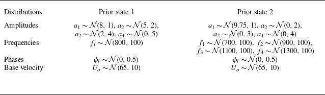
free parameters available in (4.1). The initial values imposed for the parameters at the very beginning of the DA run are important because they can lead to the convergence of the algorithm towards a local optimum, therefore reducing the potential accuracy of the DA tool (Asch et al. Reference Asch, Bocquet and Nodet2016). Considering the importance of this element for the analysis of turbulent flows, two prior states are investigated, whose features are reported in table 2.
Probabilistic distribution of the parameters describing the inlet boundary condition used as prior states for the DA parametric optimisation.

First, the prior state for each free coefficient is described using random Gaussian distributions, but the values are truncated to
 $\pm 2\sigma$
in order to avoid ill-conditioned problems. The distribution referred to as prior state 1 is selected to examine in detail the variability of the amplitude parameters. The latter directly controls the velocity levels of the inlet, therefore a high sensitivity to its variations is observed. For this reason, the distributions of the four parameters
 $a_i$
are deliberately chosen to be significantly different from one another. Similarly, the investigation using prior state 2 focuses on assessing the sensitivity of the optimisation to large variations in the examined frequencies, the distribution of which is given in table 2. In both cases, the parameters describing the phase and the base velocity are initially obtained using a Gaussian distribution centred around the true value imposed in the run LES-HF. Although the parameters are still optimised, this simplification has been intentionally chosen to focus on the investigation of the amplitude and frequency of the velocity fluctuations. Once the initial coefficients are determined for each ensemble member and for the two configurations, one can observe the behaviour of the inlet conditions during the forecast step simply by tracing the curves obtained by (4.1) and without any need to perform simulations. These diagrams are shown in figure 15. Figure 15(a,b) provide information about prior state 1, while figure 15(c,d) include results from prior state 2. In figure 15(a,c), one can see the inlet behaviour of LES-HF (in red), with the same condition initially prescribed for the ensemble members. Figure 15(b,d) do not include information on each simulation of the ensemble, but provide its mean (blue line) and its standard deviation (grey region). As expected, prior state 1 exhibits higher amplitude variations when compared with prior state 2. The latter, however, shows higher frequency dynamics. Finally, for every simulation of the ensemble, the initial velocity and pressure fields are taken from LES-LF for
 $t = 10 t_p$
.
Evolution of the normalised axial velocity inlet condition for (a,b) the distribution prior state 1 and (c,d) the distribution prior state 2. The red curve corresponds to the reference inlet condition used for LES-HF. The grey curves correspond to realisations for the ensemble members. The blue curve corresponds to the mean of the ensemble members. The grey area indicates the standard deviation.

As mentioned previously, data are sampled at
 $400$
sensors positioned in the physical domain for LES-HF. These sensors measure the instantaneous values for the three velocity components for a total of
 $1200$
observations for each analysis phase. The sensors are positioned in the jet area at the outlet of the intake duct, on the planes
 $y = 0$
and
 $z = 0$
presented in § 3.2. The selected positions are shown in figure 16 for reference. Data are observed for cycles
 $7$
–
 $10$
of LES-HF to eliminate effects associated with the initial conditions, providing a total of four cycles for analysis. To extend the time window for DA, the observation is restarted from the beginning of cycle
 $7$
after the last snapshot from cycle
 $10$
is used. It has been verified that these two instantaneous solutions remain similar, and in particular, that sensor data do not exhibit significant differences. This verification ensures that resampling the observation from cycle 7 does not introduce strong discontinuities in the flow field, preventing convergence issues in the algorithm.
Normalised velocity field of the run LES-HF for
 $t=9 t_p$
shown on two sections for
 $y=0$
and
 $z = 0$
. The red dots correspond to the
 $400$
sensors providing observation to calibrate the inlet condition. Sensors are mostly positioned in the jet area.

Finally, the DA strategy and the selected hyperparameters are discussed. The main feature of the HLEnKF is that multiple analyses are performed on smaller domains corresponding to a sufficiently large volume around each sensor. The size of each domain, further explained in § 5, is approximately
 ${3.4\times 10^{-3}}\,\textrm {m}$
. Considering that the domains are clustered in four main regions, and they are close together, some regions are overlapping. This overlap is not important for the present DA analysis because no state update is performed, and the only target is the optimisation of the inlet boundary conditions. To this purpose, the optimised parameters obtained by each local EnKF are averaged before the updated values are sent back to the ensemble members, updating the inlet.
The size of the state matrix
 $\boldsymbol{\mathcal{U}}$
is
 $[N_{\textit{ext}}, N_e]$
, where
 $N_e=35$
is the number of ensemble members, and
 $N_{\textit{ext}} = N + N_{\gamma }$
represents the total number of degrees of freedom considered for each analysis phase. Here,
 $N$
characterises the features of the flow field in the local region of the analysis, and usually
 $N = 3 \, n_{cells}$
. Indeed, the local HLEnKF procedure considers all three components of the velocity field measured at each grid element. However, since no state estimation is performed in this case, and the flow field information is already incorporated in the terms
 $s_i$
, the value of
 $N$
is set to zero. Consequently,
 $N_{\textit{ext}}$
and
 $N_\gamma$
are both equal to
 $13$
, which is the number of free parameters optimised by the DA procedure.
Scheme illustrating the time window required to advect downstream the updated inlet information to the sensors. On average, this time window is
 $\gt t_p$
.

The time frequency of the analysis phases is particularly important because once the parametric description of the inlet is updated via the DA procedure, sufficient time must be allowed for the signal to propagate and influence the observation region before conducting a new analysis. This time can be estimated taking into account the oscillating features of the flow imposed at the inlet. An algebraic estimation is obtained by
 $t_A^{\textit{inletDA}} = (L_e + L_{vh})/u_b \approx {1.75\times {10}^{-3}}\,{\textrm{s}} = 1.4 t_p \gt t_p = {1.25\times {10}^{-3}}\,{\textrm{s}}$
when considering the advection by the mean velocity
 $u_b$
. Therefore, differences are observed during the cycle, and the time window can actually be smaller than
 $t_p$
when the velocity at the inlet is close to its maximum. A visual representation is provided in figure 17 for a qualitative description. Clearly, analysis over a short time span would operate using the wrong correlation between the observed results at sensors and the parametric description of the inlet, potentially leading to the divergence of the filter. One possible solution to avoid this constraint is to rely on an ensemble Kalman smoother (Evensen & Van Leeuwen Reference Evensen and Van Leeuwen2000) algorithm, which enables optimisation over larger time windows that include multiple analyses. However, computational and storage costs for this case would be prohibitive. The preliminary tests performed show that in this case, the very first analysis phase is critical. The following DA optimisations are progressively less critical as the offset between the data observed at the sensors and the parametric description of the inlet reduces as the free parameters reach convergence. After the first cycle, which usually allows us to obtain an adequate value of optimisation, the update can be performed over shorter periods as corrections to the parameters are going to be smaller, and the optimisation exhibits good features of robustness. Keeping a large analysis window would probably produce the same final result, but more analysis phases would be required (thus observation over an increased number of cycles). Therefore, the following DA has been performed. Once the procedure starts, the first forecast phase runs for a duration
 $t_{f,1}=2.2t_p$
, allowing the flow field obtained with the initial inlet conditions to propagate downstream for all 35 ensemble members. After this first analysis phase, the length of the forecast phase is reduced to
 $t_{f}=0.2 t_p$
, i.e. five analysis steps are performed for each cycle. The DA runs are performed for a total time
 $12t_p$
, for a total of
 $50$
analysis steps.
The last set of hyperparameters to be discussed is the confidence level imposed for the observations and for the model. The measurement error covariance matrix
 $\boldsymbol{R}$
in (2.20) is diagonal and expressed as
 $\boldsymbol{R} = \sigma _m^2\boldsymbol{I}$
, where
 $\sigma _m$
quantifies the uncertainty of the measurements. A multiplicative uncertainty of
 $17.5\,\%$
is applied to the values of each observation during the first three inferred cycles. Thereafter,
 $\sigma _m = 5\,\%$
. This choice has been made to obtain a robust convergence of the parametric optimisation. Stochastic inflation (see § 2.2.1) is used to increase the variance of the parametric description during the calculation. Recall that inflation is an excellent tool to avoid the collapse of the variance of optimised parameters. This phenomenon, which is common using the classical formulation of the EnKF, can preclude the identification of efficient regions in the parameter’s space once a local optimum is identified. Low values for inflation value are hence used after the first inferred cycle, i.e.
 $\lambda = 0.5\,\%$
. After the ninth cycle, the coefficient controlling the multiplicative inflation is again lowered to
 $\lambda = 0.375\,\%$
.
4.2. Results obtained for the DA parametric optimisation
The results of the calibration of the free parameters of the inlet boundary condition for prior state 1 and prior state 2 are discussed in this subsection. Figures 18 and 19 show the velocity field for the ensemble realisations measured at the sensors positioned in the intake duct (shown in figure 9), which were used to study the features of the LES-HF run. Figures 18(a,d) and 19(a,d) correspond to the sensor located at the inlet boundary condition. Figures 18(b,e) and 19(b,e), and figures 18(c, f) and 19(c, f), correspond to the sensors located in the middle of the intake pipe and in the proximity of the valve region, respectively. Comparing the present results with those reported in figure 15 for the non-optimised inlet conditions, one can see that the modifications performed by the HLEnKF are visible from the second or third cycle, as expected. A slight delay can be observed for the two sensors in the middle and at the end of the intake pipe, caused by the time required to transport the updated solution downstream. For both DA runs, the optimisation procedure provides an adequate reconstruction of the flow features. In particular, the variance of the ensemble reaches a converged behaviour at approximately cycle 5 or 6. One interesting point here is that despite significant differences in the initial conditions for the two prior states investigated, the DA algorithm successfully reconstructs the global dynamics, even when relying on localised instantaneous flow observations. This result highlights the robustness of the algorithm to variations of the prior conditions.
Evolution of the axial velocity for the distribution prior state 1. Red curve: LES-HF. Grey curves: DA ensemble members. Blue curve: average of ensemble members. Shaded area: standard deviation from the mean. Data are sampled from sensors at (a,d)
 $x=0$
, (b,e)
 $x=0.046$
and (c,f)
 $x=0.092$
shown in figure 9.

One interesting feature that is observed in both runs is that the amplitude of the velocity signal obtained via DA (blue line) is very similar to the one sampled for LES-HF for the sensor downstream (figures 18(c, f) and 19(c, f)). Moving upstream, one can see that the signal follows the same dynamics, but it is, on average, lower. This is particularly visible at the inlet (figures 18(a,d) and 19(a,d)) for prior state 2. This result is justified by the numerical and modelling errors observed in LES-LF using a coarse grid. One consequence of these errors is that the velocity at the end of the intake pipe is higher than for the case LES-HF. Therefore, one can see that the DA optimisation here decreases the velocity at the inlet in order to match the observed velocity in the valve region. The DA calibration of the inlet compensates for the effects of the numerical errors over the flow prediction in the intake pipe, so that the predictions in the valve region between model and observation are the same.
Evolution of the axial velocity for the distribution prior state 2. Red curve: LES-HF. Grey curves: DA ensemble members. Blue curve: average of ensemble members. Shaded area: standard deviation from the mean. Data are sampled from sensors at (a,d)
 $x=0$
, (b,e)
 $x=0.046$
and (c, f)
 $x=0.092$
shown in figure 9.

The same conclusions can be drawn via the investigation of the time evolution of the ensemble average of the free parameters describing the inlet velocity, which are shown in figure 20 for both DA runs. The time evolution of their standard deviation is also reported in Appendix A. The base velocity in figure 20(a,e), the amplitudes in figure 20(b, f) and the frequencies in figure 20(c,g) are adimensionalised by the reference values used for LES-HF. The base velocity seems to converge to a value
 $2$
–
 $4\,\%$
lower than the reference value for both DA runs. This result supports previous discussion about the compensation of numerical and modelling errors due to the usage of the coarse grid. The amplitude parameters are now investigated. A perfect DA calibration would have here provided the convergence of three amplitude parameters to
 $0$
, while the last one would have converged to the value imposed for the LES-HF run. Differences are observed here for the cases prior states 1 and 2. For the latter, the amplitude coefficients actually converge to the desired values fairly quickly, with tolerance
 $\approx 5\,\%$
, and they exhibit very mild variations in time. It is, however, important to stress that the amplitude parameters here converge to the mean value of the Gaussian distribution imposed as initial condition. For the case prior state 1, a mild evolution is observed in particular for the parameters
 $a_2$
and
 $a_3$
, which appear to compensate for each other (see figure 20
b). Therefore, the DA algorithm yields two distinct optimisation strategies. For prior state 1, mild variations in amplitudes are observed, which are compensated by occasionally significant changes in phase, frequencies and base velocity. For the latter two, one could even argue that no convergence is reached, as the algorithm continues to adjust these quantities over time to compensate for the inaccurate convergence observed in the amplitude parameters. On the other hand, the better guess in terms of initial estimation of the amplitude coefficients for prior state 2 provides a rapid convergence towards expected values for all the parameters at play; see in particular the blue lines for the frequency and the phase in figures 20(g) and 20(h).
Evolution of the parameters describing the inlet condition during the assimilation procedure for the distribution (a–d) prior state 1 and (e–h) prior state 2. Blue: sine function 1. Yellow: sine function 2. Green: sine function 3. Red: sine function 4.

Time evolution of the streamwise velocity imposed at the inlet. Results are shown for (a–c) the distribution prior state 1 and (d–f) the distribution prior state 2. The red curve represents the inlet’s velocity imposed on the run LES-HF, and the blue curve is obtained using the coefficients obtained with the DA optimisation at (a,d)
 $t=6t_p$
, (b,e)
 $9t_p$
and (c,f)
 $12t_p$
.

The parametric description of the DA run is now sampled and investigated for some specific analysis phases. To this purpose, the inlet parameters sampled at times
 $t = 6t_p$
,
 $t = 9t_p$
and
 $t=12t_p$
are considered to be frozen, and they are used to visualise the resulting inlet behaviour over a longer time window. The plot of these inlet functions is shown in figure 21. Figure 21(a–c) show the inlet evolution calculated with the parameters optimised for prior state 1, while figure 21(d–f) include the same plot for prior state 2. In both cases, the plot is performed for 100 cycles, enabling to observe the time evolution of the signal. These results confirm previous discussion about the optimisation of the coefficients. For prior state 1, the inaccurate estimation of the amplitude coefficients requires time-dependent variations of the other free parameters to maintain a low discrepancy in time with the LES-HF observations. On the other hand, for prior state 2, where the initial amplitude guess is more accurate, the optimisation rapidly converges to a parametric configuration that effectively reproduces the inlet characteristic of the reference simulation. The clear identification of why the two prior states lead to different attractors is challenging in this case because of the very large number of elements affecting the instantaneous evolution of the LES solution. However, one can see that for prior state 2, the selected mean values for the frequencies and their variances overlap pretty well the target frequency of the inlet for the reference simulation. This is not the case for the amplitudes for prior state 1, where prior values (in terms of average and variability due to the variance) individually underpredict the targeted amplitude value. Therefore, optimisation for prior state 1 is more complex because the targeted value may be outside the space covered by the initial state distribution of the ensemble members. Because of the unsteady features of the flow, one can conjecture that the EnKF does not manage to clearly identify the true attractor; however, it is able to adapt in time its prediction in order to match instantaneous measurements (and accounting for the provided level of confidence/uncertainty on such data).
In summary, the application of the HLEnKF algorithm successfully achieves a robust calibration of the inlet conditions for the DA ensemble members running on coarse grids, using instantaneous velocity samples from the high-fidelity LES-HF simulation as observations. However, this efficient calibration is obtained via a precise analysis of optimised time windows between consecutive analysis phases, including knowledge of the characteristic times of the flow. Considering that such information is rarely available, the present analysis shows the potential to perform DA optimisation for turbulent flows, as well as the challenges and difficulties that have to be considered in this process. Among the latter, it is demonstrated that the choice of different prior states strongly affects the results of the optimisation. On the one hand, the results of the DA optimisation starting from prior state 2 rapidly converge towards the expected coefficients. One could also see that the resulting set of inlet parameters takes into account the numerical and modelling errors developing in the intake pipe, in order to minimise the discrepancy between model runs and observations. On the other hand, the algorithm fails to converge to the expected parameter values when using prior state 1. To address this issue, the DA algorithm adjusts the parameters at each analysis phase to enhance the quality of the prediction. Despite the differing outcomes in parameter optimisation for the two DA runs, both successfully capture a convincing representation of the inlet characteristics. From this perspective, the HLEnKF proves effective in achieving robust parametric optimisation for both prior configurations used, providing interesting perspectives for the reconstruction of realistic unsteady boundary conditions necessary in future studies using digital twins.
5. Flow synchronisation using DA
The results presented in § 4 showed that the HLEnKF performs an adequate calibration of the free parameters of an unsteady inlet condition when using observations from sensors. Therefore, the DA optimisation acts so that the flow dynamics obtained for the ensemble members is similar to that of the simulation from which the observation was sampled. The attention is now focused on the capability of the DA algorithm to synchronise the instantaneous behaviour of the flow field predicted by the numerical models with the observation. This point is challenging for turbulent flows, considering that two identical configurations have the same statistical behaviour but may have very different instantaneous flow fields. Efficient synchronisation may unlock advancement in multiple research fields dealing with engineering. In such applications, the synchronisation of complete numerical models with localised data measured at sensors (such as e.g. in a digital twin architecture) provides a tool for the analysis and potential anticipation of certain extreme conditions and events that could lead to a decrease in the efficiency of the physical system, or harm its integrity. Two objectives are targeted in this section. The first deals with the assessment of the synchronisation capabilities of the HLEnKF when sparse observation is provided. The second objective is to investigate how the DA state update performing the synchronisation affects the statistical moments of the flow, and in particular its modal energy distribution. This second point is essential to validate the capabilities of the DA algorithm to improve the physical accuracy of the model when limited measurements are provided.
5.1. Set-up details
The starting point of this analysis is the DA calibration procedure performed with prior state 2. The inferred configuration obtained via the calibration of the inlet parameters for the latter will be referred to as LES-PE2 from now on. Recall that this DA run was performed for a total time
 $t = 12t_p$
. The 35 ensemble members show very similar but not identical parametric descriptions of the inlet due to the inflation applied to the system. Therefore, their instantaneous physical fields for
 $t=12t_p$
are not identical. The analysis using DA state estimation to evaluate the synchronisation properties is now performed starting from this set-up, and it is run for one complete cycle, thus ending at
 $t=13t_p$
. Considering that the DA analysis period is only one
 $t_p$
, the limitations in terms of time window between successive DA analyses are no longer relevant, and a maximum of 1250 analyses can be performed over the period of investigation, which corresponds to the sampling rate of LES-HF. It is important to recall that the observation from the LES-HF run was taken from cycles 7–10, and that the observation was reused once the set was over. Considering that the DA analysis started at the end of the second cycle for the run LES-PE2, this means that data from the ninth cycle of the run LES-HF are used as observations in the time window
 $t \in [12t_p, 13t_p]$
. The LES-HF velocity field for the time
 $t=9t_p$
is shown in figure 11. The sensors used in these investigations are now described. The set previously used for DA calibration in § 4 is now expanded, including additional sparsely distributed sensors on the plane
 $x={0.124}\,\textrm {m}$
(see figure 12). A total of
 $582$
new sensors are included. This new sensor set, called the SE-set (state estimation set) is shown in figure 22. A sensitivity analysis using a second sensor set, SE-set2, is provided in Appendix B, but this is not included here for the sake of conciseness.
Velocity field of the run LES-HF for
 $t=9 t_p$
shown on two sections for
 $z=0$
and
 $x = {0.124}\,\textrm {m}$
. The red dots correspond to the
 $582$
observation sensors selected to perform the state estimation in the synchronisation procedure (SE-set).

The size of the state matrix
 $\boldsymbol{\mathcal{U}}$
is now discussed. As previously stated in § 4, its size is
 $N = 3 \, n_{cells}$
if no parametric optimisation is performed (
 $N_\gamma =0$
). However, the number of elements
 $n_{cells}$
changes for each local EnKF performed, and it is a function of the volume of the region as well as of the local grid refinement. The volume is here considered to be spherical, and the diameter is selected with respect to the covariance localisation length used for the DA analysis. For this test case, which exhibits turbulent features, the localisation length is related to the integral length scale
 $\mathcal{L}$
. This choice appears to be the most logical, as the correlation of the velocity field in turbulent flows rapidly decays for distances that are larger than
 $\mathcal{L}$
. Therefore, it is an appropriate length scale for covariance localisation. The integral length scale calculated using the velocity field from LES-HF exhibits an average value
 $\mathcal{L} \approx {1.7\times {10}^{-3}}\,\textrm {m}$
. To take into account the distance between sensors, and in order to reduce superpositions of the zones where different realisations of the HLEnKF are performed, the diameter of the localised regions for the HLEnKF is selected to be
 ${2.5\times {10}^{-3}}\,\textrm {m}$
. Moreover, in order to obtain a DA state update of
 $\approx 1\,\%$
in the proximity of the external surface of each volume for the HLEnKF, the parameter
 $l$
in (2.26) is set to
 $l={4.1\times {10}^{-4}}{}$
. This leads to
 $ \approx 63 \, 000$
grid elements, or
 $N \approx 189 \, 000$
degrees of freedom for each of the
 $134$
realisations of the HLEnKF. The number of regions does not match the total number of sensors, because some of them were clustered due to physical proximity. The number of elements in every region may exhibit variations depending on the local grid refinement. It is, however, important to stress that performing
 $134$
DA procedures for the selected volumes around sensors is significantly less computationally expensive than performing one single EnKF using data from eight million grid elements.
Table 3 summarises the features of the runs performed to evaluate the accuracy of the DA state estimation and synchronisation. For all simulations, the time window between successive analyses is constant. However, the sensitivity to the length of such a time window and its impact on the predictive capabilities of the DA algorithm is investigated. To this purpose, three runs are performed using the SE-set. The first run used the shortest possible time window, corresponding to the sampling period of LES-HF. This time window is
 $t_{\textit{DA}} = 10\varDelta _t = {1\times {10}^{-6}}\,{\textrm{s}}$
. The frequency at which DA is performed is therefore
 ${1000}\,\textrm {kHz}$
in this case. The second configuration uses a time window
 $t_{\textit{DA}} = 50\varDelta _t$
, and for the third one,
 $t_{\textit{DA}} = 250\varDelta _t$
. The corresponding assimilation frequencies are then
 ${200}\,\textrm {kHz}$
and
 ${40}\,\textrm {kHz}$
. These runs are referred to as LES-TW10, LES-TW50 and LES-TW250, respectively. We stress that when compared to the characteristic frequency scale of engine flows, the number of time samples per period used here could typically be obtained by using optical techniques such as high-speed particle image velocimetry (Voisine et al. Reference Voisine, Thomas, Borée and Rey2011; Leite et al. Reference Leite, Brequigny, Borée and Foucher2024) used currently in optical engines. Acquisition frequencies for particle image velocimetry measurements are typically in the range
 ${1}$
–
 ${10}\,\textrm {kHz}$
(Galmiche et al. Reference Galmiche, Mazellier, Halter and Foucher2014). However, the frequency of the velocity time signal imposed at the inlet for the run LES-HF is also
 $\approx 6$
times higher than the characteristic frequencies observed in internal combustion engines. Therefore, one can see that the second configuration investigated falls into a range of number of time samples per physical oscillation of the flow that is observed in experiments. These three runs are compared with the results obtained from the run LES-PE2, which is also continued for one cycle using the same analysis time windows used for calibration (
 $2500 \varDelta _t$
).
Summary of the runs performed to investigate DA state estimation for field synchronisation, compared with the run LES-PE2 (TW indicates time window, and PE2 indicates parameter estimation run 2).

The DA capabilities to perform efficient synchronisation are evaluated via the calculation of a root mean square error
 $\varPhi$
evaluated at each analysis phase
 $k$
:
 \begin{equation} \varPhi (k) = \sqrt {\sum _{j=1}^{N_o}{(\langle \boldsymbol{s}_{\!j,k} \rangle -\boldsymbol{\alpha }_{j,k})^2}}\Biggl /N_o, \end{equation}
where
 $\langle \boldsymbol{s}_{\!j,k} \rangle$
is the mean of all the velocity values calculated by the ensemble members at the coordinates of the sensors,
 $\boldsymbol{\alpha }_{j,k}$
are the sampled observations, and
 $N_o$
is the number of sensors. This indicator allows evaluating the global discrepancy between the assimilated velocity field and the high-fidelity reference at the sensors. The calculation of
 $\varPhi (k)$
is carried out considering the 582 sensors for the three configurations LES-TW10, LES-TW50 and LES-TW250. For the first one, two levels of confidence in the observations are considered (uncertainty levels
 $5\,\%$
and
 $20\,\%$
) as well as two levels for the inflation (
 $0\,\%$
and
 $5\,\%$
). The evolution of
 $\varPhi$
for these calculations is shown in figure 23. This indicator varies in time for all the runs, exhibiting values included in the range
 $[0.2, 1.2]$
. The black curve represents the evolution of the error for the configuration without any state estimation LES-PE2. It is representative of the variability of the 35 simulations of the ensemble. The red and orange curves correspond to the runs LES-TW250 and LES-TW50, which are performed using a confidence level for the observations
 $\sigma _m = 5\,\%$
. For the former, the values of
 $\varPhi$
are extremely similar to those observed for the case LES-PE2, which suggests that the DA time window is too large to obtain a permanent signature on the instantaneous structural organisation of the flow. On the other hand, results for the run LES-TW50 show that the discrepancy is globally reduced at each time step over the cycle investigated. A similar behaviour is observed for
 $\varPhi$
for the four realisations of the LES-TW10 run. The green curves (which superpose on each other) are obtained with confidence level
 $20\,\%$
in the observations, while the blue curves are obtained with confidence level
 $5\,\%$
. One can see that variations in the values selected for the inflation do not strongly affect the results. Generally speaking, the best runs for the configuration LES-TW10 exhibit an error reduction of at least
 $60\,\%$
at all times when compared with the LES-PE2 run. This result shows the sensitivity of the noise affecting the observations in the DA procedure. While this parameter is governed by the quality of the acquisition system, these results indicate how this parameter can be adapted to improve the global synchronisation of the flow. On the other hand, the low sensitivity to inflation can be justified by two factors. First, a good degree of initial variability of the flow field is granted by the selected prior distribution. Second, the problem of variance collapse observed for classical EnKF algorithms is not as strong for the HLEnKF, due to the physical localisation affecting the state update.
Evolution of the root mean square error
 $\varPhi$
over the time of investigation. Black curve: run LES-PE2. Red curve: run LES-TW250 with
 $5\,\%$
confidence in the observation and without inflation. Orange curve: run LES-TW50 with
 $5\,\%$
confidence in the observation and without inflation. Green curves: run LES-TW10 with
 $20\,\%$
confidence in the observation and inflation equal to (light green)
 $0\,\%$
and (dark green)
 $5\,\%$
. Blue curves: run LES-TW10 with
 $5\,\%$
confidence in the observation and inflation equal to (light blue)
 $0\,\%$
and (dark blue)
 $5\,\%$
.

5.2. Synchronisation capabilities
The study of the root mean square error
 $\varPhi$
using different hyperparameters showed that a confidence level in the observations of
 $5\,\%$
and zero inflation provided the most accurate results. However, this evaluation is performed using a global indicator. The local synchronisation capabilities for the runs performed are now investigated. To this purpose, three different sensors providing observation are monitored to study the evolution of the instantaneous velocities obtained via DA and compare them with the available high-fidelity data. These sensors, which are summarised in table 4, are located on the plane
 $x={0.124}\,\textrm {m}$
; see figure 24. Sensors 1 and 2 are located in the proximity of the valve outlet jet on opposite regions of the plane, while sensor 3 is slightly off-centre in a zone with higher shear.
Sensors used to assess the accuracy of the synchronisation between the DA prediction and the observation.

Sensors used to assess the accuracy of the synchronisation between the DA prediction and the observation.

Synchronisation of the axial component of the velocity
 $u_x$
between DA model representation and observations. Results are shown for (rows) different DA runs and (columns) at different sensors. The blue curves represent the observation. The black lines show the average prediction for the DA ensemble. The red lines provide results for member 27 of the ensemble without performing DA. The green lines provide results for member 27 of the ensemble when using DA.

Figure 25 shows the axial component of the velocity field for the runs performed at the three sensors investigated. The evolution of the instantaneous velocity component
 $u_x$
(normalised by the reference bulk velocity
 $u_b$
) is shown in blue for LES-HF, i.e. the one from which the observation is sampled. The results from the ensemble members of the DA procedure are shown in black (ensemble mean). Shaded areas around the blue and black curves correspond to the standard deviation of the measured velocity field. The red and green curves show the velocity evolution for member 27 of the database. The red curve corresponds to a run where the simulation is forecast in time without any DA correction, while the green line corresponds to the actual velocity profile when state estimation is performed. Results are now commented on for each of the DA runs performed. Figure 25(a–c) correspond to the run LES-PE2, which does not include state estimation but was calibrated via the inlet inference in § 4. As observed previously, the level of variance of the ensemble indicated by the shaded grey areas is relatively high. This is due to the variability imposed for the ensemble velocity fields via inflation. The analysis of the green lines shows high instantaneous variations that are similar to the case without any DA, illustrated by the red curve. Neither of the two velocity profiles appears to synchronise with the blue curve representing the observation for any of the three sensors. Therefore, no synchronisation is observed for the LES-PE2 case.
Figures 25(d–f), 25(g–i) and 25(j–l) present results for runs LES-TW250, LES-TW50 and LES-TW10, respectively. Here, a synchronisation of the flow field is observed progressively. Improved flow reconstruction is obtained for shorter time windows between DA analyses. One can also see that a more accurate synchronisation comes here with a significant reduction of the variance of the ensemble prediction. This point is clear comparing results from figures 25(d–f) and 25(j–l). The grey areas show a fast reduction of the ensemble variance after the first analysis step. However, contrary to the classical EnKF behaviour, this reduction does not get close to zero values, but it reaches values close to the confidence level set for the observations. This point can be observed via the analysis of the superposing blue and grey areas. On the other hand, when analyses are too far away in time, state updates tend to be too important due to the large discrepancy between model prediction and observation, which is here due to the cumulative numerical errors in time. Because of the strongly nonlinear features of the flow, these corrections may lead to non-physical oscillations of the flow. This trend is visible for the results from the run LES-TW250 in figure 25(d–f). The run LES-TW50 shows satisfactory results with an adequate synchronisation capability. The best synchronisation features are achieved by the LES-TW10 run. For all three sensors considered, the ensemble mean almost perfectly coincides with the observation. The use of the HLEnKF shows good efficacy in synchronising the velocity field of the ensemble members with the high-fidelity observation. This result opens perspectives of local flow synchronisation while respecting global flow features, which is granted by the resolution of the Navier–Stokes equations performed in the ensemble runs. This point is now investigated further via the analysis of the statistical behaviour of the flow on the plane
 $x={0.124}\,\textrm {m}$
.
The jet moving outside the valve directly crosses this plane, then the flow is redirected by the cylinder wall to create a recirculation region, which forces the flow to cross again the investigated plane. The investigation of the modal energy distribution of the flow on this plane can therefore provide relevant information about the global accuracy of the HLEnKF. This investigation is complementary to the study of the local synchronisation features in correspondence with the DA sensors.
The instantaneous axial velocity field
 $u_x$
sampled from the LES-HF reference simulation for the time
 $t=9t_p$
is shown in figure 26. A Fourier transform of this field in the azimuthal direction is performed to investigate the characteristic modes representing the distribution of the kinetic energy. To do this, available data are first cast in the same polar coordinates for all the configurations (see figure 26
b). The discrete Fourier transform of the velocity for each radius available can be expressed as
 \begin{equation} \hat {u}_m(r) = \sum ^{N_{\theta }-1}_{n_\theta =0}u_{n_{\theta }}(r) \exp({-2\pi i m n_\theta /N_{\theta }}), \end{equation}
with
 $n_\theta = 0,1,2, \ldots ,N_{\theta -1}$
corresponding to the azimuthal discretisation. The modal energy distribution obtained for the DA runs is now compared with the results obtained for the LES-HF reference. It is obtained by calculating the power spectrum of each mode
 $P^m_s(r)=|\hat {u}_m(r)|^2$
.
Normalised axial velocity
 $u_x / u_b$
for the run LES-HF. Data sampled on the plane
 $x = {0.124}\,\textrm {m}$
: (a) measurements at sensors, (b) transformation in polar coordinates.

Modes of the azimuthal Fourier transform of the fluctuation of the axial velocity
 $u_x-\overline {u_x}$
at time
 $t=13t_p$
on the plane
 $x = {0.124}\,\textrm {m}$
. Results are shown for
 $r/R \in [0.35, 0.95]$
, which represents the jet area and the recirculation region. The images are coloured according to the spectral power
 $P_s$
normalised by the maximum power value
 $\max (P_s)$
for each case.

Figure 27 shows the distribution of the first
 $11$
modes of the Fourier transform of the axial velocity. The energy carried by the remaining modes is not significant. The azimuthal mean (mode 0)
 $u_x-\overline {u_x}$
is here excluded to investigate the features of the fluctuating field. Results are shown for the LES-HF reference simulation and for simulation 27 of the ensemble for each DA run. In particular, the results for prior state 2, for the LES-PE2, LES-TW50 and LES-TW10 configurations are reported. The images are coloured according to the spectral power
 $P_s$
normalised by the maximum power value
 $\max (P_s)$
for each case. These power spectra provide the kinetic energy (per radians) carried by each Fourier mode. The distribution for LES-HF presents three main modes: mode 1 contains a large amount of energy in the recirculation region of the flow (
 $r/R \approx 0.9$
), while modes 6 and 10 present large amounts of energy in the jet shear region (
 $r/R \approx 0.5$
). Modes 2 and 3 also provide important contributions in these two regions. The prior state 2 simulation shows a very high energy level in the shear region (
 $r/R \approx 0.45)$
for mode 2 and partially mode 1, but the energy content for other modes is weak. In particular, the energy distribution observed in the recirculation region is very low when compared with the results from the LES-HF run. The calibration of the inlet condition for the LES-PE2 run strongly affects the energy distribution. A very high level of energy is now observed in the recirculation region for several modes. Results for the DA runs LES-TW50 and LES-TW10, which are shown in figures 27(d) and 27(e), exhibit the closest match to the predicted modal distribution of the reference simulation. The energy distribution for both DA runs exhibits a clear multi-modal behaviour in the shear region, while modes 1, 2 and 4 are dominant in the recirculation region. This last result is promising, as DA sensors are not close to the recirculation region. Therefore, one can see that the usage of a CFD model based on Navier–Stokes equations is able to correctly propagate a local state update to obtain an improved global prediction. These findings are in line with previous results found by Meldi & Poux (Reference Meldi and Poux2017), who observed similar results for DA applications using scale-resolved CFD.
Modes of the azimuthal Fourier transform of the velocity component
 $u_y$
at time
 $t=13t_p$
on the plane
 $x = {0.124}\,\textrm {m}$
. Results are shown for
 $r/R \in [0.35, 0.95]$
, which represents the jet area and the recirculation region. The images are coloured according to the spectral power
 $P_s$
normalised by the maximum power value
 $\max (P_s)$
for each case.

Finally, the component
 $u_y$
of the velocity field is studied. Considering the symmetric behaviour of the test case,
 $u_z$
is not investigated, as the results are statistically the same. Figure 28 presents the distribution of the first
 $11$
modes for the Fourier transform of
 $u_y$
. In this case, mode 1 is predominant over all the other modes. The energy is concentrated in the shear region, where the jet has not yet impacted the cylinder wall. This strong energy concentration is observed from
 $r/R = 0.45$
to
 $r/R = 0.65$
for the reference LES-HF. For prior state 2, the distribution is smaller, and a high density of energy is observed for
 $r/R = 0.45$
and
 $r/R = 0.55$
. The results for the run LES-PE2 show a significant overprediction of the energy content for modes 1 and 3 in the proximity of the recirculation region, showing again a significant discrepancy. The runs LES-TW50 and LES-TW10 also show a high energy concentration of energy for mode 1 in the recirculation region, but the results are in adequate agreement with the reference simulation.
Comparisons of instantaneous fields for the reference run of § 3.2, prior run of § 4, calibrated inlet run of § 4 and synchronised flow run of § 5. The velocity magnitude is shown on a section for
 $z=0$
, and normalised by the reference velocity
 $u_b$
. The normalised pressure
 $p/p_{\boldsymbol{atm}}$
is shown on the surface of the valve guide.

In summary, the investigation of the energy distribution using a discrete Fourier transform shows that the HLEnKF is able to provide an accurate prediction of the statistics of the flow field. Despite the local behaviour of the state update, the distribution of the kinetic energy exhibits an accurate behaviour even far from the assimilation regions. The energy distribution of the non-axial component of the velocity, however, shows differences between all the studied configurations, despite the excellent synchronisation of all the velocity components. A qualitative comparison of the velocity fields for the plane
 $z=0$
is shown in figure 29. It illustrates in particular the phase shift of prior state 2 compared to the calibrated LES-PE2 configuration. Furthermore, LES-TW10 presents topological improvements of the velocity structures without, however, recreating the characteristic ‘clamp’ shape shown on the LES-HF reference simulation. The pressure distributions in the intake region are different principally because of the model error. The usage of a coarser grid in LES is responsible for several sources of error that interact with each other. These nonlinear interactions affect the calibration of the inlet, as the Kalman filter targets a minimisation of the discrepancy between model and observation in the proximity of the sensor. The discrepancies observed for the pressure field, which is calculated by the CFD code, are a result of this bias in the velocity field. This is not necessarily a negative point, as the predicted pressure is consistent with the velocity field predicted by the ensemble members. In this scenario, a pressure field similar to the reference run would then violate the conservation of physical laws. If the obtention of an accurate pressure field is a target objective, then one could envision applications using a DA smoother, which could help to reduce these discrepancies. However, this potential improvement would probably require an increase in computational resources due to the need to store additional solutions.
The topological improvements – the synchronisation of the velocities in the inferred zones as well as the improved prediction of the energy distribution of the flow – highlight the potential of highly localised sequential DA in the digital twin paradigm. A specific point of interest for future investigations regards the predictions and tracking of extreme events, which is usually challenging for scale-resolving simulations. These kinds of events, described by rapid and significant variations of the topology of the flow, are usually provoked by minimal variations in some upstream conditions, which are amplified by the strongly nonlinear, multiscale nature of turbulence. The possibility to create a numerical replica of these events is critical to predict key quantities such as turbulent energy production and dissipation, and their influence over the flow features in the following turnover times.
6. Conclusion
A data assimilation (DA) tool based on the ensemble Kalman filter (EnKF) has been used to augment scale-resolving numerical simulations. The analysis, which combined ensemble numerical runs using LES and high-fidelity data available on local sensors, has been performed for the investigation of the flow rig test case. The application of DA techniques to such a complex case, in terms of multiscale interactions and of degrees of freedom investigated, was possible thanks to the development of the HLEnKF technique and its implementation in the online library CONES. The investigation performed for this test case targeted two main objectives, which are (i) the calibration of the free parameters driving an unsteady inlet condition, and (ii) the efficient synchronisation of the flow field predicted by the LES model with the observation.
The DA calibration was performed twice, changing the initial values and variability of different parameters for the two prior states selected for investigation. In both cases, the HLEnKF showed a satisfactory calibration for scale-resolving turbulent conditions. However, the usage of different prior states created different attractors for the parametric configuration, highlighting the difficulties in the optimisation of such complex, nonlinear systems.
The HLEnKF state estimation was able to provide a local synchronisation of the inferred velocity fields with the observed data. However, it was observed that the frequency of DA analysis is a critical parameter here, and that if the time period between successive analyses is not of the same order of magnitude as the physical turnover time, then synchronisation is not reached. The study of the Fourier modes of the velocity fluctuation provided additional information on the quality of the reconstruction of the velocity field. Although unchanged for the
 $u_y$
and
 $u_z$
components of the velocity field, the modal distribution for the axial component
 $u_x$
was improved by the DA algorithm. A lower discrepancy with the reference data was also visible in the recirculation zone. No direct DA state update was performed in this region, but the advection of the flow from zones where the HLEnKF was performed had a positive effect on the accuracy of the solver.
This work permitted us to highlight the potential of such DA techniques for the investigation of turbulent flows using scale-resolving techniques, as well as to identify the challenging aspects to be faced in the near future to obtain robust predictive tools. Among the positive points, the potential for the integration of sequential DA in the digital twin paradigm is the most exciting. In fact, the reconstruction of unsteady boundary conditions and the synchronisation of the digital instantaneous flow field with the observed phenomenon are essential steps to envision a realistic application of the digital twin paradigm. The field of applications may include internal as well as external flows present in transport engineering, air quality prediction, energy harvesting and medical-pharmaceutical studies. Future advancement of these tools by the team targets applications to test cases of industrial interest. In particular, the usage of observation from experiments for complex cases will allow us to assess more clearly the potential and limitations of these techniques for realistic applications.
Acknowledgements
L.V. acknowledges the support of CERFACS during the editing and proofreading of this paper.
Funding
This work was supported by the French National Research Agency (ANR) to the ANR-20-CE05-0007 ALEKCIA project (https://www.ifpenergiesnouvelles.fr/alekcia). This work was also granted access to the HPC resources of TGCC under allocation no. A0162B10763 from the GENCI (Grand Equipement National de Calcul Intensif) eDARI programme.
Declaration of interests
The authors report no conflict of interest.
Appendix A. Standard deviation of the parameters considered for the calibration of the inlet boundary condition
Figure 30 shows the time evolution of the standard deviation of the parameters for the optimisations of the parametric description of the inlet performed in § 4 from prior states 1 and 2. The evolution of this quantity is representative of the variance collapse observed for the ensemble members of the EnKF. Because the multiple local parameter estimations are averaged within the HLEnKF algorithm, variance collapse is smaller when compared to a classical non-localised EnKF. This positive aspect is useful to preserve a suitable level of variance during the optimisation of the parameter, therefore requiring lower levels of artificial inflation. In particular, the value reached for all the parameters investigated corresponds to the variance rate imposed via the stochastic parametric inflation
 $0.5\,\%$
and then
 $0.0375\,\%$
used during the DA procedure. Comparisons in terms of accuracy and variance of the parameters between the classical implementation of the EnKF and the one used in this paper are further analysed in the Appendix B of PhD manuscript by L. Villanueva (Reference Villanueva2024).
Evolution of the standard deviation of the parameters describing the inlet condition during the assimilation procedure for (a–d) prior state 1 and (e–h) prior state 2. Blue: sine function 1. Yellow: sine function 2. Green : sine function 3. Red: sine function 4.

Appendix B. Sensitivity of the synchronisation capabilities to the number of observations
The sensitivity of the DA synchronisation to variations in the number of observations used is assessed by performing an analysis with a denser sensor set. This set, referred to as SE-set2, includes 1000 sensors distributed on the same ring as SE-set. It is illustrated in figure 31. The diameter of the hyper-localised regions is here decreased to
 ${7.5\times {10}^{-4}}\,\textrm {m}$
to reduce the overlap in zones where observations are clustered. The parameter
 $l$
in (2.26) is now
 $l = {2.5\times {10}^{-4}}$
, leading to
 $24 \, 048$
mesh elements, or
 $N = 72 \, 144$
degrees of freedom in the DA procedure distributed over
 $485$
hyper-localised regions. All the other characteristics are identical to the LES-TW10 configuration of § 5.
Velocity field of the run LES-HF for
 $t=9 t_p$
shown on two sections for
 $z=0$
and
 $x = {0.124}\,\textrm {m}$
. The red dots correspond to the
 $1000$
observation sensors selected to perform the state estimation in the synchronisation procedure (SE-set2).

Figure 32 shows the synchronisation behaviour for the sensors illustrated in table 4 of § 5. Figures 32(a–c) and 32(d–f) correspond to the runs LES-PE2 and LES-TW10 already commented on in the body of the paper. Figure 32(g–i) show the results obtained with the run using the SE-set2 observation set. Results sampled at sensors 1 and 2 (figures 32(a,d,g) and 32(b,e,h)) show very similar results compared to the run LES-TW10. The slightly higher standard deviations can be interpreted as an indicator of reduced accuracy for the state update. This observation can be explained considering that (i) the localisation length of SE-set2 is reduced, therefore affecting the magnitude of the state update in the DA region, and (ii) the sensors are more clustered for SE-set2. This implies that some DA regions are merged, therefore effects due to covariance localisation towards the external surface of the regions are more important, therefore affecting the accuracy of the DA procedure in this case. These two points are particularly case-dependent and may be influenced by several parameters such as the ratio between the length of the observation window and the flow advection time, positioning of sensors, and acquisition frequency. Results in figure 32(c, f,i) are sampled at the third sensor, which is not a sensor included in SE-set2. For the DA run using this latter sensor positioning, the average velocity prediction indicated by the black curve is similar to the case LES-PE2 without state estimation. However, the standard deviation, indicated by the grey area, is reduced. This implies that mesh elements located far from the observation sensors are affected by minor state updates, which provide a reduction of the discrepancy between the inferred simulations and the reference velocity. The accuracy of the hyper-localisation procedure is thus affected by the size and shape of localised regions. This specific point is currently being investigated by the team.
Synchronisation of the axial component of the velocity
 $u_x$
between DA model realisations and observations. Results are shown for (rows) different DA runs and (columns) at different sensors. The blue curves represent the observation. The black lines show the average prediction for the DA ensemble. The red lines provide results for member 27 of the ensemble without performing DA. The green lines provide results for member 27 of the ensemble when using DA.

The study is completed by the analysis of the statistical features of the flow. Figure 33 shows the maps of the main energetic modes of the azimuthal Fourier transform of the axial velocity
 $u_x - \overline {u_x}$
at time
 $t = 13 t_p$
for the
 $11 \, 916$
sensors of the
 $x=0.124$
plane, as already detailed in § 5. In particular, figure 33(a,b) present the results in the LES-HF reference case as well as in the LES-TW10 case for the SE-set of observations already commented on in the paper. Figure 33(c) corresponds to the map in the case of the SE-set2 observations. The latter display a very high similarity in the kinetic energy distributions of the first 10 Fourier modes compared to the main SE-set case. Although the energy levels appear to differ across modes, all the maximum energy positions for each mode according to
 $r/R$
appear to be very similar. The slight decrease in the accuracy of the synchronisation of the inferred fields with the observation, as well as the very high similarity of the energy distribution of the flow for the plane
 $x=0.124$
with the configuration using the SE-set observation set, allows us to conclude that the denser SE-set2 does not lead to an improvement in the prediction of the HLEnKF. In addition, the computation time for this configuration turned out to be almost two times higher than for the configuration using the SE-set (see Appendix C). Under these circumstances, the main SE-set configuration appears sufficient to provide a reconstruction of the main flow characteristics without resorting to more computational resources. Due to the nonlinear features of the flow, establishing general guidelines for the number of sensors to be used and their placement is challenging. Analyses reported in the literature dealing with optimal sensor positioning (Mons et al. Reference Mons, Chassaing, Gomez and Sagaut2016; Mons & Marquet Reference Mons and Marquet2021) suggest that to obtain precise DA estimation, the set of observations must be able to provide information about every region of the flow exhibiting distinct features (shear regions, recirculation areas, boundary layers, and so on). If this is not possible, then the accuracy of the model is crucial to obtain satisfying state estimation.
Mapping of the principal modes of the azimuthal Fourier transform of the axial velocity
 $u_x-\overline {u_x}$
at time
 $t=13t_p$
. A transform is performed for each available
 $r/R$
. Only the jet area and the recirculation region between
 $r/R = 0.35$
and
 $r/R = 0.95$
is illustrated. The images are coloured according to the spectral power
 $P_s$
normalised by the maximum power value for each case.

Another hyperparameter deserving investigation is the number of ensemble members used in the DA procedure. The performance of the DA tool exhibits a nonlinear sensitivity to this parameter and its interactions with localisation and inflation algorithms. This point is not investigated here, but extensive discussion can be found in the PhD manuscript by Villanueva (Reference Villanueva2024).
Appendix C. Estimation of computational cost requirements
The costs of the DA procedures are indicated in scalar time. Approximately
 $600 \, 000$
scalar hours were needed for the calculation and measurement of the LES-HF reference data. The parametric calibration required approximately
 $440 \, 000$
scalar hours per tested configuration, for the computation of 12 periods of the reference sine wave. The velocity field synchronisation step via state estimation was performed only on one period. In the LES-TW10 case using the SE-set, the computation was twice as long as LES-PE2 over the same period (approximately 40 hours on 1821 cores), or approximately
 $73\,000$
scalar hours. The computation time of one DA phase is approximately
 ${22}\,{\textrm{s}}$
. The manipulation and transfer times of the complete state to the ensemble members are approximately
 ${30}\,{\textrm{s}}$
. Thus the cost attributable to the analysis phases is approximately
 $33\,000$
scalar hours and approximately
 $40\,000$
for the forecast phases. In the SE-set2 case, the total time increases to approximately
 $139\,000$
scalar hours, with a DA phase lasting
 ${150}\,{\textrm{s}}$
.