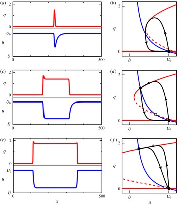
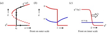
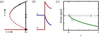
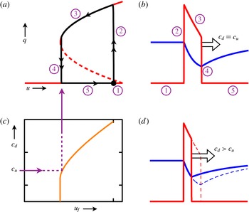
1 Introduction
More than a century ago Osborne Reynolds (Reference Reynolds1883) launched the study of turbulent transition as he sought to understand the conditions under which fluid flowing through a pipe would be laminar or turbulent. Because laminar and turbulent flow have vastly different drag laws and mixing properties, these questions are as important now as they were in Reynolds’ day. Pipe flow has now become a dominant paradigm in the study of turbulence, and is representative of a large class of wall-bounded flows, such as those in channels, ducts and boundary layers. Despite the appealing simplicity of pipe flow, the complexity of phenomena it exhibits are such that it would ultimately take more than 100 years to reach an understanding of the route to turbulence in this flow, and even now many questions remain.
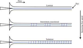
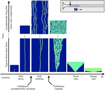
Figure 1 illustrates the most basic features established by Reynolds, and encapsulates the story I am going to tell. At low flow speeds, the fluid motion within a pipe is smooth and laminar, while at high speeds the motion quickly becomes complex and turbulent. Over some intermediate range of flow speeds, the flow is neither fully laminar nor fully turbulent, but rather a complicated combination of these two that varies over both space and time in a highly intermittent and unpredictable fashion.
The regimes of pipe flow illustrated by sketches modelled after those in Reynolds (Reference Reynolds1883). The flow here, and throughout the paper, is from left to right. At low flow speeds, the fluid motion is laminar, and dye injected at the pipe inlet produces a straight streakline. At high flow speeds, swirling motions of injected dye reveal that the fluid becomes turbulent within a short distance of the pipe inlet. The transitional regime occurs at intermediate flow speeds, where the flow exhibits irregular, intermittent turbulence.

Reynolds determined that pipe flow was governed by a single non-dimensional parameter, since referred to as the Reynolds number, which we now denote
 $$\begin{eqnarray}Re=\frac{\bar{U}d}{\unicode[STIX]{x1D708}},\end{eqnarray}$$
where
 $\bar{U}$
is the cross-sectionally averaged mean-flow speed, also known as the bulk velocity,
 $d$
is the pipe diameter, and
 $\unicode[STIX]{x1D708}$
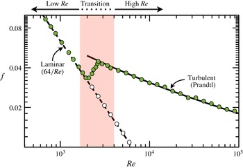
is the kinematic viscosity of the fluid. Reynolds considered many issues, but one in particular was the law of resistance for pipe flow. Essentially the question is how much pressure drop is needed to drive a given volume flux through the pipe, or vice versa. It is now standard to express this in terms of the non-dimensional friction factor as a function of
 $Re$
, as shown in figure 2. The friction factor
 $f$
is defined by
 $$\begin{eqnarray}f=\frac{\unicode[STIX]{x0394}pd}{\frac{1}{2}\unicode[STIX]{x1D70C}L\bar{U}^{2}},\end{eqnarray}$$
where
 $\unicode[STIX]{x0394}p$
is the magnitude of the pressure drop over streamwise distance
 $L$
and
 $\unicode[STIX]{x1D70C}$
is the fluid density.
Friction factor
 $f$
as a function of
 $Re$
for pipe flow. The dashed curve shows the exact relationship for fully developed laminar flow. The solid curve shows the Prandtl law for turbulent flow. Coloured points are a cartoon representation of what would be observed in a typical experiment (Schlichting Reference Schlichting1968; McKeon et al.
Reference McKeon, Swanson, Zagarola, Donnelly and Smits2004). Open points represent fully developed laminar flow that can be achieved in experiments free from disturbances that trigger turbulence. Shading indicates approximately what can be considered to be the transitional regime. It includes, but is somewhat broader than, the region where typical experiments transition from the laminar to turbulent scaling.

For my purposes this plot is useful for discussing the relationship between laminar and turbulent flows as a function of
 $Re$
. Points in the figure represent what would be measured in a typical experiment. At low
 $Re$
, the flow is laminar and the friction factor obeys the scaling easily obtained from the Navier–Stokes equations (e.g. Pope Reference Pope2000). At high
 $Re$
, the flow is turbulent and the friction factor obeys the law due to Prandtl (e.g. Schlichting Reference Schlichting1968; Pope Reference Pope2000). The much larger friction factor for turbulent flow is a quantitative expression of the increased drag due to turbulent fluid motion. Within the transition region, the flow switches from the laminar to the turbulent scaling. The shading in figure 2 is not meant to define a precise region, but rather to show the approximate range over which the dynamics is particularly interesting, and over which I will focus.
One of the most significant features of figure 2 is the open points showing what is observed in experiments free from disturbances that trigger turbulence. These indicate that turbulence is not inevitable as
 $Re$
increases through and even beyond the transition region. The transition to turbulence in pipe flow is thus subcritical, meaning that turbulence exists even without laminar flow first becoming unstable. This is common for wall-bounded shear flows (Manneville Reference Manneville2015), e.g. channel flow, duct flow, plane Couette flow and others that will not be discussed here. We know from numerical computations that laminar pipe flow is stable to infinitesimal disturbances (linear stability) to at least
 $Re=10^{7}$
(Salwen, Cotton & Grosch Reference Salwen, Cotton and Grosch1980; Meseguer & Trefethen Reference Meseguer and Trefethen2003). While no real experiment will show laminar flow at such large
 $Re$
, maintaining laminar flow at the open points shown in the figure is common in a well-controlled experiment, (e.g. Wygnanski & Champagne Reference Wygnanski and Champagne1973; Darbyshire & Mullin Reference Darbyshire and Mullin1995; van Doorne & Westerweel Reference van Doorne and Westerweel2009).
Consider now the following question: is there a critical point for the onset of turbulence in pipe flow, and if so, what is the critical Reynolds number? This fundamental question is really at the heart of Reynolds’ original study. While this specific question will not be the sole, or even the primary focus of this paper, it is useful to consider since it highlights so much about what is interesting and difficult in the transition problem. The intermittent appearance of turbulence and the subcritical character of the transition complicate this issue and require first stating precisely what the question is. I will get to that in good time. Nevertheless, as the cartoon of coloured experimental points in figure 2 indicates, a sensibly defined critical point would probably be at
 $Re\approx 2000$
, as Reynolds himself estimated in 1883. However, it was not until 2011 (Avila et al.
Reference Avila, Moxey, de Lozar, Avila, Barkley and Hof2011) that the critical value was definitely determined in a way that was fully justified and that did not suffer from finite-size effects. Determining this value required demanding experiments that could not have been performed in Reynolds’ time. As we will see, this is only one piece in the story of how turbulence arises, but it illustrates how only recently has it been possible to definitely answer some of the most basic questions about this flow and to obtain a more-or-less clear understanding of the route to turbulence in pipe flow. Manneville (Reference Manneville2015, Reference Manneville2016) gives excellent reviews of the field in the broader context of wall-bounded shear flows.
I will end this short introduction by summarizing what will be presented and how. This subject is largely driven by experiments and direct numerical simulations (DNS) of the Navier–Stokes equations. These are where the facts come from. I will refer to these facts as needed, but for the most part will use my own cartoon representations of what experiments and simulations tell us, rather than reprinting results published elsewhere. (Figures 1 and 2 already illustrate this approach. No actual measurements are shown in these figures.) I will present my perspective on the route from laminar to turbulent flow in a pipe by focusing on what can be understood from relatively few simple physical ideas and developing models that express these ideas. As already indicated, there is a rich variety of phenomena associated with pipe flow transition. Rather than first presenting all the phenomena and then discussing a theoretical framework, I will proceed little by little with increasing detail about transition process. Only at the end will I be able to fully address issues such as the critical point for pipe flow.
2 What pipe flow transition is not – a short history
In the years following Reynolds’ experiments, attempts to explain the onset of turbulence via analysis of the Navier–Stokes equations met with failure. Eckert (Reference Eckert2010) gives a review of that ‘troublesome’ period in hydrodynamic stability theory. So dire was the situation more than 20 years after Reynolds’ first work on the problem, that Orr (Reference Orr1907) wrote ‘It would seem improbable that any sharp criterion for stability of fluid motion will even be arrived at mathematically.’ This remained the case through the early 1920s when, for example, Prandtl writes to von Kármán: ‘and so, once more, we do not obtain a critical Reynolds number. There seems to be a very nasty devil in the turbulence so that all mathematical efforts are doomed to failure’ (see Eckert Reference Eckert2010, p. 43).
Taylor (Reference Taylor1923) had the great insight to considered instead a shear flow that actually possesses a linear instability. Quoting from Taylor: ‘It seems doubtful whether we can expect to understand fully the instability of fluid flow without obtaining a mathematical representation of the motion of a fluid in some particular case in which instability can actually be observed, so that a detailed comparison can be made between the results of analysis and those of experiment.’ Taylor conducted both experiments and a linear stability analysis on the flow between concentric rotating cylinders, now commonly called Taylor–Couette flow. The outstanding agreement between the two solidified linear stability analysis as a fundamental tool of fluid dynamics.
Nonlinearity presented an even greater challenge to obtaining a mathematical description of the route to turbulence. Landau (Reference Landau1944) and Stuart (Reference Stuart1958) explained how nonlinearity would come into play following a linear instability. The basic message is that nonlinearity will lead to two fundamentally different situations. In one, nonlinearity will act to arrest the growth of a linearly unstable mode (supercritical instability), while, in the other, nonlinearity will act to further enhance the growth of the unstable mode (subcritical instability). Later developments in bifurcation theory greatly extended the understanding of how nonlinearity manifests itself. This made it possible to understand not only initial (primary) instabilities, but also subsequent (secondary) instabilities in flows such as Taylor–Couette flow (see, e.g. Joseph Reference Joseph1976; Chossat & Iooss Reference Chossat and Iooss1985).
In the 1970s chaos burst onto the scene with the works of Ruelle & Takens (Reference Ruelle and Takens1971), Feigenbaum (Reference Feigenbaum1978), and others. Ruelle & Takens (Reference Ruelle and Takens1971) specifically proposed a connection between chaotic dynamics and turbulence. They suggested a modification of the earlier Landau–Hopf view that turbulence occurred after a large number of successive instabilities (Landau Reference Landau1944; Hopf Reference Hopf1948). They showed that instead only a few instabilities were necessary to generate complex, non-periodic dynamics, meaning that turbulence could appear in a fluid after only a few instabilities. This was subsequently confirmed by Gollub & Swinney (Reference Gollub and Swinney1975) in experiments on Taylor–Couette flow.
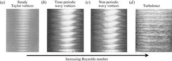
This culminated in a route to turbulence illustrated in figure 3. As the Reynolds number of the flow is increased, by increasing the rotation rate of the inner cylinder in the case shown, the system undergoes a sequence of successive instabilities. Each instability increases the complexity of the dynamics such that after a short sequence the dynamics becomes chaotic, i.e. turbulent. The volume edited by Swinney & Gollub (Reference Swinney and Gollub1985) gives a wonderful account of the success of this approach, and it communicates the excitement that followed the bringing together of dynamical system theory and hydrodynamic instabilities to understand the transition to turbulence.
Experiments illustrating the route to turbulence in Taylor–Couette flow. Photographic images show flow states encountered with increasing Reynolds number (increasing from a–d). The flow is turbulent (d) following a short sequence of successive instabilities. Modified from (Swinney & Gollub Reference Swinney and Gollub1985).

There is just one problem – this picture is essentially irrelevant to transition in pipe flow. One can end up wasting a lot of time trying to bend and contort this scenario to try to make it conform to what is observed in pipe experiments. In actuality, the route to turbulence in pipe flow is of a wholly different type, and requires a completely different perspective. If you have the above picture of transition in mind, you should forget it now. I cannot stress this enough.
(I do want to note that history also includes several individuals who understood, or would have understood, that the above picture does not apply to pipe flow. Important among them would be Rotta (Reference Rotta1956), Lindgren (Reference Lindgren1957), Landau & Lifshitz (Reference Landau and Lifshitz1959), Coles (Reference Coles1962), Wygnanski & Champagne (Reference Wygnanski and Champagne1973), and Reynolds himself. That is not meant to be a complete list, and it does not include my contemporaries. Rather than give a separate alternative history, I will refer to these important works as needed in the following.)
3 The first step – low and high Reynolds number
As a first step in understanding the transition problem, I want to take a detour and consider what happens at high and low Reynolds numbers, excluding the transition regime where the most interesting dynamics occurs. I find it useful first to develop a good understanding of dynamics outside the transitional regime and then after to build on this for a more complete explanation for transitional behaviour.
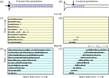
Figure 4 summarizes what I will focus on. Two common types of experiments are illustrated (e.g. Wygnanski & Champagne Reference Wygnanski and Champagne1973; Darbyshire & Mullin Reference Darbyshire and Mullin1995). In figure 4(a), the flow is constantly disturbed at or near the pipe inlet. In figure 4(b), incoming laminar flow is allowed to develop, but then is disturbed over a brief time interval, typically with a short-duration transverse jet, resulting in a localized disturbance to laminar flow. Space–time plots illustrate what measurements of transverse velocity magnitude on the pipe centreline might look like at low and high
 $Re$
for each type of disturbance.
The dynamics of pipe flow at low and high
 $Re$
. Two common types of disturbances are illustrated: (a) a constant perturbation near the pipe inlet that continually disturbs incoming flow and (b) a short-duration perturbation that only locally disturbs laminar flow. Space–time plots (c)–(f) illustrate the resulting dynamics at low and high
 $Re$
, excluding the transitional regime. The plots are not from actual pipe measurements, but resemble what might be observed for transverse velocity magnitude on the pipe axis in an experiment. The expanding turbulent state in (f) is known as a slug.

At low
 $Re$
, the flow cannot sustain turbulence. Figure 4(c,d) depicts what could be observed when
 $Re$
is not so small that turbulent fluctuations immediately dissipate. Advection by the mean-flow transports decaying turbulence some distance downstream before the system reverts to laminar flow. At high
 $Re$
, once triggered, turbulence expands at the expense of laminar flow, as illustrated in figure 4(e,f). The expanding turbulent state following the localized perturbation is known as a slug. The spreading rates on the upstream and downstream sides of the slug are key quantities of interest that have been studied extensively in experiments and numerical simulations (e.g. Coles Reference Coles1962; Lindgren Reference Lindgren1969; Wygnanski & Champagne Reference Wygnanski and Champagne1973; Nishi et al.
Reference Nishi, Ünsal, Durst and Biswas2008; Duguet, Willis & Kerswell Reference Duguet, Willis and Kerswell2010; Barkley et al.
Reference Barkley, Song, Mukund, Lemoult, Avila and Hof2015).
From the development of slugs it is known that downstream advection by the mean flow plays a significant role even at high
 $Re$
. Experiments show that advection dominates expansion such that, at least up to
 $Re\simeq 10^{5}$
, turbulence does not spread upstream from where it is triggered (Wygnanski & Champagne Reference Wygnanski and Champagne1973). The trend suggests that this will hold to much larger
 $Re$
, and possibly all values
 $Re$
.
Here we get a taste of what we must deal with in understanding actual pipe experiments. Not only must the flow be disturbed, but in addition pipes must be sufficiently long to allow the disturbed flow to obtain its asymptotic state before reaching the downstream end of the pipe. When obtaining quantities such as the friction factor (or turbulence fraction as we consider later), it is necessary that measurements be made after the flow has reached an asymptotic state. While continuous inlet disturbances provide less information on spreading rates than do localized perturbations, continuous disturbances can be better suited for producing an asymptotic state of turbulence in the downstream portion of a pipe.
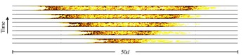
Figure 5 shows an expanding turbulent slug from a direct numerical simulation of the Navier–Stokes equations. Periodic boundary conditions are employed at the ends of a pipe
 $50d$
in length. For ease of visualization, snapshots of the flow have been translated and displayed in a frame of reference moving at the mean velocity
 $\bar{U}$
. In the laboratory reference frame in which the pipe is stationary, the slug centre advects approximately
 $40d$
downstream over the time shown. This means that, in the laboratory reference frame, the upstream (left) edge of the slug advects downstream faster than it expands, as illustrated in figure 4(f).
Expansion of a turbulent slug as seen in a frame of reference moving at the mean-flow velocity
 $\bar{U}$
. Results are from a DNS of pipe flow at
 $Re=4000$
. The kinetic energy of the flow, with laminar Hagen–Poiseuille flow subtracted, is visualized in a cross-section through the pipe. Thus, laminar Hagen–Poiseuille flow appears as white. The five snapshots are separated by 10 advective time units
 $d/\bar{U}$
. The pipe has length
 $50d$
, with periodic boundary conditions imposed in the streamwise direction. In the reference frame in which the pipe is stationary, turbulence does not expand upstream from where it is triggered. (Simulation courtesy of M. Chantry.)

Numerical simulations with periodic boundary conditions can alleviate some of the requirements for very long pipes needed in experiments, by effectively decoupling long temporal evolution from long spatial evolution. Much depends on what the question is, but it is not uncommon to be interested in the long-time behaviour of structures no greater than
 $100$
pipe diameters. The simulation shown is a relatively small in both space and time. It is constrained by the need to visualize the resulting flow state rather than by the computational resources needed to produce it.
Before leaving these issues, I will take the opportunity to comment on the connection between what is illustrated in figure 4 and the concepts of absolute and convective instability (Chomaz Reference Chomaz2005). At a linear level, laminar pipe flow is always stable. As a result, linear instability, whether absolute or convective, will not appear anywhere in the following; everything of interest will be nonlinear. At a nonlinear level, the expansion of turbulent slugs is dominated by downstream advection such that, at least to
 $Re\simeq 10^{5}$
, turbulence resulting from a localized perturbation always advects out of the system in the laboratory reference frame. Such flows can be classified as nonlinearly convectively unstable (Chomaz Reference Chomaz2005).
4 The almost correct analogy – phase transitions
It has been long been recognized that the distinct regions of turbulent and laminar fluid motion observed in many shear flows have analogies to coexisting phases in thermodynamic systems, and moreover that the interfaces between the turbulent and laminar regions are key to understanding these flows. Coles (Reference Coles1962) summarizes the situation so well that I find it is best to quote him directly: ‘Among several related questions raised by this study of interfaces and intermittency, one of the most important concerns the remarkable stability of the mixed flows already described. It seems that nature does not ordinarily provide a continuous range of states varying from fully laminar to fully turbulent flow. If both types of flow are present they are distinct, in the same sense that the liquid and gaseous states are distinct for any ordinary fluid. At least in the case of transition, the turbulent regions have a characteristic geometry and characteristic propagation velocity which are so regular that a definite mechanism must be involved.’
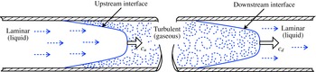
Figure 6 illustrates the points Coles is making. This figure is itself modelled after the depiction of a turbulent slug in Wygnanski & Champagne (Reference Wygnanski and Champagne1973). The flow is composed of two types of motion – laminar and turbulent – and these regions are separated by sharp interfaces rather than a gradual variation between the two flow types. The figure is schematic, and on some level there is continuous variation, but to a good approximation this is the situation for intermittent flows. One can think of the turbulent region as the more disordered gaseous phase and the laminar region as the liquid phase. The speeds of these interfaces are particularly important.
Illustration, modelled after Wygnanski & Champagne (Reference Wygnanski and Champagne1973), showing the structure of a turbulent slug. A region of turbulent flow is bounded upstream and downstream by laminar flow. The middle portion of the slug is not shown. Laminar flow can be viewed as a liquid phase, while the disordered turbulent fluid motion can be viewed as a gaseous phase. Sharp interfaces, or fronts, separate the laminar and turbulent regions. The speed of the upstream interface,
 $c_{u}$
, and the speed of the downstream interface,
 $c_{d}$
, play key roles in the dynamics of the system.

While Wygnanski & Champagne (Reference Wygnanski and Champagne1973) provide details on the turbulent energy budget in the vicinity of both upstream and downstream interfaces (extending previous considerations by Rotta (Reference Rotta1956) and Coles (Reference Coles1962)), these results do not, or I should perhaps say have not, led to expressions for interface speeds. Lindgren (Reference Lindgren1969) attempts an expression for the speed of the upstream interface. While the approach is interesting, the result unfortunately is unsatisfactory.
Pomeau (Reference Pomeau1986) had the significant insight to consider generic features of interfaces between two coexisting states or phases. The idea is that front speed provides a notion of stability and metastability for systems with multiple stable states, and that simple considerations, independent of the precise details of turbulent flows, are sufficient to understand much of the large-scale dynamics of subcritical shear flows. (Earlier, Landau & Lifshitz (Reference Landau and Lifshitz1959) had noted that the notion of metastability applied in the context of subcritical shear flows, and pipe flow in particular, but did not develop the idea further. See Pomeau (Reference Pomeau2015) for a recent review of the subject.) This is a very important part of the story that I will now explain in detail.
4.1 Local dynamics
First I need to address the turbulent dynamics in the absence of interfaces. Figure 7 illustrates the idea. Shown is a DNS of turbulent flow at
 $Re=4000$
in a short pipe with streamwise periodic boundary conditions. The
 $2.5d$
axial length is near the minimal size that can sustain turbulent structures at this
 $Re$
. Effectively, this is a simulation of the turbulence in the core of the expanding slug in figure 5. I will refer to the dynamics of such a small domain as the local dynamics or spatially homogeneous dynamics. The spatial variations seen in figure 7(a) are on a microscopic scale from the present point of view. (See Waleffe (Reference Waleffe1997), Faisst & Eckhardt (Reference Faisst and Eckhardt2003), Wedin & Kerswell (Reference Wedin and Kerswell2004), Eckhardt et al. (Reference Eckhardt, Schneider, Hof and Westerweel2007), Kawahara, Uhlmann & van Veen (Reference Kawahara, Uhlmann and van Veen2012) for details of the coherent structures of wall-bounded turbulence, structures that will be here treated as microscopic. Pomeau (Reference Pomeau2015) discusses at length the issues of considering turbulence as a microscopic state in analogy with atoms in standard statistical mechanics.)
There are three perspectives on the temporal dynamics within this small box. The first, figure 7(b), is a detailed view in which the turbulent dynamics is chaotic. The second, figure 7(c), is the coarsest view in which turbulence is simply a equilibrium point. This is a reasonable perspective looking at, for example, the integrated turbulent kinetic energy, where the balance of turbulent production
 $\mathscr{P}$
and dissipation
 $\unicode[STIX]{x1D716}$
results in a stable equilibrium. In the third perspective, figure 7(d), the turbulent dynamics is viewed as a stable state subjected to random fluctuations. Regardless of how one chooses to view the turbulence, at this value of
 $Re$
the local dynamics exhibits bistability between turbulence and laminar flow.
Local dynamics of pipe flow in the absence of interfaces. (a) Snapshot of turbulent flow from a DNS at
 $Re=4000$
in a short pipe with periodic boundary conditions. This turbulent state is viewed as the local state, corresponding to the turbulent core of the slug in figure 5. The spatial variation within this domain is viewed as microscopic. The dynamics of this local turbulent state can be viewed as: (b) chaotic, (c) an equilibrium where production
 $\mathscr{P}$
balances dissipation
 $\unicode[STIX]{x1D716}$
, or (d) an equilibrium subjected to random fluctuations. Coexisting with turbulent flow is laminar Hagen–Poiseuille flow.

Much can be learnt in the simplest case where turbulence is viewed as a fixed point, and so this is where we will begin. Let the local state of the system be represented by a single scalar variable
 $q\geqslant 0$
that represents an ‘amplitude of turbulence’, with
 $q=0$
corresponding to laminar flow and
 $q>0$
corresponding to turbulent flow. I will typically refer to
 $q$
as the turbulence level or the turbulence intensity. We then take the local dynamics to be of the form
 $$\begin{eqnarray}\dot{q}=f(q)=-\frac{\text{d}V\,(q)}{\text{d}q}.\end{eqnarray}$$
In terms of the analogy with phase transitions, the potential
 $V(q)$
is like the free-energy density of the bulk phases. Above a certain Reynolds number, the potential will be a double-well with minima corresponding to laminar and turbulent flow. I do not mean to imply that the local dynamics can actually be reduced to variational form, but the potential provides useful physical insights. (See appendix A.) Later I will consider a non-variational model that more completely captures the local dynamics of the Navier–Stokes equations.
For concrete illustration, I will use the following potential,
 $$\begin{eqnarray}V(q)=\frac{q^{2}}{2}\left[\unicode[STIX]{x1D6FF}+(r+\unicode[STIX]{x1D6FF})\left(\frac{q^{2}}{2}-\frac{4q}{3}\right)\right],\end{eqnarray}$$
where
 $r$
is a parameter playing the role of Reynolds number and
 $\unicode[STIX]{x1D6FF}$
is a fixed constant. (Throughout this section
 $\unicode[STIX]{x1D6FF}$
will be fixed at
 $\unicode[STIX]{x1D6FF}=8$
. Later
 $\unicode[STIX]{x1D6FF}$
will be set to a smaller value.) The local dynamics of
 $q$
is thus given by
 $$\begin{eqnarray}\dot{q}=-\frac{\text{d}V\,(q)}{\text{d}q}=f(q)=q\left[r-(r+\unicode[STIX]{x1D6FF})(q-1)^{2}\right].\end{eqnarray}$$
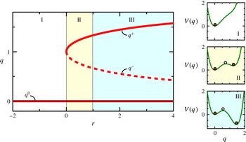
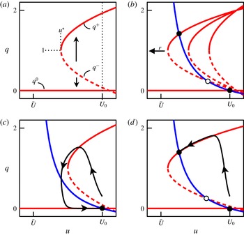
Figure 8 shows a bifurcation diagram for the local dynamics, together with the potential at three representative values of
 $r$
. Steady states are extrema of
 $V$
or roots of
 $f$
. For
 $r<0$
the only steady state is
 $q^{0}=0$
. At
 $r=0$
the potential develops an inflection point, corresponding to a saddle-node bifurcation, and for
 $r>0$
there are three branches of solutions
 $$\begin{eqnarray}q=\left\{\begin{array}{@{}ll@{}}q^{+}=1+\sqrt{{\displaystyle \frac{r}{r+\unicode[STIX]{x1D6FF}}}}\quad \quad & \text{(upper branch)},\\ q^{-}=1-\sqrt{{\displaystyle \frac{r}{r+\unicode[STIX]{x1D6FF}}}}\quad \quad & \text{(lower branch)},\\ q^{0}=0\quad & \text{(laminar)}.\end{array}\right.\end{eqnarray}$$
The upper branch
 $q^{+}$
is linearly stable (a local minimum of the potential) while the lower branch
 $q^{-}$
is unstable.
The potential thus captures the most elementary features of a subcritical shear flow. For small Reynolds number, here
 $r<0$
, laminar flow is the only equilibrium, and all initial conditions relax to this state. For sufficiently large Reynolds number, here starting at
 $r=0$
, turbulent states appear. The upper and lower branches can be thought of as a simple representation of the upper and lower branches of exact coherent structures in pipe flow (e.g. Faisst & Eckhardt Reference Faisst and Eckhardt2003; Wedin & Kerswell Reference Wedin and Kerswell2004; Eckhardt et al.
Reference Eckhardt, Schneider, Hof and Westerweel2007; Duguet, Willis & Kerswell Reference Duguet, Willis and Kerswell2008). The unstable lower branch sets the basin boundary between laminar and turbulent flow. While the laminar branch is linearly stable for all
 $r$
, its basin of attraction shrinks with increasing
 $r$
, via a power law
 $q^{-}\sim r^{-1}$
. This is consistent with the behaviour of pipe flow (Hof, Juel & Mullin Reference Hof, Juel and Mullin2003).
Local model dynamics. Shown is the bifurcation diagram of equilibrium states, with solid and dashed curves indicating linearly stable and unstable states, respectively. Also shown is the potential
 $V(q)$
at representative values of
 $r$
. Filled points are linearly stable states and open points are linearly unstable states. The laminar branch
 $q^{0}$
exists for all
 $r$
. Upper
 $q^{+}$
and lower
 $q^{-}$
branches exist for
 $r>0$
. The upper and laminar branch are always linearly stable (local minimum of
 $V$
). In region II, the laminar equilibrium
 $q^{0}$
is at a lower potential than
 $q^{+}$
, while in region III the situation is reversed.

4.2 Fronts
Now consider a long pipe in which the turbulence intensity can vary in space. The cross-sectional structure of the flow has already been discarded in describing the flow with a scalar variable
 $q$
. Hence, from the large-scale, or macroscopic point of view, the pipe has just one spatial dimension, the axial direction
 $x$
.
Pomeau (Reference Pomeau1986, Reference Pomeau2015) argues for taking the evolution equation for
 $q(x,t)$
to be of the form
 $$\begin{eqnarray}\frac{\unicode[STIX]{x2202}q}{\unicode[STIX]{x2202}t}+U\frac{\unicode[STIX]{x2202}q}{\unicode[STIX]{x2202}x}=f(q)+D\frac{\unicode[STIX]{x2202}^{2}q}{\unicode[STIX]{x2202}x^{2}},\end{eqnarray}$$
where
 $U$
is a constant representing mean downstream advection and
 $D$
is the diffusion coefficient. This is essentially the simplest, low-order extension of the local dynamics that contains both advection and diffusive coupling in space. While Pomeau (Reference Pomeau1986) did not originally include an advection term
 $U\,\unicode[STIX]{x2202}q/\unicode[STIX]{x2202}x$
, it will be very important later, so it is useful to include here.
We want to know what will be observed in the spatially extended system at parameter values such that both the upper branch and laminar branches are linearly stable (
 $r>0$
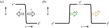
in the model). Pomeau argued that, in analogy with phase transitions, the notion of metastability applies to coexistence of laminar and turbulent flow, and that this can be deduced by examining the motion of fronts connecting the local equilibria. Specifically, consider initializing the model system with a front, or interface, smoothly connecting the two locally stable equilibria
 $q^{+}$
and
 $q^{0}$
, as shown in figure 9(a). The basic question then is: in which direction does this front move? In this spatially extended context this is what dictates the difference between stable and metastable states: the stable state invades the metastable state.
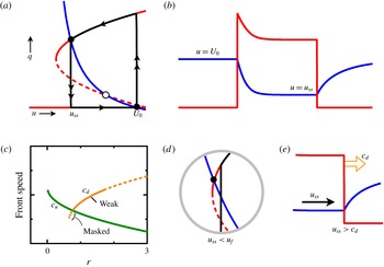
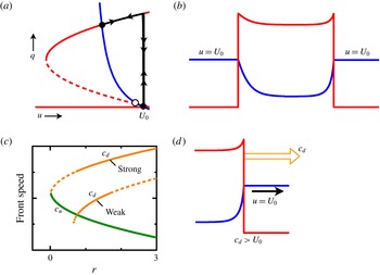
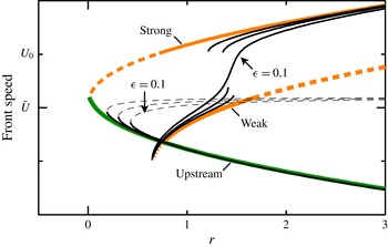
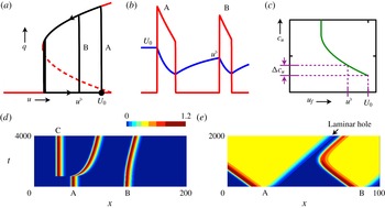
For the simple model, the local dynamics is described by a potential, and one can simply read off, as in figure 8, the relative stability of the two equilibria. In region II, the laminar fixed point is at a lower potential than the upper-branch fixed point. Hence, while both are locally stable points, the laminar fixed point is ‘preferred’ over the turbulent one. That is, laminar flow is stable while turbulent flow is metastable. In region III, the situation is reversed, and laminar flow is metastable with respect to turbulent flow. The relative stability of the two locally stable fixed points is a property of the local dynamics (the potential
 $V$
) and is independent of the advection speed
 $U$
.
Fronts between turbulent
 $q^{+}$
and laminar
 $q^{0}$
states. (a) Illustration of the basic question: which direction does a front move? This dictates which state is stable and which state is metastable. (b) Upstream and downstream fronts surrounding a region of turbulence (slug). The fronts move with speeds
 $c_{u}$
and
 $c_{d}$
as shown. The fronts are taken to be well separated such that they behave as isolated fronts.

I will now analyse the front motion without assuming the existence of a potential. While the analysis is very simple, it is useful to include the details for future reference. Moreover, when advection is present, one must be clear about the meaning of invasion, and this analysis will highlight this aspect.
Consider the front solution after any initial transients have died down so that the front is travelling at constant speed, denoted
 $c$
, which may be positive (motion to the right) or negative (motion to the left). Make a coordinate transformation to go into a co-moving frame of reference at speed
 $c$
,
 $$\begin{eqnarray}z=x-ct,\end{eqnarray}$$
and locate the now stationary front at
 $z=0$
. The steady front satisfies
 $$\begin{eqnarray}(U-c)\frac{\text{d}q}{\text{d}z}=f(q)+D\frac{\text{d}^{2}q}{\text{d}z^{2}}.\end{eqnarray}$$
Now make a further coordinate change to natural inner coordinate for the front,
 $$\begin{eqnarray}\unicode[STIX]{x1D709}=\frac{z}{\sqrt{D}},\end{eqnarray}$$
and define
 $$\begin{eqnarray}s\equiv \frac{c-U}{\sqrt{D}}.\end{eqnarray}$$
Then the equation for the steady front becomes
 $$\begin{eqnarray}q^{\prime \prime }+sq^{\prime }+f(q)=0,\end{eqnarray}$$
together with boundary condition at infinity
 $$\begin{eqnarray}q(-\infty )=q^{+},\quad q(+\infty )=q^{0}.\end{eqnarray}$$
Primes denote
 $\text{d}/\text{d}\unicode[STIX]{x1D709}$
and
 $s$
is referred to as a nonlinear eigenvalue.
Generically, there will be a solution to (4.10) and (4.11) for a unique value of
 $s$
. (See appendix A.) This solution determines both the shape of the front
 $q(x)$
and its speed via
 $s$
. As both
 $f(q)$
and
 $q^{+}$
depend on the parameter
 $r$
, the nonlinear eigenvalue
 $s$
will depend on
 $r$
as well, so denote this
 $s(r)$
.
In addition to fronts going from
 $q^{+}$
to
 $q^{0}$
with increasing
 $x$
, there are also those going from
 $q^{0}$
to
 $q^{+}$
, as illustrated in figure 9(b). We always assume fronts are well separated and such that they can be analysed independently. The front on the left would be an upstream front and the one on the right would be the downstream front. In the analysis, the only difference between the upstream front and the downstream front is the boundary conditions applied. For the upstream front the boundary conditions are the reverse of (4.11), namely
 $$\begin{eqnarray}q(-\infty )=q^{0},\quad q(+\infty )=q^{+}.\end{eqnarray}$$
However, reversing the boundary conditions is equivalent to reflecting in
 $\unicode[STIX]{x1D709}$
,
 $\unicode[STIX]{x1D709}\rightarrow -\unicode[STIX]{x1D709}$
. This reflection changes only the sign of the odd derivative in (4.10). Hence, the upstream front is obtained merely by reflecting the downstream front and changing
 $s$
to
 $-s$
. Thus, it is sufficient to solve (4.10) subject to (4.11) for various values of
 $r$
, then from
 $s(r)$
the speeds of the upstream and downstream fronts are given by
 $$\begin{eqnarray}\displaystyle & c_{u}=U-\sqrt{D}\,s(r), & \displaystyle\end{eqnarray}$$
 $$\begin{eqnarray}\displaystyle & c_{d}=U+\sqrt{D}\,s(r). & \displaystyle\end{eqnarray}$$
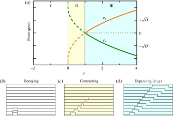
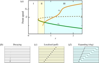
Figure 10 shows the speeds of upstream and downstream fronts from numerical solutions to (4.10) and (4.11). The speeds are symmetric about the advection speed
 $U$
. Here
 $D=1$
, but the value does not affect the transition points or the qualitative behaviour. In region II,
 $c_{d}<c_{u}$
and the fronts move towards one another, that is, the laminar state
 $q^{0}$
invades the turbulent state
 $q^{+}$
; hence, laminar flow is stable while turbulence is metastable. At
 $r=1$
the front speeds cross. In region III,
 $c_{d}>c_{u}$
and turbulence invades laminar flow, indicating that now laminar flow is metastable with respect to turbulence.
Behaviour of model fronts. The upper plot (a) shows speeds of upstream and downstream fronts as a function of model Reynolds number
 $r$
. Below are space–time plots of turbulence intensity
 $q$
at representative values of
 $r$
: (b)
 $r=-1$
, (c)
 $r=0.5$
and (d)
 $r=2$
. For
 $r<0$
, region I, the upper turbulent equilibrium does not exist, so fronts between
 $q+$
and
 $q^{0}$
are meaningless. The initial condition for space–time plot (b) has a region
 $q>0$
, which rapidly decays in time. (The time scale of this plot is 20 times shorter that of the other two space–time plots.) For
 $0<r<1$
, region II, the upper turbulent state exists, but is metastable with respect to laminar flow. The turbulent patch contracts. For
 $1<r$
, region III, laminar flow is metastable with respect to turbulence. Turbulence expands by invading laminar flow.

Qualitatively, the behaviour in figure 10 had been anticipated from the relative depths of the potential
 $V$
at the laminar and turbulent fixed points, as shown in figure 8. The analysis of front speeds provides more quantitative information, and it does so by a method that does not rely on the existence of a potential. The key point is the relationship between front speeds (4.13) and the nonlinear eigenvalue
 $s$
obtained from (4.10) and (4.11). Front speeds are determined by two terms. One is merely kinematic advection at speed
 $U$
. This is independent of the type of front. The other term is dynamical, and corresponds to the front motion relative to the kinematic advection. This changes sign with front type, and dictates whether turbulent flow invades laminar flow or vice versa. It provides the answer to the question posed in figure 9. Since
 $c_{d}-c_{u}=2\sqrt{D}\,s(r)$
, if
 $s(r)<0$
then fronts evolve so as to decrease the fraction of flow in the turbulent state, while if
 $s(r)>0$
then fronts evolve so as to increase the fraction of turbulence flow. Later we will see a similar structure arise from the analysis of a more elaborate model in which the underlying advection is not constant.
4.3 Further details
There are a few other relevant features of the model that I want to cover briefly. In order not to lose focus, I will leave the details to appendix A. Some of the techniques presented there will be useful later, but they are not essential at the moment.
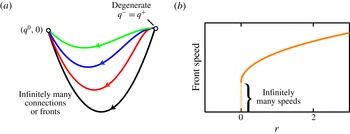
First, I want to note what happens at the limit point where the upper- and lower-turbulent branches coalesce and where the fronts terminate:
 $r=0$
in figures 8 and 10. At this point the upper-branch fixed point ceases to be hyperbolic, and this in turn means that fronts cease to be uniquely selected. The speed can take on any of a range of values. (See appendix A.) Just above this point,
 $r>0$
, the front speeds exhibit a square-root scaling with
 $r$
. However, given this occurs in the region where turbulence is strongly contracting, the scaling is effectively masked.
The second point of interest is the transition point between contracting and expanding turbulence:
 $r=1$
in the model. Because the front speeds cross transversely, the scaling of the expansion rate with Reynolds number has a trivial exponent:
 $c_{d}-c_{u}\sim (r-1)^{\unicode[STIX]{x1D6FE}}$
, where
 $\unicode[STIX]{x1D6FE}=1$
. Exactly at
 $r=1$
, the solution to (4.10) gives
 $s=0$
, for both upstream and downstream fronts. Essentially, there is no driving mechanism for fronts to move in either direction, other than advection by the mean speed
 $U$
. Such fronts are said to be neutral. When the local dynamics is derivable from a potential, it can be shown (see appendix A) that the neutral fronts must correspond to
 $$\begin{eqnarray}V(q^{0})=V(q^{+}).\end{eqnarray}$$
This is the intuitively obvious condition that the transition between contracting and expanding turbulence occurs precisely where the potentials of the laminar and turbulent state are equal.
Finally, in addition to fronts connecting laminar flow and the stable turbulent state, the model has small-amplitude unstable travelling waves. In the context of shear flows these are known as edge states (Schneider, Eckhardt & Yorke Reference Schneider, Eckhardt and Yorke2007; Eckhardt et al. Reference Eckhardt, Schneider, Hof and Westerweel2007), because they are on the edge between laminar and turbulent flow. Their stable manifolds determine the basin boundary separating initial conditions that decay to laminar flow and those that grow to turbulent flow.
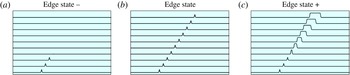
Figure 11 illustrates the behaviour of edge states in the model. Panel (b) shows the edge state itself. It is a localized, unstable travelling state. Panels (a) and (c) show the evolution from small perturbations of the edge state (either slightly decreasing or increasing the size of
 $q$
). From the point of view of spatial dynamics (see appendix A) edge states are homoclinic connections from the laminar branch
 $q^{0}$
to itself. For the model, one can easily show that the edge states satisfy
 $s=0$
, and hence have speed
 $c=U$
. These exist for all
 $r>1$
. As
 $r$
decreases towards 1, their amplitude increases, and at
 $r=1$
they coalesce with the neutral fronts.
Space–time plots of the model edge state at
 $r=2.0$
. (b) The edge state is a low-amplitude, localized travelling pulse. (a,c) show evolution from the slightly perturbed edge state. A slight decrease in
 $q$
results in decay to laminar flow (a), while a slight increase in
 $q$
results in an expanding slug (c).

4.4 Fluctuations
I presented three views of the local dynamics in figure 7. While we learnt much by treating turbulence as a fixed equilibrium, a more realistic description of pipe flow would incorporate fluctuations in the turbulent phase. Arguably the simplest approach to introducing fluctuations, while maintaining a description with a single real amplitude, is to introduce multiplicative noise into the local dynamics (Barkley Reference Barkley2011b ; Pomeau Reference Pomeau2015). That is, the local dynamics given by (4.1) is modified to be
 $$\begin{eqnarray}\dot{q}=f(q)+\unicode[STIX]{x1D70E}q\unicode[STIX]{x1D702},\end{eqnarray}$$
where
 $\unicode[STIX]{x1D70E}$
is a parameter controlling the noise strength. I will take
 $\unicode[STIX]{x1D702}$
to be white Gaussian noise with unit variance, although other forms could be considered. The noise term in (4.15) models only the intrinsic turbulent fluctuations (which in reality are deterministic), and not randomness due to external influences. The multiplicative form of the noise ensures that laminar flow,
 $q=0$
, is free from fluctuations. Including space, the evolution equation for
 $q$
becomes
 $$\begin{eqnarray}\frac{\unicode[STIX]{x2202}q}{\unicode[STIX]{x2202}t}+U\frac{\unicode[STIX]{x2202}q}{\unicode[STIX]{x2202}x}=f(q)+D\frac{\unicode[STIX]{x2202}^{2}q}{\unicode[STIX]{x2202}x^{2}}+\unicode[STIX]{x1D70E}q\unicode[STIX]{x1D702}.\end{eqnarray}$$
In this case
 $\unicode[STIX]{x1D702}$
is white in both space and time.
I will discuss the noise case further later in the paper. Here I only want to show what the model produces when fluctuations are included. In fact, I have already shown these. The space–time plots in figure 4 are numerical solutions to (4.16) at
 $r=0.2$
(the low-Reynolds-number example) and
 $r=3$
(the high-Reynolds-number example). Parameter values are:
 $\unicode[STIX]{x1D6FF}=8$
,
 $D=1$
,
 $U=4$
and
 $\unicode[STIX]{x1D70E}=0.2$
. (Further information about models and simulations can be found in appendix B.) For the simulations corresponding to constant incoming disturbance,
 $q$
is set to
 $q^{+}$
over an interval at the left side of the domain. Plotted are just the fluctuations,
 $|\unicode[STIX]{x1D70E}q\unicode[STIX]{x1D702}|$
, as these mimic what might be observed for the magnitude of the transverse velocity fluctuations on the centreline. These solutions capture the broad features of pipe flow in the low- and high-Reynolds-number regimes.
4.5 Discussion
What I have done in this section is write down, analyse, and simulate explicit model equations for ideas expressed previously by others, notably Landau, Coles, and especially Pomeau. I have done this for two reasons. The first is that I find it preferable to illustrate concepts with specific solutions, such as in figure 4. The second reason is that shortly I will build on this model to explain a more complete theory of transition.
The simple model provides a base scenario for the route to turbulence in pipe flow. It clearly distinguishes the notion of local stability from stability in a spatially extended context, and it highlights the role of downstream advection. The ingredients are few: three branches of local equilibria, advection and diffusive coupling. The turbulent upper branch is locally a stable steady state, and yet when it first appears it is metastable with a very specific meaning – namely that a front between turbulent and laminar flow will move in the direction that decreases the turbulence fraction. Laminar flow is favoured. At some larger Reynolds number, the situation reverses. Now turbulence is favoured and fronts connecting turbulent and laminar flow will move in the direction that increases the turbulent fraction of flow. This corresponds to the gross feature of slugs in pipe flow. Simultaneous with the formation of expanding slugs, localized edge states appear whose stable manifolds determine the threshold perturbations giving rise to transition.
I will end this section by re-emphasizing a point crucial to the correct understanding of pipe flow. As discussed at the end of § 4.2, one must clearly separate the truly dynamical aspects of front motion from the kinematic effects due to advection. Consider the upstream (left) fronts of the expanding slugs in figures 4(f) and 10(d). Looking at these fronts in isolation, one might be tempted to think that they correspond to what is called a reverse transition, where fluid in the turbulent state transitions or relaxes to laminar flow (Narasimha & Sreenivasan Reference Narasimha and Sreenivasan1979). After all, at a fixed spatial location one can observe the system in the turbulent state at one time instant and in the laminar state at a later time. However, what is actually happening is that turbulent flow is invading laminar flow at the upstream front, but dominant advection is driving everything downstream. We will return to this soon, and repeatedly.
5 So what is the problem?
The preceding theory provides a simple and appealing description of the dynamics of turbulent structures at low and high Reynolds numbers. In fact, if the dynamics at low and high
 $Re$
were the whole story, I could simply declare victory now. The scalar model contains the basic mechanisms for front motion, and for my purposes it is quite good at capturing the essential large-scale (macroscopic) dynamics of pipe turbulence outside of the transitional region.
So what is the problem? The problem is that while the simple theory gets many things correct, it fails fundamentally when it comes to describing the dynamics within the transition regime. The reason – at the very point where turbulence first begins to appear, it occurs in the form of persistent localized patches.
I now need to begin describing the nature of transitional turbulence, the turbulence already illustrated in figure 1. The full story is rather complex, and for the moment I will focus just on the basics of localized turbulence. Later in the paper I will turn to the dynamics of localized structures on long time scales, and how this plays a crucial role in the transition process.
DNS of a turbulent puff in pipe flow at
 $Re=2000$
. The kinetic energy of the flow (with laminar flow subtracted) is plotted in a cross-section through the pipe. The vertical scale is stretched by a factor of 2. The four snapshots are separated by 200 advective time units
 $d/\bar{U}$
, and are shown in a frame of reference moving at the mean-flow speed
 $\bar{U}$
. While the flow dynamics within the puff is complicated, the size and shape of the structure, level of fluctuations, and the propagation speed all remain essentially constant throughout the temporal evolution. (Simulation courtesy of M. Chantry.)

Figure 12 shows a typical localized turbulent patch from a direct numerical simulation of pipe flow at a typical transitional Reynolds number,
 $Re=2000$
. Such a localized turbulent patch is called a puff (e.g. Wygnanski, Sokolov & Friedman Reference Wygnanski, Sokolov and Friedman1975; Darbyshire & Mullin Reference Darbyshire and Mullin1995). From the four snapshots it can be seen that while the flow is turbulent, the turbulence neither expands nor shrinks, but maintains an approximately constant streamwise extent. This is in stark contrast to the expanding turbulent slugs discussed previously. The turbulent puff moves downstream at nearly fixed speed, and is here shown in a co-moving frame of reference. At it happens, for the case shown,
 $Re=2000$
, the speed is almost identical to the mean-flow speed
 $\bar{U}$
, and hence this puff remains at nearly a fixed position in the reference frame moving at this speed. While only four frames over modest time intervals are shown in figure 12, at this value of
 $Re$
the turbulence will persist almost indefinitely in this localized, solitary form (Wygnanski et al.
Reference Wygnanski, Sokolov and Friedman1975; Darbyshire & Mullin Reference Darbyshire and Mullin1995; Nishi et al.
Reference Nishi, Ünsal, Durst and Biswas2008).
Puffs, once they form, are independent of how the turbulence is triggered. The flow in figure 12 was initially seeded with a localized disturbance. However, if one had disturbed the flow by a continuous inlet perturbation, or if one had started with fully turbulent flow at higher
 $Re$
and reduced the value of
 $Re$
, or if one had made some other disturbance to laminar flow, after some initial transience the resulting turbulence at this
 $Re$
would still necessarily be localized. The flow simply will not contain any turbulent patches larger (or smaller) than the characteristic puff size (e.g. van Doorne & Westerweel Reference van Doorne and Westerweel2009; Moxey & Barkley Reference Moxey and Barkley2010; Samanta, De Lozar & Hof Reference Samanta, De Lozar and Hof2011). Depending on the length of the pipe, the flow would probably not contain a single puff, as in figure 12, but multiple puffs, as in figure 13. As illustrated, puffs are not normally observed to occur at regular intervals, but instead in an irregular, intermittent form. Sometimes the separation between puffs can be quite large. Puffs are, however, separated by a minimum distance (Samanta et al.
Reference Samanta, De Lozar and Hof2011), which is a reflection of the localized form of turbulence.
Puffs are not only persistent in time, but they are also persistent over a range of Reynolds number. That is, one does not have to tune
 $Re$
to one specific value in order to obtain localized turbulence. This is a key point. In pipe flow, throughout the range of Reynolds numbers where turbulence first can be triggered, if the flow is turbulent then that turbulence necessarily takes the form of localized puffs. At a given Reynolds number, turbulent puffs all have the same characteristic mean size and structure, and they all move with the same mean characteristic streamwise velocity.
Sketch, modelled after that appearing in Reynolds (Reference Reynolds1883), illustrating the nature of intermittent turbulent puffs in the transitional regime. Puffs of a characteristic size are observed to occur intermittently in an otherwise laminar background flow.

The previous theory (§ 4) misses the flow physics responsible for generating localized puffs, and hence it is doomed to fail in too many important respects when it comes to describing quantitatively the route to turbulence in pipe flow. Think about our phase-transition analogy. In this analogy, a localized turbulent patch would correspond to a persistent localized region in the gas phase that simultaneously experiences a liquid-to-vapour transition on one side, and a vapour-to-liquid on the other, exactly as needed to maintain a constant-sized gas bubble. This is clearly un-physical and the analogy is flawed.
6 A better analogy
We must abandon the analogy with phase transitions if we are to develop a correct theory for the route to turbulence in pipe flow. A near-perfect analogue is what are called excitable and bistable media (Barkley Reference Barkley2011a , Reference Barkley2012; Barkley et al. Reference Barkley, Song, Mukund, Lemoult, Avila and Hof2015). In particular, there is a strong connection between the dynamics of transitional pipe flow and the dynamics of the most common example of an excitable medium – the neuron.
6.1 Puffs and action potentials
As motivation, I first want to compare the behaviour of pipe flow at a typical transition Reynolds number,
 $Re=2000$
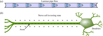
say, to the behaviour of a typical nerve cell. Figure 14(a) illustrates pipe flow in the laminar state. In the absence of external perturbations, the flow will remain laminar indefinitely for as long as one maintains flow through the pipe – laminar flow is linearly stable. Figure 14(b) illustrates a nerve cell. The extended portion, the axon, is used to send signals to other, distant cells. In the resting state, there is a surplus of negatively charged ions in the interior relative to the exterior of the cell. This is manifested as a voltage difference across the cell membrane separating the inside and outside of the cell. This voltage difference is easy to measure experimentally, and is called the membrane potential. Just as with the laminar state for pipe flow, the resting state is linearly stable and, in the absence of perturbation, the cell will remain indefinitely in this state as long as the cell is kept alive. The nerve cell is said to be excitable because, while it is linearly stable, it can be excited by external inputs.
Analogy between pipe flow and neurons: the resting state. (a) Pipe flow and (b) a nerve cell are illustrated in their linearly stable resting state, also referred to as the quiescent state. In principle, both systems can maintain these states indefinitely.

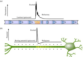
Analogy between pipe flow and neurons: the excited state. (a) A puff in pipe flow. The line plot shows the kinetic energy (laminar flow subtracted) on the pipe axis from a direct numerical simulation of a puff. (b) Action potential for a nerve axon. The line plot shows the membrane potential from simulations of the Hodgkin–Huxley model.

Now consider what happens following a short-duration, localized perturbation. For the pipe this might be the small injection of fluid through a hole in the pipe wall, as in figure 4(b). For the nerve cell, this would typically be the injection of a small current through the cell membrane. Figure 15(a) illustrates the resulting puff in pipe flow. While the pipe and shear profile are artist’s representations, the plot is simulation data from pipe flow. Figure 15(b) illustrates the analogous situation for the nerve cell (Hodgkin & Huxley Reference Hodgkin and Huxley1952). There is a localized excitation in which the sign of the membrane potential is reversed. This localized excitation in the membrane potential (known as an action potential) propagates along the nerve axon, and this is the mechanism by which nerve cells transmit signals. Once an action potential is generated, its magnitude, size and propagation speed are determined by cell properties, and is independent of how it was initially generated (just as for a puff).
I find it remarkable that this close analogy between pipe flow, and subcritical shear flows generally, and excitable systems, such as nerve cells, was not noted long ago. Perhaps it has been, but I have found no reference to it. In both cases one uses nearly identical words in describing what happens – the system is linearly stable, but there is a threshold or basin boundary such that if the system is perturbed beyond that threshold, a persistent, large-amplitude localized response is generated. The physics is very different in the two systems, but the processes of localization are essentially identical. Localized excitation persists only by continuously exciting quiescent media. A negative feedback mechanism follows excitation such that no individual part of the system stays in the excited state. This negative feedback keeps excitations from expanding and maintains separation between excitations. As already suggested by figure 15(a), the negative feedback for pipe flow comes from the distortion of the shear profile due to turbulent stresses. I will address this in the next section. Before getting to this, I want to make a few final comments about action potentials and pipe flow.
One could develop an understanding of pipe flow without ever making reference to excitable media, just as the modelling in § 4 could be carried out without ever making the connection between pipe turbulence and coexisting phases. However, given the similarities between pipe flow and neurons, it is well worth exploiting the connection as much as possible. As one might suspect, given the ubiquity and importance of action potentials throughout much of biology, they are very well studied. While specific details may vary from cell to cell and from model to model, the generic features of action potentials are ultimately very simple. What is particularly advantageous is that the basic mechanism can easily be understood with simple two-variable models (Keener & Sneyd Reference Keener and Sneyd2008), and this provides our route to a better theory of pipe flow. I will leverage a vast literature on the modelling and analysis of neuron action potentials for this purpose. In fact, almost all the analysis that will appear later in the paper is taken, with only little modification, from the literature on excitable media (Rinzel & Terman Reference Rinzel and Terman1982; Tyson & Keener Reference Tyson and Keener1988; Keener & Sneyd Reference Keener and Sneyd2008).
7 Basic physics of puffs and slugs
Before getting to specific model equations, I need to discuss in a little more detail the physics of puffs and slugs. The understanding comes from the accumulation of a large number of studies. A representative sample would include Rotta (Reference Rotta1956), Lindgren (Reference Lindgren1957, Reference Lindgren1969), Wygnanski & Champagne (Reference Wygnanski and Champagne1973), Wygnanski et al. (Reference Wygnanski, Sokolov and Friedman1975), Bandyopadhyay (Reference Bandyopadhyay1986), Darbyshire & Mullin (Reference Darbyshire and Mullin1995), van Doorne & Westerweel (Reference van Doorne and Westerweel2009), Shimizu & Kida (Reference Shimizu and Kida2009), Duguet et al. (Reference Duguet, Willis and Kerswell2010), Hof et al. (Reference Hof, de Lozar, Avila, Tu and Schneider2010), Samanta et al. (Reference Samanta, De Lozar and Hof2011), Holzner et al. (Reference Holzner, Song, Avila and Hof2013), Song et al. (Reference Song, Barkley, Avila and Hof2016). This is far from a complete list. I recommend particularly the papers by Wygnanski and coworkers (Wygnanski & Champagne Reference Wygnanski and Champagne1973; Wygnanski et al. Reference Wygnanski, Sokolov and Friedman1975), for their detailed content, and Holzner et al. (Reference Holzner, Song, Avila and Hof2013), Song et al. (Reference Song, Barkley, Avila and Hof2016) for their timely discussion of the literature and because they address interface motion in terms that are useful to me here.
7.1 Slugs
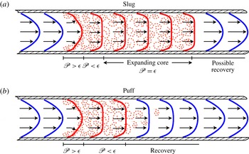
I will begin with the slug and restate in slightly more detail what was previously discussed concerning figures 5 and 6. Consider the schematic slug in figure 16(a), illustrating both the turbulent fluctuations and the mean shear profile. The vertical scale is greatly expanded. Upstream of the slug, the flow is fully developed laminar flow. Crossing the upstream interface, there is a rapid, almost explosive conversion of kinetic energy from the faster-moving laminar upstream flow into turbulence. In the vicinity of the upstream interface, there is a region of several pipe diameters in streamwise extent where the mean profile is highly distorted and turbulent production is very high. The cross-sectionally integrated production significantly exceeds the integrated dissipation (Wygnanski & Champagne Reference Wygnanski and Champagne1973; Song et al. Reference Song, Barkley, Avila and Hof2016).
Sketches illustrating the essential mechanics of (a) slugs and (b) puffs. The vertical scale is highly stretched. Turbulent flow is indicated by red dashed shading. Laminar velocity profiles are shown in blue while turbulent mean profiles are shown in red. The relative size of the integrated turbulent energy production
 $\mathscr{P}$
and dissipation
 $\unicode[STIX]{x1D716}$
in various regions is indicated.

It takes some time (that is, downstream distance) for the turbulent cascade to set in, for Reynolds stresses to act, and for the mean shear profile to adjust to a blunted turbulent shear profile. There is a region downstream of the interface where the integrated production falls below the integrated dissipation (Song et al. Reference Song, Barkley, Avila and Hof2016). Only at a distance on the order of 8 diameters from the interface, does the flow come into equilibrium and form the core of the slug. In this core region, the integrated production and dissipation are in balance. The slug is an expanding turbulent structure. In the absence of end effects, the core of a slug can be arbitrarily long, and it forms the axially and azimuthally statistically invariant state of fully developed turbulent pipe flow (Pope Reference Pope2000).
Slugs also have a downstream interface between turbulent and laminar flow. The situation at the downstream interface depends on the Reynolds number (Duguet et al.
Reference Duguet, Willis and Kerswell2010; Barkley et al.
Reference Barkley, Song, Mukund, Lemoult, Avila and Hof2015; Song et al.
Reference Song, Barkley, Avila and Hof2016). Essentially, there are two possibilities, corresponding to the two cases already discussed. At high
 $Re$
, turbulence invades the downstream laminar flow at the downstream front, whereas at lower
 $Re$
, turbulence undergoes a reverse transition to laminar flow at the downstream front. I will delay a detailed discussion of the downstream front until later, primarily because nothing that happens there is an input to the theory. Rather, the behaviour at the downstream front arises as a natural output from the theory.
7.2 Puffs
To explain the essential physics of a puff, I will take a slightly unusual approach. Consider what would be expected to occur to a slug as the Reynolds number of the flow is decreased (the viscosity is increased). It is sure that, eventually, production within the core of the slug will be unable to compensate the increased dissipation due to increased viscosity. The core of a slug will not be sustained. It is not essential exactly how it occurs, only that necessarily it must occur with decreasing
 $Re$
. Even with the collapse of the core, there will still be an upstream interface. While this interface is affected to some extent by the decrease in
 $Re$
, we started this thought experiment from a slug state in which production exceeds dissipation in the interface region, hence we would not expect the upstream interface to vanish simultaneously with the core. In fact it does not, it leads to a puff.
The above hopefully gives a sense of why puffs naturally follow from slugs as the Reynolds number is decreased. Given the structure of the slug in figure 16(a), the puff in figure 16(b) follows naturally as the turbulent core is lost due to increased dissipation. The above also provides intuition for the well-established fact that we will see in depth shortly: there is a smooth evolution of the upstream front with Reynolds number going between puffs and slugs. This is not the case for the downstream front.
It is useful to consider the structure of a puff from a more standard perspective. Wygnanski & Champagne (Reference Wygnanski and Champagne1973), Darbyshire & Mullin (Reference Darbyshire and Mullin1995), Shimizu & Kida (Reference Shimizu and Kida2009), Hof et al. (Reference Hof, de Lozar, Avila, Tu and Schneider2010) and many others discuss the fluid mechanics of puffs in some detail. A near-perfect description for my purposes is given in van Doorne & Westerweel (Reference van Doorne and Westerweel2009), so I refer the reader to my sketch in figure 16(b) while quoting van Doorne & Westerweel: ‘The fluid that enters the turbulent region with a high velocity at the upstream end of the puff thus provides the necessary energy to sustain the turbulent motions inside the puff. This energy is quickly converted into turbulent motions and dissipated, which results in an almost uniform velocity profile at the downstream end of the puff. The hairpin vortices that pass this (moving) plane decay quickly, because it is no longer possible to extract energy from a uniform flow; the flow then relaminarizes, and further downstream, the wall shear layers develop and the centreline velocity again increases.’ Notice that, for a puff, no parcels of fluid remain in the turbulent state. Puff turbulence is sustained only by continually entraining fresh laminar fluid at the upstream front (which, I add, is exactly how action potentials sustain themselves, by continually exciting quiescent parts of the medium).
There is one final crucial point. A puff consists not only of a localized patch of turbulence, but also of a downstream refractory region in which turbulence cannot be re-excited (van Doorne & Westerweel Reference van Doorne and Westerweel2009; Hof et al. Reference Hof, de Lozar, Avila, Tu and Schneider2010; Samanta et al. Reference Samanta, De Lozar and Hof2011). As the final part of previous quote indicates, the refractory region is an integral part of what a puff is. It must exist, or else the turbulence would not be localized; it would expand downstream. The refractory region was already shown in figure 15, as well as in figure 16(b). In the recovery region, the flow near the pipe centre accelerates, and the shear profile recovers its parabolic form. Turbulence cannot be excited downstream until the flow has at least mostly recovered. It is useful to consider a pair of puffs (e.g. Hof et al. Reference Hof, de Lozar, Avila, Tu and Schneider2010). A downstream puff cannot survive too close to an upstream puff because there is not sufficient energy in the blunted downstream velocity profile. Either the downstream puff will dissipate, or it will move to increase the distance from the upstream puff. Thus, the refractory region sets an interaction distance, typically of about the same size as the turbulent region itself. Slugs at the lowest Reynolds numbers for which they exist also have similar refractory regions (Song et al. Reference Song, Barkley, Avila and Hof2016). Slugs at high Reynolds numbers do not.
Needless to say there is much, much more that could be said about the fluid mechanics of puffs and slugs. Yet, the simple mechanisms that I have just described, together with the fluctuations intrinsic to turbulent flow, are the essential ingredients driving nearly all the large-scale dynamics of transitional turbulent pipe flow.
8 A better theory
I will now describe a theory that incorporates the known physics of shear flows and that naturally accounts for localized puffs as intermediary states on the route from laminar flow to expanding turbulence (Barkley Reference Barkley2011a
). The idea is simple. To the previous model involving only the turbulence level,
 $q(x,t)$
, a second variable,
 $u(x,t)$
, is added which represents the state of the mean shear and accounts for the effect of the mean shear on the turbulence, and vice versa. An important benefit of this additional variable is that it also allows a more realistic treatment of downstream advection (Barkley et al.
Reference Barkley, Song, Mukund, Lemoult, Avila and Hof2015). The model will no longer be variational. It will, however, effectively reduce to the previous case at sufficiently low and high Reynolds numbers.
8.1 The variable
 $u$

I want the new variable
 $u$
to be a scalar that encodes the state of the mean shear profile at each streamwise location
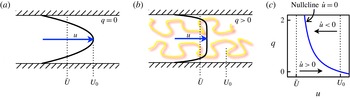
 $x$
. A nearly ideal choice is the mean streamwise velocity on the centreline. As illustrated in figure 17(a,b), this velocity component is largest when the flow is fully recovered laminar flow, and it is reduced for a blunted, turbulent shear profile. As already indicated in figure 16, shear profiles exhibit complex forms in the interface regions between turbulent and laminar flow (e.g. Wygnanski & Champagne Reference Wygnanski and Champagne1973; Hof et al.
Reference Hof, de Lozar, Avila, Tu and Schneider2010). Nevertheless, the centreline velocity captures, as well as one could hope with a single scalar quantity, the state of the streamwise shear profile. I will refer to
 $u$
sometimes as centreline velocity (dropping the mean and streamwise qualifiers) and sometimes as the mean shear, since this is the more relevant physical feature that it is meant to represent.
Dynamics of the variable
 $u$
. (a) In the absence of turbulence,
 $u$
will equilibrate at the laminar centreline velocity
 $U_{0}$
. (b) In the presence of turbulence, the mean velocity profile is blunted and
 $u$
will equilibrate at a value slightly larger than the bulk velocity
 $\bar{U}$
. (c) Nullcline diagram in the local phase plane, illustrating the dynamics of
 $u$
for fixed value of
 $q$
.

To arrive at the evolution of the variable
 $u$
, it is reasonable to start from the streamwise component of Reynolds averaged Navier–Stokes equations for a non-swirling, statistically axisymmetric flow (Pope Reference Pope2000),
 $$\begin{eqnarray}\frac{\unicode[STIX]{x2202}U_{x}}{\unicode[STIX]{x2202}t}+U_{x}\frac{\unicode[STIX]{x2202}U_{x}}{\unicode[STIX]{x2202}x}+U_{r}\frac{\unicode[STIX]{x2202}U_{x}}{\unicode[STIX]{x2202}r}=-\frac{\unicode[STIX]{x2202}P}{\unicode[STIX]{x2202}x}+\unicode[STIX]{x1D708}\left(\frac{\unicode[STIX]{x2202}^{2}U_{x}}{\unicode[STIX]{x2202}x^{2}}+\frac{1}{r}\frac{\unicode[STIX]{x2202}}{\unicode[STIX]{x2202}r}\left(r\frac{\unicode[STIX]{x2202}U_{x}}{\unicode[STIX]{x2202}r}\right)\right)+F_{x},\end{eqnarray}$$
where
 $U_{x}$
and
 $U_{r}$
are the mean streamwise and wall-normal velocities, and
 $P$
is the mean pressure.
 $F_{x}$
is the streamwise force component generated by Reynolds stresses.
On the centreline,
 $r=0$
,
 $$\begin{eqnarray}U_{r}(r=0)=\left.\frac{\unicode[STIX]{x2202}U_{x}}{\unicode[STIX]{x2202}r}\right|_{r=0}=0,\quad \left.\frac{1}{r}\frac{\unicode[STIX]{x2202}}{\unicode[STIX]{x2202}r}\left(r\frac{\unicode[STIX]{x2202}U_{x}}{\unicode[STIX]{x2202}r}\right)\right|_{r=0}=2\left.\frac{\unicode[STIX]{x2202}^{2}U_{x}}{\unicode[STIX]{x2202}r^{2}}\right|_{r=0},\end{eqnarray}$$
so that (8.1) on the centreline is
 $$\begin{eqnarray}\frac{\unicode[STIX]{x2202}U_{x}}{\unicode[STIX]{x2202}t}+U_{x}\frac{\unicode[STIX]{x2202}U_{x}}{\unicode[STIX]{x2202}x}=\left(-\frac{\unicode[STIX]{x2202}P}{\unicode[STIX]{x2202}x}+2\unicode[STIX]{x1D708}\frac{\unicode[STIX]{x2202}^{2}U_{x}}{\unicode[STIX]{x2202}r^{2}}+F_{x}\right)+\unicode[STIX]{x1D708}\frac{\unicode[STIX]{x2202}^{2}U_{x}}{\unicode[STIX]{x2202}x^{2}}.\end{eqnarray}$$
While an exact statement, (8.3) is not closed, because the terms contained within parentheses on the right-hand side are not determined by the centreline velocity alone. With or without turbulence, the centreline velocity is determined by the full profile, from the pipe wall to the centre, again reflecting that the actual variable is the shear profile, for which the centreline velocity is only a proxy.
Nevertheless, it is straightforward to close the centreline equation by modelling the cases where there is no turbulence, figure 17(a), and where there is turbulence, figure 17(b). Both cases are relatively simple and well understood. Take the equation for
 $u(x,t)$
to be
 $$\begin{eqnarray}\frac{\unicode[STIX]{x2202}u}{\unicode[STIX]{x2202}t}+u\frac{\unicode[STIX]{x2202}u}{\unicode[STIX]{x2202}x}=g(q,u)+\unicode[STIX]{x1D708}\frac{\unicode[STIX]{x2202}^{2}u}{\unicode[STIX]{x2202}x^{2}},\end{eqnarray}$$
where
 $q$
is the turbulence level and
 $g(q,u)$
is to be chosen to mimic the effects of omitted terms.
To determine a reasonable form for
 $g(q,u)$
, consider streamwise-invariant cases in which
 $q$
takes specified fixed values. Streamwise invariance reduces the
 $u$
dynamics to
 $$\begin{eqnarray}\dot{u}=g(q,u),\end{eqnarray}$$
which is the equation for the local dynamics of
 $u$
.
Without turbulence, i.e.
 $q=0$
as in figure 17(a), we know that whatever the state of the initial profile, the flow will accelerate under imposed pressure gradient until the viscous stresses balance the pressure gradient, at which point the velocity profile will be the fully developed parabolic Hagen–Poiseuille flow with a centreline speed denoted by
 $U_{0}$
. (See Narasimha & Sreenivasan (Reference Narasimha and Sreenivasan1979) for a discussion of the approach to laminar flow following relaminarization.) We know from a leading-order Taylor expansion that the final stage of this relaxation will be linear decay, and so of the form
 $$\begin{eqnarray}\dot{u}=\unicode[STIX]{x1D716}_{1}(U_{0}-u),\end{eqnarray}$$
where
 $\unicode[STIX]{x1D716}_{1}$
is a relaxation rate. The relaxation time will be of the order of the viscous time scale
 $d^{2}/\unicode[STIX]{x1D708}$
, and hence in non-dimensional form the relaxation rate will be of the order
 $Re^{-1}$
. One could in principle numerically obtain this rate directly from the Navier–Stokes equation (e.g. Meseguer & Trefethen Reference Meseguer and Trefethen2003). In the interest of simplicity, here I will take
 $\unicode[STIX]{x1D716}_{1}$
to be a fixed model parameter. Thus, while the actual evolution of the centreline velocity to the laminar equilibrium is more complicated than described by (8.6), this form gives a simple, qualitatively reasonable approximation for the dynamics of
 $u$
in the absence of turbulence.
Now consider the dynamics of
 $u$
in the presence of a fixed level of turbulence, as in figure 17(b). Reynolds stresses will now play a significant role in counter-balancing the pressure gradient, and the centreline velocity will be reduced from the value
 $U_{0}$
, but it will be limited by the value of the bulk velocity
 $\bar{U}$
. This suggests a model of the form
 $$\begin{eqnarray}\dot{u}=g(q,u)=\unicode[STIX]{x1D716}_{1}(U_{0}-u)+\unicode[STIX]{x1D716}_{2}(\bar{U}-u)q,\end{eqnarray}$$
with
 $\unicode[STIX]{x1D716}_{2}$
a parameter giving the rate of decrease of
 $u$
in the presence of turbulence. In the limit of large
 $q$
, (8.7) will evolve to give
 $u\simeq \bar{U}$
. It can be argued that one should have a factor
 $q^{2}$
rather than
 $q$
in the last term. In practice I have not found it to make much difference to the overall dynamics of the model, and since the model was originally written with a factor
 $q$
(Barkley Reference Barkley2011a
), I will continue to use it here.
Nullclines are curves in the
 $(u,q)$
phase plane on which time derivatives of variables in the local dynamics is zero. The
 $u$
-nullcline is given by
 $\dot{u}=0$
, that is
 $g(q,u)=0$
. This can be written
 $$\begin{eqnarray}q=\frac{\unicode[STIX]{x1D716}_{1}(U_{0}-u)}{\unicode[STIX]{x1D716}_{2}(\bar{U}-u)},\end{eqnarray}$$
and is shown in figure 17(c). Off the nullcline, the time derivative of
 $u$
is non-zero. Horizontal arrows indicate the evolution of
 $u$
towards the
 $u$
-nullcline for fixed
 $q$
. One can see graphically that, for
 $q=0$
,
 $u$
will evolve to
 $U_{0}$
. With fixed, non-zero
 $q$
,
 $u$
will tend towards a value slightly larger than
 $\bar{U}$
.
Adding back the space-dependent terms, the model equation for
 $u$
is
 $$\begin{eqnarray}\frac{\unicode[STIX]{x2202}u}{\unicode[STIX]{x2202}t}+u\frac{\unicode[STIX]{x2202}u}{\unicode[STIX]{x2202}x}=\unicode[STIX]{x1D716}_{1}(U_{0}-u)+\unicode[STIX]{x1D716}_{2}(\bar{U}-u)q+\unicode[STIX]{x1D708}\frac{\unicode[STIX]{x2202}^{2}u}{\unicode[STIX]{x2202}x^{2}}.\end{eqnarray}$$
Let me comment on
 $U_{0}$
and
 $\bar{U}$
. I have left these as parameters in the model for two reasons. The first is that if one wanted to consider a related flow, such as flow in a square or rectangular duct, then the numerical values of
 $U_{0}$
and
 $\bar{U}$
would be different from those of pipe flow. It is therefore desirable to have these values identified explicitly in the model equations. The second, more important reason has to do with frames of reference. By including these velocities as parameters, I can effectively capture Galilean invariance with the model. As we have seen, there are two reference frames that are natural when considering pipe flow – the laboratory frame, in which the pipe is stationary, and the frame moving at the bulk velocity. I want the model to be equally valid in either reference frame, or any other. As written, one need only specify the values of
 $U_{0}$
and
 $\bar{U}$
appropriate to a particular frame of reference of interest for
 $u$
to be relative to that frame of reference.
8.2
$q$
dynamics

For the evolution of the turbulent field,
 $q$
, I need to account for the negative feedback of the mean shear, but otherwise I want to make minimal modifications to the local dynamics presented in § 4. The simplest thing to do is to use the same dynamics for
 $q$
as in (4.3) when the shear profile is fully recovered,
 $u=U_{0}$
, but inhibit the growth of turbulence for
 $u<U_{0}$
to take into account the reduced turbulent production for a blunted shear profile (Pope Reference Pope2000).
I propose simply to extend the local
 $q$
dynamics given by (4.3) to
 $$\begin{eqnarray}\dot{q}=f(q,u)=q[r+(u-U_{0})-(r+\unicode[STIX]{x1D6FF})(q-1)^{2}].\end{eqnarray}$$
When the shear profile is fully recovered,
 $u=U_{0}$
, this reduces to the previous form. (See appendix B for commentary on the function
 $f(q,u)$
.)
To visualize the dynamics of
 $q$
, I again turn to nullclines, now the curves on which
 $\dot{q}=f(q,u)=0$
. Expressing
 $q$
as a function of
 $u$
, the
 $q$
-nullcline has three branches
 $$\begin{eqnarray}q=\left\{\begin{array}{@{}ll@{}}q^{+}(u)=1+\sqrt{{\displaystyle \frac{r+u-U_{0}}{r+\unicode[STIX]{x1D6FF}}}}\quad \quad & \text{(upper branch)},\\ q^{-}(u)=1-\sqrt{{\displaystyle \frac{r+u-U_{0}}{r+\unicode[STIX]{x1D6FF}}}}\quad \quad & \text{(lower branch)},\\ q^{0}(u)=0\quad & \text{(laminar)}.\end{array}\right.\end{eqnarray}$$
As we will see, the upper, lower and laminar branches of the
 $q$
-nullcline are intimately related to upper, lower and laminar steady states, and hence the same terminology is used for both. Figure 18(a) shows typical
 $q$
-nullclines. The
 $q$
dynamics, with
 $u$
held fixed, is indicated by vertical arrows. The upper and laminar branches are attractive, while the lower branch is repelling. The lower branch thus sets the nonlinear threshold for transition to the upper branch. As can be seen, the threshold increases as
 $u$
decreases; that is, triggering turbulence from a blunted profile is more difficult than from fully recovered flow. The upper and lower branches are part of a single parabolic curve that has its nose at
 $q=1$
,
 $u^{\ast }=U_{0}-r$
. Hence as
 $r$
increases,
 $u^{\ast }$
decreases, as is seen in figure 18(b), to be discussed in detail momentarily.
Before putting the
 $q$
and
 $u$
dynamics together, I need to address the spatial variation of
 $q$
. Again, I will make only minimal changes to the simple model (4.5). The only change will be in the advection term. Previously, the downstream advection was a specified constant
 $U$
. Now, having a variable
 $u$
representing the streamwise velocity on the centreline, I can use this variable to set the downstream advection of
 $q$
. I will take
 $q(x,t)$
to be governed by
 $$\begin{eqnarray}\frac{\unicode[STIX]{x2202}q}{\unicode[STIX]{x2202}t}+(u-\unicode[STIX]{x1D701})\frac{\unicode[STIX]{x2202}q}{\unicode[STIX]{x2202}x}=f(q,u)+D\frac{\unicode[STIX]{x2202}^{2}q}{\unicode[STIX]{x2202}x^{2}},\end{eqnarray}$$
where
 $\unicode[STIX]{x1D701}$
is an additional parameter. The justification for using
 $u-\unicode[STIX]{x1D701}$
rather than
 $u$
for the advection speed is the following. Firstly,
 $u$
represents the maximum of the streamwise velocity profile, and it is not reasonable that turbulence is advected at this maximum speed. More importantly, numerical evidence shows that turbulence is advected at a speed smaller than the centreline speed by roughly a fixed constant throughout the transition regime (Song et al.
Reference Song, Barkley, Avila and Hof2016). While I would prefer not to introduce another parameter and a somewhat awkward term into the model, it is necessary to obtain correct behaviour and agreement with established facts.
The heart of the model as seen in the local phase plane. (a)
 $q$
-nullclines (red curves) for a representative value of
 $r$
. There are three branches: attracting laminar and upper branches,
 $q^{0}$
and
 $q^{+}$
, separated by a repelling lower branch
 $q^{-}$
. Branches
 $q^{+}$
and
 $q^{-}$
meet at
 $(q=1,u=u^{\ast })$
, as labelled. At
 $u=U_{0}$
the dynamics of
 $q$
is exactly as given by the one-variable model. (b) Nullclines for
 $q$
(red curves) and
 $u$
(blue curve) plotted together. Nullclines are shown for three values of
 $r$
(
 $0.3$
,
 $0.6$
and
 $0.9$
), illustrating the behaviour as
 $r$
increases. Fixed points at intersections of
 $q$
- and
 $u$
-nullclines are indicated by dots. The laminar fixed point
 $(q=0,u=U_{0})$
exists for all
 $r$
. As
 $r$
increases,
 $u^{\ast }$
decreases and a second pair of fixed points bifurcates. (c) Excitable dynamics at
 $r=0.6$
. The only fixed point is laminar flow. A trajectory shows typical evolution starting from an initial condition perturbed from laminar flow. (d) Bistable dynamics at
 $r=0.9$
. Starting from the same state as in (c), the trajectory evolves to the stable upper-branch equilibrium.

8.3 Heart of the model
The heart of the model is the local dynamics given by the pair of equations
 $$\begin{eqnarray}\dot{q}=f(q,u),\quad \dot{u}=g(q,u),\end{eqnarray}$$
where
 $f$
and
 $g$
are given in (8.10) and (8.7), respectively. These equations express the interplay between turbulence intensity and the mean shear profile in a small region of space, or equivalently when large-scale spatial variations are neglected. I refer the reader back to figure 7 and the discussion in § 4.1.
I have discussed separately the dynamics of each variable in terms of nullclines; now I will put the two together. Figure 18(b) shows nullclines for both
 $q$
and
 $u$
, for three values of
 $r$
. Only the upper and lower branches of the
 $q$
-nullcline depend on
 $r$
. Wherever nullclines intersect, the local dynamics has a fixed point:
 $\dot{q}=\dot{u}=0$
. There is a fixed point at
 $(q=0,u=U_{0})$
, corresponding to fully developed laminar flow, for all values of
 $r$
. This fixed point is always stable.
For small
 $r$
, the laminar fixed point is the only fixed point of the local dynamics. As
 $r$
increases, the nullclines intersect in two further fixed points, corresponding to upper (stable) and lower (unstable) branch turbulent states. The local dynamics is then bistable. While similar to the transition to bistability in the one-variable model, here the dynamics is significantly richer.
Figure 18(c,d) shows the qualitatively different phase portraits obtained from the model for values of
 $r$
below and above the onset of bistability. Let me first discuss the bistable case,
 $r=0.9$
, in figure 18(d). Shown is a trajectory starting away from the laminar fixed point with a small level of turbulence. The trajectory moves upwards under strong nonlinear amplification of
 $q$
, while
 $u$
initially decreases only slightly. The nonlinear amplification stops with
 $q$
saturating along the upper branch of the nullcline
 $q^{+}(u)$
. Subsequently, on a slower time scale, the shear profile
 $u$
adjusts in response to the increased turbulence level, and the trajectory eventually approaches the upper-branch fixed point. Here the turbulence level and shear profile are in equilibrium. This is the situation for the core of a turbulent slug where turbulent production in the presence of the blunted profile is sufficient to balance dissipation and an equilibrium is established.
Now consider the case for
 $r=0.6$
in figure 18(c). This is the excitable case. A trajectory is again shown starting away from the laminar fixed point. The trajectory moves to the upper branch of the
 $q$
-nullcline under nonlinear amplification of
 $q$
, and subsequently the shear profile
 $u$
adjusts in response. Now, however, no equilibrium can be established at this value of Reynolds number. Turbulent fluctuations cannot be maintained once the shear profile is blunted, and so turbulence drops. In the absence of turbulence, the profile
 $u$
then begins to recover its parabolic form. Initially, during this recovery, the threshold for re-excitation into turbulence is large (set by the lower branch
 $q^{-}$
), thereby making the system refractory. Eventually, the system returns to the laminar fixed point and the threshold is again small. Note, this is precisely what occurs in traversing a turbulent puff.
I end with the following thoughts on the local dynamics. On the one hand, the extension from the simple variational dynamics,
 $\dot{q}=-V^{\prime }(q)$
, is relatively minor. I added a reasonable second variable to account for the negative feedback of the mean shear on the turbulence. On the other hand, in the region where turbulence first arises, the effect of this second variable is profound. This is best seen in the direction of decreasing
 $r$
. When the upper equilibrium is lost, whether in the model or real turbulent flow, this does not immediately signal that turbulence cannot be temporarily excited. The equilibrium is only lost because turbulence cannot be maintained in the presence of a blunted shear profile. At least for some range of Reynolds numbers, turbulence can rapidly grow from a fully developed laminar profile even if ultimately it is not sustained. (I refer the reader back to figure 16 and the related discussion.)
8.4 Summary
For future reference, I here summarize the two-variable model as it will be studied in the remainder of the paper. The turbulence intensity
 $q(x,t)$
and mean shear
 $u(x,t)$
evolve according to the equations
 $$\begin{eqnarray}\displaystyle & \displaystyle \frac{\unicode[STIX]{x2202}q}{\unicode[STIX]{x2202}t}+(u-\unicode[STIX]{x1D701})\frac{\unicode[STIX]{x2202}q}{\unicode[STIX]{x2202}x}=f(q,u)+D\frac{\unicode[STIX]{x2202}^{2}q}{\unicode[STIX]{x2202}x^{2}}+\unicode[STIX]{x1D70E}q\unicode[STIX]{x1D702}, & \displaystyle\end{eqnarray}$$
 $$\begin{eqnarray}\displaystyle & \displaystyle \frac{\unicode[STIX]{x2202}u}{\unicode[STIX]{x2202}t}+u\frac{\unicode[STIX]{x2202}u}{\unicode[STIX]{x2202}x}=g(q,u), & \displaystyle\end{eqnarray}$$
where the functions
 $f(q,u)$
and
 $g(q,u)$
describing the local dynamics are given by
 $$\begin{eqnarray}\displaystyle & \displaystyle f(q,u)=q(r+u-U_{0}-(r+\unicode[STIX]{x1D6FF})(q-1)^{2}), & \displaystyle\end{eqnarray}$$
 $$\begin{eqnarray}\displaystyle & \displaystyle g(q,u)=\unicode[STIX]{x1D716}_{1}(U_{0}-u)+\unicode[STIX]{x1D716}_{2}(\bar{U}-u)q. & \displaystyle\end{eqnarray}$$
I have included a multiplicative noise term in the equation for the
 $q$
dynamics, even though for the much of the analysis I will set the noise strength
 $\unicode[STIX]{x1D70E}$
to zero. The reader will also observe that I have dropped the diffusive term from the
 $u$
dynamics. This is equivalent to making the boundary-layer approximation. Had I made the boundary-layer approximation at the outset in deducing (8.14b
), this diffusive term would not appear. I have not found that it affects the dynamics one way or the other, and so for simplicity it will not be included.
In Barkley et al. (Reference Barkley, Song, Mukund, Lemoult, Avila and Hof2015) it is shown that model parameters can be adjusted to match, quantitatively, front speeds of both pipe and duct flow. There is a lengthy discussion there about the fitting procedure. I will not be fitting experimental data here, and I therefore choose instead to fix parameters at simple, representative values. Unless stated otherwise, the model parameters will be set to the following values:
 $$\begin{eqnarray}\displaystyle \unicode[STIX]{x1D701}=0.8,\quad D=0.5,\quad \unicode[STIX]{x1D6FF}=0.1,\quad \unicode[STIX]{x1D716}_{1}=0.1,\quad \unicode[STIX]{x1D716}_{2}=0.2. & & \displaystyle\end{eqnarray}$$
When the noise term is included, I will normally use
 $$\begin{eqnarray}\displaystyle \unicode[STIX]{x1D70E}=0.5. & & \displaystyle\end{eqnarray}$$
These have been determined by the desire to use simple values while achieving model dynamics that closely mimics actual pipe flow. The overall dynamics of the model are, however, very robust to changes in parameter values. See appendix B for some commentary on this and other models, as well as numerical details.
9 Deterministic dynamics
In this section I will analyse the model dynamics in depth, and relate these dynamics to observed behaviour in pipe flow. I consider only deterministic dynamics, and leave treatment of fluctuations to the next section.
9.1 The basics
Let us first recall the situation for the one-variable model shown in figure 10. The key point there was the crossing of the upstream and downstream front speeds. Below the crossing point, turbulent patches shrink or decay, and the flow is asymptotically laminar. Above the crossing point, turbulent patches invade laminar flow in the form of turbulent slugs.
Figure 19 shows how this picture is modified when the effect of the mean shear is included. Now stable, localized states exist between expanding and decaying turbulence. There is still a crossing point of upstream and downstream front speeds leading to expanding turbulence. However, below the crossing point, turbulence does not contract to zero, but instead persists in localized form. The branch of localized states ends in a saddle-node bifurcation with a branch of unstable localized states (dashed curve) consisting of edge states separating laminar and turbulent flow. For
 $r$
below the saddle-node bifurcation, turbulence inevitably decays.
This diagram is going to occupy us for much of the remainder of the paper. However, before diving into details, I want to give a brief overview of puff and slug states.
Dynamics of the two-variable model. The upper plot (a) shows speeds of upstream and downstream fronts as a function of model Reynolds number
 $r$
. Below are space–time plots of turbulent intensity
 $q$
at representative values of
 $r$
: (b)
 $r=0.3$
, (c)
 $r=0.6$
and (d)
 $r=0.9$
. Between decaying turbulence in region I and expanding turbulence in region III, there is a region, region II, of persistent localized states (puffs). Compare with figure 10 for the one-variable model. The dashed curve in (a) indicates a branch of unstable localized states (edge states) that meets the stable puff branch in a saddle-node bifurcation. The three space–time plots start from the same initial condition (localized puff solution). The time scale for (b) is 20 times shorter than for (c) and (d).

Puffs and slugs in the two-variable model. States are shown in physical space in panels (a,c,e) and in the local phase plane in panels (b,d,f). Arrows in the phase plane indicate increasing streamwise coordinate,
 $x$
, not time. Nullclines for
 $q$
(red) and
 $u$
(blue) are shown in the phase plane. (a,b) Puff at
 $r=0.6$
, as in figure 19(c). The local dynamics is excitable. (c,d) Slug at
 $r=0.9$
, as in figure 19(d). The local dynamics is bistable. The downstream front is a transition from turbulent to laminar flow, and is referred to as a weak downstream front. (e,f) Slug at
 $r=1.8$
. The local dynamics is bistable. At the downstream front the transition is from laminar to turbulent. This is referred to as a strong downstream front.

Figure 20 illustrates a typical puff and two slugs. The puff is the same state as shown in the space–time plot of figure 19(c). The first slug, figure 20(c,d), is the same state as shown in the space–time plot of figure 19(d). This slug is observed just after the onset of expansion. The second slug, figure 20(e,f), occurs for a larger value of
 $r$
.
Consider the three turbulent structures from upstream to downstream. All three upstream fronts are similar. (This is directly related to the smooth dependence of the upstream front speed on
 $r$
seen in figure 19.) At the upstream fronts,
 $q$
increases sharply in space, and the system moves towards the upper branch of the nullcline in the local phase plane. This corresponds to a rapid conversion of laminar flow to turbulent flow. In response there is a decrease in
 $u$
, corresponding to a blunting of the shear profile. At this point there is a distinction between the states.
For the puff, the local dynamics is excitable, figure 20(b), and there is no turbulent fixed point, meaning that it is not possible for the turbulent flow to persist in the presence of the modified shear. Hence, once the system approaches the nose of the
 $q$
-nullcline, the flow undergoes a reverse transition from turbulent to laminar flow. This is then followed by a slow recovery of the shear profile back to the fully recovered laminar state. The downstream front is always a fixed distance from the upstream front, determined by how long it takes the system to move along the upper branch of the
 $q$
-nullcline. The downstream front is slaved to the upstream front, and the fronts move at the same speed.
For slugs, the local dynamics has a stable upper-branch fixed point corresponding to the turbulent core of a slug, figure 20(d,f). The two slugs shown differ in their downstream fronts. For the case in figure 20(c,d), there is a reverse transition to laminar flow at the downstream front. This is called a weak downstream front and the slug is called a weak slug (Barkley et al. Reference Barkley, Song, Mukund, Lemoult, Avila and Hof2015). The weak front is not very different from the downstream front of a puff. The speed of this front differs from the speed of the upstream front, and hence the slug expands, as seen in the space–time plot in figure 19. I want to stress, however, that all of the increase in turbulence occurs at the upstream front, where laminar flow becomes turbulent. At the downstream front, there is a reverse transition from turbulent to laminar flow. I will return to this important point shortly.
For the slug shown in figure 20(e,f), the downstream front is much like the upstream front. This is called a strong downstream front and the slug is called a strong slug (Barkley et al.
Reference Barkley, Song, Mukund, Lemoult, Avila and Hof2015). Laminar flow is transitioning to turbulent flow on both ends of the slug. The upstream and downstream speeds are nearly symmetrical with respect to the bulk speed
 $\bar{U}$
. Turbulence expands rapidly in this case. One can see in figure 19 that there is a continuous variation in the speed of the downstream front, and hence a continuous transition between the two types of slugs. (See also Duguet et al. (Reference Duguet, Willis and Kerswell2010) for comments on the two types of slugs, and Nishi et al. (Reference Nishi, Ünsal, Durst and Biswas2008), Song et al. (Reference Song, Barkley, Avila and Hof2016) for experiments and simulations showing two types of slugs.)
The basic distinction between puffs and slugs follows just from the distinction between excitable and bistable dynamics. However, to fully understand how puffs are localized, how they delocalize to form slugs, and what distinguishes the two types of slugs, we need to study fronts in more detail.
9.2 Singular perturbation analysis
I now begin a rather lengthy analysis of travelling fronts using a standard singular perturbation analysis (Rinzel & Terman Reference Rinzel and Terman1982; Tyson & Keener Reference Tyson and Keener1988; Keener & Sneyd Reference Keener and Sneyd2008). The main point of this analysis is not to obtain approximate solutions to the nonlinear partial differential equations. Rather, it is the simplification it brings into the basic mechanism for puffs, slugs, and other features of transitional flow. By its very nature, the approach cleanly separates the interfaces, where the turbulence intensity changes on fast scales, from other regions.
The idea behind the approach is the following. We have already seen that the dynamics is dominated by rapid transitions between the stable branches of the
 $q$
-nullcline and subsequent slower evolution of
 $u$
. The difference in time scales between
 $q$
and
 $u$
is dictated by the small parameters
 $\unicode[STIX]{x1D716}_{1}$
and
 $\unicode[STIX]{x1D716}_{2}$
appearing in
 $g(q,u)$
, the function modelling the local
 $u$
dynamics (8.14d
). In the perturbation analysis, the time scale separation is made artificially large by sending these parameters towards zero.
The analysis is most simply done by expressing the two parameters,
 $\unicode[STIX]{x1D716}_{1}$
and
 $\unicode[STIX]{x1D716}_{2}$
, in terms of a single parameter,
 $\unicode[STIX]{x1D716}$
, via
 $$\begin{eqnarray}\unicode[STIX]{x1D716}_{1}=\unicode[STIX]{x1D716},\quad \unicode[STIX]{x1D716}_{2}=\unicode[STIX]{x1D705}\unicode[STIX]{x1D716},\end{eqnarray}$$
where is
 $\unicode[STIX]{x1D705}$
is a fixed value. The standard values of
 $\unicode[STIX]{x1D716}_{1}$
and
 $\unicode[STIX]{x1D716}_{2}$
in (8.15) correspond to
 $\unicode[STIX]{x1D705}=2$
. Then define
 $G(q,u)$
via
 $$\begin{eqnarray}g(q,u)=\unicode[STIX]{x1D716}G(q,u)=\unicode[STIX]{x1D716}\{(U_{0}-u)+\unicode[STIX]{x1D705}(\bar{U}-u)q\}.\end{eqnarray}$$
In terms of
 $\unicode[STIX]{x1D716}$
and
 $G(q,u)$
, the model reads
 $$\begin{eqnarray}\displaystyle & \displaystyle \frac{\unicode[STIX]{x2202}q}{\unicode[STIX]{x2202}t}+(u-\unicode[STIX]{x1D701})\frac{\unicode[STIX]{x2202}q}{\unicode[STIX]{x2202}x}=f(q,u)+D\frac{\unicode[STIX]{x2202}^{2}q}{\unicode[STIX]{x2202}x^{2}}, & \displaystyle\end{eqnarray}$$
 $$\begin{eqnarray}\displaystyle & \displaystyle \frac{\unicode[STIX]{x2202}u}{\unicode[STIX]{x2202}t}+u\frac{\unicode[STIX]{x2202}u}{\unicode[STIX]{x2202}x}=\unicode[STIX]{x1D716}G(q,u). & \displaystyle\end{eqnarray}$$
Consider a front solution after initial transients have died down so that the front is travelling at constant speed
 $c$
. Make a coordinate transformation to go into a co-moving frame of reference,
 $z=x-ct$
, and locate the now stationary front at
 $z=0$
. The steady front satisfies
 $$\begin{eqnarray}\displaystyle & \displaystyle (u-\unicode[STIX]{x1D701}-c)\frac{\text{d}q}{\text{d}z}=f(q,u)+D\frac{\text{d}^{2}q}{\text{d}z^{2}}, & \displaystyle\end{eqnarray}$$
 $$\begin{eqnarray}\displaystyle & \displaystyle (u-c)\frac{\text{d}u}{\text{d}z}=\unicode[STIX]{x1D716}G(q,u). & \displaystyle\end{eqnarray}$$
We need to consider the problem on two scales – the slow, or outer scale, and the fast, or inner scale. Changing momentarily to the slow space scale
 $\tilde{z}=\unicode[STIX]{x1D716}z$
, the equations for the steady front on the outer scale become
 $$\begin{eqnarray}\displaystyle & \displaystyle \unicode[STIX]{x1D716}(u-\unicode[STIX]{x1D701}-c)\frac{\text{d}q}{\text{d}\tilde{z}}=f(q,u)+\unicode[STIX]{x1D716}^{2}D\frac{\text{d}^{2}q}{\text{d}\tilde{z}^{2}}, & \displaystyle\end{eqnarray}$$
 $$\begin{eqnarray}\displaystyle & \displaystyle \unicode[STIX]{x1D716}(u-c)\frac{\text{d}u}{\text{d}\tilde{z}}=\unicode[STIX]{x1D716}G(q,u). & \displaystyle\end{eqnarray}$$
 $\unicode[STIX]{x1D716}\rightarrow 0$
, we obtain
 $$\begin{eqnarray}\displaystyle & \displaystyle f(q,u)=0, & \displaystyle\end{eqnarray}$$
 $$\begin{eqnarray}\displaystyle & \displaystyle (u-c)\frac{\text{d}u}{\text{d}\tilde{z}}=G(q,u). & \displaystyle\end{eqnarray}$$
 $(q,u)$
must be a root of
 $f$
. That is, the system must be on one of the branches of the
 $q$
-nullcline. Only the stable branches are relevant. This means that, given
 $u$
,
 $q$
must be one of
 $$\begin{eqnarray}\displaystyle q=\left\{\begin{array}{@{}ll@{}}q^{+}(u)=1+\sqrt{{\displaystyle \frac{r+u-U_{0}}{r+\unicode[STIX]{x1D6FF}}}}\quad & \text{(upper branch)},\\ q^{0}(u)=0\quad & \text{(laminar)}.\end{array}\right. & & \displaystyle\end{eqnarray}$$
When viewed on the outer scale, fronts are discontinuous jumps between the stable branches of
 $f$
. See figure 21(a,b). Excluding the discontinuous jumps, the system is either on the
 $q^{+}$
- or
 $q^{0}$
-nullcline, and hence
 $q$
is a known function of
 $u$
. Denote this
 $q^{+/0}(u)$
. Then in the outer regions,
 $q$
can be eliminated in (9.6b
) to give
 $$\begin{eqnarray}(u-c)\frac{\text{d}u}{\text{d}\tilde{z}}=G(q^{+/0}(u),u).\end{eqnarray}$$
In principle, this equation can be solved for
 $u(\tilde{z})$
. In practice, we will not need to solve explicitly the outer equation, although some knowledge of the behaviour of the outer solutions will be needed.
Illustrative downstream front as seen on outer and inner scales. The front on the outer scale in the local phase plane (a) and in physical space (b). Arrows in (a) indicate increasing
 $\tilde{z}$
, the streamwise coordinate rescaled to outer units. The double arrow indicates the jumps between stable branches of the
 $q$
-nullcline, which are discontinuities on the outer scale. (c) The same front on the inner scale. Here
 $u=u_{f}$
is constant and
 $q$
is a smooth function of the stretched inner coordinate
 $\unicode[STIX]{x1D709}$
. The front speed is dictated by the inner solution.

Our main concern is with the fronts where the system jumps between stable branches of the
 $q$
-nullclines. At these jumps, derivatives are large, and so the limit we took in going from (9.5) to (9.6) is not valid. To analyse the jumps we use the fast, inner scaling and follow a similar procedure to that used in § 4.2.
Starting from (9.4), make a coordinate change to natural inner coordinate for the front
 $$\begin{eqnarray}\unicode[STIX]{x1D709}=\frac{z}{\sqrt{D}},\end{eqnarray}$$
and define
 $$\begin{eqnarray}s\equiv \frac{c-u+\unicode[STIX]{x1D701}}{\sqrt{D}}.\end{eqnarray}$$
Then the equations on the inner scale are
 $$\begin{eqnarray}\displaystyle & \displaystyle q^{\prime \prime }+sq^{\prime }+f(q,u)=0, & \displaystyle\end{eqnarray}$$
 $$\begin{eqnarray}\displaystyle & \displaystyle (u-c)u^{\prime }=\unicode[STIX]{x1D716}\sqrt{D}G(q,u), & \displaystyle\end{eqnarray}$$
 $\text{d}/\text{d}\unicode[STIX]{x1D709}$
. In the limit
 $\unicode[STIX]{x1D716}\rightarrow 0$
, the
 $u$
equation gives
 $$\begin{eqnarray}(u-c)u^{\prime }=0.\end{eqnarray}$$
This implies that, on the inner scale,
 $u$
is constant across a front. Call this constant value
 $u_{f}$
. Then, at leading order, the equations for a front on the inner scale become simply
 $$\begin{eqnarray}\displaystyle & \displaystyle q^{\prime \prime }+sq^{\prime }+f(q,u)=0, & \displaystyle\end{eqnarray}$$
 $$\begin{eqnarray}\displaystyle & \displaystyle u=u_{f}. & \displaystyle\end{eqnarray}$$
 $\unicode[STIX]{x1D709}\rightarrow \pm \infty$
are that the inner solution matches the outer solution on either side of the front. Namely, for a downstream front,
 $$\begin{eqnarray}q(-\infty )=q^{+}(u_{f}),\quad q(+\infty )=q^{0}.\end{eqnarray}$$
For an upstream front, the boundary conditions are reversed, but this is equivalent to keeping the same boundary conditions but changing the sign of
 $s$
in (9.13). Figure 21(c) shows a front on the inner scale.
Suppose for the moment that we know
 $u_{f}$
, then (9.13) together with boundary conditions (9.14) can be solved (numerically in practice) to give
 $q(\unicode[STIX]{x1D709})$
and the nonlinear eigenvalue
 $s$
. This is almost identical to the situation for the one-variable model, § 4.2, except here the value of
 $s$
will depend on
 $u_{f}$
as well as the parameter
 $r$
that appears in
 $f$
. Denote this dependence by
 $s(r,u_{f})$
. Then inverting (9.10) we obtain the leading-order asymptotic expressions for front speeds:
 $$\begin{eqnarray}\displaystyle & \displaystyle c_{u}=u_{f}-\unicode[STIX]{x1D701}-\sqrt{D}\,s(r,u_{f}), & \displaystyle\end{eqnarray}$$
 $$\begin{eqnarray}\displaystyle & \displaystyle c_{d}=u_{f}-\unicode[STIX]{x1D701}+\sqrt{D}\,s(r,u_{f}). & \displaystyle\end{eqnarray}$$
Note that the parameters
 $\unicode[STIX]{x1D716}_{1}$
and
 $\unicode[STIX]{x1D716}_{2}$
do not appear in (9.15), and hence they do not affect front speeds at leading order. Moreover, the diffusion term in (8.9) also would have not contributed to front speeds at leading order – a further justification for dropping this term from the model.
The advantage of having carried out the asymptotic analysis is that we see precisely what determines the front speeds. It is useful to compare (9.15) with similar expressions (4.13) for the one-variable model. (See also Holzner et al. (Reference Holzner, Song, Avila and Hof2013) and Song et al. (Reference Song, Barkley, Avila and Hof2016).) In both cases front speeds are determined by kinematic motion due to advection and by dynamical motion relative to the kinematic advection. For the one-variable model, the advection speed was a constant
 $U$
and the nonlinear eigenvalue
 $s$
was a function of model Reynolds number
 $r$
. Now we have additional dependence on
 $u_{f}$
, which is the essences of how speeds in the two models differ. Recall that, as discussed in § 8.1, the variable
 $u$
plays two related roles in the model. This is seen explicitly in the expressions for front speeds. In its role as centreline velocity,
 $u$
determines the local advection speed. In particular, at a front where
 $u=u_{f}$
, the turbulence intensity
 $q$
is advected at speed
 $u_{f}-\unicode[STIX]{x1D701}$
. (See the discussion following (8.12).) This is the kinematic component of front motion. In its role in encoding the state of the mean shear profile,
 $u$
plays a part in determining the dynamical component of the front speed via
 $s(r,u_{f})$
. Fronts occurring where the shear profile is blunted behave differently from those where the profile is fully recovered laminar flow. The values of
 $u_{f}$
will in general be different at upstream and downstream fronts, and these values must be determined in a global, self-consistent way, as I now explain.
9.3 Upstream front
The first step is to examine the upstream front, which as we have already seen is the same for puffs and slugs. The simplicity of the upstream front comes from the fact that it occurs directly from fully recovered Hagen–Poiseuille flow, and hence we know
 $u_{f}=U_{0}$
. It is not necessary to know anything further about the system to determine the shape and speed of this front. Figure 22(a,b) shows a typical upstream front. These plots include not just the inner-scale solution, the jump from
 $q^{0}$
to
 $q^{+}$
, but a portion of the surrounding outer-scale solution. Seen in physical space, figure 22(b), the upstream front always exhibits a characteristic overshoot in the turbulence intensity
 $q$
.
The expression for the upstream front speed is
 $$\begin{eqnarray}c_{u}=U_{0}-\unicode[STIX]{x1D701}-\sqrt{D}\,s(r,U_{0}).\end{eqnarray}$$
This is plotted as a function of
 $r$
in figure 22(c). At the lower limit of existence, the front speed becomes
 $U_{0}-\unicode[STIX]{x1D701}$
. With a natural choice of parameters this is slightly faster than the bulk velocity
 $\bar{U}$
, a well-established feature of pipe flow (e.g. Avila et al.
Reference Avila, Moxey, de Lozar, Avila, Barkley and Hof2011).
Upstream front in the asymptotic limit. Typical front on the outer scale in the local phase plane (a) and in physical space (b). (c) Front speed as a function of model Reynolds number
 $r$
.

9.4 Puffs
I have already argued that puffs occur because the downstream front is slaved to the upstream front when the local dynamics is excitable. While this is indeed the main message, there is a little more detail that must be discussed.
A localized solution consists of five pieces, as shown in figure 23(a,b): upstream laminar flow, an upstream front, slow evolution along a section of the upper branch of the
 $q$
-nullcline, a downstream front at a value
 $u_{f}$
such that the front speed matches the upstream speed, and slow evolution on laminar branch of the
 $q$
-nullcline returning to laminar flow. We have already considered the upstream front, so we may take this, as well as the slow evolution in the outer regions, as given. The essential thing is to show that there is always a unique value of
 $u_{f}$
for which the downstream front speed matches the upstream speed, and that the system will naturally select a downstream front at this value of
 $u_{f}$
.
Puffs in the asymptotic limit. Equilibrium puff on the outer scale in the local phase plane (a) and in physical space (b). The puff can be viewed as composed of five pieces: (1) upstream laminar flow, (2) upstream front, (3) evolution on the upper branch of the
 $q$
-nullcline, (4) downstream front, and (5) recovery to laminar flow. (c) Graphical view of the selection of
 $u_{f}$
. Downstream front speed
 $c_{d}$
is plotted as a function of
 $u_{f}$
. Given an upstream front with speed
 $c_{u}$
, the downstream front occurs at
 $u_{f}$
such that
 $c_{d}=c_{u}$
. (d) Illustration of puff stability. The downstream front of an artificially shortened puff will move faster than the upstream front such that the excitation will grow back to its equilibrium size.

Figure 23(c) illustrates why it is always possible for the downstream front speed to match the upstream speed,
 $c_{u}$
. The downstream front is a transition from
 $q^{+}$
to
 $q^{0}$
at some value
 $u=u_{f}$
in the range permitted by the upper branch
 $q^{+}$
. This range is
 $u^{\ast }\leqslant u_{f}\leqslant U_{0}$
, where
 $u^{\ast }$
is the value of
 $u$
at the nose of the
 $q$
-nullcline. In figure 23(c),
 $c_{d}$
is plotted as a function of
 $u_{f}$
. For
 $u_{f}>u^{\ast }$
, there is a unique
 $s$
, and hence a unique front speed
 $c_{u}$
for each
 $u_{f}$
. At
 $u_{f}=u^{\ast }$
, the variable
 $s$
can take on infinitely many values (see appendix A). Altogether this means that, given any specified upstream front speed
 $c_{u}$
, there will always be an allowed value of
 $u_{f}$
such that the
 $c_{d}=c_{u}$
. This why a localized puff always exists in the excitable case. Given an upstream front where the system transitions to the upper branch
 $q^{+}$
, there will always be a further point where the system can transition back to
 $q^{0}$
with the two speeds exactly equal. In practice, the downstream front usually occurs very close to the nose of the
 $q$
-nullcline.
The stability of puffs follows from the positive slope of
 $c_{d}$
as a function of
 $u_{f}$
in figure 23(c). Take our steady puff solution with
 $c_{d}=c_{u}$
, and give it a perturbation which decreases its width slightly, as shown in figure 23(d). The downstream front will now occur at a larger value of
 $u_{f}$
. At this larger value of
 $u_{f}$
, the downstream front will speed up, and hence move faster than the upstream front. Thus, the width of the turbulent region will increase back to the size of the equilibrium puff. Similarly, perturbing to increase the puff width will cause the downstream front to move more slowly than the upstream front, and again the perturbed puff will return to its equilibrium size. In practice, this stability mechanism is very strong, and puffs are extremely robust.
9.5 Weak slugs
Consider now increasing
 $r$
to the point where the upper-branch fixed point appears in the local dynamics, as illustrated in figure 18(b). For a small range of
 $r$
, just after the fixed point appears, its location on the upper branch of the
 $q$
-nullcline will be such that it does not affect the puff solution. See figure 24(d) to be discussed more fully below. However, not long after the upper fixed point appears, it will come into play. Evolution along the
 $q$
-nullcline will be restricted by this fixed point, as shown in figure 24(a), and as a result the system cannot freely access a value of
 $u_{f}$
such that the downstream front speed matches the upstream front speed. The speed of the two fronts will differ, resulting in a growing region of turbulence – the weak slug seen in figure 24(b).
Weak slugs in the asymptotic limit. Weak slug on the outer scale in the local phase plane (a) and in physical space (b). The downstream front occurs at
 $u_{f}=u_{ss}$
. (c) Upstream
 $c_{u}$
and downstream
 $c_{d}$
front speeds as function of
 $r$
. The downstream branch is for weak fronts occurring at
 $u_{f}=u_{ss}$
. Only the solid portion of the curve corresponds to weak slugs. (d) Portion of the local phase plane illustrating the masking of the weak front speed labelled in (c). The upper-branch fixed point has appeared, but the selection of the downstream front is via the puff mechanism shown in figure 23. (e) Further condition for existence of a weak slug:
 $u_{ss}>c_{d}$
. This ensures that flow from the slug core overtakes the downstream front and maintains
 $u=u_{ss}$
at the front.

In more detail, the expression for the downstream front speed, (9.15b
), can be evaluated at
 $u_{f}=u_{ss}$
, giving the speed that a downstream front would have if it occurred at the steady state
 $u_{f}=u_{ss}$
. This speed, together with the upstream front speed, is plotted in figure 24(c). The bifurcation to bistability sets the lower limit of this branch of downstream fronts. There is a small range of
 $r$
(dotted in figure 24
c) where the upper-branch steady state has appeared, but it has not yet affected the localized puff solution, as illustrated in figure 24(d). Effectively, the onset of bistability is masked. The onset of the weak slug is determined by a crossing of front speeds similar to the crossing in the one-variable model.
Weak slugs exist only over a range of
 $r$
, as indicated by the solid portion of the downstream front speeds in figure 24(c). To be clear, expression (9.15b
) for the downstream front speed can be evaluated at
 $u_{f}=u_{ss}$
as long as the upper-branch steady state exists. However, taking into account the outer regions, a downstream front at
 $u_{f}=u_{ss}$
may not actually be relevant or possible. This is the case of the dotted portion of the downstream branch where
 $c_{d}(u_{ss})<c_{u}$
. There is a further condition that must be met for a front at
 $u_{f}=u_{ss}$
to exist. This is illustrated in figure 24(e). The downstream front is moving with speed
 $c_{d}$
. The
 $u$
-field within the slug is advected at speed
 $u_{ss}$
. In order to maintain
 $u_{f}=u_{ss}$
at the front, the advection within the core must be greater than the front speed, so
 $u_{ss}>c_{d}(u_{ss})$
. This condition sets the upper limit for the weak front.
At this point I want to return to figure 19, where front speeds are shown, not in the singular limit, but with standard values of
 $\unicode[STIX]{x1D716}_{1}$
and
 $\unicode[STIX]{x1D716}_{2}$
. The onset of expanding turbulence is in the form of a weak slug, and occurs at a crossing of upstream and downstream front speeds. The mechanism is exactly the same as in the singular limit: the local dynamics has a bifurcation to bistability, but the effect is masked initially because the downstream speed
 $c_{d}(u_{ss})$
is less than the upstream speed
 $c_{u}$
(dotted portion of
 $c_{d}$
curve in figure 19
a).
Weak slugs have important differences with respect to the expanding slug state in the one-variable model, and these differences are fundamental to what takes place in pipe flow. Consider a weak slug as it would be seen in the laboratory reference frame, figure 19(d). While turbulence is expanding, it does so only by expanding at the upstream front. At the downstream front, the turbulent region is actually contracting – that is, turbulent flow undergoes a reverse transition to laminar flow. This is not immediately apparent from standard experimental visualizations of turbulent slugs, but the model analysis presented here and detailed direct numerical simulations (Song et al. Reference Song, Barkley, Avila and Hof2016) show that this is indeed what occurs. Expansion can be different at the two ends of a slug because of the significant role of the mean shear. Without taking this into account, either turbulence invades laminar flow at both fronts or at neither front. Here, the state of the mean shear is very different at the two fronts, thus at the upstream front turbulence is invading laminar flow (even though it is being advected downstream in the laboratory frame), while at the downstream front, due to the highly blunted profile, turbulent flow is re-laminarizing, even though it is seen as moving downstream in a laboratory frame. This is one of the most significant and counter-intuitive aspects of pipe flow that is clearly understandable in the model system.
9.6 Strong slugs
Slugs with strong downstream fronts are relatively simple. Figure 25(a,b) show such a slug in the asymptotic limit. The downstream front, like the upstream front, is a transition from fully recovered laminar flow. In the local phase plane, figure 25(a), the strong slug is seen as a transition from
 $q^{0}$
to
 $q^{+}$
at
 $u=U_{0}$
, followed by evolution along
 $q^{+}(u)$
to the upper-branch steady state. This path is then retraced in the opposite direction, with evolution along
 $q^{+}(u)$
followed by the downstream front as a transition from
 $q^{+}$
to
 $q^{0}$
at
 $u=U_{0}$
. Recall that arrows in the phase plane correspond to increasing streamwise coordinate, and not time. In physical space, both fronts now show a characteristic overshoot in
 $q$
due to the fact that
 $q^{+}(U_{0})$
is larger than
 $q^{+}(u_{ss})$
.
Strong slugs in the asymptotic limit. Strong slug on the outer scale in the local phase plane (a) and in physical space (b). The downstream front occurs at
 $u_{f}=U_{0}$
. (c) Front speeds of strong, weak, and upstream fronts as a function of
 $r$
. (d) Condition for existence of a strong front:
 $c_{d}>U_{0}$
. This ensures that the front overtakes the downstream flow and maintains
 $u=U_{0}$
at the front.

On the inner scale, the upstream and downstream fronts are identical. The slight asymmetry, seen in the overshoot regions at the outer scale, is due to advection. Advection pushes flow within the slug downstream, which for the upstream front is away from the front and for the downstream front is towards the front. As the front speeds become large, the asymmetry becomes negligible.
One should not worry that the trajectory retraces itself in the local phase plane, figure 25(a). The equation for
 $q$
is second order in space, and so in reality there is a third variable,
 $q^{\prime }$
, that I have not plotted. This variable has a different sign for the two fronts, so in a three-dimensional phase plane the trajectories would not lie on top of one another (Rinzel & Terman Reference Rinzel and Terman1982).
The strong downstream front speed can be evaluated immediately from (9.15b
), knowing that
 $u_{f}=U_{0}$
for the strong front. This is shown in figure 25(c) along with the front speeds already considered. It is clear that the upstream front speed and strong downstream front speed are symmetric about
 $U_{0}-\unicode[STIX]{x1D701}$
. Barkley et al. (Reference Barkley, Song, Mukund, Lemoult, Avila and Hof2015) refer to this speed as the neutral speed.
This brings me to the final points. In figure 25(c), the curve of strong downstream front speeds is shown all the way to
 $r=0$
to highlight the symmetry of the front speeds. Strong downstream fronts can only exist over the solid portion of the curve shown. Strong fronts exist because their speed is greater than
 $U_{0}$
– that is, they are overrunning the laminar flow downstream of the front, figure 25(d). Hence, strong downstream fronts exist for
 $c_{d}>U_{0}$
in order to ensure that
 $u_{f}=U_{0}$
at the front. This is similar to the condition for weak fronts in figure 24(e), except that for strong fronts the condition sets a minimum front speed, whereas for weak fronts the condition sets a maximum front speed. Because
 $u_{ss}$
and
 $U_{0}$
differ, there is an overlap region where both weak and strong fronts exist in the asymptotic limit.
Finally, unlike for a weak downstream front, turbulence invades laminar flow at a strong downstream front, and hence a strong slug expands at both ends. This is established both in the model and in DNS of pipe flow (Song et al. Reference Song, Barkley, Avila and Hof2016). The invasion at the downstream front is evident from the fact that turbulence overruns downstream laminar flow. It is also consistent with the fact that a strong downstream front is nearly identical in form to the upstream front, where turbulence always invades laminar flow.
9.7 Comparison
Figure 26 shows a comparison of front speeds at leading asymptotic order, (9.15), together with front speeds from the full model at three values of
 $\unicode[STIX]{x1D716}$
. These curves confirm the convergence to the leading-order asymptotics as
 $\unicode[STIX]{x1D716}$
becomes small. Necessarily, since the asymptotic results exhibit bistability between weak and strong fronts, the finite-
 $\unicode[STIX]{x1D716}$
branches also do at small
 $\unicode[STIX]{x1D716}$
.
The front speeds in figure 19 correspond to the case
 $\unicode[STIX]{x1D716}=0.1$
. This represents my standard choice of parameter values, and so is arguably the most important case shown. What we see from this comparison is that the upstream front speed is very well approximated by the asymptotics, except around the saddle-node bifurcation of the puff branch. The asymptotic weak branch accurately captures the crossing point for the onset of weak slugs, and the strong asymptotic branch captures strong slugs at large
 $r$
. That is to say, the leading-order asymptotic expressions are quantitatively respectable, except in the region where the downstream front switches from weak to strong scaling. What is most important is that the asymptotic results provide a simple, clear structure to the bifurcation diagram shown in figure 19.
Comparison of asymptotic front speeds with speeds at finite
 $\unicode[STIX]{x1D716}$
. Coloured curves are upstream, weak and strong downstream front speeds at leading asymptotic order. Black curves are front speeds for the full equations at
 $\unicode[STIX]{x1D716}=0.1$
,
 $0.05$
and
 $0.025$
;
 $\unicode[STIX]{x1D705}=2$
. The case
 $\unicode[STIX]{x1D716}=0.1$
, labelled, corresponds to standard parameter values: (8.15) and (9.1). For small
 $\unicode[STIX]{x1D716}$
the transition between weak and strong fronts is discontinuous.

Interaction distance for puffs and weak slugs. A pair of puffs in the asymptotic limit as seen in the local phase plane (a) and in physical space (b). The downstream puff, B, is in the refractory tail of the upstream puff, A. The upstream front of B occurs at
 $u^{\flat }<U_{0}$
. (c) Upstream front speed as a function of
 $u_{f}$
with the speed difference between
 $u^{\flat }$
and
 $U_{0}$
indicated. (d) Puff interaction seen in a space–time plot. Plotted is the product
 $qu$
in a frame moving at the puff speed (standard parameters with
 $r=0.6$
). Initially the flow has a pair of well-separated puffs, A and B. At
 $t=800$
a third puff, C, is stimulated upstream, inducing speed changes, and hence relative motion of the puffs. (e) A pair of weak slugs, A and B, seen in a moving frame (standard parameters with
 $r=0.73$
). Once slug B comes within the interaction distance of slug A, a laminar hole is formed whose size is set by the recovery distance.

9.8 Interaction distance – puff spacing and holes
Until now I have only considered puffs and slugs in isolation, with no other turbulent structures around to interact with. I will now briefly address interactions between turbulent patches. The main focus will be on puffs, where the effect can be most important, and to a lesser extent on weak slugs. Figure 27 encapsulates the main features.
Figure 27(a,b) shows a pair of interacting puffs in the asymptotic limit. The downstream puff, B, sits in the refractory tail of the upstream puff, A. Until now it has not been necessary to consider this refractory region formed by the slow recovery of the shear profile downstream from a puff (region 5 in figure 23). For a single, isolated puff this plays no role in selecting either the puff speed or the size of the excited state. However, this recovery of the shear profile is what dictates the interaction between multiple puffs.
To understand how the interaction works, consider the speed of the puff. This speed is dictated by its upstream front, and this in turn is affected by the state of the mean shear at the front. Puffs A and B occur at different states of the mean shear: puff A at fully developed laminar flow
 $u_{f}=U_{0}$
and puff B at
 $u_{f}=u^{\flat }<U_{0}$
. From (9.15a
), we know the speed of any upstream front as a function of
 $u_{f}$
. This is plotted in figure 27(c). The negative slope of this curve implies that the front at
 $u_{f}=u^{\flat }$
moves faster downstream than the front at
 $u_{f}=U_{0}$
. Hence, puff B moves away from puff A. What this corresponds to physically is that the blunted shear profile due to puff A deprives puff B of kinetic energy (van Doorne & Westerweel Reference van Doorne and Westerweel2009; Hof et al.
Reference Hof, de Lozar, Avila, Tu and Schneider2010; Samanta et al.
Reference Samanta, De Lozar and Hof2011). Hence, puff B is less able to entrain fresh laminar flow at its upstream interface, and hence it is less able to fight against downstream advection by the mean flow. The net effect is that puff B is driven downstream faster than puff A. Not only is the speed of puff B affected by the recovery of the shear profile, the size and duration of the excitation are also affected, as seen in figure 27(b).
Figure 27(d) illustrates puff interaction with model simulations, not in the asymptotic limit, but at standard parameters, equations (8.15). Initially, the flow has two well-separated puffs: puff A and puff B. The space–time plot is in the reference frame moving at the speed of an isolated puff, and hence these two puffs are stationary in this frame. (Puff B necessarily senses the refractory tail of puff A, but the distance is sufficiently large that the effect is weak on the time scale shown.) After 800 time units, a third region of excitation is instantaneously introduced upstream. On a fast time scale this forms into a puff, puff C, which then develops a recovery region on its downstream side. Within a short time this reaches puff A, and puff A responds immediately by moving away. (The characteristic shape of this response in the space–time plot is exactly what is seen in puff splitting discussed later in the paper.) If one looks closely, one can see that when puff A initially feels the effect of puff C, the excitation width of puff A is reduced, similar to what is seen in the downstream puff in figure 27(b). Once puff A moves away from puff C, puff A affects puff B.
Weak slugs can also interact. I have previously noted that the downstream fronts of weak slugs are similar to those of puffs. They too have recovery regions on their downstream side. Figure 27(e) shows how this interaction might manifest itself. Two weak slugs, A and B, are initialized and viewed in a co-moving reference frame (the average speed of the upstream and downstream fronts). The slugs expand until the upstream front of slug B encounters the recovery region downstream from slug A. Slug A is unaffected. However, the upstream speed of slug B is greatly affected. The result is that a laminar pocket, or laminar hole, is formed that persists. Such laminar pockets, commonly observed in turbulent pipe flow at transitional Reynolds numbers, are caused by the downstream structure responding to the partially recovered shear profile of the upstream structure (Moxey & Barkley Reference Moxey and Barkley2010).
The interaction of structures is a rich subject that I have only touched on. The literature on excitable media is filled with studies of these effects (e.g. Winfree Reference Winfree1991; Starmer et al. Reference Starmer, Biktashev, Romashko, Stepanov, Makarova and Krinsky1993; Jalife Reference Jalife2000; Keener & Sneyd Reference Keener and Sneyd2008), because the issues of how action potentials affect one other and how closely they can be spaced are fundamental to the field. Here the main message is that the recovery of the blunted shear profile dictates the refractory region.
Edge states in the two-variable model. All results are at standard parameter values, equation (8.15). States in the local phase plane (a) and in physical space (b) at three values of model Reynolds number:
 $r=0.6$
(solid),
 $r=0.9$
(dashed) and
 $r=1.8$
(dotted). (c) Amplitude of the edge state,
 $\Vert q\Vert _{\infty }$
, as a function of
 $r$
. Also shown is
 $q$
for the lower-branch equilibrium. Both decrease towards zero as
 $r^{-1}$
. Space–time plots starting from very slightly perturbed edge states at
 $r=1.12$
(d) and
 $r=1.8$
(e). Plotted is the product
 $qu$
in a frame of reference moving at the bulk velocity
 $\bar{U}$
.

9.9 Edge states
Finally, I briefly consider edge states. Recall that these are small-amplitude localized states on the boundary between laminar and turbulent flow, as illustrated in figure 11 for the one-variable model. Edge states are important and much studied in subcritical shear flows (e.g. Itano & Toh Reference Itano and Toh2001; Eckhardt et al.
Reference Eckhardt, Schneider, Hof and Westerweel2007; Duguet et al.
Reference Duguet, Willis and Kerswell2008; Mellibovsky et al.
Reference Mellibovsky, Meseguer, Schneider and Eckhardt2009). Equivalent states are well known in the context of excitable media, and are referred to as slow waves (Flores Reference Flores1991), because in the absence of advection they travel at a small velocity. We have seen that in the two-variable model these unstable states originate together with localized stable puffs in a saddle-node bifurcation (figure 19). Figure 28 summarizes some further relevant features. There is little I want to say beyond what is evident from the figure. As the local phase plane suggests, edge states are naturally viewed as small-amplitude homoclinic orbits connecting laminar flow to itself. At large
 $r$
, their amplitude decreases as
 $r^{-1}$
, which is the same scaling as for the lower-branch equilibrium. (Only the turbulence intensity
 $q$
is shown in figure 28(c), but the deviation of the centreline velocity from laminar flow,
 $U_{0}-u$
, has the same
 $r^{-1}$
scaling at large
 $r$
, both for the edge state and for the lower-branch equilibrium.) Probably the most interesting thing to say about the edge states is shown in the space–time diagrams of figure 28(d,e). The initial conditions are ever so slightly perturbed edge states. These follow the edge for some time, and then abruptly increase in amplitude and form corresponding slug states. Figure 28(d) is a weak slug, while figure 28(e) is a strong slug. The values of
 $r$
have been chosen to highlight the close resemblance to behaviour observed in pipe flow (Mellibovsky et al.
Reference Mellibovsky, Meseguer, Schneider and Eckhardt2009; Duguet et al.
Reference Duguet, Willis and Kerswell2010). The edge state moves faster than the slug at low Reynolds number, while at large Reynolds number the edge state moves at a speed between the upstream and downstream slug speeds. For the model, this can be directly read off the speeds plotted in figure 19(a).
9.10 Discussion
I end this long section with a discussion of what we have learnt about the route to turbulence in pipe flow. The main message is that, by incorporating the negative feedback of the shear profile into turbulent dynamics, the transition scenario becomes a multistage process. A simple skeleton for this process is provided by a singular perturbation analysis of fronts. Viewed as a function of increasing model Reynolds number,
 $r$
, we have the following scenario.
Turbulence first appears in form of localized puffs. These originate in a saddle-node bifurcation, with edge states simultaneously appearing as unstable localized states. In stark contrast to the one-variable model, not only is turbulence spatially localized at onset, it persists even though the local dynamics is itself unable to support a sustained state of turbulence. Turbulent puffs are maintained by continually entraining laminar fluid at the upstream interface. In response, the mean shear profile adjusts such that the turbulence generated continually undergoes a reverse transition at the downstream interface. These upstream and downstream ends are locked together by the mean shear. The resulting localized puffs are stable, in fact very highly stable, and once initiated they will travel the length of any pipe. Turbulence is sustained, although in intermittent form.
As
 $r$
increases, the local dynamics becomes bistable and turbulence can now be sustained in the presence of modified shear. However, the effect of this is initially masked. It takes a further increase in
 $r$
for the upper equilibrium to come into play and form the core of a weak slug. At this point a speed difference between the upstream and downstream fronts arises and turbulence begins to expand, albeit weakly. All the conversion of laminar flow to turbulent flow takes place at the upstream front. At the downstream front of a weak slug, turbulence undergoes a reverse transition, much like the downstream side of a puff.
Finally, at yet larger
 $r$
, the downstream front moves sufficiently fast that it overtakes downstream laminar flow. From this point on, turbulence entrains laminar flow at both ends of the slug. The resulting strong slug expands rapidly. The upstream and downstream speeds are symmetrical about a neutral speed, which is close to, but slightly larger than the mean speed
 $\bar{U}$
.
There is only one further thing to do in order to have the complete scenario for turbulent pipe flow – take into account the intrinsic fluctuations of the turbulent state.
10 Fluctuations
At long last I am ready to address the full route to turbulence in pipe flow, and discuss many of the issues that have dominated the research on transition in recent years. The deterministic model dynamics provides the scaffold on which the full scenario rests. Ultimately though, it is not sufficient to treat the turbulent state of pipe flow as a simple fixed point. I refer the reader back to figure 7 and the related discussion. At the local level the turbulent state is dynamically complex, and this affects, in a very fundamental way, the large-scale dynamics in the transitional regime. The effect is most important for the puff regime. In fact, this is probably the only regime of the transition scenario in which it is absolutely essential to account for the fluctuating character of turbulence. Fluctuations are particularly important to puff dynamics for two related reasons. The first is that puffs are just at the limit of being able to sustain turbulence, and hence they are most susceptible to fluctuations. The second reason is that puffs are the last turbulent states encountered in decreasing Reynolds number, and hence they dictate the lower bound for sustained turbulence in pipe flow. As we will see, fluctuating puffs not only dictate the critical Reynolds number for the onset of turbulence, they also dictate the spatiotemporal scenario by which turbulence is sustained near onset.
10.1 Basics
Before getting to the critical point, I first want to show how the basic bifurcation scenario for the deterministic model is altered (or not) when turbulent fluctuations are incorporated by means of a multiplicative noise term. Figure 29(a) summarizes the effect of the stochastic term on front speeds. Front speeds are now plotted as points, to highlight that, due to fluctuations, front speeds are not constant in time and points represent average speeds over ensembles of long runs. One observes the rather unsurprising effect of noise strength on the mean front speed. At low noise, the mean speeds follow very closely the deterministic results. As the noise strength increases, differences emerge, particularly in the region where the system switches between weak and strong slugs, and at the lower limit of the puff states.
Figure 29(b–d) show the space–time evolution of a typical puff, weak slug and strong slug for
 $\unicode[STIX]{x1D70E}=0.5$
, illustrating what is commonly observed in experiments and simulations of pipe flow (e.g. Darbyshire & Mullin Reference Darbyshire and Mullin1995; Nishi et al.
Reference Nishi, Ünsal, Durst and Biswas2008; Duguet et al.
Reference Duguet, Willis and Kerswell2010). (See also the discussion in appendix B.) One observes that, for the particular parameter values selected and for observation times shown, the three states are essentially fluctuating counterparts of the deterministic states. Hence, the route from localized to expanding turbulence is unchanged by fluctuations, and the bifurcation diagram is still clearly organized by the principal asymptotic branches discussed in the previous section. These model results precisely capture the bifurcation structure observed in experiments and DNS (Barkley et al.
Reference Barkley, Song, Mukund, Lemoult, Avila and Hof2015; Song et al.
Reference Song, Barkley, Avila and Hof2016).
Effect of noise on model front speeds. (a) Mean front speeds, for noise strengths
 $\unicode[STIX]{x1D70E}$
as indicated, compared with deterministic speeds. For the case at the standard value
 $\unicode[STIX]{x1D70E}=0.5$
, separate symbols and colours are used for the upstream and downstream front speeds. (b–d) Space–time diagrams illustrating behaviour typical of experiments in the puff regime (
 $r=0.7$
), weak slug regime (
 $r=1.0$
), and strong slug regime (
 $r=2.0$
), respectively. Plotted is
 $|uq\unicode[STIX]{x1D702}|$
. All results are at standard parameter values, equation (8.15). For the space–time plots,
 $U_{0}=3$
.

10.2 Metastable puffs
I now begin addressing one of the most fascinating topics in transitional turbulence and one that has dominated much of the field in recent years. It turns out that what historically has been referred to as an ‘equilibrium puff’ (Wygnanski et al. Reference Wygnanski, Sokolov and Friedman1975), in fact is not a stable equilibrium, ever. Consider a pipe experiment at any Reynolds number within the puff regime. Consider disturbing laminar flow with a localized perturbation (figure 4 b) that generates exactly one puff. Now watch at the downstream end of the pipe for that single puff to arrive. For reasons that we will see shortly, in a very long pipe, independently of Reynolds number, the probability that exactly one puff will arrive at the downstream end is essentially zero.
There are at least two significant aspects in that last statement. The first is that ‘very long’ implies thinking in terms of a thermodynamic limit in which system size goes to infinity, or is at least sufficiently large to remove finite-size effects. This is the mindset that one must adopt from here on. The second is that the statement is about probability. Even for fully deterministic simulations of the Navier–Stokes equations, minute changes in the initial turbulent puff will result in dramatically different fates (Faisst & Eckhardt Reference Faisst and Eckhardt2004). Hence, questions, including the issue of the critical point, are necessarily statistical. Individual realizations may be informative, but they are not demonstrative.
I will use the model to demonstrate how this all works. I refer the reader to Avila et al. (Reference Avila, Moxey, de Lozar, Avila, Barkley and Hof2011) and references therein for results on experiments and DNS of pipe flow. The model is faithful to all the phenomena I will be discussing, and it has the advantage that with it one can access results that are currently out of reach in experiments and DNS.
Metastable puffs in the model with noise strength
 $\unicode[STIX]{x1D70E}=0.5$
. (a) Space–time plots from simulations (three realizations), illustrating puff decay at
 $r=0.68$
. The reference frame is moving at the mean puff speed. Although fluctuating, puffs behave as equilibrium structures until they abruptly decay (revert to laminar flow), as seen in two cases. White arrows indicate the time of decay. The puff in the third realization decays beyond the time horizon plotted. (b) Lifetime statistics for puff decay. The logarithm of the survival function
 $S(t)$
is plotted against
 $t$
for several values of
 $r$
:
 $0.62,0.64,0.66,0.68,0.70$
,
 $0.72$
, increasing in the direction indicated. Solid black lines show exponentials with mean lifetimes estimated from the data. The mean lifetime
 $\unicode[STIX]{x1D70F}_{D}$
at each
 $r$
can be read off the plots, as demonstrated for the case
 $r=0.68$
.

Figure 30(a) shows space–time visualizations of puff dynamics on a moderately long time scale. The noise strength here, and throughout the remainder of the section, is
 $\unicode[STIX]{x1D70E}=0.5$
, and all results are at standard parameter values, equation (8.15). Three realizations are shown for a fixed value of
 $r$
. Plots are in a frame of reference moving at the mean puff speed for this value of
 $r$
. One sees that, while puffs undergo fluctuations, they remain localized and they propagate at nearly constant speed. (The time scale shown is long and the changes in speed are minor compared to the speed in the reference frame in which the pipe is stationary.) Hence, on short time scales, puffs appear as equilibrium structures. However, as two out of the three cases show, they are not stable equilibria, but instead abruptly revert to laminar flow. That is, they decay. The third case is not meant to signify that puffs sometimes persist indefinitely. Rather, there is large variation in the time to decay. At this value of
 $r$
, a significant portion of puffs will not decay within this moderately long time window.
Hence, puffs are in fact metastable equilibria, rather than true stable equilibria. Fluctuations ultimately conspire to push a sufficiently large portion of the turbulence below a threshold from which it cannot recover, and the puff dies (Goldenfeld, Guttenberg & Gioia Reference Goldenfeld, Guttenberg and Gioia2010; Barkley Reference Barkley2011a ). Whether in the model, DNS, or experiment, one analyses statistics of puff decay by generating an ensemble of realizations of the type shown in figure 30(a) and recording the times at which decay takes place. These data are then used to determine the survival function,
 $$\begin{eqnarray}S(t)=P(\text{Puff decays at time }T>t),\end{eqnarray}$$
where
 $P$
denotes probability. Hence
 $S(t)$
is the probability that a puff will survive to at least time
 $t$
. See Avila, Willis & Hof (Reference Avila, Willis and Hof2010) for details on how this is done, including removing any effects due to initial transients.
Semi-logarithmic plots of the survival function for several values of
 $r$
are shown in figure 30(b). For each value of
 $r$
, the survival function is evidently exponential, so of the form
 $$\begin{eqnarray}S(t)=\exp (-t/\unicode[STIX]{x1D70F}_{D}),\end{eqnarray}$$
where
 $\unicode[STIX]{x1D70F}_{D}$
is the
 $r$
-dependent mean lifetime of a puff. As illustrated for the case
 $r=0.68$
, the value of
 $\unicode[STIX]{x1D70F}_{D}$
can be read directly off the semi-logarithmic plot. (Note that the three realizations shown in figure 30(a) are consistent with a mean lifetime of
 $\unicode[STIX]{x1D70F}_{D}(r=0.68)\simeq 1.1\times 10^{4}$
.)
The exponential form of the survival function tells us something very important. It tells us that puff decay follows a Poisson process, and hence that it is effectively memoryless. At fixed
 $r$
, puffs decay at rate
 $1/\unicode[STIX]{x1D70F}_{D}$
independently of time, and hence independently of their history. The exponential form of survival functions is well documented in numerous studies, not only of pipe flow, but also several other wall-bounded shear flows (Faisst & Eckhardt Reference Faisst and Eckhardt2004; Peixinho & Mullin Reference Peixinho and Mullin2006; Avila et al.
Reference Avila, Willis and Hof2010; Manneville Reference Manneville2015, Reference Manneville2016, and references therein). On a practical level, memoryless decay is absolutely essential to the study of puff dynamics, particularly in experiments, since it implies that all time intervals of a given size are equivalent. Because of this, mean lifetimes can be determined without constructing a pipe long enough for the time of flight through the pipe to be as large as the mean lifetime. One may instead study a large number of independent puffs, each over some shorter time. All that is required is that the total observation time is comparable to the mean lifetime. Think of the prototypical memoryless process – radioactive decay. The half-life of carbon-14 is known to be 5730 years, and yet no nucleus has been observed over that length of time. It is sufficient to study a large number of nuclei over a far shorter time. If puffs had significant memory, we would know much less about them than we do.
As
 $r$
increases,
 $\unicode[STIX]{x1D70F}_{D}$
moves to larger values. Hence, puff decay becomes increasingly unlikely as
 $r$
increases. It was once expected that
 $\unicode[STIX]{x1D70F}_{D}$
would become infinite at some critical value of the Reynolds number, at which point turbulence in the form of puffs would persist indefinitely. It was something of a surprise when it was shown that this is not the case (Hof et al.
Reference Hof, Westerweel, Schneider and Eckhardt2006). With increasing Reynolds number, the mean lifetime continues to get larger, experiments and DNS become harder to perform, and yet no critical point is reached at which individual puffs survive indefinitely.
Puff splitting in the model. Parameters as in figure 30, except for larger
 $r$
. (a) Space–time plots from simulations (three realizations), illustrating puff splitting at
 $r=0.78$
. Periodic boundary conditions are used. The reference frame is moving at the mean puff speed. White arrows indicate the time of first split. The puff in the third realization splits beyond the time plotted. (b) Lifetime statistics for puff splitting. The logarithm of the survival function
 $S(t)$
is plotted against
 $t$
for several values of
 $r$
:
 $r=0.75,0.77,0.78,0.79,0.80,0.81$
, increasing in the direction indicated. Solid black lines show exponentials with mean lifetimes estimated from the data. The mean lifetime at each
 $r$
can be read off the plots, as demonstrated for the case
 $r=0.78$
.

Let me put puff decay to the side for the moment and consider figure 31. This corresponds to larger Reynolds number, but still within the puff regime. In this case, one observes a process known as puff splitting, whereby a daughter puff is nucleated downstream from an existing mother puff (Wygnanski et al. Reference Wygnanski, Sokolov and Friedman1975; Avila et al. Reference Avila, Moxey, de Lozar, Avila, Barkley and Hof2011; Shimizu et al. Reference Shimizu, Manneville, Duguet and Kawahara2014). The process results in an increase in turbulence fraction (percentage of the flow that is turbulent) rather than a decrease, as in the case of decay. Before discussing statistics, let me note a few facts about puff splitting, both in pipe flow and in the model. Daughter puffs only nucleate on the downstream side of a mother puff and, when they do nucleate, they show a very characteristic motion away from the mother puff. This motion is directly attributable to the refractory tail of the mother puff. (Compare the separation following splitting events in figure 31(a) with the puff interaction discussed in § 9.8.) Finally, once the daughter puff has moved downstream from the mother puff, both mother and daughter puffs move at the same mean speed. Except where puffs interact, they all move with the same speed.
Just as with puff decay, the splitting process is statistical. In this case, one measures the time to the first split, as indicated by arrows in figure 31(a). From an ensemble of such simulations, one can again determine a survival function
 $$\begin{eqnarray}S(t)=P(\text{Puff first splits at time }T>t).\end{eqnarray}$$
Hence, in this case,
 $S(t)$
is the probability that a puff will survive as a single puff to at least time
 $t$
. See Avila et al. (Reference Avila, Moxey, de Lozar, Avila, Barkley and Hof2011) for details on how this is done in experiments and DNS.
Figure 31(b) shows the survival function for puff splitting at several values of
 $r$
. As with the decay process, the survival function is exponential
 $$\begin{eqnarray}S(t)=\exp (-t/\unicode[STIX]{x1D70F}_{S}),\end{eqnarray}$$
where
 $\unicode[STIX]{x1D70F}_{S}$
is the
 $r$
-dependent mean lifetime of a puff until the first split. Thus, the splitting process is also memoryless. The statistics of decay and splitting are nearly identical in most respects, and the previous discussion of decay applies equally to the case of splitting. There is one important difference, however. As can be seen comparing figures 30(b) and 31(b), the mean lifetime for splitting varies with
 $r$
in the opposite sense to the mean lifetime for decay.
10.3 The critical point
Having presented separately the two possible fates for individual puffs, I now address what happens when the two processes come together at a critical point. This was first reported by Avila et al. (Reference Avila, Moxey, de Lozar, Avila, Barkley and Hof2011) in a combined experimental and DNS-based study that established for the first time a well-defined critical Reynolds number for pipe flow. I will again illustrate this with model data, while pointing to important issues for pipe flow in general, and experiments in particular.
The mean lifetimes
 $\unicode[STIX]{x1D70F}_{D}(r)$
and
 $\unicode[STIX]{x1D70F}_{S}(r)$
for the model are displayed together in figure 32. Both lifetimes exhibit super-exponential dependence on
 $r$
, as indicated by the lack of linearity on the semi-logarithmic plot. Each data set is well fitted by a double exponential specified in the figure caption. (Plots of
 $\ln (\ln \unicode[STIX]{x1D70F}_{D})$
and
 $\ln (\ln \unicode[STIX]{x1D70F}_{S})$
are linear in
 $r$
, but are not shown.) Goldenfeld et al. (Reference Goldenfeld, Guttenberg and Gioia2010) have shown that a double-exponential scaling of lifetimes naturally results from the assumption that extreme events drive the collapse of puffs. Similar reasoning presumably applies to puff splitting as well (Barkley Reference Barkley2011a
; Shih, Hsieh & Goldenfeld Reference Shih, Hsieh and Goldenfeld2016).
The situation is now essentially obvious. The mean lifetimes cross at a critical value
 $r$
. For
 $r$
less than this critical value, the mean time for decay is smaller than the mean time for splitting. Hence, while both effects can occur, on average, decay dominates splitting in this regime. Imagine disturbing the upstream flow. This will generate long-lived metastable puffs. Predominately, such puffs will decay. Occasionally, particularly if
 $r$
is near the critical value, puffs may experience a rare splitting event prior to decay. However, the resulting pair of puffs will each be more likely to decay than to split again. If the pipe is sufficiently long, then all disturbances generated at the inlet will decay before reaching the downstream end. For
 $r$
above the critical value, the situation is reversed, and now splitting dominates decay. On average, the number of puffs will increase over time. Eventually, puff interaction becomes important, as will be treated in the next section. Essentially though, disturbing the upstream flow will lead to a persistent intermittent state of turbulence that will reach the downstream end of any pipe, no matter how long. Thus, the mean-lifetime crossing of two separate memoryless processes is the fundamental mechanism by which turbulent flow in a pipe first becomes truly sustained.
Crossing of mean lifetimes for model puffs. Mean lifetimes for puff decay (filled, blue) and puff splitting (open, red) as a function of model Reynolds number
 $r$
. Both fitted curves are double exponentials:
 $\unicode[STIX]{x1D70F}_{D}(r)=\exp (\exp (4.901r-1.102))$
,
 $\unicode[STIX]{x1D70F}_{S}(r)=\exp (\exp (-6.276r+7.126))$
. Curves cross at
 $r\simeq 0.7362$
, where
 $\unicode[STIX]{x1D70F}_{D}=\unicode[STIX]{x1D70F}_{S}\simeq 2.1\times 10^{5}$
. As shown in the insets, to the left of the crossing a single puff is more likely to decay than split, whereas to the right the situation is reversed, and a split is more likely than decay.

Having presented the concepts using model results, I want to return to experiments and DNS (Avila et al.
Reference Avila, Moxey, de Lozar, Avila, Barkley and Hof2011). To be clear, the critical point for pipe flow was determined from mean lifetimes prior to the related model analysis (Barkley Reference Barkley2011a
). For pipe flow, the mean decay and splitting lifetimes,
 $\unicode[STIX]{x1D70F}_{D}$
and
 $\unicode[STIX]{x1D70F}_{S}$
, show double-exponential scaling with
 $Re$
, and cross at a critical value
 $Re=2040\pm 10$
. The time at which these mean lifetimes cross is
 $\unicode[STIX]{x1D70F}_{D}=\unicode[STIX]{x1D70F}_{S}\simeq 2\times 10^{7}$
in advective time units. Since puffs travel at approximately one pipe diameter per advective time unit, this time scale corresponds to a pipe length of
 ${\sim}10^{7}$
diameters. It is rather amazing that such a critical point could be determined at all. Everything hinges on the memoryless property of metastable puffs. This allowed experimentalists (who deserve all the credit here) to study sufficiently many independent puffs such that a total observation time of over
 $10^{8}$
advective time units could be reached.
One may question why any fluid dynamicist should care about phenomena that occur on such time and length scales. There are many possible answers, but I will give two. The first is that it would simply not be acceptable to admit defeat on one of the most basic questions in all of fluid dynamics. Obtaining a definitive result, free from finite-size, finite-time effects, requires resolving such scales. Before this critical point was determined by Avila et al. (Reference Avila, Moxey, de Lozar, Avila, Barkley and Hof2011), there was much controversy as to what the critical Reynolds number was, or even if there was a true critical Reynolds number for pipe flow (e.g. Hof et al.
Reference Hof, Westerweel, Schneider and Eckhardt2006; Peixinho & Mullin Reference Peixinho and Mullin2006; Eckhardt et al.
Reference Eckhardt, Schneider, Hof and Westerweel2007; Willis & Kerswell Reference Willis and Kerswell2007; Avila et al.
Reference Avila, Willis and Hof2010). The second answer is that it is interesting that something as simple as turbulent flow through a pipe exhibits phenomena on these scales. All evidence now leads us to believe that solutions to the Navier–Stokes equations are such that a turbulent puff in a pipe flow could persist as a turbulent state for
 $10^{7}$
advective time units, and then abruptly revert to laminar flow. That may not be immediately useful, but it is extremely fascinating.
10.4 Directed percolation
We have seen that there are two possible fates for individual puffs – they may decay or they may split. In other words, puffs are doomed either to die or to give birth. Furthermore, we have seen that the mean lifetimes of the two processes intersect at a critical point. These are the key ingredients for spatiotemporal intermittency (Kaneko Reference Kaneko1985) and what is known in statistical physics as directed percolation (DP). In many cases, such systems exhibit universal scaling properties near criticality. See Hinrichsen (Reference Hinrichsen2000) for an extensive review and Takeuchi et al. (Reference Takeuchi, Kuroda, Chaté and Sano2009) for a focused experimental study. Pomeau (Reference Pomeau1986) first explicitly made the connection between subcritical shear flows and DP, and he conjectured that universality might be observable is such flows. Manneville has championed this viewpoint, particularly in the context of plane Couette flow. (See Manneville (Reference Manneville2015, Reference Manneville2016) for recent reviews.) Lemoult et al. (Reference Lemoult, Shi, Avila, Jalikop, Avila and Hof2016) recently reported a breakthrough in observing universal exponents in an experimental study of Couette flow.
The enormously long time scales found in pipe flow have so far prevented any direct experimental observations of the universal properties expected at a percolation transition. Even for model studies, the critical scaling is not a simple issue. I will briefly illustrate the type of behaviour one could hope to observe in the vicinity of the critical point for pipe flow, but for the most part I leave this topic for further research.
Figure 33 shows the basic phenomenology. The space–time plot in figure 33(a) shows how the system behaves at a Reynolds number slightly above the critical point. The flow is initially seeded with a single turbulent puff, which then evolves through a competition between splitting and decay processes into a complex intermittent pattern on long time scales. Turbulent patches appear to percolate through space and time, with a clear directionality in time. Even without labels, one could deduce the direction of time in figure 33(a). This is even more evident looking at individual decay events in figure 30(a). One knows the direction of time, because puffs may spontaneously decay, but they cannot spontaneously arise out of laminar flow. For this reason, laminar flow is known as an absorbing state; once it is reached, the system cannot spontaneously leave this state.
Often the analogy is made between the evolution of turbulent patches in figure 33(a) and the percolation of a fluid through a porous medium consisting of channels that may or may not be open. I feel a more natural analogy is to the spread of disease. Turbulent flow is analogous to diseased individuals, while laminar flow is analogous to disease-free, but susceptible individuals. Disease does not spontaneously arise, but if disease is introduced into a susceptible population (a turbulent puff is generated), then the disease can infect adjacent individuals (puff splitting). Individuals recover spontaneously from the disease (puff decay). If the infection rate is low, the disease will die out. If the infection rate is high, the disease will rapidly overtake the population. When the infection and recovery rates are similar, the disease persists indefinitely, but only through constant infection and recovery. Quite apart from giving intuition about the percolation process, this analogy should make it evident that similar phenomena can be expected in many diverse systems.
Turbulent puffs as
 $r$
approaches the critical value
 $r_{c}\simeq 0.7394$
. (a) Space–time plot at
 $r=0.75$
. The flow is seeded with single puff. On long time scales the system reaches a statistical equilibrium of intermittent puffs. The system has periodic boundary conditions. (b–d) Snapshots of intermittent turbulent puffs at (b)
 $r=0.78$
, (c)
 $r=0.75$
, and (d)
 $r=0.7396\simeq r_{c}$
. (The full simulation domains are
 $1.6\times 10^{4}$
space units long and only a portion is shown in each case.) Visually one sees the decrease in number of puffs and the development of large laminar gaps between puffs as
 $r$
decreases towards the critical value. The turbulence fraction,
 $F_{t}$
, is defined to be the percentage of the flow in the turbulent state,
 $q>0.5$
. Laminar gap lengths,
 $L$
, are a key diagnostic of the critical state.

To begin addressing universal properties of the transition, consider the snapshots of instantaneous turbulent states shown in figure 33(b–d). One visually sees a decrease in the density of puffs as the Reynolds number is decreased towards the critical point. Puffs themselves change little, but they become increasingly sparse. One quantitative measure of the system is the turbulence fraction
 $F_{t}$
. This is the percentage of the flow in the turbulent state. This quantity is of interest generally in intermittent flows, and it is a key measure of a state near the percolation threshold. I will define the system to be in the turbulent state if
 $q>0.5$
, shown by the dashed line in figure 33(d), but other reasonable criteria distinguishing turbulent and laminar flow could be used and the critical scaling will not be affected (e.g. Barkley Reference Barkley2011a
). A second quantitative measure is the lengths,
 $L$
, of the laminar intervals, or laminar gaps, between turbulent puffs. One sees that puffs are irregularly spaced, and hence there is a distribution of the laminar lengths
 $L$
. This distribution, denoted
 $\unicode[STIX]{x1D70C}_{S}(L)$
, characterizes the spatial intermittency of the system. In addition to spatial intermittency, there is temporal intermittency, and this provides a third quantitative measure of the system. While not shown in figure 33, the idea is the same as for the spatial case. A time series at any fixed spatial location will show turbulent–laminar intermittency with a distribution,
 $\unicode[STIX]{x1D70C}_{T}(T)$
, of laminar time intervals,
 $T$
. In practice, one measures many laminar lengths
 $L$
and laminar time intervals
 $T$
from experiments or simulations of large systems over long times. From these, one generates discrete approximations to the continuous distributions.
The universal properties associated with DP take the form of scaling relations whose exponents are independent of details, other than the dimensions of the system (Hinrichsen Reference Hinrichsen2000). For pipe flow, the system has one large space dimension and one time dimension, and is referred to as
 $(1+1)$
dimensional. For such a system the scalings can be expressed as
 $$\begin{eqnarray}F_{t}\sim (r-r_{c})^{\unicode[STIX]{x1D6FD}},\end{eqnarray}$$
 $$\begin{eqnarray}\unicode[STIX]{x1D70C}(L)\sim L^{\unicode[STIX]{x1D707}_{\bot }},\quad \unicode[STIX]{x1D70C}(T)\sim T^{\unicode[STIX]{x1D707}_{\Vert }},\end{eqnarray}$$
where
 $r_{c}$
is the critical Reynolds number and the exponents have values
 $$\begin{eqnarray}\unicode[STIX]{x1D6FD}=0.276\ldots ,\quad \unicode[STIX]{x1D707}_{\bot }=1.748\ldots ,\quad \unicode[STIX]{x1D707}_{\Vert }=1.841\ldots .\end{eqnarray}$$
Asymptotic relation (10.5) holds for
 $(r-r_{c})$
small. The critical scalings (10.6) hold at
 $r=r_{c}$
for large
 $L$
and
 $T$
. Subscripts
 $\bot$
and
 $\Vert$
indicate dimensions perpendicular and parallel to the time direction. There are other ways to express the universal scalings, but experimental investigations of DP have largely focused on this form (Takeuchi et al.
Reference Takeuchi, Kuroda, Chaté and Sano2007, Reference Takeuchi, Kuroda, Chaté and Sano2009; Lemoult et al.
Reference Lemoult, Shi, Avila, Jalikop, Avila and Hof2016). The reader should consult these references for further details on how best to obtain critical exponents.
I must address a small detail. The lifetime crossing defines a critical Reynolds number. For the model call this
 $r_{\times }$
. The universal scalings associated with DP dictate a very slightly different critical Reynolds number, which I have called
 $r_{c}$
. These differ because splitting must be slightly more likely than decay before turbulence is sustained. See Hinrichsen (Reference Hinrichsen2000) for examples in which percolation begins when the probabilities for growth and decay are close, but not identical. Because, in pipe flow, lifetimes vary super-exponentially with Reynolds number, small changes in Reynolds number result in significant changes in the probabilities of decay and splitting. Hence, necessarily the two Reynolds numbers are very close (Avila et al.
Reference Avila, Moxey, de Lozar, Avila, Barkley and Hof2011; Barkley Reference Barkley2011a
). From figure 32,
 $r_{\times }$
can be determined rather accurately as
 $r_{\times }\simeq 0.7362$
. The value of
 $r_{c}$
is less certain, but my estimate is
 $r_{c}\simeq 0.7394$
.
Universal properties of directed percolation (DP). (a) Equilibrium turbulence fraction,
 $F_{t}$
, as a function of
 $r$
. The onset of sustained turbulence at occurs at
 $r_{c}\simeq 0.7394$
. (b–d) Log–log plots highlighting three universal scaling relations associated with DP in one space and one time dimension. In each case dashed lines shown the accepted universal exponent. (b) Scaling of turbulence fraction with distance from critical point. (c) Distribution of laminar lengths,
 $L$
, in space close to criticality,
 $r=0.7396\simeq r_{c}$
. (d) Distribution of laminar intervals,
 $T$
, in time close to criticality,
 $r=0.7396\simeq r_{c}$
.

Figure 34 shows numerical results from model simulations compared with behaviour of a system in the universality class of directed percolation. Figure 34(a) shows the turbulent fraction as a function of
 $r$
. The remaining panels show log–log plots illustrating the three scaling laws. In each case, a dashed line shows the slope corresponding to the universal exponent. One sees clear evidence of agreement between the data and the universal scalings. However, the scaling ranges are rather limited. While it would be possible to simulate longer, and possibly improve the agreement shown in figure 34, these results already required vastly longer space and time scales than could conceivably be achieved in experiment. (The distributions in figure 34(c,d) have been extracted from simulations of 16 independent realizations in domains of size
 $1.6\times 10^{4}$
space units, each run from more than
 $10^{6}$
time units after allowing a substantial time for the system to equilibrate. At the smallest Reynolds numbers shown in figure 34(b), the turbulence fraction has been obtained from similar substantial simulations.) These figures are meant to show the types of scaling one could hope to see in experimental studies of pipe flow. It is an open question as to whether such scalings will ever be verified experimentally.
My view is that the most fundamental point about the onset of turbulence in pipe flow is not the scalings in figure 34(b–d), but rather what is seen in figure 34(a) This figure shows that the equilibrium turbulence fraction grows continuously from zero in crossing the transition. (The small gap near zero is due to the difficulty of obtaining equilibrium values very close to
 $r_{c}$
.) Thus, there is a well-defined sense in which turbulence grows continuously from laminar flow, even though laminar flow never loses stability, and locally turbulence is well separated from laminar flow. The equilibrium turbulence fraction can be small, not because turbulent puffs are close to laminar flow, but because they are rare (figure 33
b–d). In this way, there is a well-defined meaning to the continuous evolution between the laminar and turbulent scaling laws shown in figure 2. A great deal of clarity follows from viewing transition in the context of a disturbed flow which is then allowed to reach equilibrium, even if that equilibrium is statistical and is reached only after enormously long times.
10.5 Rise of fully turbulent flow
There is no doubt that the phenomena associated with the onset of sustained turbulence are fascinating. However, this fascination should not overshadow all other features of the transition scenario that I have considered throughout this paper. In particular, at least equally important is the transition from localized to expanding turbulence – that is the transition from puffs to slugs. Looking back at the long history of experimental studies of pipe flow (e.g. Coles Reference Coles1962; Lindgren Reference Lindgren1969; Wygnanski & Champagne Reference Wygnanski and Champagne1973; Nishi et al. Reference Nishi, Ünsal, Durst and Biswas2008; Barkley et al. Reference Barkley, Song, Mukund, Lemoult, Avila and Hof2015), and at the various bifurcation diagrams discussed throughout this paper, it is abundantly clear that the most persistent, notable feature encountered in the transition scenario is the emergence of expanding turbulence, as signalled by an abrupt upturn in the downstream front speed as a function of Reynolds number. The importance of this to the transition process cannot be overstated. Only after rapid expansion begins, in the form of slugs, does turbulence lose its intermittent character and eventually give rise to fully turbulent flow with its characteristic Prandtl friction-law scaling (figure 2).
I have discussed at length the distinction between puffs and slugs, and the underlying mechanism by which the onset of bistability leads to a crossing of front speeds. This ultimately drives the emergence of slugs, initially in weak form but then in strong form. However, there are a few remaining details about this important process that I have not yet shown. I will therefore end this long story by showing, primarily via representative space–time images, the way in which intermittent, localized turbulence gives way to fully turbulent flow. I will again use model results to make my points, but nearly identical behaviour is observed in pipe flow (e.g Moxey & Barkley Reference Moxey and Barkley2010).
In figure 29, I presented the transition scenario under the influence of fluctuations. Because results for three noise strengths are plotted together, some points are not visible. Nevertheless, one can still see the abrupt upturn of the downstream front speed associated with the transition to weak slugs. We know that, on some level, this transition cannot be truly abrupt, because we have seen that puffs may split, and this itself leads to expanding turbulence, although of a highly intermittent form, e.g. figure 33(a). Hence, I want to focus in on what occurs in a small region of Reynolds numbers where expansion first begins.
The evolution from localized puffs to weak slugs in the presence of fluctuations. (a) Enlargement of figure 29(a) in the vicinity of the onset of weak slugs. Open symbols indicate puffs below the critical value,
 $r_{c}$
. The downstream front speed reaches a minimum at
 $r_{e}$
. Above this value of
 $r$
turbulence begins to expand rapidly. (b–g) Representative space–time plots. (b) Typical puff state seen in the frame of reference moving at the mean puff speed (
 $r=0.70$
). This reference frame is used for the remaining panels. (c) Puff state just where mean downstream front speed reaches a minimum (
 $r=0.80$
). A puff-splitting event occurs near the final time shown. (d) Turbulence remains in the form of discrete puffs, but splitting is more frequent (
 $r=0.82$
). (e) Turbulence no longer occurs solely in the form of discrete puffs (
 $r=0.85$
). (f) Weak slug with intermittent laminar holes within the turbulent core at
 $r=0.90$
. (g) Weak slug with nearly uniform turbulent core at
 $r=1.0$
. Due to randomness, different realizations at the same parameter values will differ, particularly for the cases in panels (c–e).

Figure 35(a) shows an enlargement of figure 29(a) around the transition to weak slugs. Only data for the standard noise strength,
 $\unicode[STIX]{x1D70E}=0.5$
, are included. As before, points represent average speeds over ensembles of long simulations. Below the critical value,
 $r_{c}$
, points are shown with open symbols. The front speeds here are obtained from long-lived metastable states. Above
 $r_{c}$
, when splitting is present, the downstream front is taken to be the front furthest downstream. Hence, a speed difference between upstream and downstream fronts measures the rate of expansion of the entire intermittent turbulent structure due to splitting. Even though puff splitting leads to an expansion of intermittent turbulence, just above the critical point the difference between upstream and downstream front speeds is negligible on the scale of slug expansion. This should not be particularly surprising, given the enormously long time scales associated with splitting.
Figure 35(b–g) shows representative space–time plots illustrating the continuous evolution from puffs to weak slugs. I have little to say about these, other than what can be observed in the figure. Between the states that can be classified clearly as either splitting puffs or weak slugs, there are states that have both puff-like and slug-like characteristics. Figure 35(e) is a prime example of such a state. Such cases show significant variability between different realizations at fixed parameter values. As expansion becomes more recognizably in the from of weak slugs, figure 35(f), intermittent laminar holes, or pockets, are typical within the core region. These are a consequence of fluctuations together with the refractory tails associated with weak slugs near onset, as shown in figure 27(e). Eventually, these give way to a more uniform turbulent core, as in figure 35(g).
The evolution from puff splitting to weak slug expansion is evidently smooth, both in terms of front speeds and in terms of the spatiotemporal character of the expanding structures. This appears to preclude making a sharp distinction between the two processes. The onset of expansion can be taken to be the point where the average downstream front speed reaches a minimum: the point labelled
 $r_{e}$
in figure 35. There are two reasons to consider this point as the onset of expansion. The first is that the speed minimum is a well-defined point. The second is that, in an experimental setting, this point effectively marks the Reynolds number above which the average speeds of upstream and downstream fronts can be clearly distinguished. From experiment and simulations for pipe flow, this value has been estimated as
 $Re\simeq 2250$
(Barkley et al.
Reference Barkley, Song, Mukund, Lemoult, Avila and Hof2015). This Reynolds number is as important to the transition scenario as is the critical value for the onset of sustained turbulence.
11 Closing remarks
What I have hoped to conveyed throughout the many preceding pages is that the route to turbulence in pipe flow is fundamentally a spatiotemporal process, and that it is fundamentally nonlinear. The phenomena encountered in passing from laminar flow to fully turbulent pipe flow span an enormous range of space and time scales. From the outset, all states, other than laminar flow itself, are complex and highly nonlinear. I have attempted, in figure 36, to capture these key points in a compact theoretical picture of how we understand the route to turbulence in pipe flow. I do not want to recount here the individual details of the transition scenario, but rather to summarize the broad nature of the process. Nonlinearity manifests itself in the need to trigger turbulence within the pipe by some form of finite-amplitude perturbation, a transverse jet for example. Because laminar pipe flow is linearly stable, transition only makes sense in the context of a disturbed flow. The spatiotemporal character of the problem means that the stages of transition are distinguished by the subsequent large-scale, or macroscopic, dynamics of turbulent structures as they flow down the pipe. It is often convenient, as illustrated here, to view this evolution in a co-moving reference frame. If one were to zoom into any turbulent patch of pipe flow, the microscopic viewpoint, one would not observe very much difference between the turbulent structures at the beginning of the transition regime and those at the end. In all cases one would observe streaks and streamwise-oriented vortices typical of wall-bounded turbulence (e.g. Waleffe Reference Waleffe1997; Eckhardt et al. Reference Eckhardt, Schneider, Hof and Westerweel2007; Kawahara et al. Reference Kawahara, Uhlmann and van Veen2012). The changes encountered in the transition process are in the spatiotemporal organization of that turbulence on long scales. We see how fundamentally different this process is compared with the scenario for Taylor–Couette flow shown in figure 3.
The route to turbulence in pipe flow. The inset illustrates locally perturbed pipe flow and subsequent observation of turbulent dynamics in a co-moving reference frame. The main figure summarizes the stages of transition, as a function of Reynolds number, using representative space–time plots from model simulations. Laminar flow is blue, all other colours indicate turbulent flow. The space–time plots are terminated after the system has reached its asymptotic state, possibly a disordered statistical equilibrium. In cases were the system has not reached its asymptotic state within typical observation times available to experiments, additional plots show the asymptotic state at much later times. Two important transitions are indicated. The critical point for the onset of sustained (intermittent) turbulence and the transition to expanding turbulence. The evolution from weak to strong slug is gradual.

I have intermingled explanations of what we know from experiments and simulations with my own theoretical perspective on what underlies and organizes the transition scenario. This perspective has its origins in ideas connecting the emergence of turbulence in subcritical shear flows to the behaviour of coexisting phases in thermodynamic systems. The particular significance of these earlier ideas is the realization that the transition problem could be approached from a macroscopic viewpoint, relegating the detailed structures and dynamics of turbulence to a microscopic level. However, the mapping onto the problem of coexisting phases misses physics at work in the transitional regime. Most importantly, it misses the essential coupling between turbulence and the mean shear. My belief is that the near-perfect analogy for the macroscopic dynamics is instead excitable and bistable media. If I were to summarize my view of the route to turbulence in pipe flow, it would be this: the process is fundamentally a transition from excitability to bistability where the ‘upper’ state corresponding to turbulence is itself highly fluctuating due to the underlying microscopic dynamics. Together with local coupling and downstream advection, these are the key ingredients driving essentially all the large-scale phenomena on the route to turbulence in pipe flow.
11.1 Future
It is appropriate that I give my views on the most promising or important open areas for further research. I will limit my comments to theoretical and model studies of the type presented here. The obvious candidate problem would be a derivation of a macroscopic evolution equation for pipe flow directly from the Navier–Stokes equations. One could envision a derivation in the spirit of the Newell–Whitehead–Segel approach to patterns in fluid convection (Newell & Whitehead Reference Newell and Whitehead1969; Segel Reference Segel1969). This has been a long-standing desire of many researchers in the field. Such an achievement would surely have a profound impact on the study of transitional turbulence. However, personally I feel that such a derivation will be exceedingly difficult due to the complexities of the flow in the vicinity of the turbulent–laminar interfaces. This is a reflection of the highly nonlinear nature of the problem from the outset.
A lesser goal that nevertheless would be very important, and more likely achievable, would be to improve current modelling efforts by extracting necessary terms from direct numerical simulations of the Navier–Stokes equations. The majority of large-scale phenomena observed in pipe flow are captured, qualitatively and even semi-quantitatively, using simple low-order polynomials for the local dynamics – the functions
 $f$
and
 $g$
. This could surely be improved. (See appendix B for some relevant discussion.) I imagine a suitably guided reduction or fitting within the regions excluding the interfaces, together with some appropriate phenomenological modelling of interfaces. It seem likely that in this way a model could be produced that is quantitatively faithful to almost every aspect of transitional turbulence. There are three specific open issues for which such a model could assist experimental and numerical studies of pipe flow: the mechanism of puff splitting (e.g. Shimizu et al.
Reference Shimizu, Manneville, Duguet and Kawahara2014), the scalings associated with directed percolation, and control of transition through mean-flow modification (e.g. Hof et al.
Reference Hof, de Lozar, Avila, Tu and Schneider2010; Barkley et al.
Reference Barkley, Song, Mukund, Lemoult, Avila and Hof2015).
Another future direction would be to extend beyond pipe flow to other wall-bounded shear flow for which our theoretical understanding is less well developed. Manneville (Reference Manneville2015, Reference Manneville2016) gives excellent reviews of transition, with extensive bibliographies, in the broader context of wall-bounded shear flows. Plane Couette flow and plane channel flow would be the cases to address next. As with pipe flow, a lot is known about the phenomena in these flows, but we are further away in terms of theoretical understanding. There is already evidence (Barkley Reference Barkley2011b ; Lemoult et al. Reference Lemoult, Gumowski, Aider and Wesfreid2014) that ideas similar to those described here can be applied in the planar cases. I believe that the difficulty in these cases is going to be the large-scale mean flow. In a pipe, the dominant effect of advection by the mean flow is simple, because the pipe is so highly constrained. This is what permits advection to be captured reasonably well by a scalar variable, even if the mean flow itself is complex in the interfacial regions. Flows unconstrained in two directions generate more involved large-scale flows that are intimately tied with turbulent–laminar structures (Barkley & Tuckerman Reference Barkley and Tuckerman2007; Duguet & Schlatter Reference Duguet and Schlatter2013). One is going to have deal with this is some way, which I suspect will necessitate treating the mean flow as a full two-dimensional vector field.
A potential avenue may come from recent successes in reduced-order modelling in the wall-normal direction (Manneville Reference Manneville2015; Chantry, Tuckerman & Barkley Reference Chantry, Tuckerman and Barkley2016). The significant advantage of this approach is that it makes direct connection to the self-sustaining process (Waleffe Reference Waleffe1997) and to exact coherent structures underlying wall-bounded turbulence at moderate Reynolds numbers (Eckhardt et al. Reference Eckhardt, Schneider, Hof and Westerweel2007; Kawahara et al. Reference Kawahara, Uhlmann and van Veen2012).
Finally, even now one could pursue more ambitious goals such as the description of wall-bounded turbulence in geometrically complex or spatially developing situations, such as expanding pipes and boundary layers. Theoretical understanding of large-scale turbulent structures in these cases would be particularly beneficial, and would have the potential to guide useful strategies for delaying the onset of turbulence.
11.2 Reynolds and the critical value
I began with Reynolds’ pioneering work on pipe flow, and I pointed specifically to the issue of the critical point for sustained turbulence. I did this both to highlight the timely nature of this subject and to emphasize the difficulties associated with simple flow through a straight pipe. I will conclude by returning to Reynolds and the critical point with a quote: ‘it became clear to me that if in a tube of sufficient length the water were at first admitted in a high state of disturbance, then as the water proceeded along the tube the disturbance would settle down into a steady condition, which condition would be one of eddies or steady motion, according to whether the velocity was above or below what may be called the real critical value’(Reynolds Reference Reynolds1883, pp. 957–958). These words are very striking, as they show how clearly Reynolds understood the correct notion of the critical value. It is unlikely, however, that Reynolds would have anticipated the complexity and scales that we now know to be associated with disturbances to ‘settle down into a steady condition’. It is equally unlikely that Reynolds would have guessed that it would take more than a century to finally determine the real critical value.
Acknowledgements
This work has benefited from discussions with a large number of people. Firstly, I want to acknowledge M. Avila and B. Hof, with whom I have jointly developed many of the ideas expressed in this paper. I would also like to acknowledge significant input from collaborators K. Avila, M. Chantry, G. Lemoult, A. de Lozar, D. Moxey, V. Mukund, B. Song and L. Tuckerman. I am also very grateful to B. Eckhardt, Y. Duguet, P. Manneville, Y. Pomeau and J. E. Wesfreid for helpful discussions that have contributed to my understanding of this problem. I thank J. Langham for many helpful suggestions concerning the manuscript.
Appendix A. Spatial dynamics
The following is a brief introduction to the subject of spatial dynamics. In § 4.2 I consider travelling solutions to a one-variable, second-order-in-space, partial-differential equation. After suitable transformations, steady travelling solutions are shown to obey the equation
 $$\begin{eqnarray}q^{\prime \prime }+sq^{\prime }+f(q)=0,\end{eqnarray}$$
where primes denote derivatives with respect to a scaled spatial coordinate. The equation is subject to suitable boundary conditions.
In the spatial-dynamics approach, the solutions to equations like (A 1) are understood by viewing the spatial coordinate as time. Hence, equation (A 1) becomes the second-order ordinary differential equation
 $$\begin{eqnarray}\ddot{q}+s\dot{q}+f(q)=0.\end{eqnarray}$$
See figure 37(a,b). Of course this is in itself trivial. What is gained is that by viewing the independent variable as time, we can to turn to the language of dynamical systems. Specifically, letting
 $v=\dot{q}$
, we have the simple two-variable dynamical system illustrated in figure 37(c), and we can invoke the concepts of trajectories, phase planes, fixed points, homoclinic and heteroclinic orbits. Moreover, in cases such as in § 4, where
 $f(q)$
derives from a potential, we can gain further intuition from mechanics. As discussed by Pomeau (Reference Pomeau1986), equation (A 2) is that of a particle in a potential well
 $-V(q)$
with friction
 $s$
. See figure 37(d). Note that the potential in the mechanical analogy is inverted with respect to the original potential.
The main ideas of spatial dynamics. The steady spatial problem (a) is viewed as second-order equation in time (b). From this its solutions may be analysed in the phase plane (c) or using a mechanical analogy (d).

The most basic aspect of spatial dynamics is the speed selection shown in figure 38. Consider a front in physical space from
 $q(-\infty )=q^{+}$
to
 $q(\infty )=q^{0}$
, where
 $q^{+}$
and
 $q^{0}$
are roots of
 $f$
. Such a front corresponds to a downstream front for pipe flow. The roots of
 $f$
correspond to fixed points
 $(q^{+},0)$
and
 $(q^{0},0)$
in the two-dimensional phase plane of spatial dynamics. A short calculation shows that these fixed points are saddles, having both stable and unstable eigenvectors. The front from
 $q^{+}$
to
 $q^{0}$
corresponds to a heteroclinic connection between
 $(q^{+},0)$
and
 $(q^{0},0)$
in the phase plane. It leaves
 $(q^{+},0)$
along its unstable manifold and approaches
 $(q^{0},0)$
along its stable manifold. However, in general the unstable manifold of
 $(q^{+},0)$
will not connect to
 $(q^{0},0)$
. Depending on the value of
 $s$
, the manifold will go to one side or the other of
 $(q^{0},0)$
. Only for a unique value of
 $s$
will these coincide to produce a connection. Hence, spatial dynamics gives us an easy way to understand why, generically, the speed of a front is uniquely selected.
Figure 38(b) shows exactly the same situation, but in terms of the mechanical analogy.
 $q^{+}$
and
 $q^{0}$
correspond to extrema of the inverted potential. Only for a specific value of the friction,
 $s$
, will a ball starting at
 $q^{+}$
roll down and stop exactly at the
 $q^{0}$
extremum.
Front selection from the spatial-dynamics point of view. Fixed points of
 $f$
correspond to saddle points
 $(q^{+},0)$
and
 $(q^{0},0)$
in the phase plane (a) or extrema of the inverted potential (b). Only for a unique value of
 $s$
will there be a heteroclinic connection from
 $(q^{+},0)$
to
 $(q^{0},0)$
. This heteroclinic connection is a front in physical space from
 $q(-\infty )=q^{+}$
to
 $q(\infty )=q^{0}$
.

Edge states from the spatial-dynamics point of view. An edge state is a homoclinic orbit from
 $(q^{0},0)$
to itself in the phase plane (a). Also shown in (a) are a pair of fronts, heteroclinic orbits. (b) The edge state in the mechanical analogy. (c) The collision of the edge state and heteroclinic orbits.

Edge states are homoclinic orbits from
 $(q^{0},0)$
to itself when viewed in the spatial-dynamics phase plane, figure 39(a). Here the mechanical analogy, figure 39(b), is particularly helpful. An edge state, or homoclinic orbit, corresponds to a ball starting at the extremum
 $q^{0}$
, rolling back and forth in the inverted potential, to end up back at
 $q^{0}$
. Conservation of energy requires both that
 $s=0$
and that the maximum of
 $q$
on the orbit occurs where
 $V(q)=V(q^{0})$
.
Also shown in figure 39(a) are a pair of heteroclinic orbits. One, from
 $(q^{0},0)$
to
 $(q^{+},0)$
, corresponds to an upstream front, and the other, from
 $(q^{+},0)$
to
 $(q^{0},0)$
, corresponds to a downstream front. Figure 39(c) illustrates the collision of the edge state and the pair of heteroclinic orbits. This occurs at
 $r=1$
in the model in § 4. The amplitude of the edge state has grown to that of the fronts, while
 $s$
for both fronts has approached zero.
A further important aspect of front dynamics that is readily understood through spatial dynamics is the non-uniqueness of fronts that occurs when fixed points of
 $f$
come together in a saddle-node bifurcation. Such a bifurcation occurs at
 $r=0$
in the model of § 4. Exactly at
 $r=0$
, there is a degenerate fixed point in the spatial-dynamics phase plane, as shown in figure 40. The unstable eigenvector has become a centre direction. Unlike unstable manifolds, centre manifolds are not unique, and there are infinitely many heteroclinic connections between the fixed points. Hence, there are infinitely many possible front solutions to the original problem, and infinitely many possible speeds. Figure 40(b) shows the speed of downstream fronts in the model over a range of
 $r$
. The speed is unique at each
 $r$
above
 $r=0$
. At
 $r=0$
, the speed may take any value below some limit.
Degenerate fronts from the spatial-dynamics point of view. Fixed points
 $q^{-}$
and
 $q^{+}$
have merged giving a degenerate fixed point in the phase plane (a). Four of the infinity of possible heteroclinic orbits are shown. (b) Speed of a downstream front as a function of
 $r$
. The degeneracy at
 $r=0$
results in infinitely many possible speeds.

I have only considered here the one-variable model and have focused on the basic features needed for the study of pipe flow in the main paper. The approach can be applied to any number of dependent variables in one spatial dimension, and hence to the model in variable
 $q$
and
 $u$
. However, there is no potential in that case, and the mechanical analogue does not carry over. See Rinzel & Terman (Reference Rinzel and Terman1982) for three-variable phase portraits that correspond to
 $q$
and
 $u$
in the present paper.
Appendix B. Models and simulations
B.1 Commentary
The two-variable model presented in this paper was developed to demonstrate and analyse the consequences of known physical properties of turbulence in a pipe. The equations use at most cubic nonlinearity, and are the simplest I could construct that contain all the necessary ingredients. The model was not intended to be quantitatively accurate, although it turns out that with the proper selection of parameters it can fit front-speed data from pipe and square duct flow extremely well (Barkley et al. Reference Barkley, Song, Mukund, Lemoult, Avila and Hof2015). It is difficult, and likely impossible, to choose one set of parameter values to fit, precisely, all the various aspects of pipe flow simultaneously. On the other hand, it is quite easy to pick a set of parameter values such that the model captures qualitatively the full range of phenomena seen in pipe flow. This is essentially due to the fact that these phenomena are generic, and large ranges of parameter values give the same qualitative behaviour. This suggests that one should take the approach I have used in this paper: keep the model as simple as possible, select one representative set of parameter values, and be content with capturing the qualitative features of pipe flow.
The main quantitative shortcoming of the model is the function
 $f(q,u)$
describing the local dynamics of the turbulent field. (The local dynamics of the mean shear given by
 $g(q,u)$
is probably adequate for most purposes.) Three specific failings of the model associated with this function are the following. The first is that the overshoot of
 $q$
for turbulent slugs is not sufficiently large, particularly for strong slugs as
 $r$
becomes large. I refer the reader to figure 20(e,f). In these cases, the peaks of
 $q$
at the fronts barely exceed the equilibrium value of
 $q$
in the turbulent core. In actual pipe flow, the peaks are much larger than the core values (e.g. Nishi et al.
Reference Nishi, Ünsal, Durst and Biswas2008; Song et al.
Reference Song, Barkley, Avila and Hof2016). The second issue is that, with increasing
 $r$
, the nose,
 $u^{\ast }$
, of the
 $q$
-nullcline moves too far to the left in the local phase plane. See figures 18 and 20. In reality, the nose should not decrease below the mean-flow speed
 $\bar{U}$
. We know this because a completely flat velocity profile
 $u=\bar{U}$
would not sustain turbulence. The third issue is that front speeds in the model become unrealistically large as
 $r$
becomes large. Specifically, the solution to (9.13) for
 $r$
large will give a large value of
 $s$
, which then will give large front speeds via (9.15). This can be controlled to some extent by the choice of the diffusion coefficient
 $D$
in the model. Nevertheless, this behaviour is not realistic and not desirable.
All of the above issues directly involve the function
 $f$
and could in principle be resolved through a better choice of this function. The model for the turbulent dynamics could also be extended to a higher-dimensional form that produces chaotic dynamics associated with turbulent flow. Discrete-time maps producing chaotic dynamics, for example, can be found in Vollmer, Schneider & Eckhardt (Reference Vollmer, Schneider and Eckhardt2009) and Barkley (Reference Barkley2011a
).
Models by other authors have been used to understand aspects of transition in pipe flow. Important among these are those by Kaneko (Reference Kaneko1985), Chaté & Manneville (Reference Chaté and Manneville1987), Sipos & Goldenfeld (Reference Sipos and Goldenfeld2011), Allhoff & Eckhardt (Reference Allhoff and Eckhardt2012), Marschler & Vollmer (Reference Marschler and Vollmer2014), and Shih et al. (Reference Shih, Hsieh and Goldenfeld2016). I include the studies by Kaneko (Reference Kaneko1985) and Chaté & Manneville (Reference Chaté and Manneville1987), even though these are not specifically aimed at pipe flow, because these influential early papers highlighted the importance of spatiotemporal intermittency and used simple models to understand it. A dominant focus of recent models has been lifetimes and percolation. The advantage these models bring to the study of pipe flow is a combination of simplicity and amenability to analysis. The model by Shih et al. (Reference Shih, Hsieh and Goldenfeld2016) is conceptually the closest to what I have presented here. They propose a model based on the idea that turbulence activates zonal flow which then inhibits turbulence. Specifically the focus is on the radial dependence of the mean azimuthal velocity,
 $\bar{u}_{\unicode[STIX]{x1D703}}(r)$
in their notation, and its coupling to the radial gradient of the stress
 $u_{\unicode[STIX]{x1D703}}^{\prime }u_{r}^{\prime }$
. It is very unlikely, however, that azimuthal flow plays any significant role in the dynamics of transitional pipe flow. The dominant mechanisms at work in pipe flow involve the streamwise velocity profile,
 $U_{x}(r)$
, the Reynolds stress component
 $\langle u_{x}^{\prime }u_{r}^{\prime }\rangle$
, and their radial gradients (Pope Reference Pope2000). The physics of puffs and slugs employed in Barkley (Reference Barkley2011a
) and Barkley et al. (Reference Barkley, Song, Mukund, Lemoult, Avila and Hof2015), and described in detail in § 7, is well documented, and results in a more realistic model.
I will end the short commentary by reiterating that my focus has been on the speeds of puffs and slugs, and on the refractory nature of puffs. As a result, the model is faithful to these aspects of pipe flow. With respect to puffs in particular, the model reproduces the following important behaviour: at given parameter values, all model puffs move at the same speed, modulo small fluctuations. Puff splitting occurs only on the downstream side of puffs, and daughter puffs move away with a characteristic signature due to the refractory nature of puffs. These are key features of transitional pipe consistently missed by other models. These are minimal requirements that should be captured by better models developed in the future.
B.2 Simulation details and a small cheat
The stochastic versions of the models, specifically (4.16) and (8.14), contain multiplicative noise terms. These are interpreted in the Itô sense (Doering Reference Doering1987), primarily for ease of numerical simulations. Euler–Maruyama time stepping is used. In the absence of noise,
 $\unicode[STIX]{x1D70E}=0$
, this reduces to simple forward Euler time stepping. In all model simulations of both the one- and two-variable models, the grid spacing is
 $\unicode[STIX]{x0394}x=0.1$
and the time step is
 $\unicode[STIX]{x0394}t=4\times 10^{-3}$
.
For simulations of the one-variable model, the parameter values are as given in § 4.4. The choice
 $\unicode[STIX]{x1D6FF}=8$
means that the
 $V(q^{0})=V(q^{+})$
at
 $r=1$
, which is a particularly nice value. Much of the algebra underlying the spatial dynamics in appendix A simplifies with the choice of
 $\unicode[STIX]{x1D6FF}=8$
. The remaining parameters were selected based on the look of the simulations in figures 4 and10.
For simulations of the two-variable model, the parameter values are as given in (8.15), together with the standard noise strength (8.16). Barkley (Reference Barkley2011a
) and Barkley et al. (Reference Barkley, Song, Mukund, Lemoult, Avila and Hof2015) discuss how parameters can be selected to match quantitatively at least some aspects of pipe flow. As already explained, I have focused here on simple representative values. Nevertheless, a few comments are appropriate concerning the noise strength. The time scales for puff decay and puff splitting depend on
 $\unicode[STIX]{x1D70E}$
. From the point of view of investigating spatiotemporal intermittency, large noise strengths are somewhat desirable, because then decay and splitting events occur at a greater rate. In particular, the critical point occurs at a joint mean lifetime
 $\unicode[STIX]{x1D70F}_{D}=\unicode[STIX]{x1D70F}_{S}$
(figure 32) that decreases with increasing noise strength. On the other hand, model puffs become less realistic at large noise strengths. The value
 $\unicode[STIX]{x1D70E}=0.5$
was selected as a compromise between these desires.
Finally, I noted above that one of the deficiencies in the model is that the overshoot of
 $q$
for turbulent slugs is not sufficiently large, particularly as
 $r$
becomes large. In order to visually accentuate the overshoot, I have used
 $uq$
, rather than
 $q$
, in most visualizations of the two-variable model. Consider specifically figure 29(c,d). Overshoots are seen at the upstream fronts, and at the strong downstream front they strongly resemble those seen experimentally (e.g. Nishi et al.
Reference Nishi, Ünsal, Durst and Biswas2008). This is because
 $u$
is largest at these fronts, and so it accentuates the otherwise small overshoot in
 $q$
. (See figure 20.) With an improved model this would be unnecessary.