





1 Introduction
Solid-state lasers in the 2 μm spectral region are attractive for gas sensing, molecular spectroscopy and environmental monitoring because they address important absorption features of molecules such as CO2, CH4, CO and H2O[ Reference Qiao, He, Sun, Patimisco, Sampaolo, Spagnolo and Ma 1 – Reference Liu, Yang, Zhao, Li, Qiao, Zhang, Zhang, He, Bian and Zheng 3 ]. Dual-wavelength sources with tunable spectral positions and wavelength spacing are particularly valuable for differential interrogation and multi-species detection[ Reference Ménoret, Geiger, Stern, Zahzam, Battelier, Bresson, Landragin and Bouyer 4 – Reference Cai, Gao and Wang 9 ], as they provide two correlated optical channels within a single laser source. Compared with single-wavelength lasers, dual-wavelength lasers enable differential or ratio-based measurements, in which one wavelength can serve as the sensing channel while the other acts as the reference channel[ Reference Edouart, Gibert and Cénac 10 , Reference Zhao, Chang, Ni, Wang, Liu, Wang, Wang, Lv and Peng 11 ]. This capability is beneficial for differential absorption detection, multi-species gas sensing and the suppression of common-mode background fluctuations. Moreover, controllable wavelength spacing introduces an additional degree of freedom for spectral interrogation, wavelength calibration and frequency-domain analysis[ Reference Lee, Jeong and Kim 12 , Reference Long, Gao, Lin, Wu, Lin, Hong, Cui, Luo, Xu and Luo 13 ]. When dual-wavelength emission is further combined with programmable pulse-burst modulation, the laser source can simultaneously encode spectral and temporal information, offering potential for source-side encoding, multi-channel sensing and complex optical communication scenarios. In differential absorption sensing, the combination of dual-wavelength tuning and programmable pulse-burst encoding enables spectrally selective[ Reference Stroud, Wagner and Plusquellic 14 ] and temporally structured photonic outputs[ Reference Quatrevalet, Ai, Perez-Serrano, Adamiec, Barbero, Fix, Tijero, Esquivias, Rarity and Ehret 15 ], enhances wavelength discrimination and signal separability and mitigates retrieval errors induced by atmospheric turbulence, spectral overlap and background noise[ Reference Sun, Abshire, Ramanathan, Kawa and Mao 16 – Reference Xu and Wang 18 ]. The motivation, research strategy, representative results and potential application scenarios of this work are summarized in Figure 1.
Overview of the present work. Application demands, research strategy, representative results and potential applications of the tunable dual-wavelength, encodable pulse-burst self-OPO. TIS, turbulence-induced scintillation; MCSI, multi-component spectral interference; BN, background noise; BSMC, beam-splitting multi-channel.

Figure 1 Long description
The infographic is divided into four main colored quadrants surrounding a central circular hub.
1. Top-Left (Blue, Requirements): Four panels labeled T I S (satellite weather imagery), M C S I (molecular spheres), B N (signal noise plot), and B S M C (schematic of a gas sensor detecting N O, N O sub 2, C O sub 2, and S O sub 2).
2. Top-Right (Yellow, Technical solution): A laboratory setup diagram showing a laser system connected to a computer and oscilloscope. Below this are photos of a crystal cylinder and a multi-period grating. A 3D plot shows wavelength peaks shifting from 2.05 to 2.168 micrometers as temperature increases from 76 to 83.4 degrees Celsius.
3. Bottom-Right (Red, Research results): Divided into two sections. Programmable control shows three 3D plots (a, b, c) of pulse intensity over time. Encodable output shows four signal plots labeled 1, 2, 3, and 4, each corresponding to a binary code (e.g., 0 0 0 1 1) and a letter (C, U, S, T).
4. Bottom-Left (Green, Application): A landscape visualization showing a mobile sensor truck on a coastal road. It uses laser beams to detect atmospheric gases (C H sub 4, C O sub 2, S O sub 2, H sub 2 O) from industrial chimneys, while a satellite and drone monitor the area from above. Text labels indicate a pulse compression ratio of 1000 to 1 and a range resolution of 0.5 meters.
5. Center: A circular icon containing a photograph of the N d M g O P P L N crystal chip, with arrows pointing outward to the four quadrants.
However, most reported 2 μm solid-state lasers have focused on single-wavelength emission[ Reference Gao, Ma, Xie, Zhang, Luo, Yang, Tang, Ma, Yuan and Qian 19 ], wavelength tuning[ Reference Sheintop, Perez, Nahear and Noach 20 ], power scaling, Q-switching[ Reference Ayevi, Morova, Morova, Damiano, Tonelli and Sennaroglu 21 ] or mode-locking[ Reference Kong, Xie, Yuan, Qian, Wang, Yu and Zhang 22 ], whereas dual-wavelength operation is often limited to fixed wavelength pairs or discrete switching between several lines[ Reference Wang, Hu, Wang, Xu, You, Tu and Sun 23 – Reference Wang, Xiao, Huang, Tian, Li, Yan and Gong 28 ]. Consequently, simultaneous control of the spectral position, wavelength spacing and pulse-burst structure on a compact integrated platform remains a major challenge[ Reference Tong, Tang, Chen, Sharmin, Wei, Tsia and Wong 29 ]. Existing pulse-burst generation techniques provide only partial temporal control and generally do not support compact, source-level programmable multidimensional encoding, especially when dual-wavelength spectral agility is also required[ Reference Kong, Xie, Yuan, Qian, Wang, Yu and Zhang 22 , Reference Zhang, Song, Zhou, Liu, Liu, Zhang, Xu, Xue, Xu and Chen 30 – Reference Dewes, Klee, Cottam, Broughton, Shiffa, Cheng, Novikov, Makarovsky, Tisch and Patané 36 ]. This challenge arises from two coupled requirements: stable dual-wavelength oscillation demands a delicate balance among gain competition, wavelength-dependent loss and intracavity modal dynamics[ Reference Ladouce, Marin-Palomo and Virte 37 ], while programmable pulse-burst generation requires deterministic control of the sub-pulse number, spacing and energy distribution within each modulation period[ Reference Rojas-Laguna 38 ]. Therefore, it is important to develop a compact laser platform that simultaneously supports dual-wavelength spectral agility and programmable pulse-burst encoding.
Here, we report a Nd:MgO:periodically poled lithium niobate (PPLN)-based 2 μm self-optical parametric oscillator (self-OPO) that combines dual-wavelength tuning with programmable pulse-burst encoding. Laser gain and nonlinear frequency conversion are integrated within a single crystal, and field-programmable gate array (FPGA)-driven stepwise acousto-optic Q-switching is employed to dynamically modulate the intracavity loss. This architecture enables flexible burst-structure control together with near-degenerate dual-wavelength operation. By tuning the quasi-phase-matching condition via the crystal temperature, the dual-wavelength output evolves from 2.05/2.30 μm to a degenerate output at 2.168 μm. In parallel, alternating pulse-burst sequences with controllable sub-pulse number, temporal spacing and amplitude are generated, and proof-of-concept word encoding is demonstrated.
Compared with our previous studies on stepwise Q-switched pulse-burst generation and prediction[ Reference Yao, Wang, Zhang, Wang, Liu, Jin and Yu 39 – Reference Yao, Wang, Ni, Liu, Wang, Wang, Jin and Yu 41 ], the present work advances the platform from programmable burst emission to spectrally tunable and temporally programmable dual-wavelength operation with source-level encoding capability. Under the alternating 1-3-1-3 regime, the maximum average output power reaches 1.92 W. This work establishes a compact spectro-temporally programmable 2 μm laser source for selective molecular interrogation, interference-resistant detection and optical information encoding.
2 Experimental setup
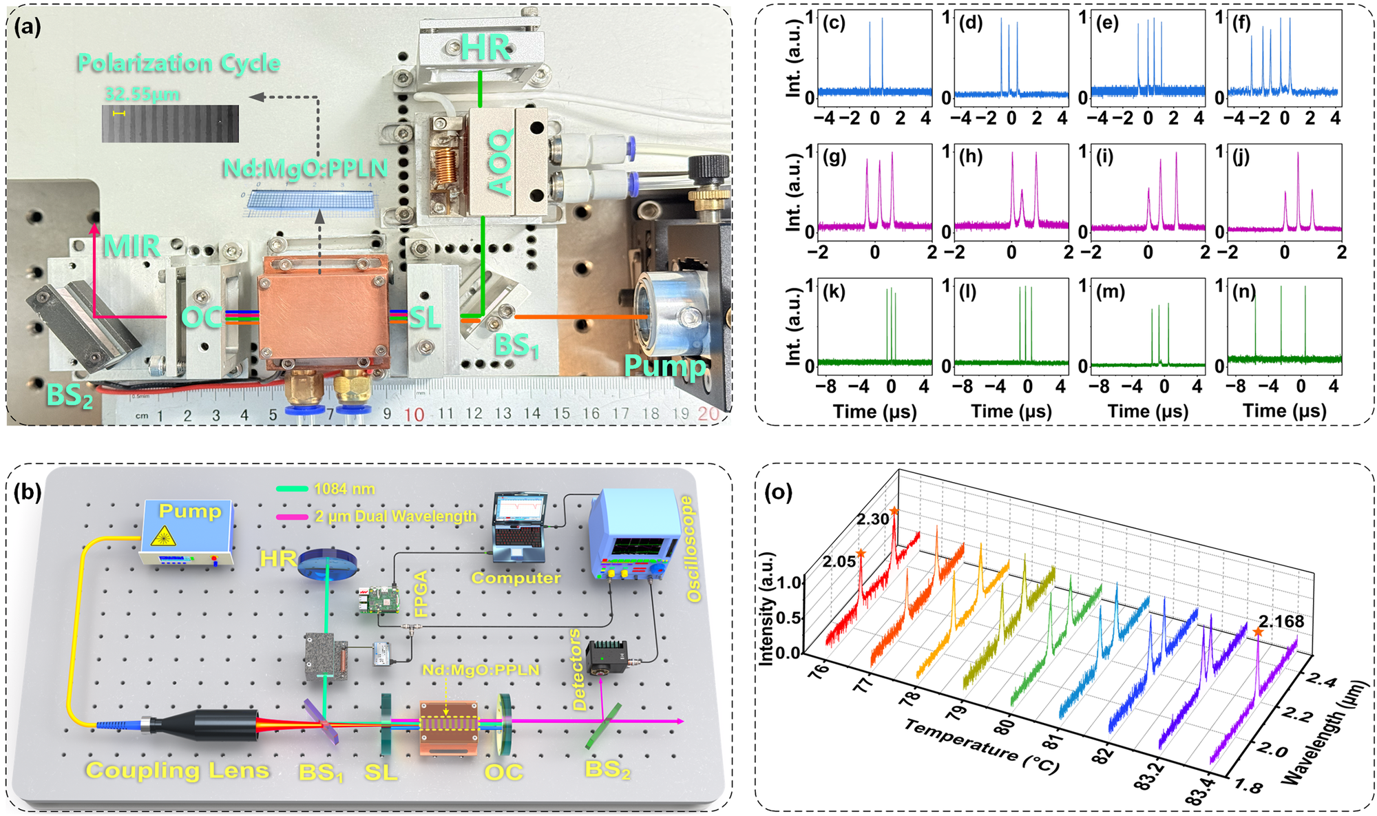
Figure 2 shows the experimental setup and representative results of the tunable dual-wavelength, encodable pulse-burst self-OPO. Figure 2(a) shows a photograph of the experimental setup, while Figure 2(b) shows a schematic diagram of the experimental setup. The 888 nm pump beam was delivered through a fiber with a core diameter of 400 μm and coupled into the Nd:MgO:PPLN crystal by a 1:1.5 coupling lens system. A single Nd:MgO:PPLN crystal provides both laser gain and nonlinear frequency conversion. The crystal used in the experiment had a Nd3+ doping concentration of 0.4% (atomic fraction), a poling period of 32.55 μm and dimensions of 6 mm × 2 mm × 40 mm.
Experimental setup and representative results of the tunable dual-wavelength, encodable pulse-burst self-OPO. (a) Photograph of the experimental setup. (b) Schematic of the experimental setup. (c)–(n) Measured programmable pulse-burst waveforms under different step-loss conditions, showing programmable control of the sub-pulse number, spacing and amplitude. (o) Dual-wavelength output spectra measured at different crystal temperatures, showing the continuous wavelength tuning from 2.05/2.30 μm at 76°C to the degenerate output at 2.168 μm at 83.4°C.

Figure 2 Long description
The image consists of fifteen panels labeled a through o.
Panel a is a top-down photo of an optical breadboard. A green laser path originates from a Pump, passes through a beam splitter B S sub 1, an A O Q modulator, and reflects off an H R mirror. It enters a copper-housed N d M g O P P L N crystal. A pink M I R beam exits through an O C and reflects off B S sub 2. Insets show a Polarization Cycle of 32.55 micrometers.
Panel b is a 3 D schematic of the same setup. It adds peripheral electronics including an F P G A, a Computer, and an Oscilloscope connected to Detectors. The optical path is color-coded with 1084 nanometers in green and 2 micrometer Dual Wavelength in pink.
Panels c through n are twelve line graphs of Intensity in arbitrary units versus Time in microseconds. They are organized in three rows of four. The top row (blue) shows increasing sub-pulse numbers from two to five. The middle row (purple) shows varying pulse spacing. The bottom row (green) shows varying pulse amplitudes.
Panel o is a 3 D waterfall plot. The x-axis is Temperature in degrees Celsius from 76 to 83.4. The y-axis is Intensity in arbitrary units. The z-axis is Wavelength in micrometers from 1.8 to 2.4. At 76 degrees, two distinct peaks appear at 2.05 and 2.30 micrometers. As temperature increases, the peaks converge until they merge into a single degenerate output at 2.168 micrometers at 83.4 degrees Celsius.
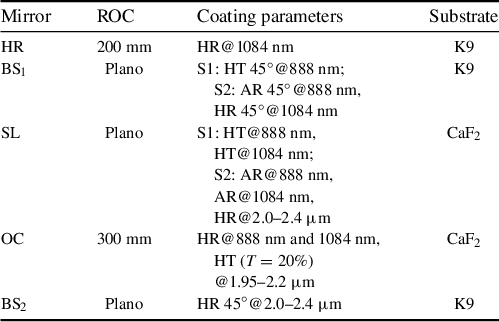
The laser employed an L-shaped composite resonator. The 1084 nm fundamental cavity was formed by a high-reflectivity (HR) mirror, a 45° beam splitter (BS1) and an output coupler (OC), whereas the OPO cavity was formed by an OPO HR mirror (SL) and the same OC. In this configuration, the fundamental oscillation and optical parametric oscillation share the Nd:MgO:PPLN crystal and part of the cavity mirrors, allowing the fundamental laser field and the 2 μm parametric waves to be generated cooperatively in a compact self-OPO cavity. The detailed coating specifications of the cavity mirrors are provided in Table 1.
Detailed specifications of the cavity mirrors used in the tunable dual-wavelength, encodable pulse-burst self-OPO a .

Table 1 Long description
The table consists of four columns: Mirror, R O C (radius of curvature), Coating parameters, and Substrate.
* Row 1: Mirror H R. R O C is 200 mm. Coating is H R at 1084 nm. Substrate is K 9.
* Row 2: Mirror B S sub 1. R O C is Plano. Coating S 1 is H T 45 degrees at 888 nm. Coating S 2 is A R 45 degrees at 888 nm and H R 45 degrees at 1084 nm. Substrate is K 9.
* Row 3: Mirror S L. R O C is Plano. Coating S 1 is H T at 888 nm and H T at 1084 nm. Coating S 2 is A R at 888 nm, A R at 1084 nm, and H R at 2.0 to 2.4 micrometers. Substrate is C a F sub 2.
* Row 4: Mirror O C. R O C is 300 mm. Coating is H R at 888 nm and 1084 nm, and H T (T equals 20 percent) at 1.95 to 2.2 micrometers. Substrate is C a F sub 2.
* Row 5: Mirror B S sub 2. R O C is Plano. Coating is H R 45 degrees at 2.0 to 2.4 micrometers. Substrate is K 9.
a ROC, radius of curvature; HT, high transmissivity; HR, high reflectivity; AR, antireflection; HR 45°, 45° high reflectivity.
An acousto-optic Q-switch was inserted into the 1084 nm fundamental cavity to modulate the intracavity loss. A stepwise signal, S Q(t), was generated by an FPGA under computer control and applied to the acousto-optic Q-switch driver. The corresponding acoustic field introduced controllable diffraction loss into the fundamental cavity, resulting in stepwise modulation of the cavity Q factor. By programming the step number, step interval and step amplitude, the population inversion accumulated within each Q-switching cycle could be released in a staged manner, thereby regulating the sub-pulse number, temporal spacing and amplitude. Because the temporal modulation of the fundamental field is transferred to the 2 μm parametric output through nonlinear frequency conversion, programmable pulse-burst encoding can be achieved at the 2 μm output. The corresponding numerical simulations of the inversion-density evolution and encoded pulse-burst formation are provided in Section S1 in the Supplementary Material.
In addition to temporal modulation, the dual-wavelength output was controlled by temperature tuning of the quasi-phase-matching condition. As the crystal temperature increased, the signal and idler wavelengths shifted toward the near-degenerate regime. The theoretical calculation predicts signal–idler degeneracy at 2.168 μm at a crystal temperature of 83.4°C. Experimentally, when the crystal temperature was increased from 76°C to 83.4°C, the dual-wavelength output evolved from 2.05/2.30 μm at 76°C to a degenerate output at 2.168 μm at 83.4°C. The detailed calculation procedure is provided in Section S2 in the Supplementary Material.
The average output power was measured with a power meter (Ophir F150A-BB-26-V1), and the temporal waveforms were recorded using a digital oscilloscope (Yokogawa DLM3024) together with a pulse detector (Vigo PCI-3TE-12). The energy of a single pulse envelope was calculated from the average output power and the pulse-envelope repetition rate. Combined with the time-domain waveforms recorded by the oscilloscope, the ratio of the integrated area of each sub-pulse to the total integrated area was used as the energy distribution coefficient, from which the energy of each sub-pulse was obtained. The output spectra and radio-frequency (RF) spectra were measured using an optical spectrum analyzer (Yokogawa AQ6375) and an RF spectrum analyzer (Keysight Technologies N9000B), respectively. The beam radius and spatial beam profile of the output laser were characterized with a beam profiling camera (Ophir PY-IV-C-A-PRO).
3 Results and discussion
3.1 Effects of step voltages V2 and V3 on sub-pulse characteristics
To describe the stepwise modulation of intracavity loss induced by acousto-optic Q-switching, the time-dependent loss within a single Q-switching cycle is denoted as β(t), and the corresponding Q-switching signal is denoted as S Q(t). Here, n is the number of steps, βi is the intracavity loss corresponding to the ith step, Δti is the duration of the ith step, ti is the falling time of the ith step and Vi is the acousto-optic driving voltage corresponding to that loss level. By programming n, Δti and Vi , the evolution of intracavity loss can be flexibly controlled, thereby enabling programmable control of the sub-pulse number, temporal spacing and amplitude distribution within the pulse burst, as well as encodable pulse-burst output.
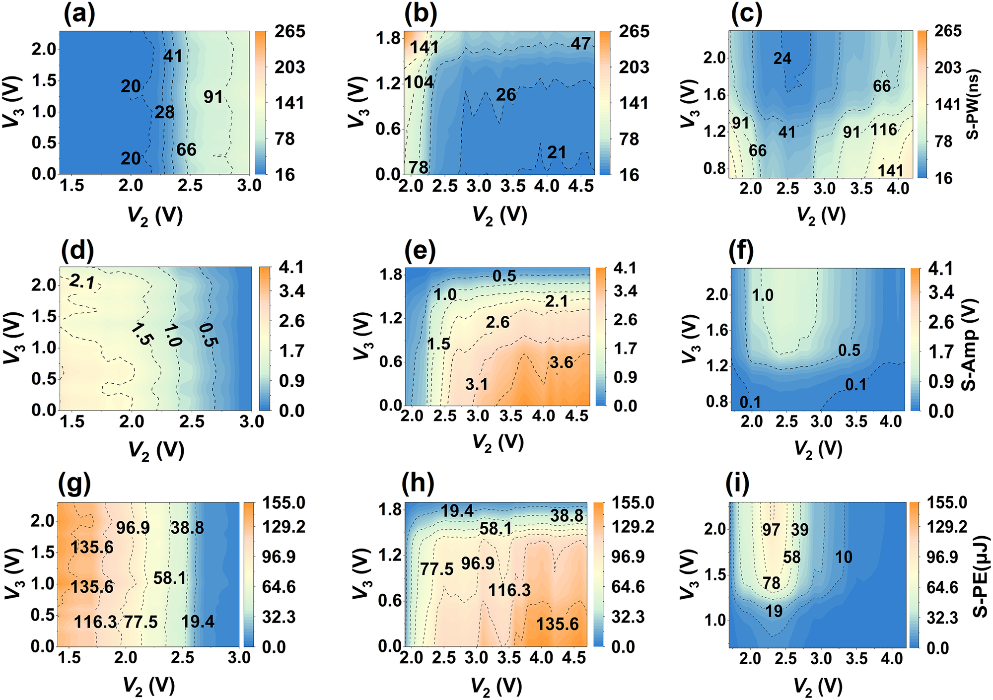
Under the conditions of a step number of n = 3, a Q-switching repetition frequency of f Q = 10 kHz, a pump power of 27 W and fixed step intervals of Δt 2 = Δt 3 = 700 ns, we experimentally investigated the effects of the step voltages V 2 and V 3 on the pulse width, amplitude and energy of the first, second and third sub-pulses within each pulse burst. Based on the measured results, filled contour maps of the sub-pulse width, amplitude and energy were plotted in the (V 2, V 3) parameter plane, as shown in Figure 3. The horizontal axis represents V 2, the vertical axis represents V 3 and the color scale indicates the corresponding sub-pulse width, amplitude or energy. For the first sub-pulse, V 2 and V 3 were varied over 1.4–3 and 0–2.3 V, respectively; for the second sub-pulse, over 1.9–4.7 and 0–1.9 V, respectively; and for the third sub-pulse, over 1.7–4.2 and 0.7–2.3 V, respectively.
Two-dimensional contour maps of sub-pulse characteristics in the (V 2, V 3) plane. (a)–(c) Sub-pulse width (S-PW i ), (d)–(f) sub-pulse amplitude (S-Amp i ) and (g)–(i) sub-pulse energy (S-PE i ), where i = 1, 2, 3 denotes the sub-pulse index. In each group, the panels from left to right correspond to the first, second and third sub-pulses, respectively. The color scales represent sub-pulse width (ns), sub-pulse amplitude (V) and sub-pulse energy (μJ), respectively.

Figure 3 Long description
A grid of nine two-dimensional contour maps organized into three rows.
Row 1 (panels a, b, c) displays S-P W sub i (sub-pulse width in nanoseconds). The X-axis is V sub 2 (V) and the Y-axis is V sub 3 (V). The color scale ranges from blue (16) to orange (265). Panel (a) shows width increasing from left to right. Panel (b) shows a sharp increase at low V sub 2. Panel (c) shows a complex central valley of lower width values.
Row 2 (panels d, e, f) displays S-Amp sub i (sub-pulse amplitude in Volts). The axes remain V sub 2 and V sub 3. The color scale ranges from blue (0.0) to orange (4.1). Panel (d) shows amplitude decreasing as V sub 2 increases. Panel (e) shows amplitude increasing toward the bottom-right corner. Panel (f) shows a central region of higher amplitude surrounded by lower values.
Row 3 (panels g, h, i) displays S-P E sub i (sub-pulse energy in micro-Joules). The axes remain V sub 2 and V sub 3. The color scale ranges from blue (0.0) to orange (155.0). Panel (g) shows energy decreasing from left to right. Panel (h) shows energy increasing toward the bottom-right. Panel (i) shows a localized peak of energy in the center-left region.
Across all panels, dashed contour lines delineate specific value thresholds, with numerical labels such as 20, 66, 91 for width; 0.5, 1.5, 3.1 for amplitude; and 19.4, 77.5, 135.6 for energy.
Figures 3(a)–3(c) depict the widths of the three sub-pulses, denoted as S-PW i (i = 1, 2, 3), across the (V 2, V 3) plane. S-PW1 is dominated by V 2, remaining low (~18–35 ns) for V 2 ≤ 2.1 V, undergoing a threshold-like transition at V 2 ≈ 2.2–2.4 V and subsequently reaching a high-width plateau (≥80 ns), with a minimum of 15.99 ns at (V 2, V 3) = (1.5, 2.0) V. S-PW2 exhibits an approximately diagonal gradient, decreasing with V 2 and increasing with V 3, with the smallest values in the high-V 2/low-V 3 region; the minimum reaches 19.29 ns at (4.1, 0) V. S-PW3 shows a U-shaped dependence on V 2 and generally decreases with V 3, reaching its minimum (21.74 ns) near moderate V 2 and higher V 3 (2.5, 2.2) V. Overall, V 2 mainly governs S-PW1, narrow S-PW2 requires high V 2 and low V 3 and minimum S-PW3 occurs at moderate V 2 with higher V 3, providing guidance for sub-pulse shaping and robust operating-window selection. The reproducibility of the sub-pulse widths was further examined under a modulation condition with a step interval of 1 μs, and the corresponding results are provided in Section S3 in the Supplementary Material.
Figures 3(d)–3(f) present the two-dimensional contour maps of the three sub-pulse amplitudes, S-Amp i (i = 1, 2, 3), in the (V 2, V 3) plane. S-Amp1 decreases significantly with increasing V 2, exhibiting a high-amplitude band at V 2 < 2.1 V and a low-amplitude region at V 2 > 2.7 V, with only weak dependence on V 3. S-Amp2 depends strongly on both V 2 and V 3, increasing with V 2 and decreasing with V 3, which reflects the role of the second step-loss jump in determining the second sub-pulse amplitude. By comparison, S-Amp3 is more sensitive to V 3, while V 2 mainly provides fine tuning. A relatively high S-Amp3 appears at intermediate V 2 and large V 3, whereas low amplitudes are obtained at small V 3 or at the two ends of the V 2 range. These results show that V 2 and V 3 provide distinct but complementary control over the amplitude distribution of the three sub-pulses.
Figures 3(g)–3(i) show the two-dimensional contour maps of the sub-pulse energies, S-PE i (i = 1, 2, 3), in the (V 2, V 3) plane. S-PE1 is mainly governed by V 2, gradually decreasing as V 2 increases, while showing only weak dependence on V 3. Specifically, the energy remains of the order of 100 μJ at V 2 ≈ 1.5 V, but decreases to below 40 μJ when V 2 increases to about 2.5–3.0 V. In contrast, S-PE2 is strongly influenced by both V 2 and V 3. It generally increases with V 2, especially at low V 3, rising from a few tens of microjoules to about 110–140 μJ before approaching saturation, while increasing V 3 suppresses the second-sub-pulse energy. For S-PE3, the energy distribution is more localized. In most of the (V 2, V 3) plane, S-PE3 remains low, and a pronounced increase appears only in a limited region around V 2 ≈ 2.2 V and V 3 > 1.5 V, where it reaches about 70–90 μJ. Overall, the first sub-pulse energy is mainly controlled by V 2, the second depends on both V 2 and V 3 and appreciable energy in the third sub-pulse appears only within a confined parameter region. These trends provide useful guidance for programmable energy shaping and encoding-state selection.
It should be noted that the sub-pulse number, intra-burst spacing and amplitude distribution are interdependent. Under fixed pump power and fixed Q-switch repetition frequency, the sub-pulse number is mainly determined by the number of Q-switch voltage steps, whereas the intra-burst spacing is controlled by the time interval between adjacent steps. The amplitude distribution is mainly adjusted by the step voltage levels, but it is also affected by the intra-burst spacing through the gain depletion and recovery processes.
For the three-sub-pulse equal-amplitude operation, when Δt 1 and Δt 3 are kept unchanged and only Δt 2 is varied in the nanosecond to sub-microsecond range, the first sub-pulse amplitude remains approximately unchanged. Increasing Δt 2 provides a longer gain recovery time before the second sub-pulse, so the second sub-pulse amplitude tends to increase. The enhanced second sub-pulse then extracts more gain, causing the third sub-pulse amplitude to decrease. Conversely, decreasing Δt 2 tends to reduce the second sub-pulse amplitude and increase the third sub-pulse amplitude.
As an empirical tuning guideline, the sub-pulse number and spacing can be selected first, and the previously optimized voltage set can then be used as the initial condition. Only the relevant step voltage needs to be fine-tuned to recover the desired amplitude distribution. In our experiment, increasing V 3 helps suppress the second sub-pulse and enhance the third sub-pulse, while decreasing V 3 produces the opposite adjustment.
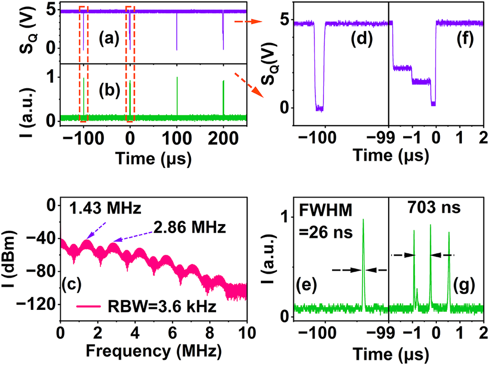
Time-domain waveforms and RF spectrum of the alternating ‘1-3-1-3’ pulse-burst sequence. (a) Alternating single-step and three-step Q-switch modulation signal, S Q(t). (b) Pulse-burst output with alternating sub-pulse numbers in a ‘1-3-1-3’ sequence. (c) RF spectrum of the ‘1-3-1-3’ sequence. (d), (e) Zoomed-in views of the Q-switch signal and the corresponding output waveform in the single-pulse envelope. (f), (g) Zoomed-in views of the Q-switch signal and the corresponding output waveform in the three-pulse envelope.

Figure 4 Long description
The multi-panel figure is organized as follows.
* Top-left panels (a) and (b): Two stacked line graphs sharing a horizontal axis of Time in microseconds from minus 150 to 250. Panel (a) shows the Q-switch signal S Q in Volts as a purple line with downward spikes. Panel (b) shows the output intensity I in arbitrary units as a green line with upward pulses corresponding to the spikes in (a).
* Top-right panels (d) and (f): Zoomed-in views of the purple S Q signal. Panel (d) shows a single-step rectangular dip at minus 100 microseconds. Panel (f) shows a three-step staircase-like dip between minus 1 and 0 microseconds.
* Bottom-left panel (c): A line graph of R F spectrum showing Intensity I in d B m versus Frequency in M H z from 0 to 10. The pink trace shows periodic lobes with peaks labeled at 1.43 M H z and 2.86 M H z. The R B W is 3.6 k H z.
* Bottom-right panels (e) and (g): Zoomed-in views of the green output intensity I. Panel (e) shows a single narrow pulse at minus 99.5 microseconds with a F W H M of 26 nanoseconds. Panel (g) shows a burst of three pulses between minus 1 and 1 microsecond with a total burst duration labeled as 703 nanoseconds.
3.2 Alternating sub-pulse numbers
To obtain alternating sub-pulse numbers, we program two Q-switch step waveforms (n = 1 and n = 3) and alternate them over a super period, generating a pulse burst with alternating sub-pulse numbers. Figure 4 shows the temporal and spectral characteristics of a ‘1-3-1-3’ alternating pulse burst. As shown in Figures 4(a) and 4(b), the Q-switch modulation signal and the corresponding laser output exhibit an alternating 1-3-1-3 pulse-burst pattern. The Q-switch repetition frequency was 10 kHz, corresponding to a 100 μs interval between adjacent pulse-burst envelopes. In this alternating pattern, one complete ‘1-3’ coding cycle consists of two adjacent envelopes, namely one single-pulse envelope and one three-pulse envelope. Therefore, the ‘1-3’ coding-cycle period is 200 μs, corresponding to a coding-cycle frequency of 5 kHz. Figures 4(d) and 4(e) zoom in on the first type of envelope, where a single opening of the Q-switch produces a single pulse with a full width at half maximum (FWHM) of about 26 ns. Figures 4(f) and 4(g) zoom in on the second type of envelope, in which the multi-step drive waveform generates three sub-pulses within a 100 μs period. These sub-pulses have nearly identical amplitudes, and the measured adjacent sub-pulse spacing is approximately 703 ns, confirming that the intra-burst timing is precisely defined by the preset step duration of the acousto-optic loss modulation. The RF spectrum in Figure 4(c), measured with a resolution bandwidth of 3.6 kHz, shows a clear interference envelope with pronounced peaks near 1.43 and 2.86 MHz. Complementary frequency-domain characterization of the low-frequency envelope repetition structure is provided in Figure S6 in the Supplementary Material. These frequencies correspond to 1/Δt 1 and are consistent with the Fourier transform of a three-pulse burst, indicating that the RF spectrum consists of combs with 5 kHz spacing whose amplitudes are modulated by the temporal interference envelope of the three sub-pulses. The gradual roll-off at higher frequencies is determined by the finite 26 ns width of each sub-pulse. The good agreement between the time-domain waveform and the RF spectrum further confirms that the FPGA-controlled stepwise Q-switching can deterministically generate alternating pulse-burst patterns with a programmable sub-pulse number.
3.3 Alternating sub-pulse spacing
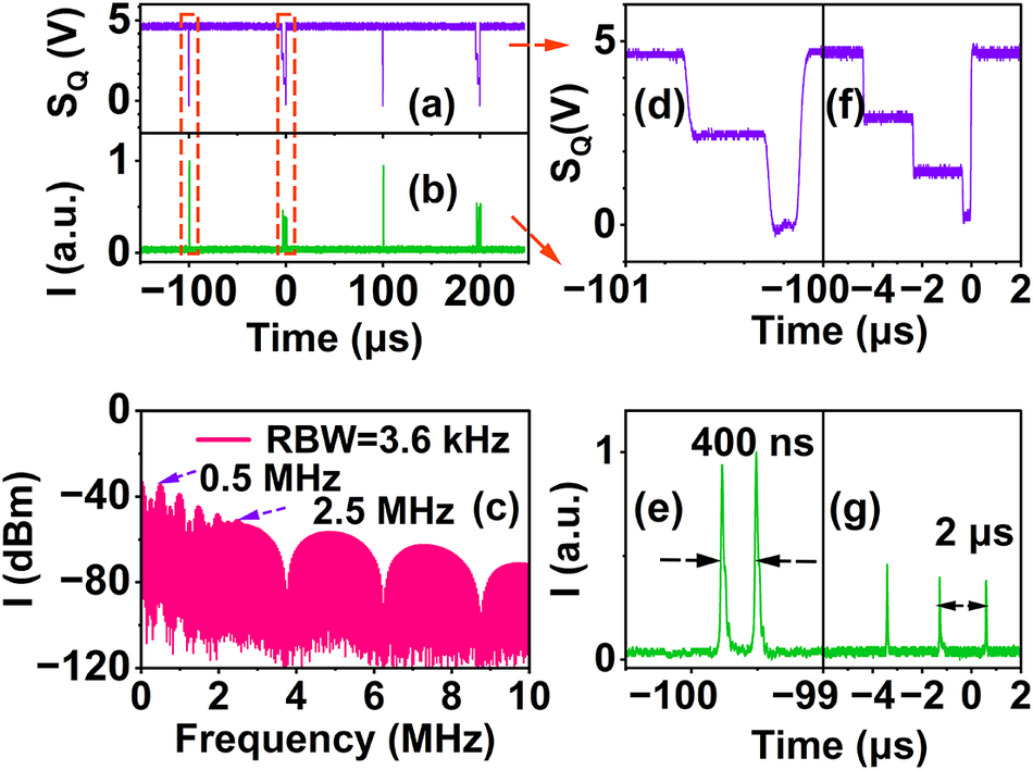
Figure 5 shows that stepwise acousto-optic Q-switching enables alternating pulse bursts with hybrid nanosecond–microsecond sub-pulse spacings. The measured modulation S Q(t) (Figure 5(a)) alternates between a two-step pattern (n = 3, Δt 2 = 400 ns) and a three-step pattern (n = 4, Δt 2 = Δt 3 = 2 μs), both with a 100 μs period, yielding a 10 kHz envelope repetition rate and a 200 μs super period. Accordingly, the waveform (Figure 5(b)) alternates between a two-sub-pulse envelope with 400 ns spacing (Figures 5(d) and 5(e)) and a three-sub-pulse envelope with approximately 2 μs spacing (Figures 5(f) and 5(g)), confirming deterministic, FPGA-programmable control of sub-pulse spacing from hundreds of nanoseconds to microseconds. The measured RF spectrum (Figure 5(c), resolution bandwidth (RBW) 3.6 kHz) exhibits pronounced peaks near 2.5 and 0.5 MHz, consistent with the inverse spacings 1/Δt 2 = 1/400 ns = 2.5 MHz and 1/Δt 3 = 1/2 μs = 0.5 MHz, respectively. The spectrum can be interpreted as a 5 kHz comb (set by the 200 μs super period) whose line amplitudes are shaped by the interference envelopes of the two- and three-pulse structures, in good agreement with the time-domain waveforms.
Time-domain waveforms and RF spectrum of the alternating ‘nanosecond–microsecond’ pulse-burst sequence. (a) Q-switch modulation signal with alternating nanosecond- and microsecond-spaced patterns. (b) Corresponding pulse-burst waveform with alternating nanosecond–microsecond spacings. (c) RF spectrum of the alternating nanosecond–microsecond sequence. (d), (e) Zoomed-in views of the Q-switch signal and the corresponding output waveform for the nanosecond-spaced envelope. (f), (g) Zoomed-in views of the Q-switch signal and the corresponding output waveform for the microsecond-spaced envelope.

Figure 5 Long description
A multi-panel set of line graphs.
Panel a and b: Two stacked time-domain graphs sharing an x-axis from minus 150 to 250 microseconds. Panel a shows the Q-switch signal S sub Q in Volts, featuring a purple baseline at 5 Volts with downward spikes. Panel b shows the intensity I in arbitrary units, featuring a green baseline at 0 with upward pulse bursts corresponding to the spikes in a. Red dashed boxes highlight regions at minus 100 and 0 microseconds.
Panel d and f: Zoomed-in views of the purple Q-switch signal. Panel d shows a single step-down pulse around minus 100 microseconds. Panel f shows a multi-step staircase-like pulse sequence between minus 4 and 0 microseconds.
Panel c: R F spectrum showing intensity I in d B m versus frequency from 0 to 10 M H z. The pink data shows a series of lobes with peaks labeled at 0.5 M H z and 2.5 M H z. The resolution bandwidth R B W is 3.6 k H z.
Panel e and g: Zoomed-in views of the green pulse intensity. Panel e shows two sharp pulses separated by 400 n s near the minus 100 microsecond mark. Panel g shows a sequence of pulses separated by 2 microseconds between the minus 4 and 0 microsecond marks.
3.4 Alternating sub-pulse amplitude
Figure 6 further demonstrates the pulse bursts with alternating amplitudes. In Figure 6(a), the FPGA-generated Q-switch modulation signal S Q(t) alternates between two modes within a 300 μs super period. The first mode applies a three-step waveform, in which the voltage-drop amplitude at the second step is greatly reduced, so the corresponding Q-switch opening is much weaker than at the first and third steps. The second mode applies a two-step waveform, where the two Q-switch openings have nearly the same strength. As a result, the output in Figure 6(b) forms an alternating ‘high–low–high/high–high’ pulse sequence: the first envelope effectively contains two sub-pulses separated by 2 μs, with the middle pulse strongly suppressed, while the second envelope contains two high-amplitude sub-pulses separated by 1 μs. The entire pattern repeats with a 300 μs super period, and the time interval between the first sub-pulses of two adjacent envelopes is 100 μs. Figures 6(d) and 6(e) show magnified views of the control signal and output waveform for the first envelope type. The three-step drive yields two dominant pulses separated by 2 μs, while the central sub-pulse (normalized amplitude ≈ 0.2) acts as a weak marker between two high-energy pulses (>0.76). Figures 6(f) and 6(g) show a second envelope type, in which a two-step control signal opens the cavity twice with comparable loss, generating two nearly identical sub-pulses separated by 1 μs. These time-domain results show that stepwise Q-switching enables programmable control of sub-pulse spacing together with deterministic tuning of the relative amplitudes and energies of the sub-pulses within each burst. The RF spectrum of the amplitude-alternating sequence, measured with a resolution bandwidth of 2 kHz, is presented in Figure 6(c). Distinct peaks appear near 0.5 and 1 MHz, in good agreement with the inverse spacings of the two pulse envelopes. Accordingly, the alternating envelopes impose two interference patterns on a single RF comb, producing a composite spectral envelope with maxima at 0.5 and 1 MHz and minima at the corresponding fractional frequencies. The agreement between the measured RF spectrum and the programmed temporal structure confirms the flexible synthesis of amplitude-alternating pulse bursts and highlights an additional degree of freedom for burst-level encoding and modulation. Complementary low-frequency RF characterization of the amplitude-alternating sequence is provided in Figure S7 in the Supplementary Material.
Pulse-burst sequence with alternating sub-pulse amplitudes. (a) Q-switch modulation signal for the ‘high–low–high/high–high’ amplitude-alternating pulse-burst sequence. (b) Corresponding pulse-burst waveform showing the alternating ‘high–low–high/high–high’ sequence. (c) RF spectrum of the amplitude-alternating sequence. (d), (e) Enlarged views of the control signal and the corresponding output waveform for the first envelope type. (f), (g) Enlarged views of the control signal and the corresponding output waveform for the second envelope type.

Figure 6 Long description
The multi-panel figure is organized as follows:
* Top-Left (Panels a and b): Two stacked line graphs sharing a Time axis in microseconds from -400 to 400. Panel a shows a purple signal S sub Q in Volts, maintaining a baseline of 5 Volts with periodic downward spikes. Panel b shows a green intensity signal I in arbitrary units with corresponding upward pulses. Red dashed boxes highlight two specific pulse groups.
* Bottom-Left (Panel c): A line graph of an R F spectrum. The x-axis is Frequency in M H z from 0 to 5. The y-axis is Intensity I in d B m from -120 to 0. The signal shows a series of lobes with peaks at 0.5 M H z and 1 M H z. A legend indicates R B W equals 3.6 k H z.
* Top-Right (Panels d and f): Enlarged views of the purple S sub Q signal. Panel d shows a stepped downward modulation between -4 and 2 microseconds. Panel f shows a similar stepped modulation between 96 and 104 microseconds.
* Bottom-Right (Panels e and g): Enlarged views of the green intensity signal. Panel e shows three pulses of varying heights (labeled 0.2 and 0.76) with a 2 microsecond interval. Panel g shows two closely spaced pulses with a 1 microsecond interval.
In the RF spectra, the main peaks correspond to the designed temporal modulation features of the pulse bursts. Besides these main components, weak sideband-like components and spectral ripples can also be observed. These features mainly arise from the finite pulse-burst structure and the residual loss modulation introduced by the stepwise Q-switching process. Since the pulse bursts consist of a finite number of sub-pulses rather than an infinite ideal pulse train, the corresponding Fourier spectra can exhibit a sinc-like spectral envelope and sidelobe structures. The finite response of the RF-driven acousto-optic modulator (AOM), nonideal RF switching edges and residual intracavity loss modulation may further introduce additional spectral components. Pulse-to-pulse amplitude fluctuations can also increase the noise floor. Since the RF peaks remain clearly resolved without obvious broadening and the corresponding time-domain pulse structures are stable, timing jitter is not considered the dominant contribution.
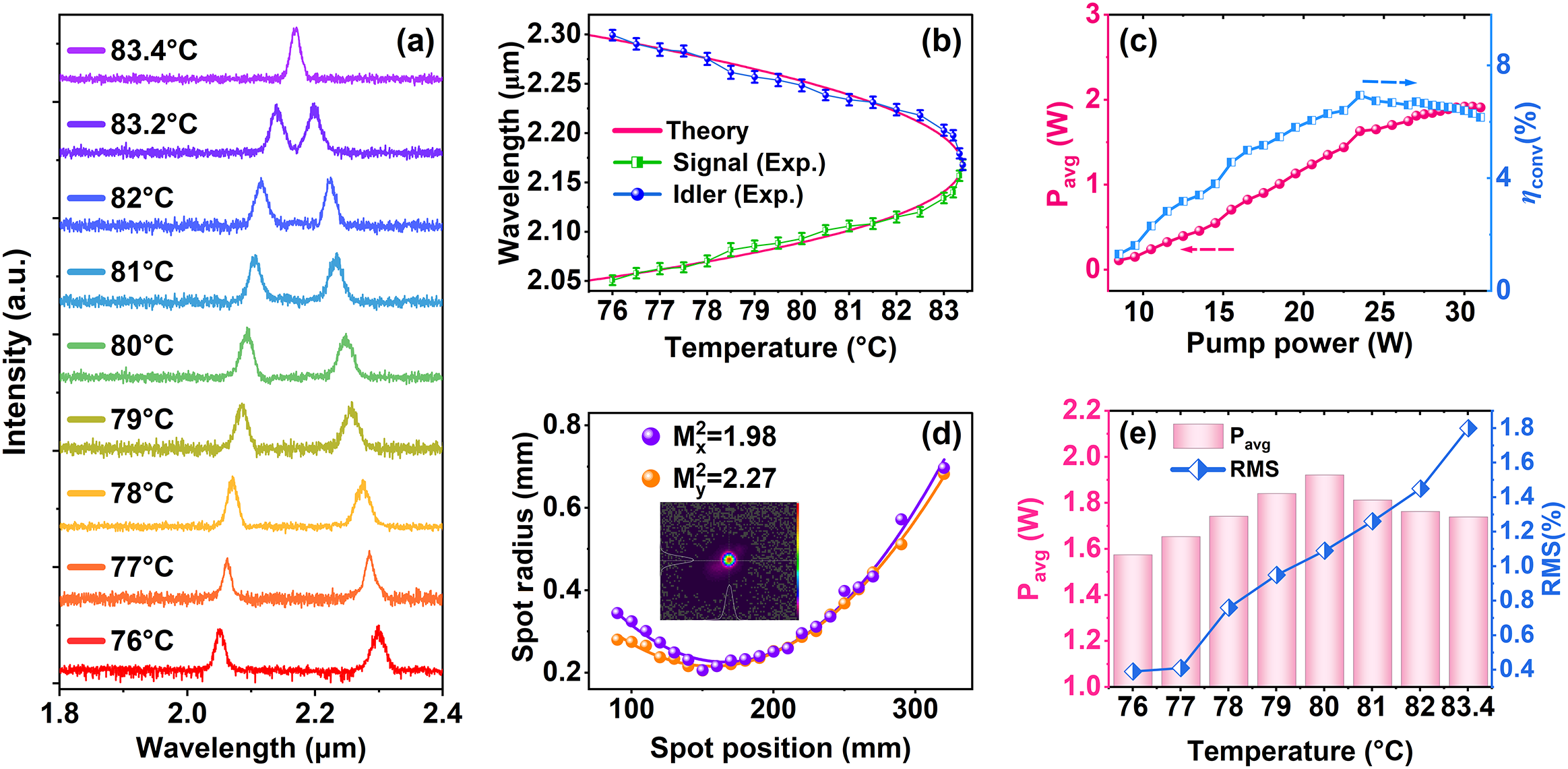
Output characteristics of the tunable-spacing dual-wavelength programmable pulse burst under the alternating ‘1-3-1-3’ sub-pulse-number regime. (a) Dual-wavelength spectra measured at different crystal temperatures, showing temperature-tunable wavelength spacing. (b) Comparison between experimental and theoretical QPM wavelengths. (c) Average output power and optical-to-optical conversion efficiency versus pump power at 80°C. (d) Beam quality measurement of the output laser. (e) Average output power and RMS power fluctuation of the combined dual-wavelength output at different crystal temperatures.

Figure 7 Long description
A multi-panel figure with five charts labeled (a) through (e).
Panel (a) is a stacked line graph of Intensity in arbitrary units versus Wavelength in micrometers from 1.8 to 2.4. It shows spectral peaks for temperatures from 76 to 83.4 degrees Celsius. As temperature increases, the two distinct peaks move closer together until they merge into a single peak at 83.4 degrees Celsius.
Panel (b) is a line graph of Wavelength in micrometers versus Temperature in degrees Celsius. A pink theoretical curve forms a sideways parabola. Experimental data for Signal and Idler wavelengths, marked with green squares and blue circles with error bars, follow the theoretical curve, converging at approximately 2.16 micrometers at 83.4 degrees Celsius.
Panel (c) is a dual-axis line graph. The left Y-axis is P sub avg in Watts (0 to 3) and the right Y-axis is optical-to-optical conversion efficiency eta sub conv in percent (0 to 8). Both average power (pink circles) and efficiency (blue squares) show a linear increase with pump power from 10 to 24 Watts, followed by a plateau.
Panel (d) is a line graph of Spot radius in millimeters versus Spot position in millimeters. Two parabolic curves for M super 2 sub x equals 1.98 (purple) and M super 2 sub y equals 2.27 (orange) show a minimum radius near 150 millimeters. An inset shows a circular laser beam profile.
Panel (e) is a dual-axis chart. The left Y-axis is P sub avg in Watts (1.0 to 2.2) shown as pink bars. The right Y-axis is R M S percentage (0.4 to 1.8) shown as a blue line with diamonds. As temperature increases from 76 to 83.4 degrees Celsius, the average power peaks at 80 degrees Celsius while the R M S power fluctuation increases steadily.
Under the alternating ‘1-3-1-3’ sub-pulse-number regime, the output characteristics of the tunable dual-wavelength programmable pulse burst are systematically characterized, as shown in Figure 7. By varying the temperature of the Nd:MgO:PPLN crystal, the quasi-phase-matching condition is modified, enabling tunable control of both the dual-wavelength output and its wavelength spacing. As shown in Figure 7(a), the temperature-dependent output spectra were recorded at crystal temperatures of 76°C, 77°C, 78°C, 79°C, 80°C, 81°C, 82°C, 83.2°C and 83.4°C. At 76°C, the dual-wavelength output was located at 2.05 and 2.30 μm. With increasing temperature, the short-wavelength component gradually shifted toward longer wavelengths, whereas the long-wavelength component shifted toward shorter wavelengths, indicating that the two wavelength branches continuously approached the degeneracy point. When the temperature was increased to 83.4°C, the two branches merged into a degenerate output at 2.168 μm. The measured tuning trend is in good agreement with the theoretical quasi-phase-matching (QPM) calculation. Figure 7(b) compares the experimental wavelength data with the theoretical QPM wavelength curves. The experimental data represent the average values of five repeated measurements at each temperature, with the standard deviations shown as error bars. The experimental results agree well with the theoretical curves, confirming the QPM-based temperature-tuning behavior of the dual-wavelength output. Figure 7(c) shows the output power and optical-to-optical conversion efficiency as functions of pump power at 80°C. At a pump power of 30 W, the maximum average output power reaches 1.92 W, and the fitted slope efficiency is 10.6%. The highest optical-to-optical conversion efficiency reaches 6.94% at a pump power of 23.5 W. In addition, the beam quality of the output laser is measured using a PY-IV-C-A-PRO pyroelectric array camera (Ophir Optronics Solutions Ltd.) in combination with a focusing lens of f = 150 mm, yielding Mx 2 = 1.98 and My 2 = 2.27, as shown in Figure 7(d). Figure 7(e) shows the average output power and root mean square (RMS) power fluctuation of the combined dual-wavelength output measured at different crystal temperatures under a pump power of 30 W. The average output power gradually increased from 76°C to 80°C and then slightly decreased from 80°C to 83.4°C. At the temperature corresponding to the highest average output power, the RMS power fluctuation was measured to be 1.09%. Meanwhile, the RMS power fluctuation increased over the entire temperature range, indicating a gradual degradation of output power stability as the two wavelength branches approached the degeneracy point. This degradation is likely related to the reduced wavelength spacing and enhanced mode competition near the degeneracy point.
3.5 Programmable pulse-burst information encoding
Through programmable control of the number, spacing and amplitudes of the sub-pulses, and by alternating among different parameter sets, we implement pulse-burst encoding, enabling the bursts to carry information on demand. As an example, we demonstrate a frame structure composed of five pulse envelopes, each containing five sub-pulses. Assigning logical ‘1’ and ‘0’ to high and low amplitudes, respectively, yields a 5-bit binary code capable of representing all uppercase letters. Figure 8 shows four pulse-burst patterns implementing the optical binary encoding of ‘CUST’ (the acronym of Changchun University of Science and Technology), while Figure 9 shows five pulse-burst patterns encoding ‘LASER’. Each letter is encoded with 5 bits; the total duration is 300 μs for ‘CUST’ and 1000 μs for ‘LASER’. The symbol duration is 4 μs, corresponding to a symbol rate of 0.25 MHz. For further visualization, the corresponding multi-letter data stream is shown in Figure 10. This multi-letter demonstration confirms the feasibility of pulse-burst encoding on this platform and indicates its potential for higher-capacity optical data transmission and processing. A composite representation of the amplitude-only pulse-burst codewords corresponding to different alphabetic symbols is provided in Figure S8 in the Supplementary Material.
Amplitude-decision encoding demonstration of a dual-wavelength pulse-burst sequence (‘CUST’). (a) S Q(t) programmed for ‘CUST’. (b) Encoded dual-wavelength pulse-burst waveform corresponding to ‘CUST’. (c) Enlarged views of each symbol and the extracted 5-bit binary codewords (BC), together with the decoded letters (sym) obtained from the codeword mapping.

Figure 8 Long description
A multi-panel figure with three stacked sections labeled a, b, and c.
Panel a is a line graph showing S sub Q in Volts on the y-axis ranging from 0 to 5, against Time in micro-seconds on the x-axis. A purple signal remains constant at 5 Volts with four distinct downward-pointing stepped pulses occurring at 0, 100, 200, and 300 micro-seconds.
Panel b shows the Intensity I in arbitrary units on the y-axis against the same Time x-axis. A green baseline signal at 0 is interrupted by four pulse bursts enclosed in red dashed boxes labeled 1, 2, 3, and 4, corresponding to the timing in panel a. A red arrow points from panel b down to panel c.
Panel c is a detailed view of the four pulse bursts. Each burst is shown in an individual sub-plot with a refined time scale.
* Burst 1 spans from minus 4 to 1 micro-seconds, showing two green peaks. Below the plot, the B C row shows 0 0 0 1 1 and the sym row shows the letter C.
* Burst 2 spans from 96 to 101 micro-seconds, showing three green peaks. Below, the B C row shows 1 0 1 0 1 and the sym row shows the letter U.
* Burst 3 spans from 196 to 201 micro-seconds, showing three green peaks. Below, the B C row shows 1 0 0 1 1 and the sym row shows the letter S.
* Burst 4 spans from 296 to 301 micro-seconds, showing two green peaks. Below, the B C row shows 1 0 1 0 0 and the sym row shows the letter T.
Amplitude-decision encoding demonstration of the dual-wavelength pulse-burst sequence (‘LASER’). (a) S Q(t) programmed for ‘LASER’. (b) Corresponding encoded dual-wavelength pulse-burst waveform. (c) Enlarged views of each symbol and the extracted 5-bit binary codewords (BC), together with the decoded letters (sym) obtained from the codeword mapping.

Figure 9 Long description
Panel a shows a purple line graph of S sub Q in Volts against Time in microseconds. The signal remains at 5 Volts with five sharp downward spikes to 0 Volts at approximately 200, 400, 600, 800, and 1000 microseconds.
Panel b shows a green line graph of Intensity in arbitrary units against Time. It features five pulse bursts labeled 1 through 5 in red, corresponding to the spikes in panel a. Each burst is enclosed in a red dashed box.
Panel c provides enlarged views of these five bursts.
* Burst 1 at 197 to 202 microseconds shows two peaks, mapped to B C 0 1 1 0 0 and symbol L.
* Burst 2 at 397 to 402 microseconds shows one peak at the end, mapped to B C 0 0 0 0 1 and symbol A.
* Burst 3 at 597 to 602 microseconds shows three peaks, mapped to B C 1 0 0 1 1 and symbol S.
* Burst 4 at 798 to 803 microseconds shows two peaks, mapped to B C 0 0 1 0 1 and symbol E.
* Burst 5 at 998 to 1003 microseconds shows two peaks, mapped to B C 1 0 0 1 0 and symbol R.
Each sub-panel in c includes a B C row of 5-bit binary codewords and a sym row for the decoded letter.
Matrix representation of the 5-bit amplitude-decision binary codewords for (a) ‘CUST’ and (b) ‘LASER’.

Figure 10 Long description
The figure contains two panels, a and b, each featuring a grid where the y-axis is labeled Pulse group and the x-axis is labeled Sub-pulse number from 1 to 5. To the right of each grid is a column labeled Sym.
Panel a, representing C U S T, has 4 rows.
* Row 1: Binary sequence 0, 0, 0, 1, 1 corresponding to the symbol C.
* Row 2: Binary sequence 1, 0, 1, 0, 1 corresponding to the symbol U.
* Row 3: Binary sequence 1, 0, 0, 1, 1 corresponding to the symbol S.
* Row 4: Binary sequence 1, 0, 1, 0, 0 corresponding to the symbol T.
Panel b, representing L A S E R, has 5 rows.
* Row 1: Binary sequence 0, 1, 1, 0, 0 corresponding to the symbol L.
* Row 2: Binary sequence 0, 0, 0, 0, 1 corresponding to the symbol A.
* Row 3: Binary sequence 1, 0, 0, 1, 1 corresponding to the symbol S.
* Row 4: Binary sequence 0, 0, 1, 0, 1 corresponding to the symbol E.
* Row 5: Binary sequence 1, 0, 0, 1, 0 corresponding to the symbol R.
In both panels, the number 0 is contained in a blue square and the number 1 is contained in an orange square. Symbols in the Sym column are contained in green squares.
For amplitude-decision encoding, the stability of the sub-pulse amplitude is critical because the bit state is determined by the amplitude level. The pump power stability was measured at an operating pump power of 23.5 W over 1 h, and the RMS fluctuation was 0.073%, corresponding to a standard deviation of approximately 0.017 W. To directly evaluate the decision reliability, the amplitude stability of the encoded pulse burst with the code ‘101’ was measured under the same modulation parameters: f Q = 10 kHz, Δt 2 = Δt 3 = 1 μs, V 1 = 4.7 V, V 2 = V 3 = 1.52 V and V 4 = 0 V. The system was continuously triggered 50 times using a Yokogawa DLM3024 oscilloscope. The average amplitudes of the first ‘1’, second ‘0’ and third ‘1’ pulses were 95.52, 25.88 and 91.50 mV, respectively, with standard deviations of 3.87, 0.96 and 5.92 mV. The maximum ‘0’ amplitude was 27.8 mV, whereas the minimum ‘1’ amplitude was 81.3 mV, giving a minimum amplitude gap of 53.5 mV. With a decision threshold of 58.69 mV, the margins from the measured ‘0’ and ‘1’ amplitude ranges to the threshold were 30.89 and 22.61 mV, respectively. In addition, the 3σ criterion was also satisfied. Let A 0 and A 1 denote the mean amplitudes of the ‘0’ and ‘1’ states, respectively, and σ0 and σ1 denote their corresponding standard deviations. Under this definition, A 0 + 3σ 0 = 28.76 mV and A 1 − 3σ 1 = 73.74 mV. These results indicate that the ‘0’ and ‘1’ amplitude levels are well separated, and pump-power-related amplitude fluctuations are unlikely to cause bit errors under the present experimental conditions.
Beyond the reliability of amplitude-decision encoding, the scalability of the output power is another important factor for practical applications of the proposed dual-wavelength programmable pulse-burst source.
Further power scaling is feasible by increasing the pump brightness, improving pump-mode matching, optimizing the cavity mode size and output coupling and enhancing the thermal management of the Nd:MgO:PPLN crystal. Nevertheless, the achievable power is restricted by thermal lensing, thermal-induced QPM detuning, resonator mode distortion, coating absorption or damage, nonlinear conversion saturation and dual-wavelength mode competition. In particular, when the two wavelength branches approach the degeneracy point, stronger mode competition and thermal sensitivity may degrade the output stability. Therefore, future power scaling should be accompanied by improved heat dissipation, optimized cavity design, a larger effective mode area and more robust crystal/coating configurations.
4 Conclusion
In summary, we develop a 2 μm self-OPO featuring co-tunable dual-wavelength output and encodable pulse-burst emission. The system employs a single Nd:MgO:PPLN crystal to simultaneously provide laser gain and nonlinear frequency conversion within the same medium. By temperature tuning of the crystal, the quasi-phase-matching condition is adjusted, enabling tunable control of both the dual-wavelength output and its wavelength spacing. As the crystal temperature increases from 76°C to 83.4°C, the dual-wavelength output evolves from 2.05/2.30 μm to a degenerate output at 2.168 μm, confirming the temperature-dependent co-tuning behavior toward the degeneracy point.
Furthermore, FPGA-driven stepwise acousto-optic Q-switching enables dynamic and programmable modulation of the intracavity loss, allowing flexible control over the number, temporal spacing and amplitude (or energy) of the sub-pulses. Based on this approach, alternating outputs in sub-pulse number, spacing and amplitude are achieved, and the experimental results verify the stability and reconfigurability of the alternating pulse-burst sequences. In addition, encodable pulse-burst output is demonstrated, and amplitude-decision encoding of ‘CUST’ and ‘LASER’ is successfully realized, confirming the source-level information-loading capability of the system. Under the alternating ‘1-3-1-3’ sub-pulse-number regime, a maximum average output power of 1.92 W is obtained at a crystal temperature of 80°C and a pump power of 30 W, corresponding to a slope efficiency of 10.6%. The highest optical-to-optical conversion efficiency reaches 6.94% at a pump power of 23.5 W. At the maximum output power, the beam quality factors are Mx 2 = 1.98 and My 2 = 2.27, and the power stability over 1 h is 1.09% (RMS).
These results demonstrate the integration of co-tunable dual-wavelength output, programmable pulse-burst control and source-level encoding in the 2 μm spectral region, and lay a foundation for the application of reconfigurable pulse-burst lasers in selective molecular sensing, cross-interference suppression and optical information encoding.
Supplementary material
The supplementary material for this article can be found at http://doi.org/10.1017/hpl.2026.10177.
Acknowledgements
This work was supported by the National Natural Science Foundation of China (Grant Nos. 62275031 and U24A2045) and the Natural Science Foundation of Jilin Province (Grant No. 20260101014JJ).




 Open access

