1 Introduction
The flow of a viscous liquid film coating the interior of a vertical rigid tube has been studied in many settings both theoretically and experimentally, given the interest in numerous engineering and biological applications where such flows arise. These studies can be challenging due to the need for an accurate modelling of the dynamics of the free surface between the liquid film and the air comprising the core region. In a previous paper (Camassa, Ogrosky & Olander (Reference Camassa, Ogrosky and Olander2014), referred to hereafter as Part 1) the authors studied the gravity-driven downwards flow of a viscous liquid film where the air played the simple role of maintaining constant pressure at the interface. It was shown there that a model derived using long-wave asymptotics was able to quantitatively describe the flow of such films in experiments; see also Camassa et al. (Reference Camassa, Marzuola, Ogrosky and Vaughn2016) for further details.
In the problem considered here (part 2), the air composing the core region of the tube is forced to flow at a constant volume flux in the opposite direction of gravity. The stress exerted by the upwards airflow on the free surface can either (i) slow the downward progress of the liquid film (and/or free-surface instabilities in the form of waves of growing amplitude) or (ii) cause upward motion of the liquid film (and/or free-surface instabilities), depending on the volume fluxes of the air and liquid.
The volume flow rates of air we will consider typically lead to case (ii) above, and include large enough air fluxes to cause upward motion of both the film and its free-surface instabilities. For instance, this occurred with the range of airflow values used in a previous set of experiments conducted by Camassa et al. (Reference Camassa, Forest, Lee, Ogrosky and Olander2012), where some of the parameters were chosen to mimic several properties of the layer of mucus which lines the upper airways in adult humans. Other experimental studies of this problem with similar parameter values include those of Clarke, Jones & Oliver (Reference Clarke, Jones and Oliver1970) who studied the effect of a shear-thinning liquid film on the pressure drop in the core airflow, and Kim et al. (Reference Kim1986a ,Reference Kim b ) and Kim, Iglesias & Sackner (Reference Kim, Iglesias and Sackner1987) who studied the upwards transport of the liquid film for both Newtonian and non-Newtonian liquids; similar experiments were conducted by Aul & Olbricht (Reference Aul and Olbricht1990) for the related case of a less viscous liquid core. Models of related problems with similar biological motivation include Halpern & Grotberg (Reference Halpern and Grotberg1992) who studied the flow of an annular film lining an elastic tube and Suresh & Grotberg (Reference Suresh and Grotberg2005) who modelled liquid plug propagation.
The problem considered here is mathematically challenging to model due to multiple factors, with two arguably playing the most important roles. First, the airflow in the experiments of Camassa et al. (Reference Camassa, Forest, Lee, Ogrosky and Olander2012) is expected to be turbulent due to a Reynolds number in the range of 4000–12 000. Second, the core and annular regions have characteristic velocity scales and time scales which differ by several orders of magnitude due to the large ratio of viscosities between air and the viscous annular film.
There are various models in the literature for gas–liquid film flow through a pipe or channel which exploit this multi-scale feature of the problem through the following general approach (see, e.g. Camassa & Lee Reference Camassa, Lee, Chwang, Teng and Valentine2006; Tseluiko & Kalliadasis Reference Tseluiko and Kalliadasis2011; Camassa et al. Reference Camassa, Forest, Lee, Ogrosky and Olander2012). The airflow is first modelled separately as flow through a channel or pipe with a fixed wavy wall of generic shape, although the wall perturbations are typically required to meet some condition related to a small ratio of length scales. At this stage the shear and normal stresses that the air exerts on this wavy wall are estimated, and these estimates are used in turn as boundary conditions for a model of the liquid flow problem. The liquid flow, and the free surface, are then evolved in time and the process is repeated using the updated free surface. For an example of a model which retains coupling between the core and annular regions in the related problem of laminar core–annular flow, see Dietze & Ruyer-Quil (Reference Dietze and Ruyer-Quil2015).
Modelling the wall stresses created by turbulent flow through a wavy pipe or channel is a rich topic in its own right. In the channel geometry, this problem was studied theoretically by Miles (Reference Miles1957) and Benjamin (Reference Benjamin1959) who each modelled the flow of air over a rigid, sinusoidally varying channel wall using small-amplitude asymptotics and an assumption that the base flow is quasi-laminar. Using curvilinear coordinates, which allow the wavy wall to be mapped to a flat wall, Benjamin derived an estimate of the wall stresses created by the airflow and showed that these stresses are not in phase with the wall. Thorsness, Morrisroe & Hanratty (Reference Thorsness, Morrisroe and Hanratty1978) incorporated the leading-order Reynolds stress into the quasi-laminar model of Benjamin using a different set of curvilinear coordinates, and conducted experiments. Additional experiments were reported by Zilker, Cook & Hanratty (Reference Zilker, Cook and Hanratty1977) which quantified the amplitude and phase shift in stress for a range of Reynolds numbers
 $7000\leqslant Re\leqslant 30\,000$
. Other experimental results reporting the amplitude and phase shift in the wall stress (or reporting the streamwise velocity profile) include those by Buckles, Hanratty & Adrian (Reference Buckles, Hanratty and Adrian1984) for Reynolds number 12 000; Hudson, Dykhno & Hanratty (Reference Hudson, Dykhno and Hanratty1996) for Reynolds number 3800; and Hamed et al. (Reference Hamed, Kamdar, Castillo and Chamorro2015) for Reynolds numbers of 4000 and 40 000. Direct numerical simulations conducted for this problem at Reynolds number 3460 confirm many of the features of these experiments conducted at similar Reynolds numbers, including the phase shift in wall stress and regions along the wall profile where flow separation occurs (Cherukat et al.
Reference Cherukat, Na, Hanratty and McLaughlin1998). The problem was also recently re-examined by Tseluiko & Kalliadasis (Reference Tseluiko and Kalliadasis2011) who combined the curvilinear coordinates of Benjamin with the Reynolds stress modelling of Thorsness et al. (Reference Thorsness, Morrisroe and Hanratty1978).
Turbulent flow through a wavy pipe appears to have garnered less attention than the channel flow case. Hsu & Kennedy (Reference Hsu and Kennedy1971) (see also Hsu Reference Hsu1968) performed experiments with airflow through a wavy pipe at
 $Re\approx 10^{5}$
. They also derived a model empirically for the wall stresses which requires only local information of the free surface (specifically the free surface and its first two axial derivatives). Chauve & Schiestel (Reference Chauve and Schiestel1985) reported wall shear stress for both experiments and numerical simulations for flow through a wavy pipe at Reynolds numbers of 30 000 and 115 000. Camassa et al. (Reference Camassa, Forest, Lee, Ogrosky and Olander2012) used an assumed slowly modulated wall and a simple turbulence closure to derive approximations for the wall stresses.
With an estimate in hand of the stresses exerted by the airflow on the free surface, a model for the liquid flow and free-surface evolution may be developed. For the pipe geometry, Camassa & Lee (Reference Camassa, Lee, Chwang, Teng and Valentine2006) and Camassa et al. (Reference Camassa, Forest, Lee, Ogrosky and Olander2012) derived what we will refer to here as the ‘locally Poiseuille’ model, whereby the free-surface variations are assumed to be slowly varying in the streamwise direction. This approach uses only local information to estimate the free-surface stress created by the airflow, and was shown to qualitatively capture many trends seen in experiments of air-driven liquid film flow in a vertical pipe (Camassa et al. Reference Camassa, Forest, Lee, Ogrosky and Olander2012). In these previous studies, the free-surface stress was only estimated to leading order in the small ‘long-wave’ parameter, and was shown to be insufficient for quantitative agreement between model and experiments. For the channel geometry, Trifonov (Reference Trifonov2010a ,Reference Trifonov b ) used multiple approaches to modelling the airflow, including the approach of Benjamin (Reference Benjamin1959) and Miles (Reference Miles1957), and studied travelling wave profiles and the stability of the liquid film for two liquids, water and butanol; the Reynolds numbers considered in these studies are higher than those considered here. Trifonov (Reference Trifonov2014) also conducted linear stability analysis for the related problem of the flow of a film down a corrugated plate. Tseluiko & Kalliadasis (Reference Tseluiko and Kalliadasis2011) derived both a long-wave model and an integral boundary layer model for the fluid film and used it to predict the onset of ‘flooding’ in a channel (Vellingiri, Tseluiko & Kalliadasis Reference Vellingiri, Tseluiko and Kalliadasis2015). In these models the evolution of the local free surface relies on global information as the boundary conditions are prescribed in Fourier space.
The goal of the current study is to develop an asymptotic model for the highly viscous film’s free surface that improves upon the locally Poiseuille approach while retaining the simplicity of models that consist of a single partial differential equation (PDE) and require only local knowledge of the free surface. The same general approach described above, which exploits the difference in velocity scales in the air and liquid, will be used here. Specifically, the airflow will be decoupled from the liquid flow and studied separately, and the stresses exerted by the airflow on a rigid wavy wall will be estimated. To leading order, the ensuing approximations will be identical to those found using the locally Poiseuille model. It will be shown that the first-order corrections added here result in free-surface disturbances whose evolution is in better agreement with experiments than the locally Poiseuille model. These first-order correction terms are also nonlinear, and the effects of the nonlinearities will be shown to be in qualitative agreement with previous experiments of airflow through a sinusoidally varying channel or pipe.
The approach used for modelling the decoupled airflow will be presented for both the channel and pipe geometry. While the primary goal here is to develop a model for the flow of an annular film lining a pipe, there are at least two reasons for including the channel flow study. First, the literature contains considerably more work on the flat geometry problem, i.e. airflow through a wavy channel, than on the corresponding cylindrical geometry. Including this flat geometry case allows for easier comparison of our modelling approach with previous modelling ideas and experiments, and also highlights the role played by the cylindrical geometry in the free-surface stress. Second, the channel flow case requires one less assumption concerning the ratios of length scales in the problem than does the pipe flow case; this additional assumption will be specifically discussed in § 4.
The rest of the paper is thus organized as follows. The problem to be studied is described in § 2. A model for airflow through a wavy channel is derived in § 3, and a comparison of the model-predicted wall stress is made with experiments and other models in the literature. In § 4 this approach is adapted to the cylindrical geometry of airflow through a wavy pipe; the wall stress is again compared with experiments. In § 5 we return to the annular liquid, and a long-wave model for the flow of the liquid is developed by using the estimated wall stress from § 4 to inform the stress boundary conditions at the free surface. Linear stability analysis of the long-wave model is performed in § 6.1. A brief comparison with experimental results is discussed in § 6.2 and numerical simulations of the model are presented in § 6.3. A summary of the main findings of the paper is given in § 7.
2 Problem set-up
As the first step in the model development, we set up the problem and discuss its exact solutions. The configuration we consider consists of the interior of a rigid vertical tube coated with a viscous liquid film, with air occupying the remaining core region of the tube and a free surface separating the two immiscible fluids. The air is forced to flow upwards against gravity due to an imposed pressure gradient created by a prescribed constant volume flux of air,
 $\bar{Q}$
. The flow of both the annular liquid and the core gas is governed by the axisymmetric, incompressible Navier–Stokes equations in cylindrical coordinates:
 $$\begin{eqnarray}\displaystyle \bar{\unicode[STIX]{x1D70C}}^{i}(\bar{u}_{\bar{t}}^{i}+\bar{u}^{i}\bar{u}_{\bar{r}}^{i}+\bar{w}^{i}\bar{u}_{\bar{z}}^{i}) & = & \displaystyle -\bar{p}_{\bar{r}}^{i}+\bar{\unicode[STIX]{x1D707}}^{i}\left(\frac{1}{\bar{r}}\unicode[STIX]{x2202}_{\bar{r}}(\bar{r}\bar{u}_{\bar{r}}^{i})+\bar{u}_{\bar{z}\bar{z}}^{i}-\frac{\bar{u}^{i}}{\bar{r}^{2}}\right),\end{eqnarray}$$
 $$\begin{eqnarray}\displaystyle \bar{\unicode[STIX]{x1D70C}}^{i}(\bar{w}_{\bar{t}}^{i}+\bar{u}^{i}\bar{w}_{\bar{r}}^{i}+\bar{w}^{i}\bar{w}_{\bar{z}}^{i}) & = & \displaystyle -\bar{p}_{\bar{z}}^{i}+\bar{\unicode[STIX]{x1D707}}^{i}\left(\frac{1}{\bar{r}}\unicode[STIX]{x2202}_{\bar{r}}(\bar{r}\bar{w}_{\bar{r}}^{i})+\bar{w}_{\bar{z}\bar{z}}^{i}\right)-\bar{\unicode[STIX]{x1D70C}}^{i}\bar{g},\end{eqnarray}$$
 $$\begin{eqnarray}\displaystyle \frac{1}{\bar{r}}\unicode[STIX]{x2202}_{\bar{r}}(\bar{r}\bar{u}^{i})+\bar{w}_{\bar{z}}^{i} & = & \displaystyle 0,\end{eqnarray}$$
 $i=(l)$
corresponds to the liquid annulus and
 $i=(g)$
to the gas core. Here
 $\bar{\unicode[STIX]{x1D707}}$
is dynamic viscosity,
 $\bar{p}$
is pressure,
 $\bar{\unicode[STIX]{x1D70C}}$
is density and
 $(\bar{u},\bar{v},\bar{w})$
are the velocity components corresponding to the
 $(\bar{r},\bar{\unicode[STIX]{x1D703}},\bar{z})$
directions; subscripts of lowercase letters denote partial derivatives. The coordinate system is here oriented so that
 $\bar{z}$
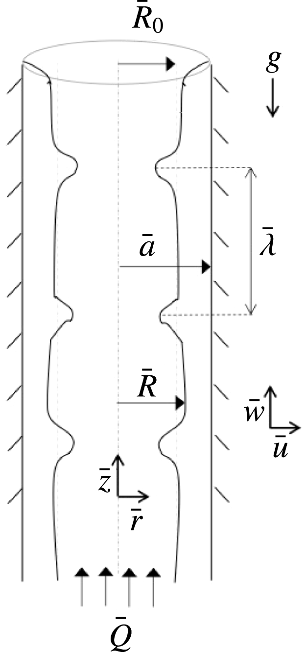
increases moving up the tube (see figure 1).
Variables definition sketch: core–annular flow in a vertical tube.

There is an exact Poiseuille-like solution to (2.1) where
 $\bar{u}^{(l,g)}=0$
,
 $\unicode[STIX]{x2202}_{\bar{z}}\bar{w}=0$
,
 $\unicode[STIX]{x2202}_{\bar{z}}\bar{p}=0$
, and the free surface is flat, i.e.
 $\bar{R}=\bar{R}_{0}$
,
 $$\begin{eqnarray}\displaystyle \bar{w}^{(l)} & = & \displaystyle \frac{\bar{r}^{2}-\bar{a}^{2}}{4\bar{\unicode[STIX]{x1D707}}^{(l)}}(\bar{p}_{\bar{z}}+\bar{\unicode[STIX]{x1D70C}}^{(l)}\bar{g})+\frac{\bar{g}\bar{R}_{0}^{2}}{2\bar{\unicode[STIX]{x1D707}}^{(l)}}(\bar{\unicode[STIX]{x1D70C}}^{(g)}-\bar{\unicode[STIX]{x1D70C}}^{(l)})\log \frac{\bar{r}}{\bar{a}},\quad \bar{R}\leqslant \bar{r}\leqslant \bar{a},\end{eqnarray}$$
 $$\begin{eqnarray}\displaystyle \bar{w}^{(g)} & = & \displaystyle \frac{\bar{r}^{2}-\bar{R}_{0}^{2}}{4\bar{\unicode[STIX]{x1D707}}^{(g)}}(\bar{p}_{\bar{z}}+\bar{\unicode[STIX]{x1D70C}}^{(g)}\bar{g})+\frac{\bar{R}_{0}^{2}-\bar{a}^{2}}{4\bar{\unicode[STIX]{x1D707}}^{(l)}}(\bar{p}_{\bar{z}}+\bar{\unicode[STIX]{x1D70C}}^{(l)}\bar{g})\nonumber\\ \displaystyle & & \displaystyle +\,\frac{\bar{g}\bar{R}_{0}^{2}}{2\bar{\unicode[STIX]{x1D707}}^{(l)}}(\bar{\unicode[STIX]{x1D70C}}^{(g)}-\bar{\unicode[STIX]{x1D70C}}^{(l)})\log \frac{\bar{R}_{0}}{\bar{a}},\quad \bar{a}\leqslant \bar{r}\leqslant 0.\end{eqnarray}$$
 $$\begin{eqnarray}\displaystyle \bar{w}^{(l)}(\bar{a}) & = & \displaystyle 0,\end{eqnarray}$$
 $$\begin{eqnarray}\displaystyle \bar{w}^{(l)}(\bar{R}) & = & \displaystyle \bar{w}^{(g)}(\bar{R}),\end{eqnarray}$$
 $$\begin{eqnarray}\displaystyle \bar{\unicode[STIX]{x1D707}}^{(l)}\unicode[STIX]{x2202}_{\bar{r}}\bar{w}^{(l)}|_{\bar{r}=\bar{R}} & = & \displaystyle \bar{\unicode[STIX]{x1D707}}^{(g)}\unicode[STIX]{x2202}_{\bar{r}}\bar{w}^{(g)}|_{\bar{r}=\bar{R}},\end{eqnarray}$$
 $\bar{r}=\bar{R}(\bar{z},\bar{t})$
, respectively. The stability of these exact solutions was studied by Hickox (Reference Hickox1971), who showed that while pipe flow of a single fluid is stable to infinitesimal perturbations, core–annular flow can be unstable to long-wave perturbations at any Reynolds number. His analysis was based on an adaptation of the long-wavenumber method developed by Yih (Reference Yih1967) for flat films where small linear disturbances to the velocities and pressure were expressed as asymptotic power series in wavenumber; by taking the small-wavenumber asymptotic limit, the propagation speed of an infinitesimal disturbance is determined at zeroth order, and its linear stability at first order (see also Goren Reference Goren1962, and Joseph & Renardy Reference Joseph and Renardy1993, for the stability analysis of related problems).
In the presence of long-wave disturbances, there is an approximate solution which is a slowly varying
 $\bar{z}$
-dependent modulation of the exact parallel flow; replacing
 $\bar{R}_{0}$
in (2.2) with
 $\bar{R}(\bar{z},\bar{t})$
results in this ‘long-wave’ flow (see Camassa & Ogrosky (Reference Camassa and Ogrosky2015) for a full derivation). This slowly varying solution (2.2a
) for the annular liquid is the backbone of the locally Poiseuille model derived in Camassa et al. (Reference Camassa, Forest, Lee, Ogrosky and Olander2012). Of course, when the core fluid flow is turbulent, the solution (2.2b
) is not expected to be a good representation of the core flow, and the stresses exerted on the annular film at the free surface by this turbulent flow demand modification of (2.2a
) as well. In the locally Poiseuille approach, this modification took the form of an effective viscosity based on a zero-equation turbulence closure model (White Reference White1991).
Since the velocity of the air is several orders of magnitude larger than the velocity of the liquid in the parameter ranges considered here, it can be assumed that the airflow experiences the free surface essentially as a rigid wavy wall. Before modelling the liquid flow through a modification of (2.2a ), we first study the airflow separately to model the stresses the airflow creates at the free surface. These stresses will be estimated next for both airflow through a wavy channel and through a wavy pipe.
3 Modelling airflow in a wavy channel
In this section, a model is developed for the wall stresses created by turbulent airflow through a wavy channel, and a comparison is made with previous experiments and models. As the fluid considered here is air, gravity is neglected in the model derivation, and we begin by stating the governing equations for a horizontally aligned channel.
3.1 Problem set-up
Consider the turbulent flow of air through a wavy channel with mean channel half-width
 $\bar{L}_{0}$
and local half-width
 $\bar{L}(\bar{z})=\bar{L}_{0}+\bar{\unicode[STIX]{x1D6FC}}(\bar{z})$
. The time-averaged flow is governed by the incompressible Reynolds-averaged Navier–Stokes (RANS) equations
 $$\begin{eqnarray}\displaystyle \bar{\unicode[STIX]{x1D70C}}^{(g)}(\bar{U}\bar{U}_{\bar{x}}+\bar{W}\bar{U}_{\bar{z}}) & = & \displaystyle -\bar{P}_{\bar{x}}+\bar{\unicode[STIX]{x1D707}}^{(g)}\bar{U}_{\bar{x}\bar{x}}+\bar{\unicode[STIX]{x1D707}}^{(g)}\bar{U}_{\bar{z}\bar{z}}+\bar{\unicode[STIX]{x1D70F}}_{11\bar{x}}+\bar{\unicode[STIX]{x1D70F}}_{12\bar{z}},\end{eqnarray}$$
 $$\begin{eqnarray}\displaystyle \bar{\unicode[STIX]{x1D70C}}^{(g)}(\bar{U}\bar{W}_{\bar{x}}+\bar{W}\bar{W}_{\bar{z}}) & = & \displaystyle -\bar{P}_{\bar{z}}+\bar{\unicode[STIX]{x1D707}}^{(g)}\bar{W}_{\bar{x}\bar{x}}+\bar{\unicode[STIX]{x1D707}}^{(g)}\bar{W}_{\bar{z}\bar{z}}+\bar{\unicode[STIX]{x1D70F}}_{12\bar{x}}+\bar{\unicode[STIX]{x1D70F}}_{22\bar{z}},\end{eqnarray}$$
 $$\begin{eqnarray}\displaystyle \bar{U}_{\bar{x}}+\bar{W}_{\bar{z}} & = & \displaystyle 0,\end{eqnarray}$$
 $(\bar{U},\bar{W})$
are the time-averaged velocity components in the
 $(\bar{x},\bar{z})$
directions,
 $\bar{P}$
is the time-averaged pressure and
 $\bar{\unicode[STIX]{x1D70F}}_{ij}$
are the components of the Reynolds stress tensor;
 $\bar{\unicode[STIX]{x1D70C}}^{(g)}$
is the density and
 $\bar{\unicode[STIX]{x1D707}}^{(g)}$
is the dynamic viscosity. Letter subscripts denote partial derivatives and bars denote dimensional quantities. Here
 $\bar{z}$
increases as one moves downstream and
 $\bar{x}$
increases as one moves outward from the centre of the channel, so that
 $\bar{x}=\bar{L}(\bar{z})$
corresponds to the wavy wall and
 $\bar{x}=0$
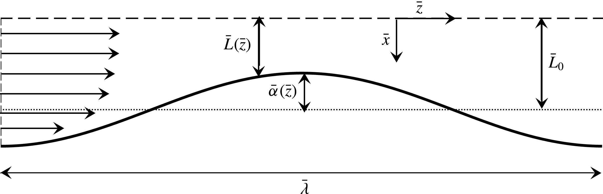
corresponds to the centre of the channel; see figure 2 for a definition sketch of the flow variables. Boundary conditions at the wall
 $\bar{x}=\bar{L}(\bar{z})$
are no slip,
 $$\begin{eqnarray}\displaystyle \bar{U}=\bar{W}=0, & & \displaystyle\end{eqnarray}$$
and at the centre of the channel
 $\bar{x}=0$
we require that
 $$\begin{eqnarray}\displaystyle \bar{W}_{\bar{x}}=0. & & \displaystyle\end{eqnarray}$$
Variables definition sketch for wavy channel flow.

Next, the problem can be non-dimensionalized by the following reference scales:
 $$\begin{eqnarray}\displaystyle \left.\begin{array}{@{}c@{}}\displaystyle x=\bar{x}/\bar{L}_{C},\quad z=\unicode[STIX]{x1D716}_{C}\bar{z}/\bar{L}_{C},\quad U=\bar{U}/\unicode[STIX]{x1D716}_{C}\bar{W}_{C},\\ \quad W=\bar{W}/\bar{W}_{C},\quad P=\unicode[STIX]{x1D716}_{C}\bar{P}/|\bar{T}_{C}|,\quad \unicode[STIX]{x1D70F}=\bar{\unicode[STIX]{x1D70F}}/|\bar{T}_{C}|,\end{array}\right\} & & \displaystyle\end{eqnarray}$$
where
 $\unicode[STIX]{x1D716}_{C}=\bar{L}_{0}/\bar{\unicode[STIX]{x1D706}}$
is an aspect ratio, the velocity scale
 $$\begin{eqnarray}\displaystyle \bar{W}_{C}=\frac{\bar{Q}_{C}}{2\bar{L}_{0}}\sqrt{\frac{F_{C}}{2}}, & & \displaystyle\end{eqnarray}$$
is the friction velocity estimated using the empirical skin friction coefficient
 $$\begin{eqnarray}\displaystyle F_{C}=0.073(Re_{C}^{(g)})^{-0.25},\quad Re_{C}^{(g)}=\frac{\bar{\unicode[STIX]{x1D70C}}^{(g)}\bar{Q}_{C}}{2\bar{\unicode[STIX]{x1D707}}^{(g)}}, & & \displaystyle\end{eqnarray}$$
and where
 $Re_{C}^{(g)}$
is the bulk Reynolds number and
 $\bar{Q}_{C}$
is the prescribed area flux of air. Subscripts of
 $C$
are used to denote the case of channel flow in order to avoid confusion with the analogous quantities defined for pipe flow in § 4. Note that the bulk Reynolds number and skin friction coefficient do not depend on the average channel half-width
 $\bar{L}_{0}$
, but only on the fluid properties and flux
 $\bar{Q}_{C}$
. The length and stress/pressure scales are
 $$\begin{eqnarray}\displaystyle \bar{L}_{C}=\frac{\bar{\unicode[STIX]{x1D707}}^{(g)}}{\bar{\unicode[STIX]{x1D70C}}^{(g)}\bar{W}_{C}},\quad |\bar{T}_{C}|=\bar{\unicode[STIX]{x1D70C}}^{(g)}(\bar{W}_{C})^{2}=\frac{\bar{\unicode[STIX]{x1D70C}}^{(g)}F_{C}\bar{Q}_{C}^{2}}{8\bar{L}_{0}^{2}}. & & \displaystyle\end{eqnarray}$$
Here
 $|\bar{T}_{C}|$
is an empirical estimate of the wall stress in flow through a flat channel of half-width
 $\bar{L}_{0}$
. Thus, given the ‘hardware’ parameters
 $\bar{L}_{0}$
,
 $\bar{\unicode[STIX]{x1D706}}$
,
 $\bar{Q}_{C}$
,
 $\bar{\unicode[STIX]{x1D707}}^{(g)}$
and
 $\bar{\unicode[STIX]{x1D70C}}^{(g)}$
, i.e. parameters that are a fixed property of the fluid or geometry (as opposed to parameters and scalings selected by initial conditions), all scales of the problem are determined. We note that recent studies have shown that liquid-infused porous surfaces are able to reduce the skin friction; drag reduction has been demonstrated for both turbulent and laminar flow (see, e.g. Solomon, Khalil & Varanasi (Reference Solomon, Khalil and Varanasi2014) and Rosenberg et al. (Reference Rosenberg, Van Buren, Fu and Smits2016), respectively).
Using this scaling, the dimensionless wall is given by
 $x=L(z)=L_{0}+\unicode[STIX]{x1D6FC}(z)$
, where
 $L_{0}=\bar{L}_{0}/\bar{L}_{C}$
is the dimensionless channel width and
 $\unicode[STIX]{x1D6FC}=\bar{\unicode[STIX]{x1D6FC}}/\bar{L}_{C}$
measures the local constriction of the channel;
 $\unicode[STIX]{x1D6FC}(z)<0$
indicates a narrow region of the channel while
 $\unicode[STIX]{x1D6FC}(z)>0$
indicates a relatively wide region of the channel. Substituting (3.4) into (3.1) results in
 $$\begin{eqnarray}\displaystyle \unicode[STIX]{x1D716}_{C}^{3}(UU_{x}+WU_{z}) & = & \displaystyle -P_{x}+\unicode[STIX]{x1D716}_{C}^{2}U_{xx}+\unicode[STIX]{x1D716}_{C}^{4}U_{zz}+\unicode[STIX]{x1D716}_{C}\unicode[STIX]{x1D70F}_{11x}+\unicode[STIX]{x1D716}_{C}^{2}\unicode[STIX]{x1D70F}_{12z},\end{eqnarray}$$
 $$\begin{eqnarray}\displaystyle \unicode[STIX]{x1D716}_{C}(UW_{x}+WW_{z}) & = & \displaystyle -P_{z}+W_{xx}+\unicode[STIX]{x1D716}_{C}^{2}W_{zz}+\unicode[STIX]{x1D70F}_{12x}+\unicode[STIX]{x1D716}_{C}\unicode[STIX]{x1D70F}_{22z},\end{eqnarray}$$
 $$\begin{eqnarray}\displaystyle U_{x}+W_{z} & = & \displaystyle 0.\end{eqnarray}$$
3.2 Coordinate transformation
Analysis in the usual Cartesian coordinates is difficult and, as previous studies have demonstrated, significant simplifications and improved agreement with experiments can arise if a curvilinear coordinate system is used instead. We move to a coordinate system which ‘flattens’ the wavy channel; the base flow in this flattened channel is estimated by using an effective viscosity approximated by a simple mixing-length model. This approach is similar to that used by, e.g. Benjamin (Reference Benjamin1959) and Tseluiko & Kalliadasis (Reference Tseluiko and Kalliadasis2011), but is not equivalent: here, a ‘long-wave’ approximation will be made from the outset, i.e.
 $$\begin{eqnarray}\displaystyle \unicode[STIX]{x1D716}_{C}\ll 1. & & \displaystyle\end{eqnarray}$$
This results in a base flow slowly modulated in the
 $z$
direction to take into account the channel’s local half-width. This slowly modulated base flow is analogous to the base flow used in the locally Poiseuille modelling approach of Camassa et al. (Reference Camassa, Forest, Lee, Ogrosky and Olander2012) and is used here to estimate first-order corrections to the wall stress.
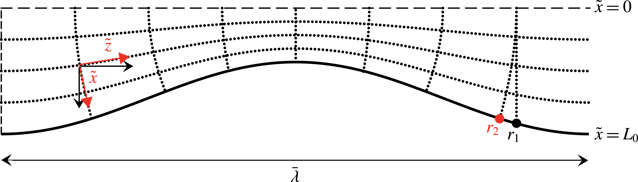
Gridlines in the curvilinear coordinate system
 $(\tilde{x},\tilde{z})$
for flow through a wavy channel. Local basis vectors are depicted for Cartesian coordinates (black) and curvilinear coordinates (red) at one point. Points
 $r_{1}$
and
 $r_{2}$
are discussed in the text.

We undertake a coordinate transformation
 $(x,z)\rightarrow (\tilde{x},\tilde{z})$
, where we define
 $$\begin{eqnarray}\displaystyle \tilde{x}=\frac{L_{0}}{L(z)}x, & & \displaystyle\end{eqnarray}$$
so that
 $\tilde{x}=L_{0}$
is coincident with the wavy wall
 $x=L(z)$
,
 $\tilde{x}=0$
is coincident with the centre of the tube
 $x=0$
, and curves of constant
 $\tilde{x}$
are relaxed linearly to the Cartesian coordinate system as one moves away from the wall to the centre of the channel. The curves of constant
 $\tilde{z}$
are then defined so that they are orthogonal to curves of constant
 $\tilde{x}$
; see figure 3. The linear relaxation of the curves of constant
 $\tilde{x}$
lies somewhat between the exponential relaxation of these curves used by Benjamin (Reference Benjamin1959) and Tseluiko & Kalliadasis (Reference Tseluiko and Kalliadasis2011), and the lack of any relaxation used by Thorsness et al. (Reference Thorsness, Morrisroe and Hanratty1978). Tildes will denote the new coordinate system throughout this section; subscripts of
 $1$
or
 $2$
denote components in the
 $\tilde{x}$
or
 $\tilde{z}$
direction, respectively (or in the
 $x$
or
 $z$
direction, respectively, depending on the context).
Given the long-wave approximation
 $\unicode[STIX]{x1D716}_{C}\ll 1$
, the partial derivatives with respect to
 $x$
and
 $z$
and the Laplacian
 $\unicode[STIX]{x0394}\equiv \unicode[STIX]{x1D6FB}^{2}$
are expressed in the new coordinate system by (A 1) and (A 2) in appendix A, respectively; likewise, the velocities
 $(U,W)$
and Reynolds stresses
 $\unicode[STIX]{x1D70F}_{ij}$
can be transformed into
 $(\tilde{U} ,\tilde{W})$
and
 $\tilde{\unicode[STIX]{x1D70F}}_{ij}$
, respectively, according to (A 3). Each of these flow variables in the new coordinate system can then be expanded in the small parameter
 $\unicode[STIX]{x1D716}_{C}$
,
 $$\begin{eqnarray}\displaystyle \tilde{U} (x,z) & = & \displaystyle \tilde{U} _{0}(\tilde{x},\tilde{z})+\unicode[STIX]{x1D716}_{C}\tilde{U} _{1}(\tilde{x},\tilde{z})+O(\unicode[STIX]{x1D716}_{C}^{2}),\end{eqnarray}$$
 $$\begin{eqnarray}\displaystyle \tilde{W}(x,z) & = & \displaystyle \tilde{W}_{0}(\tilde{x},\tilde{z})+\unicode[STIX]{x1D716}_{C}\tilde{W}_{1}(\tilde{x},\tilde{z})+O(\unicode[STIX]{x1D716}_{C}^{2}),\end{eqnarray}$$
 $$\begin{eqnarray}\displaystyle \tilde{P}(x,z) & = & \displaystyle \tilde{P}_{0}(\tilde{x},\tilde{z})+\unicode[STIX]{x1D716}_{C}\tilde{P}_{1}(\tilde{x},\tilde{z})+O(\unicode[STIX]{x1D716}_{C}^{2}),\end{eqnarray}$$
 $$\begin{eqnarray}\displaystyle \tilde{\unicode[STIX]{x1D70F}}_{ij}(x,z) & = & \displaystyle \tilde{\unicode[STIX]{x1D70F}}_{ij_{0}}(\tilde{x},\tilde{z})+\unicode[STIX]{x1D716}_{C}\tilde{\unicode[STIX]{x1D70F}}_{ij_{1}}(\tilde{x},\tilde{z})+O(\unicode[STIX]{x1D716}_{C}^{2}).\end{eqnarray}$$
The essence of the locally Poiseuille approach in Camassa et al. (Reference Camassa, Forest, Lee, Ogrosky and Olander2012) is to seek velocity solutions whose leading-order components satisfy
 $$\begin{eqnarray}\displaystyle \tilde{U} _{0}(\tilde{x},\tilde{z})=0,\quad \tilde{W}_{0}(\tilde{x},\tilde{z}) & = & \displaystyle \tilde{w}_{0}(\tilde{x})g_{0}(\tilde{z}),\end{eqnarray}$$
so that the leading-order velocity profile in the new coordinate system is a parallel flow whose speed is modulated by the wall waviness present in the Cartesian coordinate system. We now make one further assumption, that the normal Reynolds stresses are
 $O(\unicode[STIX]{x1D716}_{C})$
, i.e.
 $\tilde{\unicode[STIX]{x1D70F}}_{ii_{0}}=0$
for
 $i=1,2$
, and adopt a turbulent viscosity model for the Reynolds shear stress
 $\tilde{\unicode[STIX]{x1D70F}}_{12}$
, i.e.
 $$\begin{eqnarray}\displaystyle \tilde{\unicode[STIX]{x1D70F}}_{12_{0}}(\tilde{x},\tilde{z})=\tilde{\unicode[STIX]{x1D707}}^{\ast }(\tilde{x},\tilde{z})\tilde{w}_{0}^{\prime }\tilde{g}_{0}\frac{L_{0}}{L}, & & \displaystyle\end{eqnarray}$$
where primes denote
 $\text{d}/\text{d}\tilde{x}$
. It is assumed that the turbulent viscosity in this new coordinate system can be approximated by the mixing-length model,
 $$\begin{eqnarray}\displaystyle \tilde{\unicode[STIX]{x1D707}}^{\ast }(\tilde{x},\tilde{z}) & = & \displaystyle \frac{L}{L_{0}}[l_{C}(\tilde{x})]^{2}|\tilde{w}_{0}^{\prime }|\tilde{g}_{0},\end{eqnarray}$$
where
 $\tilde{g}_{0}$
is the
 $\tilde{z}$
-component of the leading-order streamwise velocity. The mixing length
 $l_{C}$
can be modelled by the van Driest equation,
 $$\begin{eqnarray}\displaystyle l_{C}(\tilde{x})=\unicode[STIX]{x1D705}(L_{0}-\tilde{x})[1-\exp ((\tilde{x}-L_{0})/A)], & & \displaystyle\end{eqnarray}$$
where
 $\unicode[STIX]{x1D705}\approx 0.41$
is von Kármán’s constant, and
 $A=26$
is a constant determined empirically (van Driest Reference van Driest1956; Bailey et al.
Reference Bailey, Vallikivi, Hultmark and Smits2014; Schlichting & Gersten Reference Schlichting and Gersten2017). While no mixing length model can adequately capture all flow features near the wall, and while various modifications have been proposed to this simple model, we elect to use the original formulation of van Driest due to its simplicity and ability to produce the main features of experimental flow near the wall over a wide range of Reynolds numbers (van Driest Reference van Driest1956).
3.3 Leading-order solution
Substitution of (A 1)–(A 3) and (3.11)–(3.15) into (3.8) and collection of the leading-order terms in
 $\unicode[STIX]{x1D716}_{C}$
results in
 $$\begin{eqnarray}\displaystyle \unicode[STIX]{x2202}_{\tilde{x}}\tilde{P}_{0} & = & \displaystyle 0,\end{eqnarray}$$
 $$\begin{eqnarray}\displaystyle \unicode[STIX]{x2202}_{\tilde{z}}\tilde{P}_{0} & = & \displaystyle \frac{\tilde{g}_{0}L_{0}^{2}}{L^{2}}\tilde{w}_{0}^{\prime \prime }+\frac{\tilde{g}_{0}^{2}L_{0}}{L}\frac{\text{d}}{\text{d}\tilde{x}}\left[l_{C}^{2}(\tilde{w}_{0}^{\prime })^{2}\right],\end{eqnarray}$$
 $$\begin{eqnarray}\displaystyle \left(\frac{\tilde{g}_{0}}{L}\frac{\text{d}L}{\text{d}\tilde{z}}+\frac{\text{d}\tilde{g}_{0}}{\text{d}\tilde{z}}\right)\tilde{w}_{0} & = & \displaystyle 0,\end{eqnarray}$$
 $\unicode[STIX]{x2202}_{\tilde{x}}\tilde{P}_{0}$
from (3.16b
), and where functional dependence has been omitted for brevity. Equations (3.16) are subject to the boundary conditions
 $$\begin{eqnarray}\displaystyle \tilde{w}_{0}=0 & & \displaystyle \text{at }\tilde{x}=L_{0},\end{eqnarray}$$
 $$\begin{eqnarray}\displaystyle \tilde{w}_{0}^{\prime }=0 & & \displaystyle \text{at }\tilde{x}=0.\end{eqnarray}$$
Equation (3.16) is satisfied by
 $$\begin{eqnarray}\displaystyle \tilde{g}_{0}=\frac{L_{0}}{L},\quad \unicode[STIX]{x2202}_{\tilde{z}}\tilde{P}_{0}=-\frac{L_{0}^{2}}{L^{3}}. & & \displaystyle\end{eqnarray}$$
The
 $\tilde{x}$
component of the leading-order streamwise velocity, i.e.
 $\tilde{w}_{0}$
, can then be found by solving
 $$\begin{eqnarray}\displaystyle -\frac{1}{L_{0}} & = & \displaystyle \tilde{w}_{0}^{\prime \prime }+\frac{\text{d}}{\text{d}\tilde{x}}[l_{C}^{2}(\tilde{w}_{0}^{\prime })^{2}],\end{eqnarray}$$
which, after integrating once, is a straightforward quadratic equation in
 $\tilde{w}_{0}^{\prime }$
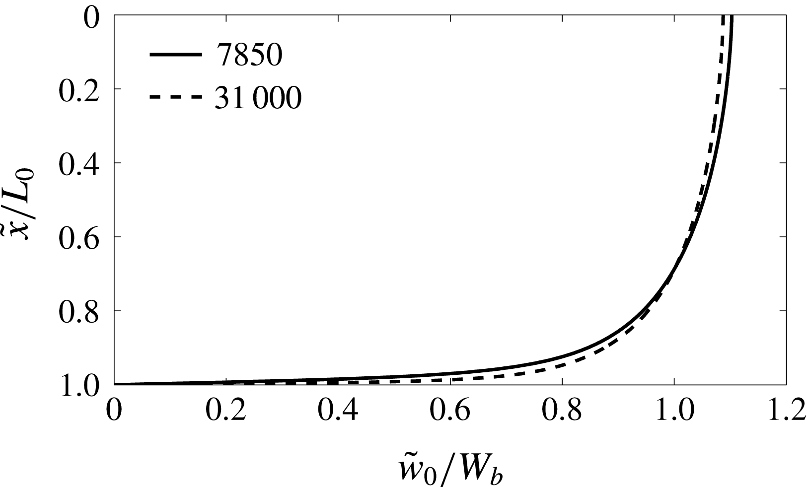
which can be solved and integrated numerically using boundary conditions (3.17) to give the leading-order velocity profile. Figure 4 shows the velocity profile for two different Reynolds numbers. We remark again that in flows through a wavy channel the Reynolds number, and hence the skin friction coefficient, does not vary as the local channel half-width varies. This velocity profile thus forms a set of self-similar solutions that create wall stresses identical to those of the laminar solutions used with an effective viscosity in Camassa et al. (Reference Camassa, Forest, Lee, Ogrosky and Olander2012). This leading-order wall stress is given by
 $$\begin{eqnarray}\displaystyle \bar{\unicode[STIX]{x1D70F}}_{C_{0}}^{(g)} & = & \displaystyle -|\bar{T}_{C}|\frac{L_{0}^{2}}{L^{2}},\end{eqnarray}$$
and will be referred to as the locally Poiseuille (LP) model for the wall stress.
Leading-order streamwise velocity profile
 $\tilde{w}_{0}$
in (3.19) for channel airflow with
 $Re_{C}^{(g)}=7850$
and
 $Re_{C}^{(g)}=31\,000$
.
 $W_{b}=1/\bar{L}_{0}\int _{0}^{\bar{L}_{0}}\tilde{w}_{0}(x)\,\text{d}x$
denotes the bulk velocity.

3.4 First-order corrections
We next extend the locally Poiseuille approach to include first-order corrections. Due to the aspect ratio assumptions made, only the streamwise velocity corrections
 $\tilde{W}_{1}(\tilde{x},\tilde{z})$
are necessary for estimating the wall shear stress to
 $O(\unicode[STIX]{x1D716}_{C})$
, and so we include only those steps needed for estimating this term.
Similar to the leading-order component, we seek a streamwise velocity correction of the form
 $$\begin{eqnarray}\displaystyle \tilde{W}_{1}(\tilde{x},\tilde{z})=\tilde{w}_{1}(\tilde{x})\tilde{g}_{1}(\tilde{z}). & & \displaystyle\end{eqnarray}$$
Substitution of (3.21) into the momentum equations and collecting terms of
 $O(\unicode[STIX]{x1D716}_{C})$
results in
 $$\begin{eqnarray}\displaystyle \unicode[STIX]{x2202}_{\tilde{x}}\tilde{P}_{1} & = & \displaystyle 0,\end{eqnarray}$$
 $$\begin{eqnarray}\displaystyle -\!\frac{L_{0}^{2}}{L^{3}}\frac{\text{d}L}{\text{d}\tilde{z}}\tilde{w}_{0}^{2} & = & \displaystyle -\unicode[STIX]{x2202}_{\tilde{z}}\tilde{P}_{1}+\frac{\tilde{g}_{1}L_{0}^{2}}{L^{2}}\left[\tilde{w}_{1}^{\prime \prime }+2\frac{\text{d}}{\text{d}\tilde{x}}(l^{2}\tilde{w}_{1}^{\prime }\tilde{w}_{0}^{\prime })\right].\end{eqnarray}$$
 $\tilde{U} _{1}(\tilde{x},\tilde{z})$
by
 $x$
-integration of the velocity shear
 $\unicode[STIX]{x2202}_{z}\tilde{W}_{1}$
.)
The
 $\tilde{z}$
-component
 $\tilde{g}_{1}$
of the streamwise velocity corrections can be found by first integrating (3.22b
) across the channel half-width resulting in
 $$\begin{eqnarray}\displaystyle \unicode[STIX]{x2202}_{\tilde{z}}\tilde{P}_{1} & = & \displaystyle \frac{L_{0}A_{C}}{L^{3}}\frac{\text{d}L}{\text{d}\tilde{z}}+\frac{\tilde{g}_{1}L_{0}B_{C}}{L^{2}},\end{eqnarray}$$
with
 $$\begin{eqnarray}\displaystyle A_{C}=\int _{0}^{L_{0}}\tilde{w}_{0}^{2}\,\text{d}\tilde{x},\quad B_{C}=\unicode[STIX]{x2202}_{\tilde{x}}\tilde{w}_{1}|_{\tilde{x}=L_{0}}. & & \displaystyle\end{eqnarray}$$
Thus
 $A_{C}$
is a known constant obtained by numerically integrating the inertial terms across the channel, and
 $B_{C}$
is the wall stress correction term for which we seek an approximation. Substituting (3.23) into (3.22b
) gives
 $$\begin{eqnarray}\displaystyle -\!\frac{L_{0}^{2}}{L^{3}}\frac{\text{d}L}{\text{d}\tilde{z}}\left(\tilde{w}_{0}^{2}+\frac{A_{C}}{L_{0}}\right) & = & \displaystyle \frac{\tilde{g}_{1}L_{0}^{2}}{L^{2}}\left(\tilde{w}_{1}^{\prime \prime }+2\frac{\text{d}}{\text{d}\tilde{x}}[l_{C}^{2}(\tilde{w}_{1}^{\prime })(\tilde{w}_{0}^{\prime })]-\frac{B_{C}}{L_{0}}\right),\end{eqnarray}$$
and so we set
 $$\begin{eqnarray}\displaystyle \tilde{g}_{1}(\tilde{z})=\frac{1}{L}\frac{\text{d}L}{\text{d}\tilde{z}}. & & \displaystyle\end{eqnarray}$$
The
 $\tilde{x}$
-component
 $\tilde{w}_{1}$
of the streamwise velocity gradient corrections can be found in terms of the unknown pressure gradient correction
 $\unicode[STIX]{x2202}_{\tilde{z}}\tilde{P}_{1}$
by integrating equation (3.25) once and applying the zero shear condition at the centre of the tube;
 $\tilde{w}_{1}$
can then be found in terms of
 $\unicode[STIX]{x2202}_{\tilde{z}}\tilde{P}_{1}$
by integrating the equation a second time while applying the no-slip condition at the wall. The resulting velocity profile
 $\tilde{w}_{1}$
may be integrated across the channel from
 $\tilde{x}=0$
to
 $\tilde{x}=L_{0}$
; this integral must be set to zero by selection of the pressure gradient correction
 $\unicode[STIX]{x2202}_{\tilde{z}}\tilde{P}_{1}$
(or equivalently selection of
 $B_{C}$
) since the leading-order profile accounts entirely for the prescribed constant volume flux. The resulting dimensional first-order wall stress corrections are
 $$\begin{eqnarray}\displaystyle \bar{\unicode[STIX]{x1D70F}}_{C_{1}}^{(g)} & = & \displaystyle |\bar{T}_{C}|\frac{\bar{L}_{0}^{2}}{\bar{L}^{2}}\frac{\text{d}\bar{L}}{\text{d}\bar{z}}B_{C}^{\ast },\end{eqnarray}$$
where
 $$\begin{eqnarray}\displaystyle B_{C}^{\ast }=\frac{\bar{L}_{C}}{\bar{L}_{0}}B_{C}=\sqrt{\frac{2}{0.079}}(Re_{C}^{(g)})^{7/8}B_{C}. & & \displaystyle\end{eqnarray}$$
Having found the first-order stress corrections, the total shear stress up to
 $O(\unicode[STIX]{x1D716}_{C})$
may be expressed in dimensional form as
 $\bar{\unicode[STIX]{x1D70F}}_{C}^{(g)}=\bar{\unicode[STIX]{x1D70F}}_{C_{0}}^{(g)}+\bar{\unicode[STIX]{x1D70F}}_{C_{1}}^{(g)}$
,
 $$\begin{eqnarray}\displaystyle \bar{\unicode[STIX]{x1D70F}}_{C}^{(g)} & = & \displaystyle |\bar{T}_{C}|\left(\frac{\bar{L}_{0}}{\bar{L}}\right)^{2}\left[-1+B_{C}^{\ast }\frac{\text{d}\bar{L}}{\text{d}\bar{z}}\right].\end{eqnarray}$$
The first term in (3.29), i.e. the leading-order stress, represents the modelled stress found using the LP model in Camassa et al. (Reference Camassa, Forest, Lee, Ogrosky and Olander2012) (adapted here for channel flow). The second term represents the first-order corrections, and we will refer to the total stress (3.29) as the first-order or long-wave model. The locally Poiseuille stress is in phase with the wall while the first-order stress (3.29) depends both on the wall and its gradient. The dimensional normal stresses at the wall, up to
 $O(\unicode[STIX]{x1D716}_{C})$
, are given by
 $$\begin{eqnarray}\displaystyle \unicode[STIX]{x2202}_{\bar{z}}\bar{P}_{C}^{(g)} & = & \displaystyle \frac{|\bar{T}_{C}|}{\bar{L}_{0}}\left(\frac{\bar{L}_{0}}{\bar{L}}\right)^{3}\left[-1+(B_{C}+A_{C})\frac{\bar{L}_{C}}{\bar{L}_{0}}\frac{\text{d}\bar{L}}{\text{d}\bar{z}}\right].\end{eqnarray}$$
The coefficients
 $A_{C}$
and
 $B_{C}^{\ast }$
are numerically determined functions of the gas Reynolds number
 $Re_{C}^{(g)}$
defined in (3.6).
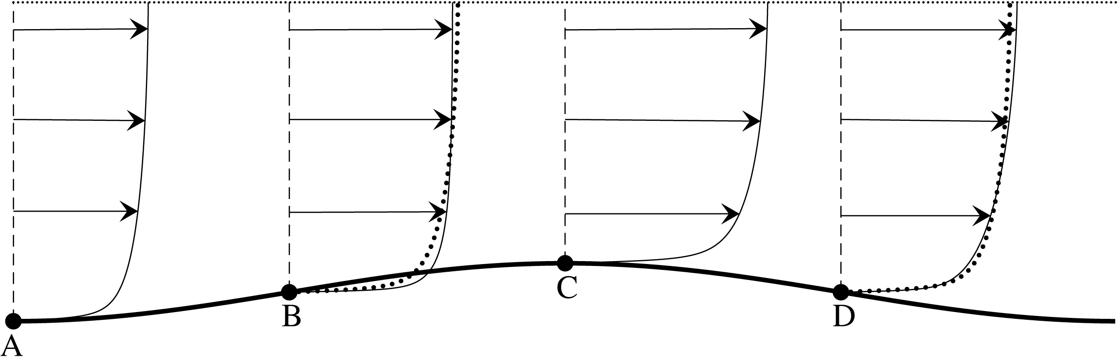
Streamwise velocity profile for first-order (solid lines) and leading-order (dotted lines) models along one wavelength of a wavy channel (figure not to scale).

A sketch of the streamwise velocity profile with first-order corrections for a small-amplitude wavy wall is shown in figure 5. At locations where the wall gradient vanishes, i.e.
 $\text{d}\bar{L}/\text{d}\bar{z}=0$
, the velocity profile is the base profile modulated by the channel width; e.g. the velocity profile at points A and C are identical up to a factor of
 $\bar{L}(\bar{z}_{A})/\bar{L}(\bar{z}_{C})$
. In regions where the channel is constricting, e.g. point B where
 $\text{d}\bar{L}/\text{d}\bar{z}<0$
, the air flows faster near the walls and slower at the centre of the channel than it would due to the base profile alone; where the channel widens, e.g. point D where
 $\text{d}\bar{L}/\text{d}\bar{z}>0$
, the opposite holds. Thus constriction results in larger wall stress while widening results in smaller wall stress than that due to the base flow.
In the case of larger-amplitude wavy deformations of flat walls, and in the regions where the airflow is being constricted, i.e.
 $\text{d}\bar{L}/\text{d}\bar{z}<0$
, the maximum streamwise velocity occurs at a point close to the wall (not shown in figure 5). This behaviour is likely unphysical and was not seen in pipe and channel flow experiments, see, e.g. Hsu & Kennedy (Reference Hsu and Kennedy1971). We note that the same behaviour occurs in the model derived by Tseluiko & Kalliadasis (Reference Tseluiko and Kalliadasis2011) which exploits an assumed small amplitude of wall deformations – we thus refer hereafter to this model as a small-amplitude model – though the minimum amplitude required to produce this behaviour is much larger than in the first-order model. Nevertheless, our focus here is on whether the first-order model accurately captures the near-wall behaviour, and in particular the wall stress; this behaviour is considered next.
3.5 Comparison with experiments and other models
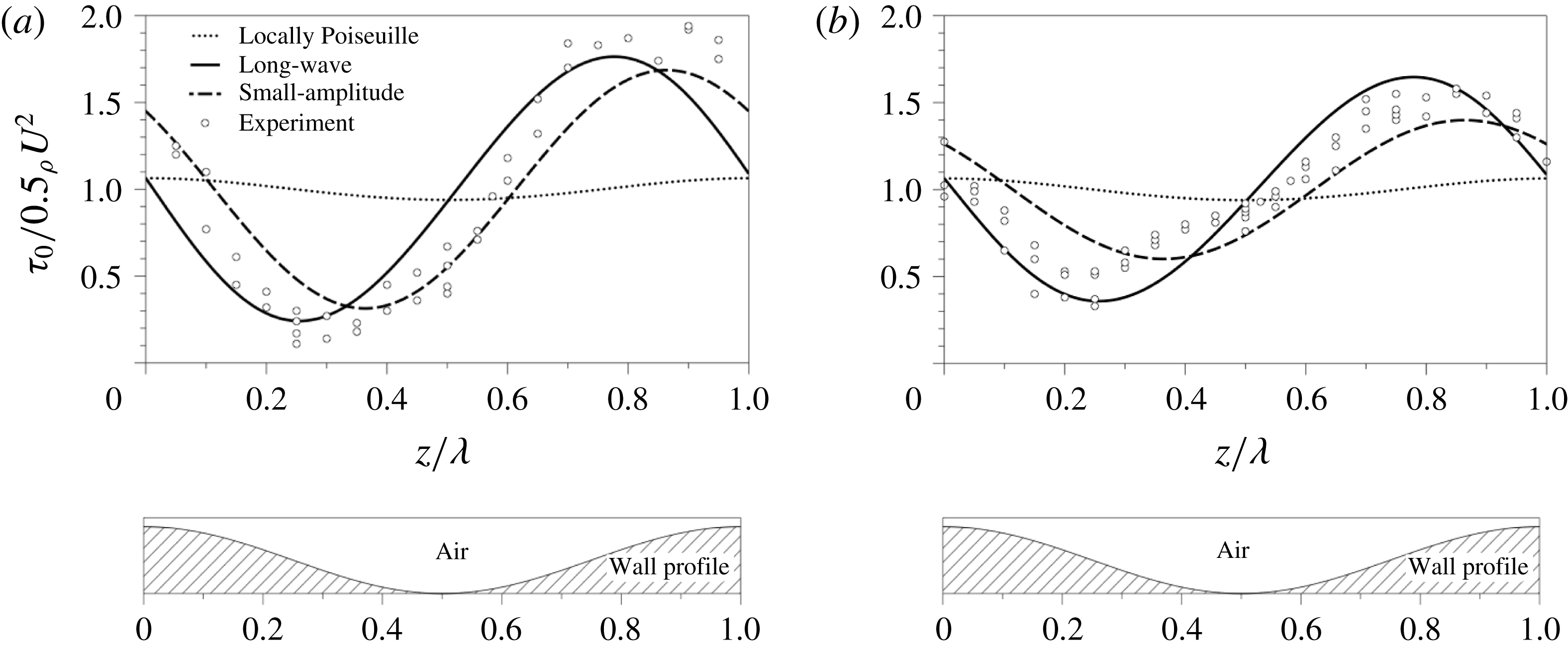
We now compare the first-order wall stress estimate (3.29) with both the leading-order locally Poiseuille estimate and the small-amplitude model of Tseluiko & Kalliadasis (Reference Tseluiko and Kalliadasis2011), as well as experiments reported in Zilker et al. (Reference Zilker, Cook and Hanratty1977). Figure 6 shows results for increasing Reynolds number with fixed wall wave amplitude of 0.079 cm (crest-to-trough amplitude 0.157 cm) and wavelength 5.08 cm in a channel with half-width 2.54 cm. Both the small-amplitude model and first-order model (3.29) match the experimental trend of smaller corrections relative to the magnitude of the leading-order stress for increasing Reynolds number. For the higher Reynolds number,
 $Re=31\,000$
, the first-order estimate (3.29) appears to capture both the phase shift and amplitude of the waviness-induced wall stress at least as well as the small-amplitude model and much better than the locally Poiseuille model. For the lower Reynolds number,
 $Re=7850$
, the small-amplitude model appears to slightly underestimate the phase shift; the first-order model slightly overestimates the phase shift. Both underestimate the amplitude of the waviness-induced stress; both models give much better agreement than the locally Poiseuille model.
Wall stress along one wavelength of a wavy channel predicted by the long-wave model (solid lines), locally Poiseuille model (dotted lines), small-amplitude model of Tseluiko & Kalliadasis (Reference Tseluiko and Kalliadasis2011) (dashed lines) and found in experiments of Zilker et al. (Reference Zilker, Cook and Hanratty1977) (circles) through a channel with half-width
 $\bar{L}_{0}=2.54~\text{cm}$
and a sinusoidally wavy wall with crest-to-trough amplitude 0.157 cm and wavelength 5.08 cm; the ratio of amplitude to wavelength has been enlarged in the wavy wall shown in the bottom panels. (a)
 $Re_{C}^{(g)}=7850$
, (b)
 $Re_{C}^{(g)}=31\,000$
; compare to figures 8 and 9 in Tseluiko & Kalliadasis (Reference Tseluiko and Kalliadasis2011) and figure 6 in Zilker et al. (Reference Zilker, Cook and Hanratty1977).

We note that the long-wave aspect ratio assumption used in deriving the stress estimates may not be strictly valid in the experiments of Zilker et al. (Reference Zilker, Cook and Hanratty1977), for which
 $\unicode[STIX]{x1D716}_{C}=L_{0}/\unicode[STIX]{x1D706}\approx 0.5$
. The reasonable agreement with experiments suggests, however, that the combination of terms neglected in the modelling may have only a small net contribution to the wall shear stress.
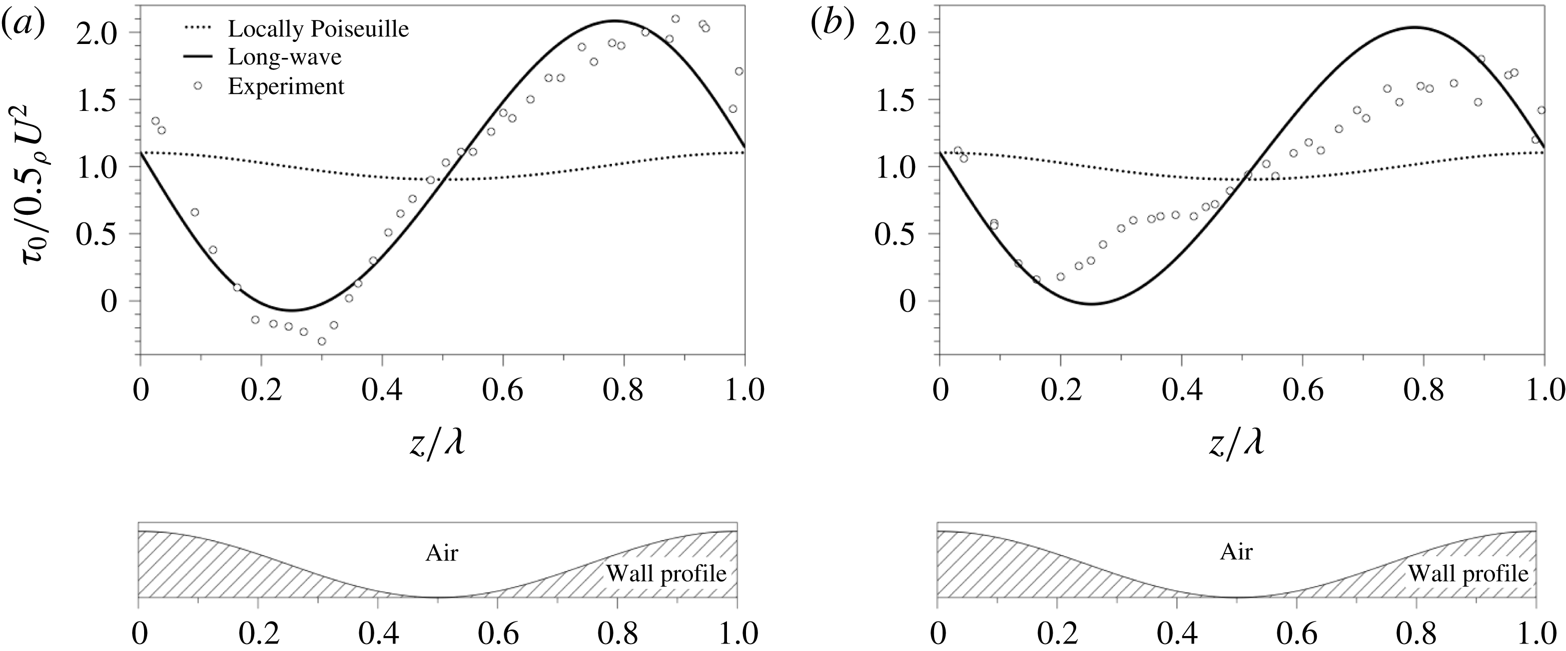
We next focus on the long-wave model for higher-amplitude wall perturbations; figure 7 shows results for increasing Reynolds number with fixed wall wave amplitude of 0.127 cm (crest-to-trough amplitude 0.254 cm) and wavelength 5.08 cm. The first-order model again exhibits the experimental trend of higher corrections relative to the magnitude of the leading-order stress for increased wave amplitude (a trend also seen in the small-amplitude model). In addition, the first-order model exhibits a small phase shift as the Reynolds number increases (a trend not present in the small-amplitude model). For the smaller Reynolds number, the first-order model estimates the amplitude of the corrections well; for the higher Reynolds number, the first-order model appears to overestimate the amplitude while also not accurately capturing the phase shift.
The experiments in figure 7 also show that if the wall waviness has large enough amplitude, the wall stress is nonlinear even for a sinusoidal wall profile. For example, in figure 7(b), the minimum reported experimental wall stress occurs at
 $x/\unicode[STIX]{x1D706}\approx 0.15$
and the maximum occurs at
 $x/\unicode[STIX]{x1D706}\approx 0.85$
; in contrast, a linear wall stress would have extrema located at 0.5 wavelengths apart. This effect is of course not captured in the small-amplitude model which neglects nonlinear interactions in velocity perturbations. The first-order model, through the dependence of
 $\unicode[STIX]{x1D70F}^{(g)}$
on
 $1/\bar{L}^{2}$
, displays this nonlinear behaviour, albeit very slightly, in qualitative agreement with experiments, i.e. the distance between the location of the model wall stress minimum and maximum in figure 7(b) is greater than 0.5 wavelengths. This nonlinear behaviour can be more readily seen in the results for wavy pipe flow in § 4.
It is also notable that in the experiments seen in figure 7(a) a region of negative wall stress was observed; the first-order model does not capture this behaviour in these figures, but does display this behaviour for smaller Reynolds number (not shown). It is important to note that the first-order model was derived under the assumption that the ratio of the characteristic velocity scales in the transverse and streamwise directions was small,
 $\bar{u}_{c}=\unicode[STIX]{x1D716}_{C}\bar{w}_{c}$
. In these regions of negative stress this assumption is clearly violated, as the negative shear stress indicates regions of air recirculation along the wavy wall troughs. However, as is frequently the case with asymptotics, the asymptotic formula (3.29) appears to have validity outside of the range of strict asymptotic derivation for small
 $\unicode[STIX]{x1D716}_{C}$
values.
Same as figure 6 but with wall crest-to-trough amplitude 0.254 cm and wavelength 5.08 cm; the ratio of amplitude to wavelength has been enlarged in the wavy wall shown in the bottom panel (small-amplitude model not shown). (a)
 $Re_{C}^{(g)}=19\,260$
,(b)
 $Re_{C}^{(g)}=31\,850$
. Compare to figure 7 in Zilker et al. (Reference Zilker, Cook and Hanratty1977).

4 Modelling airflow in cylindrical set-ups: the wavy pipe
Having derived the first-order model for wall stress in flow through a wavy channel, we next adapt this model to the cylindrical geometry of a wavy pipe with mean radius
 $\bar{R}_{0}$
and local radius
 $\bar{R}(\bar{z})$
. Many of the steps used to derive the wall stress for the case of a wavy pipe are similar to the case of a wavy channel and can be found in appendix B. Once again, as the fluid considered here is air, gravity is neglected in the model derivation; i.e. we begin with the governing equations for a horizontally aligned pipe.
4.1 Governing equations
The governing equations are the RANS in cylindrical coordinates,
 $$\begin{eqnarray}\displaystyle \bar{\unicode[STIX]{x1D70C}}^{(g)}(\bar{U}\bar{U}_{\bar{r}}+\bar{W}\bar{U}_{\bar{z}}) & = & \displaystyle -\bar{P}_{\bar{r}}+\bar{\unicode[STIX]{x1D707}}^{(g)}\left(\frac{1}{\bar{r}}\unicode[STIX]{x2202}_{\bar{r}}(\bar{r}\unicode[STIX]{x2202}_{\bar{r}}\bar{U})+\bar{U}_{\bar{z}\bar{z}}-\frac{\bar{U}}{\bar{r}^{2}}\right)+\frac{1}{\bar{r}}\unicode[STIX]{x2202}_{\bar{r}}(\bar{r}\bar{\unicode[STIX]{x1D70F}}_{11})+\unicode[STIX]{x2202}_{\bar{z}}\bar{\unicode[STIX]{x1D70F}}_{12},\qquad\end{eqnarray}$$
 $$\begin{eqnarray}\displaystyle \bar{\unicode[STIX]{x1D70C}}^{(g)}(\bar{U}\bar{W}_{\bar{r}}+\bar{W}\bar{W}_{\bar{z}}) & = & \displaystyle -\bar{P}_{\bar{z}}+\bar{\unicode[STIX]{x1D707}}^{(g)}\left(\frac{1}{\bar{r}}\unicode[STIX]{x2202}_{\bar{r}}(\bar{r}\unicode[STIX]{x2202}_{\bar{r}}\bar{W})+\unicode[STIX]{x2202}_{\bar{z}\bar{z}}\bar{W}\right)+\frac{1}{\bar{r}}\unicode[STIX]{x2202}_{\bar{r}}(\bar{r}\bar{\unicode[STIX]{x1D70F}}_{12})+\unicode[STIX]{x2202}_{\bar{z}}\bar{\unicode[STIX]{x1D70F}}_{22},\end{eqnarray}$$
 $$\begin{eqnarray}\displaystyle \frac{1}{\bar{r}}\unicode[STIX]{x2202}_{\bar{r}}(\bar{r}\bar{U})+\unicode[STIX]{x2202}_{\bar{z}}\bar{W} & = & \displaystyle 0,\end{eqnarray}$$
 $(\bar{U},\bar{W})$
are now the time-averaged velocity components in the
 $(\bar{r},\bar{z})$
directions. Here
 $\bar{z}$
increases in the downstream direction, with the origin of the radial component
 $\bar{r}$
at the centre of the tube, so that
 $\bar{r}=\bar{R}(\bar{z})$
corresponds to the wavy wall. Subscripts of
 $1$
or
 $2$
here denote components in the
 $\tilde{r}$
or
 $\tilde{z}$
direction, respectively (or in the
 $r$
or
 $z$
direction, respectively, depending on the context). Boundary conditions at the wavy wall
 $\bar{r}=\bar{R}(\bar{z})$
are no slip,
 $$\begin{eqnarray}\displaystyle \bar{U}=\bar{W}=0, & & \displaystyle\end{eqnarray}$$
and at the centre of the tube
 $\bar{r}=0$
we require that the radial derivative of velocity vanish,
 $$\begin{eqnarray}\displaystyle \unicode[STIX]{x2202}_{\bar{r}}\bar{W}=0. & & \displaystyle\end{eqnarray}$$
The problem can be non-dimensionalized by the following reference scales:
 $$\begin{eqnarray}\displaystyle \left.\begin{array}{@{}c@{}}\displaystyle r=\bar{r}/\bar{R}_{P},\quad z=\unicode[STIX]{x1D716}_{P}\bar{z}/\bar{R}_{P},\quad U=\bar{U}/\unicode[STIX]{x1D716}_{P}\bar{W}_{P},\\ \displaystyle W=\bar{W}/\bar{W}_{P},\quad P=\unicode[STIX]{x1D716}_{P}\bar{P}/|\bar{T}_{P}|,\quad \unicode[STIX]{x1D70F}=\bar{\unicode[STIX]{x1D70F}}/|\bar{T}_{P}|,\end{array}\right\} & & \displaystyle\end{eqnarray}$$
where
 $\unicode[STIX]{x1D716}_{P}=R_{0}/\unicode[STIX]{x1D706}$
is the aspect ratio, and the velocity scale
 $$\begin{eqnarray}\displaystyle \bar{W}_{P}=\frac{\bar{Q}_{P}}{\unicode[STIX]{x03C0}\bar{R}_{0}^{2}}\sqrt{\frac{F_{P}}{2}}, & & \displaystyle\end{eqnarray}$$
is the friction velocity estimated using the empirical skin friction coefficient
 $$\begin{eqnarray}\displaystyle F_{P}=0.079(Re_{P}^{(g)})^{-0.25},\quad Re_{P}^{(g)}=\frac{2\bar{\unicode[STIX]{x1D70C}}^{(g)}\bar{Q}_{P}}{\unicode[STIX]{x03C0}\bar{\unicode[STIX]{x1D707}}^{(g)}\bar{R}_{0}}; & & \displaystyle\end{eqnarray}$$
 $Re_{P}$
is the bulk diameter Reynolds number and
 $\bar{Q}_{P}$
is the prescribed volume flux of air. Subscripts of
 $P$
are used to denote the case of pipe flow. The slight difference in skin friction coefficient
 $F_{P}$
from that of the channel flow case, i.e.
 $F_{C}$
, is due to the cylindrical geometry of the pipe flow considered in this section. The length and stress/pressure scales are
 $$\begin{eqnarray}\displaystyle \bar{R}_{P}=\frac{\bar{\unicode[STIX]{x1D707}}^{(g)}}{\bar{\unicode[STIX]{x1D70C}}^{(g)}\bar{W}_{P}},\quad |\bar{T}_{P}|=\bar{\unicode[STIX]{x1D70C}}^{(g)}(\bar{W}_{P})^{2}=\frac{\bar{\unicode[STIX]{x1D70C}}^{(g)}F_{P}\bar{Q}_{P}^{2}}{2\unicode[STIX]{x03C0}^{2}\bar{R}_{0}^{4}}. & & \displaystyle\end{eqnarray}$$
Here
 $|\bar{T}_{P}|$
is an empirical estimate of the wall stress in flow through a flat tube of radius
 $\bar{R}_{0}$
.
With the above scaling, the wall is at
 $r=R(z)=R_{0}+\unicode[STIX]{x1D6FC}(z)$
, where
 $R_{0}=\bar{R}_{0}/\bar{R}_{P}$
is the dimensionless tube radius and
 $\unicode[STIX]{x1D6FC}=\bar{\unicode[STIX]{x1D6FC}}/\bar{R}_{P}$
measures the local constriction of the tube; thus,
 $\unicode[STIX]{x1D6FC}(z)<0$
indicates a narrow region of the tube while
 $\unicode[STIX]{x1D6FC}(z)>0$
indicates a relatively wide location in the tube. Note that unlike the case of channel flow, the bulk Reynolds number here does depend on the average tube radius
 $\bar{R}_{0}$
. We will not take this dependence into account in the pipe flow model and will assume that
 $\unicode[STIX]{x1D6FC}(z)/R_{0}\ll 1$
for all
 $z$
.
Substituting (4.4) into (4.1) results in
 $$\begin{eqnarray}\displaystyle \unicode[STIX]{x1D716}_{P}^{3}(UU_{r}+WU_{z}) & = & \displaystyle -P_{r}+\frac{\unicode[STIX]{x1D716}_{P}^{2}}{r}\unicode[STIX]{x2202}_{r}(r\unicode[STIX]{x2202}_{r}U)+\unicode[STIX]{x1D716}_{P}^{4}U_{zz}+\frac{\unicode[STIX]{x1D716}_{P}}{r}\unicode[STIX]{x2202}_{r}(r\unicode[STIX]{x1D70F}_{11})+\unicode[STIX]{x1D716}_{P}^{2}\unicode[STIX]{x2202}_{z}\unicode[STIX]{x1D70F}_{12},\end{eqnarray}$$
 $$\begin{eqnarray}\displaystyle \unicode[STIX]{x1D716}_{P}(UW_{r}+WW_{z}) & = & \displaystyle -P_{z}+\frac{1}{r}\unicode[STIX]{x2202}_{r}(r\unicode[STIX]{x2202}_{r}W)+\unicode[STIX]{x1D716}_{P}^{2}W_{zz}+\frac{1}{r}\unicode[STIX]{x2202}_{r}(r\unicode[STIX]{x1D70F}_{12})+\unicode[STIX]{x1D716}_{P}\unicode[STIX]{x2202}_{z}\unicode[STIX]{x1D70F}_{22},\end{eqnarray}$$
 $$\begin{eqnarray}\displaystyle \frac{1}{r}\unicode[STIX]{x2202}_{r}(rU)+W_{z} & = & \displaystyle 0.\end{eqnarray}$$
4.2 Coordinate transformation
We now undertake a coordinate transformation
 $(r,z)\rightarrow (\tilde{r},\tilde{z})$
analogous to the one made for flow through a wavy channel in § 3, i.e.
 $$\begin{eqnarray}\displaystyle \tilde{r} & = & \displaystyle \frac{R_{0}}{R(z)}r,\end{eqnarray}$$
so that
 $\tilde{r}=0$
coincides with the centre of the tube
 $r=0$
and
 $\tilde{r}=R_{0}$
coincides with the wavy tube wall
 $r=R$
.
The details of how the differential operators and flow variables of (4.8) are expressed in the new coordinate system are very similar to the case of wavy channel flow and are omitted. As before, we make a long-wave assumption, i.e.
 $\unicode[STIX]{x1D716}_{P}\ll 1$
, and expand the flow variables in
 $\unicode[STIX]{x1D716}_{P}$
as in (B 1) and seek velocity components of the form
 $$\begin{eqnarray}\displaystyle & \displaystyle \tilde{U} _{0}(\tilde{r},\tilde{z})=0,\quad \tilde{W}_{0}(\tilde{r},\tilde{z})=\tilde{w}_{0}(\tilde{r})g_{0}(\tilde{z}), & \displaystyle\end{eqnarray}$$
 $$\begin{eqnarray}\displaystyle & \displaystyle \tilde{W}_{1}(\tilde{r},\tilde{z})=\tilde{w}_{1}(\tilde{r})g_{1}(\tilde{z}). & \displaystyle\end{eqnarray}$$
As with the channel flow case, we consider the case where the normal Reynolds stresses are
 $O(\unicode[STIX]{x1D716}_{P})$
, i.e.
 $\tilde{\unicode[STIX]{x1D70F}}_{ii_{0}}=0$
for
 $i=1,2$
, and adopt a turbulent viscosity model for the Reynolds shear stress
 $\tilde{\unicode[STIX]{x1D70F}}_{12}$
given by (B 2); it is assumed that the turbulent viscosity in this new coordinate system can be modelled by the mixing-length model in (B 3)–(B 4).
4.3 Leading-order solution and first-order corrections
Substitution of (B 1)–(B 4) and (4.10) into the dimensionless governing system (4.8) results in the leading-order equations
 $$\begin{eqnarray}\displaystyle \unicode[STIX]{x2202}_{\tilde{r}}\tilde{P}_{0} & = & \displaystyle 0,\end{eqnarray}$$
 $$\begin{eqnarray}\displaystyle \tilde{r}\unicode[STIX]{x2202}_{\tilde{z}}\tilde{P}_{0} & = & \displaystyle \frac{\tilde{g}_{0}R^{2}}{R_{0}^{2}}\frac{\text{d}}{\text{d}\tilde{r}}\left[\tilde{r}\tilde{w}_{0}^{\prime }\right]+\frac{\tilde{g}_{0}^{2}R}{R_{0}}\frac{\text{d}}{\text{d}\tilde{r}}\left[\tilde{r}\,\tilde{l}(\tilde{r})^{2}(\tilde{w}_{0}^{\prime })^{2}\right],\end{eqnarray}$$
 $$\begin{eqnarray}\displaystyle \left(\frac{2\tilde{g}_{0}}{R}\frac{\text{d}R}{\text{d}\tilde{z}}+\frac{\text{d}\tilde{g}_{0}}{\text{d}\tilde{z}}\right)\tilde{w}_{0} & = & \displaystyle 0,\end{eqnarray}$$
 $\unicode[STIX]{x2202}_{\tilde{r}}\tilde{P}_{0}$
from (4.11b
), and where primes denote
 $\text{d}/\text{d}\tilde{r}$
. Equations (4.11) are subject to the boundary conditions
 $$\begin{eqnarray}\displaystyle \tilde{w}_{0}=0\ & & \displaystyle \text{at }\tilde{r}=0,\end{eqnarray}$$
 $$\begin{eqnarray}\displaystyle \tilde{w}_{0}^{\prime }=0\ & & \displaystyle \text{at }\tilde{r}=R_{0}.\end{eqnarray}$$
The base flow is modulated by the slowly varying
 $\tilde{z}$
-dependent terms
 $$\begin{eqnarray}\displaystyle \tilde{g}_{0}(\tilde{z})=\frac{R_{0}^{2}}{R^{2}},\quad \unicode[STIX]{x2202}_{\tilde{z}}\tilde{P}_{0}=\frac{2R_{0}^{3}}{R^{4}}\left[\tilde{w}_{0}^{\prime }(R_{0})\right]. & & \displaystyle\end{eqnarray}$$
The
 $\tilde{r}$
-component
 $\tilde{w}_{0}$
of the leading-order velocity is identical to that found for channel flow, but note that the
 $z$
-dependence (4.13) of the base flow through a wavy pipe (with scale dictated by
 ${\sim}1/R^{2}$
) is different than that of the channel flow case (3.18) (with scale
 ${\sim}1/L$
) due to the cylindrical geometry of the problem. This leading-order flow results in a dimensional leading-order wall stress
 $$\begin{eqnarray}\displaystyle \bar{\unicode[STIX]{x1D70F}}_{P_{0}}^{(g)} & = & \displaystyle -\frac{|\bar{T}_{P}|\bar{R}_{0}^{3}}{\bar{R}^{3}};\end{eqnarray}$$
this will again be referred to as the LP model for the wall stress.
The first-order stress corrections may be found in a manner analogous to the channel flow; the details are given in appendix B. The combined stress
 $\bar{\unicode[STIX]{x1D70F}}_{P}^{(g)}=\bar{\unicode[STIX]{x1D70F}}_{P_{0}}^{(g)}+\bar{\unicode[STIX]{x1D70F}}_{P_{1}}^{(g)}$
is
 $$\begin{eqnarray}\displaystyle \bar{\unicode[STIX]{x1D70F}}_{P}^{(g)} & = & \displaystyle |\bar{T}_{P}|\left(\frac{\bar{R}_{0}}{\bar{R}}\right)^{3}\left[-1+B_{P}^{\ast }\left(\frac{\bar{R}_{0}}{\bar{R}}\right)\bar{R}_{\bar{z}}\right].\end{eqnarray}$$
The first term in (4.15), i.e. the leading-order stress
 $\bar{\unicode[STIX]{x1D70F}}_{P_{0}}$
, is the LP modelled stress; the total stress (4.15) will be referred to as the first-order or long-wave model for the wall stress. Similar to the channel flow case, the LP stress is in phase with the wall while the first-order model (4.15) depends both on the wall and its gradient, although the exact form of this dependence is different than in the channel flow case. Lastly, the dimensional pressure gradient at the wall through first order, i.e.
 $\unicode[STIX]{x2202}_{\bar{z}}\bar{P}_{P}^{(g)}=\unicode[STIX]{x2202}_{\bar{z}}\bar{P}_{0}+\unicode[STIX]{x2202}_{\bar{z}}\bar{P}_{1}$
, is
 $$\begin{eqnarray}\displaystyle \unicode[STIX]{x2202}_{\bar{z}}\bar{P}_{P}^{(g)} & = & \displaystyle \frac{2|\bar{T}_{P}|}{\bar{R}_{0}}\left(\frac{\bar{R}_{0}}{\bar{R}}\right)^{4}\left[-1+(B_{P}+A_{P})\left(\frac{\bar{R}_{P}}{\bar{R}}\right)\frac{\text{d}\bar{R}}{\text{d}\bar{z}}\right].\end{eqnarray}$$
4.4 Comparison with experiments and other models
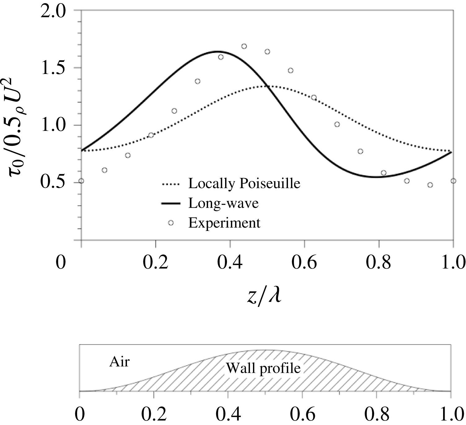
Once again we compare the model predictions for the wall stress with experiments. Two sinusoidally varying pipes were used in Hsu & Kennedy (Reference Hsu and Kennedy1971) with different amplitudes, and air was forced to flow at two different Reynolds numbers. Figure 8 shows a comparison of the model with two of the parameter settings from Hsu & Kennedy (Reference Hsu and Kennedy1971) with mean tube radius
 $0.204$
ft, wall wavelength
 $1.667$
ft and wall wave amplitude
 $0.0184$
ft (crest-to-trough amplitude
 $0.0368$
ft). The amplitude of the stress corrections seen in experiments is matched well by the first-order model, though the model overstates the phase shift by a considerable amount. The reasons why the model is able to more accurately capture the behaviour of wavy channel flow experiments in § 3 than those in pipes such as the ones here are not immediately clear, but there are several possible explanations. For example, both the Reynolds number and wave amplitude of the wavy pipe flow experiments are substantially higher than those of the channel flow experiments. In addition, the first-order model was derived while neglecting variations in the local Reynolds number due to the wall waviness. It is also possible that use of a different empirical formula other than (B 3)–(B 4) for the mixing length ratio may result in improved agreement between model and experiment. Nevertheless, the model appears to be an improvement over the LP model in all cases, and it will be incorporated into the liquid model next.
Comparison of locally Poiseuille (dashed line) and first-order (solid line) model predictions of wall shear stress for flow through a wavy pipe with experiments in Hsu & Kennedy (Reference Hsu and Kennedy1971) (circles).
 $Re_{P}^{(g)}=90\,000$
,
 $\bar{a}=0.204$
ft, wall wavelength is
 $1.667$
ft and wall wave amplitude is
 $0.0184$
ft (crest-to-trough amplitude
 $0.0368$
ft); the ratio of amplitude to wavelength has been enlarged in the wavy wall shown in the bottom panel.

In closing this section, we remark that the nonlinear response in the stress is visible in the model estimates in figure 8. The dependence on the axial coordinate of the wall shear stress is not given by a simple sinusoid; the distance when moving upstream from a crest to a trough in the wall shear stress is smaller than the distance moving upstream from a trough to a crest, while the wavy wall is sinusoidally varying.
5 Liquid modelling
Having found an estimate for the stresses exerted by the airflow on the free surface, we now return to the liquid flow along the interior of a vertical tube and derive a model for the evolution of the free surface utilizing long-wave asymptotics. We note that the no-slip boundary conditions used in the previous section for the airflow are justified by the large ratio of liquid and air viscosities, i.e.
 $\unicode[STIX]{x1D707}^{(l)}/\unicode[STIX]{x1D707}^{(g)}\gg 1$
.
5.1 Governing equations
The governing equations for the flow of the liquid film inside a vertical tube are the axisymmetric Navier–Stokes equations in cylindrical coordinates (2.1), made dimensionless here using the scalings
 $$\begin{eqnarray}\displaystyle \left.\begin{array}{@{}rcl@{}}r\ & =\ & \bar{r}/\bar{h}_{0},\quad z=\bar{z}/\bar{\unicode[STIX]{x1D706}},\quad \,u=\bar{u}/\bar{U}_{0},\\ w\ & =\ & \bar{w}/\bar{W}_{0},\quad t=\bar{t}\bar{W}_{0}/\bar{\unicode[STIX]{x1D706}},\quad p=\bar{p}\bar{h}_{0}/(\unicode[STIX]{x1D707}^{(l)}\bar{W}_{0}),\end{array}\right\} & & \displaystyle\end{eqnarray}$$
where
 $\bar{h}_{0}$
is the film’s mean thickness,
 $\bar{W}_{0}=g\unicode[STIX]{x1D70C}^{(l)}\bar{h}_{0}^{2}/\unicode[STIX]{x1D707}^{(l)}$
is the axial velocity scale,
 $\bar{U}_{0}=\unicode[STIX]{x1D716}\bar{W}_{0}$
is the radial velocity scale as determined by the continuity equation and
 $\unicode[STIX]{x1D716}=\bar{h}_{0}/\bar{\unicode[STIX]{x1D706}}\ll 1$
is the traditional long-wave aspect ratio small parameter. Substitution of (5.1) into (2.1) for the liquid flow yields
 $$\begin{eqnarray}\displaystyle \unicode[STIX]{x1D716}^{2}Re^{(l)}(u_{t}+uu_{r}+wu_{z}) & = & \displaystyle -p_{r}+\unicode[STIX]{x1D716}\left(\frac{1}{r}\unicode[STIX]{x2202}_{r}(ru_{r})+\unicode[STIX]{x1D716}^{2}u_{zz}-\frac{u}{r^{2}}\right),\end{eqnarray}$$
 $$\begin{eqnarray}\displaystyle \unicode[STIX]{x1D716}Re^{(l)}(w_{t}+uw_{r}+ww_{z}) & = & \displaystyle -\unicode[STIX]{x1D716}p_{z}+\frac{1}{r}\unicode[STIX]{x2202}_{r}(rw_{r})+\unicode[STIX]{x1D716}^{2}w_{zz}-1,\end{eqnarray}$$
 $$\begin{eqnarray}\displaystyle \frac{1}{r}\unicode[STIX]{x2202}_{r}(ru)+w_{z} & = & \displaystyle 0,\end{eqnarray}$$
 $\mathit{Re}^{(l)}\equiv \bar{\unicode[STIX]{x1D70C}}^{(l)}\bar{W}_{0}\bar{h}_{0}/\bar{\unicode[STIX]{x1D707}}^{(l)}$
is the liquid Reynolds number. The coordinate system is again oriented so that
 $\bar{z}$
increases moving up the tube.
Boundary conditions at the wall,
 $r=a$
, are no slip,
 $$\begin{eqnarray}\displaystyle u=w=0, & & \displaystyle\end{eqnarray}$$
and at the free surface,
 $r=R(z,t)$
, are
 $$\begin{eqnarray}\displaystyle w_{r}+O(\unicode[STIX]{x1D716}^{2}) & = & \displaystyle \unicode[STIX]{x1D70F}^{(g)},\end{eqnarray}$$
 $$\begin{eqnarray}\displaystyle -\!p+O(\unicode[STIX]{x1D716}) & = & \displaystyle -p^{(g)}+\frac{1}{Bo}\left(\frac{1}{R}-\unicode[STIX]{x1D716}^{2}R_{zz}\right),\end{eqnarray}$$
 $$\begin{eqnarray}\displaystyle w & = & \displaystyle R_{t}+uR_{z},\end{eqnarray}$$
 $$\begin{eqnarray}\displaystyle \unicode[STIX]{x1D70F}^{(g)}=\bar{\unicode[STIX]{x1D70F}}_{P}^{(g)}\bar{h}_{0}/(\unicode[STIX]{x1D707}^{(l)}\bar{W}_{0}),\quad p^{(g)}=\bar{P}_{P}^{(g)}\bar{h}_{0}/(\unicode[STIX]{x1D707}^{(l)}\bar{W}_{0}), & & \displaystyle\end{eqnarray}$$
and
 $$\begin{eqnarray}\displaystyle Bo & = & \displaystyle \bar{W}_{0}\unicode[STIX]{x1D707}^{(l)}/\unicode[STIX]{x1D6FE},\nonumber\\ \displaystyle & = & \displaystyle \frac{\unicode[STIX]{x1D70C}^{(l)}g\bar{a}^{2}}{\unicode[STIX]{x1D6FE}}\frac{1}{a^{2}},\end{eqnarray}$$
is the Bond number, where
 $\unicode[STIX]{x1D6FE}$
is surface tension. We note that a term of
 $O(\unicode[STIX]{x1D716}^{2})$
has been retained in (5.4b
) despite being formally of higher order; this term is traditionally kept in long-wave modelling to account for uniform matched-asymptotics validity (see, e.g. Oron, Davis & Bankoff (Reference Oron, Davis and Bankoff1997), and Craster & Matar (Reference Craster and Matar2009), for discussion of this term in models for related problems). Integrating the continuity equation across the annular-sectional area of the liquid and substituting (5.4c
) yields the layer-mean evolution equation
 $$\begin{eqnarray}\displaystyle R_{t}-\frac{1}{R}\frac{\unicode[STIX]{x2202}}{\unicode[STIX]{x2202}z}\int _{R}^{a}wr\,\text{d}r=0, & & \displaystyle\end{eqnarray}$$
for the location
 $R(z,t)$
of the free surface. All that is needed to close the model equation (5.7) is an estimate of the axial velocity
 $w$
.
5.2 Leading-order solution
The flow variables
 $u,w,p$
and stresses
 $p^{(g)}$
and
 $\unicode[STIX]{x1D70F}^{(g)}$
may be expanded in terms of the small parameter
 $\unicode[STIX]{x1D716}$
as
 $$\begin{eqnarray}\displaystyle u & = & \displaystyle u_{0}+\unicode[STIX]{x1D716}u_{1}+O(\unicode[STIX]{x1D716}^{2}),\end{eqnarray}$$
 $$\begin{eqnarray}\displaystyle w & = & \displaystyle w_{0}+\unicode[STIX]{x1D716}w_{1}+O(\unicode[STIX]{x1D716}^{2}),\end{eqnarray}$$
 $$\begin{eqnarray}\displaystyle p & = & \displaystyle p_{0}+\unicode[STIX]{x1D716}p_{1}+O(\unicode[STIX]{x1D716}^{2}),\end{eqnarray}$$
 $$\begin{eqnarray}\displaystyle p^{(g)} & = & \displaystyle p_{0}^{(g)}+\unicode[STIX]{x1D716}p_{1}^{(g)}+O(\unicode[STIX]{x1D716}^{2}),\end{eqnarray}$$
 $$\begin{eqnarray}\displaystyle \unicode[STIX]{x1D70F}^{(g)} & = & \displaystyle \unicode[STIX]{x1D70F}_{0}^{(g)}+\unicode[STIX]{x1D716}\unicode[STIX]{x1D70F}_{1}^{(g)}+O(\unicode[STIX]{x1D716}^{2}).\end{eqnarray}$$
 $O(1)$
are collected, the leading-order equations are given by
 $$\begin{eqnarray}\displaystyle \unicode[STIX]{x2202}_{r}p_{0}=0,\quad \frac{1}{r}\unicode[STIX]{x2202}_{r}(r\unicode[STIX]{x2202}_{r}w_{0})=1,\quad \unicode[STIX]{x2202}_{r}(ru_{0})=-r\unicode[STIX]{x2202}_{z}w_{0}, & & \displaystyle\end{eqnarray}$$
with leading-order boundary conditions at the wall
 $r=a$
given by
 $$\begin{eqnarray}\displaystyle u_{0}=w_{0}=0, & & \displaystyle\end{eqnarray}$$
and at the free surface
 $r=R(z,t)$
by
 $$\begin{eqnarray}\displaystyle \unicode[STIX]{x2202}_{r}w_{0} & = & \displaystyle \unicode[STIX]{x1D70F}_{0}^{(g)},\quad p_{0}=p_{0}^{(g)}.\end{eqnarray}$$
The leading-order stress
 $\unicode[STIX]{x1D70F}_{0}^{(g)}$
imparted by the gas flow at the interface can be approximated using
 $\bar{\unicode[STIX]{x1D70F}}_{P_{0}}^{(g)}$
found in (4.14), here non-dimensionalized by the liquid scalings,
 $$\begin{eqnarray}\displaystyle \unicode[STIX]{x1D70F}_{0}^{(g)} & = & \displaystyle -\frac{\tilde{T}_{w0}a^{3}(a-1)}{R^{3}},\end{eqnarray}$$
where
 $$\begin{eqnarray}\displaystyle \tilde{T}_{w0} & = & \displaystyle \frac{|\bar{T}_{P}|(a-1)^{3}}{\unicode[STIX]{x1D70C}^{(l)}g\bar{h}_{0}a^{3}}=\frac{0.079(\unicode[STIX]{x1D707}^{(g)})^{2}}{8g\unicode[STIX]{x1D70C}^{(g)}\unicode[STIX]{x1D70C}^{(l)}\bar{a}^{3}}(Re_{P}^{(g)})^{7/4},\end{eqnarray}$$
while the leading-order pressure gradient can be approximated by
 $$\begin{eqnarray}\displaystyle p_{0z}^{(g)}=\frac{2\unicode[STIX]{x1D70F}_{0}^{(g)}}{R} & = & \displaystyle -\frac{2\tilde{T}_{w0}a^{3}(a-1)}{R^{4}}.\end{eqnarray}$$
Substituting (5.12) into (5.11) and solving (5.9)–(5.11) results in the leading-order velocity profile
 $$\begin{eqnarray}\displaystyle w_{0} & = & \displaystyle \frac{1}{4}\left[r^{2}-a^{2}-2\left(R^{2}+\frac{2\tilde{T}_{w0}a^{3}(a-1)}{R^{2}}\right)\log \frac{r}{a}\right],\end{eqnarray}$$
 $$\begin{eqnarray}\displaystyle u_{0} & = & \displaystyle \frac{1}{4r}\left(a^{2}-r^{2}+2r^{2}\log \frac{r}{a}\right)\left[R-\frac{2\tilde{T}_{w0}a^{3}(a-1)}{R^{3}}\right]R_{z}.\end{eqnarray}$$
5.3 First-order corrections
Collecting all terms of
 $O(\unicode[STIX]{x1D716})$
in (5.2b
) results in
 $$\begin{eqnarray}\displaystyle \unicode[STIX]{x2202}_{r}p_{1} & = & \displaystyle \frac{1}{r}\unicode[STIX]{x2202}_{r}(r\unicode[STIX]{x2202}_{r}u_{0})-\frac{u_{0}}{r^{2}},\end{eqnarray}$$
 $$\begin{eqnarray}\displaystyle \frac{1}{r}\unicode[STIX]{x2202}_{r}(r\unicode[STIX]{x2202}_{r}w_{1}) & = & \displaystyle \mathit{Re}^{(l)}(\unicode[STIX]{x2202}_{t}w_{0}+u_{0}\unicode[STIX]{x2202}_{r}w_{0}+w_{0}\unicode[STIX]{x2202}_{z}w_{0})+\unicode[STIX]{x2202}_{z}p_{0},\end{eqnarray}$$
 $$\begin{eqnarray}\displaystyle \frac{1}{r}\unicode[STIX]{x2202}_{r}(ru_{1})+\unicode[STIX]{x2202}_{z}w_{1} & = & \displaystyle 0.\end{eqnarray}$$
 $Re^{(l)}=O(\unicode[STIX]{x1D716})$
; this is consistent with the experiments in Camassa et al. (Reference Camassa, Forest, Lee, Ogrosky and Olander2012) for which the liquid Reynolds number was estimated to be
 $Re^{(l)}=O(10^{-2})$
. Under this assumption our equation (5.16b
) for
 $w_{1}$
reduces to
 $$\begin{eqnarray}\displaystyle \frac{1}{r}\unicode[STIX]{x2202}_{r}(r\unicode[STIX]{x2202}_{r}w_{1})=\unicode[STIX]{x2202}_{z}p_{0}. & & \displaystyle\end{eqnarray}$$
At
 $O(\unicode[STIX]{x1D716})$
, the boundary conditions at the wall (
 $r=a$
) are
 $$\begin{eqnarray}\displaystyle u_{1}=w_{1}=0, & & \displaystyle\end{eqnarray}$$
and at the free surface (
 $r=R(z,t)$
) are
 $$\begin{eqnarray}\displaystyle \unicode[STIX]{x2202}_{r}w_{1} & = & \displaystyle \unicode[STIX]{x1D70F}_{1}^{(g)},\quad p_{1}=p_{1}^{(g)}.\end{eqnarray}$$
The first-order shear stress corrections
 $\unicode[STIX]{x1D70F}_{1}^{(g)}$
can be approximated by
 $\bar{\unicode[STIX]{x1D70F}}_{P_{1}}^{(g)}$
in (B 7),
 $$\begin{eqnarray}\displaystyle \unicode[STIX]{x1D70F}_{1}^{(g)} & = & \displaystyle \frac{\tilde{T}_{w1}a^{3}(a-1)^{2}}{R^{4}}R_{z},\end{eqnarray}$$
where
 $$\begin{eqnarray}\displaystyle \tilde{T}_{w1}=B_{P}^{\ast }\tilde{T}_{w0}, & & \displaystyle\end{eqnarray}$$
with
 $B_{P}^{\ast }$
defined in (B 8). Substituting (5.14) and (5.20) into (5.17) and (5.19), respectively, and solving (5.17)–(5.19) for
 $w_{1}$
results in
 $$\begin{eqnarray}\displaystyle w_{1} & = & \displaystyle \frac{1}{4}\left[-\frac{2\tilde{T}_{w0}a^{3}(a-1)}{R^{4}}R_{z}+\frac{1}{Bo}\left(\frac{R_{z}}{R^{2}}+\unicode[STIX]{x1D716}^{2}R_{zzz}\right)\right](r^{2}-a^{2})\nonumber\\ \displaystyle & & \displaystyle +\left[\frac{\tilde{T}_{w1}a^{3}(a-1)^{2}}{R^{3}}R_{z}+\frac{\tilde{T}_{w0}a^{3}(a-1)}{R^{2}}R_{z}-\frac{1}{Bo}(R_{z}+\unicode[STIX]{x1D716}^{2}R^{2}R_{zzz})\right]\log \frac{r}{a}.\qquad\end{eqnarray}$$
The first-order long-wave model then results from substitution of
 $w=w_{0}+w_{1}$
into (5.7). After adopting the convention of rescaling
 $z$
and
 $t$
by
 $\unicode[STIX]{x1D716}$
to return to the original aspect ratio, this model equation is
 $$\begin{eqnarray}\displaystyle & & \displaystyle R_{t}+\frac{1}{2}\left[\tilde{T}_{w0}a^{3}(a-1)f_{1}(R;a)-f_{2}(R;a)\right]R_{z}\nonumber\\ \displaystyle & & \displaystyle \quad +\,\frac{1}{16R}\left[16Sf_{3}(R;a)(R_{z}+R^{2}R_{zzz})+4\tilde{T}_{w1}a^{3}(a-1)^{2}f_{2}(R;a)R^{-3}R_{z}\right]_{z}=0,\qquad\end{eqnarray}$$
where
 $$\begin{eqnarray}\displaystyle f_{1}(R;a) & = & \displaystyle \frac{a^{2}}{R^{4}}\left(\frac{a^{2}}{R^{2}}-1\right),\end{eqnarray}$$
 $$\begin{eqnarray}\displaystyle f_{2}(R;a) & = & \displaystyle a^{2}-R^{2}+2R^{2}\log (R/a),\end{eqnarray}$$
 $$\begin{eqnarray}\displaystyle f_{3}(R;a) & = & \displaystyle \frac{a^{4}}{R^{2}}-4a^{2}+3R^{2}-4R^{2}\log (R/a),\end{eqnarray}$$
 $S=1/16Bo$
.
The LP model studied in Camassa et al. (Reference Camassa, Forest, Lee, Ogrosky and Olander2012) is recovered if we set
 $\tilde{T}_{w1}=0$
, given here for later reference,
 $$\begin{eqnarray}R_{t}+\frac{1}{2}\left[\tilde{T}_{w0}a^{3}(a-1)f_{1}(R;a)-f_{2}(R;a)\right]R_{z}+\frac{1}{16R}\left[16Sf_{3}(R;a)(R_{z}+R^{2}R_{zzz})\right]_{z}=0.\end{eqnarray}$$
In the case of no imposed airflow, i.e.
 $\tilde{T}_{w0}=\tilde{T}_{w1}=0$
, the model of Part 1 (Camassa et al.
Reference Camassa, Ogrosky and Olander2014) studied by Camassa et al. (Reference Camassa, Marzuola, Ogrosky and Vaughn2016) is recovered, and is similar in form to models for the flow of a film down the exterior of a tube (Lin & Liu Reference Lin and Liu1975; Kliakhandler, Davis & Bankoff Reference Kliakhandler, Davis and Bankoff2001; Craster & Matar Reference Craster and Matar2006).
The coefficients
 $\tilde{T}_{w0}$
and
 $\tilde{T}_{w1}$
are functions of the gas Reynolds number
 $Re_{P}^{(g)}$
(which itself depends on the film thickness parameter
 $a$
). Thus the model is seen to depend on three parameters: a film thickness parameter
 $a$
, the gas Reynolds number
 $Re_{P}^{(g)}$
and Bond number
 $Bo$
. In experiments conducted in Camassa et al. (Reference Camassa, Forest, Lee, Ogrosky and Olander2012) the Bond number was identical in each realization of the experiment, and we will likewise focus on the model’s behaviour for various values of
 $a$
and
 $Re_{P}^{(g)}$
, keeping
 $Bo$
fixed in § 6.
We remark that the model retains the cylindrical geometry of the problem, a feature which has been shown to be important for certain types of model behaviour in related models (Camassa & Ogrosky Reference Camassa and Ogrosky2015). Note also that the free-surface evolution according to the long-wave model depends only on the local tube radius and its gradients.
5.4 Thin-film limit
The long-wave model (5.23) was derived without assuming the film’s thickness was small relative to the tube. If the film is taken to be thin, i.e. let
 $\unicode[STIX]{x1D6FD}=1/a\ll 1$
, then (5.23) can be simplified by expanding each function
 $f_{i}$
in (5.24) in terms of
 $\unicode[STIX]{x1D6FD}$
,
 $$\begin{eqnarray}\displaystyle f_{1} & = & \displaystyle 2h\unicode[STIX]{x1D6FD}^{3}+O(\unicode[STIX]{x1D6FD}^{4}),\end{eqnarray}$$
 $$\begin{eqnarray}\displaystyle f_{2} & = & \displaystyle 2h^{2}+O(\unicode[STIX]{x1D6FD}),\end{eqnarray}$$
 $$\begin{eqnarray}\displaystyle f_{3} & = & \displaystyle \frac{16h^{3}}{3}\unicode[STIX]{x1D6FD}+O(\unicode[STIX]{x1D6FD}^{2}),\end{eqnarray}$$
 $$\begin{eqnarray}\displaystyle h=\frac{1}{\unicode[STIX]{x1D6FD}}-R & & \displaystyle\end{eqnarray}$$
represents the thickness of the annular film. Substitution of (5.27) and (5.26) into (5.23) results in
 $$\begin{eqnarray}\displaystyle h_{t}+(\tilde{T}_{w0}h-\unicode[STIX]{x1D6FD}h^{2})h_{z}+\left[\frac{16\unicode[STIX]{x1D6FD}\tilde{S}}{3}h^{3}\left(h_{z}+\frac{h_{zzz}}{\unicode[STIX]{x1D6FD}^{2}}\right)+\frac{\tilde{T}_{w1}}{2}h^{2}h_{z}\right]_{z}=0, & & \displaystyle\end{eqnarray}$$
where
 $\tilde{S}=\unicode[STIX]{x1D6FD}^{2}S$
.
This thin-film limit ‘flattens’ the geometry by neglecting the local azimuthal curvature of the surface over scales of the film thickness. It is perhaps not surprising then that the
 $\tilde{T}_{w1}$
term in (5.28) is of a somewhat similar form to the corresponding term in the flat-film long-wave model in Tseluiko & Kalliadasis (Reference Tseluiko and Kalliadasis2011) (their equation (4.62)), with the important distinction that here the correction is specified by
 $h$
and its axial derivatives rather than global information through the Fourier modes of
 $h$
. These models are of course also distinct from one another in the destabilizing role played by capillary forces due to the azimuthal curvature in the cylindrical set-up considered here.
We note that several related thin-film models can be recovered from (5.28) under appropriate limits. If only the leading-order effects of the airflow are included (i.e. set
 $\tilde{T}_{w1}$
to zero) and the effects of gravity are considered negligible (i.e. the term
 $\unicode[STIX]{x1D6FD}h^{2}h_{z}$
in (5.28) is neglected), the model derived and studied by Kerchman (Reference Kerchman1995) is recovered. If, instead, there is no imposed airflow (i.e.
 $\tilde{T}_{w0}=\tilde{T}_{w1}=0$
), the model derived by Frenkel (Reference Frenkel1992) and studied by Kalliadasis & Chang (Reference Kalliadasis and Chang1994) and Kerchman & Frenkel (Reference Kerchman and Frenkel1994) is recovered. Finally, if both gravity and the effects of airflow are considered negligible, the model derived by Hammond (Reference Hammond1983) and studied by Lister et al. (Reference Lister2006) is recovered.
6 Results
Solutions to the first-order long-wave model equation (5.23) are next studied analytically and numerically, and compared with solutions to the LP model (5.25).
(a,c) Dimensionless wavenumber of maximum growth rate,
 $k_{m}$
, for the (a) long-wave model and (c) locally Poiseuille model for film flow inside a vertical tube. (b,d) Dimensional wavelength of maximum growth rate,
 $\bar{\unicode[STIX]{x1D706}}_{m}$
, for the (b) long-wave model and (d) locally Poiseuille model. Curves of constant volume flux of air are shown for
 $\bar{Q}_{P}=330$
,670 and
 $1000~\text{cm}^{3}~\text{s}^{-1}$
with all other parameters matching those of the experiments in Camassa et al. (Reference Camassa, Forest, Lee, Ogrosky and Olander2012).

6.1 Linear stability analysis
We first study the long-wave model (5.23) by introducing an infinitesimal perturbation to the free surface,
 $$\begin{eqnarray}\displaystyle R=(a-1)+A\exp [\text{i}(kz-\unicode[STIX]{x1D714}t)], & & \displaystyle\end{eqnarray}$$
where
 $A\ll a-1$
is the amplitude of the disturbance,
 $k$
is its real wavenumber,
 $\text{Re}[\unicode[STIX]{x1D714}]/k$
is its phase speed and
 $\unicode[STIX]{x1D706}=\text{Im}[\unicode[STIX]{x1D714}]$
is its growth rate. Substituting (6.1) into (5.23) and neglecting higher-order terms in
 $A$
gives the dispersion relation
 $$\begin{eqnarray}\displaystyle \unicode[STIX]{x1D714}_{LW} & = & \displaystyle \frac{1}{2}\left[\tilde{T}_{w0}a^{3}(a-1)f_{1}(a-1;a)-f_{2}(a-1;a)\right]k\nonumber\\ \displaystyle & & \displaystyle +\,\frac{i}{16(a-1)}\!\left[16Sf_{3}(a-1;a)[k^{2}-(a-1)^{2}k^{4}]+\frac{4\tilde{T}_{w1}a^{3}f_{2}(a-1;a)}{a-1}k^{2}\right]\!.\quad\end{eqnarray}$$
The dispersion relation for the locally Poiseuille model is again recovered by setting
 $\tilde{T}_{w1}=0$
, i.e.
 $$\begin{eqnarray}\displaystyle \unicode[STIX]{x1D714}_{LP} & = & \displaystyle \frac{1}{2}\left[\tilde{T}_{w0}a^{3}(a-1)f_{1}(a-1;a)-f_{2}(a-1;a)\right]k\nonumber\\ \displaystyle & & \displaystyle +\frac{i}{16(a-1)}\left[16Sf_{3}(a-1;a)[k^{2}-(a-1)^{2}k^{4}]\right].\end{eqnarray}$$
As the real components of (6.2) and (6.3) are identical, the speed of infinitesimal free-surface disturbances in both models is the same.
In the long-wave model, the free-surface stress created by the airflow contributes to both the real and imaginary components of the dispersion relation. The imaginary component contributes to instability growth and plays a role in determining the wavelength of maximum growth rate,
 $$\begin{eqnarray}\displaystyle k_{m,LW} & = & \displaystyle \frac{1}{\sqrt{2}(a-1)}\left[1+\frac{4\tilde{T}_{w1}a^{3}f_{2}(a-1;a)}{16S(a-1)f_{3}(a-1;a)}\right]^{1/2}.\end{eqnarray}$$
From (6.4) it can be seen that increasing
 $\tilde{T}_{w1}$
results in increasing
 $k_{m,LW}$
, so that higher airflow rates result in shorter free-surface waves. In contrast, in the locally Poiseuille model the airflow only contributes to the real part of the dispersion relation and does not contribute to instability growth. The wavelength of maximum growth rate for the locally Poiseuille model is
 $$\begin{eqnarray}\displaystyle k_{m,LP}=\frac{1}{\sqrt{2}(a-1)}; & & \displaystyle\end{eqnarray}$$
note that this growth rate is identical to the growth rate for the gravity-driven model in Part 1 (Camassa et al. Reference Camassa, Ogrosky and Olander2014).
Dimensionless growth rates
 $\unicode[STIX]{x1D714}(k_{m})$
for (a) long-wave model and (b) locally Poiseuille model for film flow inside a vertical tube. Curves denote constant volume flux of air (see caption for figure 9).

The wavenumber
 $k_{m}$
of maximum growth rate for each model is shown in figure 9 for various film thicknesses (as measured by
 $\unicode[STIX]{x1D6FD}=1/a$
) and gas Reynolds numbers
 $Re_{P}^{(g)}$
. In the locally Poiseuille model (lower panels), the wavenumber of maximum growth rate is solely determined by film thickness, while the wavelength depends on both film thickness and gas Reynolds number in the long-wave model. Note that for a given Reynolds number, there is a film thickness which results in a wavelength of maximum growth rate which is longer than for any other film thickness.
The growth rate for each model is shown in figure 10. For the locally Poiseuille model, the growth rate is again independent of Reynolds number, while the growth rate for the long-wave model increases with increasing film thickness and increasing Reynolds number.
In the experiments conducted in Camassa et al. (Reference Camassa, Forest, Lee, Ogrosky and Olander2012), the volume flux of gas was prescribed; the Reynolds number
 $Re_{P}^{(g)}$
depends on both the volume flux and film thickness. Curves of constant volume flux corresponding to some values from these experiments are overlaid onto figures 9 and 10 for reference.
6.2 Comparison with experiment
We next turn to a brief investigation of how well these linear stability analysis results match experiments. A direct comparison with Camassa et al. (Reference Camassa, Forest, Lee, Ogrosky and Olander2012) would be ideal. However, in these experiments most of the waves observed enter the test section already developed as large-amplitude ring waves. Thus the waves appear to already be well outside the linear regime when they are first visible in the tube. Furthermore, these waves travel the length of the tube with such frequency and speed that they overcome the long-wave instability before it has time to grow into a visible wave.
In order to produce waves that are suitable for comparing with the model results above, a modified version of one of the experiments in Camassa et al. (Reference Camassa, Forest, Lee, Ogrosky and Olander2012) was performed. The basic set-up of the experiment remained the same: a 20.0 cm glass tube with a 1.0 cm inner diameter was inserted into an O-ring-lined hole in the lid of an annular chamber made of stainless steel and glass. A viscous silicone oil was forced into the annulus of the chamber at a constant volume flux by a Harvard Apparatus Model 975 Syringe Pump and was allowed to fill the chamber up to a small annular gap of 1 mm. A constant volume flux of air was forced through the core of the chamber by an Aalborg Digital Flow Controller where it met the liquid at the gap. The oil’s viscosity was 129 P and its density was
 $0.97~\text{g}~\text{cm}^{-3}$
; the volume flux of air was
 $330~\text{cm}^{3}~\text{s}^{-1}$
. The experiment was filmed in high definition with a Sony Handycam HDR-FX1.
Once the tube was completely coated, the flow of oil into the bottom of the tube was stopped. In the several minutes immediately following this oil shutoff, the airflow continued to drive the oil upwards out the top of the tube into a collection cup. With no replenishing supply of oil at the bottom of the tube, the oil film’s thickness decreased slightly during this time. The film eventually settled into a quasi-steady regime, where downward movement of fluid due to gravity was balanced by upward movement due to the free-surface stress imparted by the airflow. After reaching this quasi-steady state, large-amplitude waves were no longer generated at the inlet. This allowed the long-wave instabilities sufficient time to develop at the free surface and quickly saturate into large-amplitude waves.
Measured wavelengths in ‘zero-oil-feed’ experiment;
 $\bar{Q}=330~\text{cm}^{3}~\text{s}^{-1}$
,
 $\unicode[STIX]{x1D707}^{(l)}=129$
P,
 $\unicode[STIX]{x1D70C}^{(l)}=0.97~\text{g}~\text{cm}^{-3}$
,
 $\bar{a}=0.5~\text{cm}$
and
 $\bar{h}_{0}\approx 0.094~\text{cm}$
. Time is measured in seconds after the oil feed was shut off.

The wavelengths of these free-surface perturbations were measured from the recorded video of the experiment, and then they were compared with the wavelength of maximum growth rate from the model. Regarding the experimental measurements, it should be noted that the low-amplitude disturbances that are observed are likely already beginning to saturate into nonlinear waves. However, with the aid of a checkered background the otherwise invisible distortions can be seen and their wavelength measured and then compared with the model. Figure 11 shows the wavelengths observed in this experiment with a line of best fit. While there is some slope to the line of best least-square fit and significant variability in the wavelengths is observed, it appears that for most of the duration of the experiment, a typical wavelength may be taken to be approximately 1 cm. (The few outliers are likely a consequence of the difficulty in distinguishing some of these very low-amplitude waves.) The mean thickness of the film (determined by the weight method described in Part 1) in these experiments was measured to be approximately 0.094 cm, so that
 $\unicode[STIX]{x1D6FD}\approx 0.19$
. The wavelength of maximum growth rate for the long-wave model is thus approximately 1.8 cm, which may be found from (6.2) or figure 9; for the locally Poiseuille model, the wavelength of maximum growth rate is approximately 3.6 cm. Thus both models overestimate the most unstable wavelength, but the long-wave model represents a significant improvement over the locally Poiseuille model. However, it must be stressed that the measurement of wavelength in the experiment is only possible for waves that have evolved to be visually detectable in the pipe, and this could be already somewhat far from a purely linear regime. As shown below in numerical simulations of the long-wave model, small and shorter waves appear, at approximately half the most unstable wavelength, before fully nonlinear waves develop and dominate the dynamics. Since measuring wavelengths in the experiment was only possible for waves that had grown to amplitudes that could be readily discerned by eye, and as a result, many of these waves may have already been affected by nonlinearity, we turn to approximate nonlinear model solutions to explore these regimes.
6.3 Nonlinear results
The saturation of the free-surface instabilities discussed above is now examined. The experiments reported in Camassa et al. (Reference Camassa, Forest, Lee, Ogrosky and Olander2012) showed that the locally Poiseuille model is not able to adequately capture the transfer of momentum from the airflow to the annular film. For example, for a given set of parameter values, the locally Poiseuille model was unable to capture the velocity of saturated free-surface disturbances; for a wide range of parameter values, the model exhibited saturated instabilities propagating down the tube while in the experiment the observed saturated waves travelled up the tube. One ad hoc remedy for this discrepancy is to simply replace the viscosity with a modified viscosity; an estimate of this modified viscosity was made based on the ratio of air and liquid viscosities in Camassa & Lee (Reference Camassa, Lee, Chwang, Teng and Valentine2006) and Camassa et al. (Reference Camassa, Forest, Lee, Ogrosky and Olander2012). This remedy was shown to dramatically reduce the discrepancy in wave speed between experiments and model, but this improvement came at the expense of realistic wave profiles. Specifically, model solutions found with the modified viscosity exhibited very small-amplitude waves, while the experiments indicated that the waves can saturate with large amplitude. We next explore whether the long-wave model derived here is able to produce large-amplitude waves with higher upwards speed without resorting to an empirically modified viscosity.
(a) Time snapshots showing the evolution of solutions to the long-wave model (5.23) for film flow inside a vertical tube in a periodic domain for
 $\bar{a}=0.5~\text{cm}$
,
 $\bar{R}_{0}=0.25~\text{cm}$
,
 $\bar{Q}=330~\text{cm}^{3}~\text{s}^{-1}$
,
 $\unicode[STIX]{x1D707}^{(l)}=600$
P. Interfacial profiles are shown successively shifted at equal time intervals. Profiles are shown in the laboratory frame of reference. Gravity acts from right to left. (b) Time snapshots of solutions to the locally Poiseuille model (5.25) for the same parameter values as (a).

Solutions to both models with periodic boundary conditions are found numerically by the method of lines using a pseudospectral algorithm calculating spatial derivatives in Fourier space and nonlinear terms in physical space. The free surface is evolved in time using a simple second-order predictor–corrector integration scheme. The Fourier modes of the derivatives and various nonlinear terms are monitored throughout the simulation to check conservation of volume. The initial conditions used for all simulations here are a flat free surface superposed with small-amplitude disturbances of several wavenumbers; the long-time behaviour of the interface does not appear to be sensitive to the exact choice of wavenumbers and amplitudes. See Camassa et al. (Reference Camassa, Forest, Lee, Ogrosky and Olander2012) for more details of the numerical procedure.
Figure 12 shows the evolution of the free surface in the long-wave model (5.23) and the locally Poiseuille model (5.25). Here each panel is oriented so that gravity acts from right to left. Successive snapshots of the free surface are shown at equally spaced time intervals, with time increasing moving up the vertical axis; snapshots are shown in a laboratory reference frame. The scale for the amplitude of the free-surface disturbances is given at the top left for the final profile.
For both the long-wave and locally Poiseuille models, the instabilities initially move down the tube as the effects of gravity are stronger than the free-surface stresses caused by the core flow. In this initial period of time the waves are in a linear regime, and the velocity of the waves in each model are approximately identical as expected. This initial time period of linear growth is shorter for the long-wave model, consistent with the higher growth rates found in the linear stability analysis of this model. We note that in the long-wave model solution from approximately
 $t=40$
s to
 $t=60$
s, the waves have not yet saturated, but are beginning to shorten; i.e. the number of wave crests in the domain is larger than that predicted by linear stability analysis. Thus the model’s wavelength estimate of 1.8 cm provided by linear stability analysis is likely an overestimate when comparing with observed waves in the experiment.
At approximately
 $t=60$
s, free-surface disturbances in the long-wave model begin to saturate as large-amplitude waves; the nonlinear balance struck in these steady waves results in propagation up the tube. These waves undergo a brief period of acceleration as they propagate over smaller disturbances, but otherwise maintain their speed and shape. Disturbances to the locally Poiseuille model also grow into a steady wave train, but the amplitude of these waves is much smaller than those of the long-wave model. These waves continue to propagate down the tube, with speed diminished only slightly by the nonlinearities in the free-surface stresses caused by the core flow.
(a) Maximum value of
 $h-h_{0}$
as a function of
 $t$
for the long-wave (dashed) and locally Poiseuille (solid) models for film flow inside a vertical tube. (b) Location
 $z_{max}$
of the maximum value at each time. Light dashed-dotted lines indicate the linear theory; light dotted lines denote the amplitude and speed of the travelling wave solutions in figure 14.

The simulation was run again with a domain size determined by a single wavelength
 $\unicode[STIX]{x1D706}_{m}$
of maximum growth rate. Figure 13 compares the amplitude (mean to crest) of the wave and the location
 $z$
of the wave with the linear theory for each model. For times
 $t<14$
s, the growth and propagation of the instability in both models are in excellent agreement with the linear theory. For
 $t>17$
s, the instability in the long-wave model has saturated and propagates up the tube. The locally Poiseuille model is in good agreement with the linear theory until
 $t\approx 100$
s, when it saturates at much smaller amplitude, continuing down the tube with reduced speed.
These numerical simulations indicate that in both the long-wave (5.23) and locally Poiseuille (5.25) models the perturbed interface eventually settles into a series of travelling waves. Travelling wave solutions can be found by switching to a frame of reference moving with the wave, i.e.
 $$\begin{eqnarray}\displaystyle Z=z-ct, & & \displaystyle\end{eqnarray}$$
where
 $c$
is the speed of the wave. Substitution of (6.6) into the long-wave model yields a fourth-order ordinary differential equation (ODE)
 $$\begin{eqnarray}\displaystyle cR^{\prime } & = & \displaystyle \frac{1}{2}\left[\tilde{T}_{w0}a^{3}(a-1)f_{1}(R;a)-f_{2}(R;a)\right]R^{\prime }\nonumber\\ \displaystyle & & \displaystyle +\,\frac{1}{16R}\frac{\text{d}}{\text{d}Z}\left[16Sf_{3}(R;a)(R^{\prime }+R^{2}R^{\prime \prime \prime })+4\tilde{T}_{w1}a^{3}(a-1)^{2}f_{2}(R;a)R^{-3}R^{\prime }\right].\end{eqnarray}$$
Travelling wave solutions for the locally Poiseuille model can be found by solving (6.7) with
 $\tilde{T}_{w1}=0$
; such solutions were found numerically in Camassa et al. (Reference Camassa, Forest, Lee, Ogrosky and Olander2012). The same procedure, where an initial guess taken from a long-time simulation of each PDE is provided to an iteration scheme for solving boundary value problems, is used here to find solutions for the long-wave case where
 $\tilde{T}_{w1}$
is defined by (5.21).
Travelling wave solutions for the long-wave (dashed) and locally Poiseuille (solid) models for film flow inside a vertical tube.

Figure 14 shows the profile of travelling wave solutions from each model for the same parameter settings as in figures 12 and 13. Consistent with the long-time behaviour seen in figures 12 and 13, the amplitude of the solution to the long-wave model is significantly larger and has smaller wavelength than that of the locally Poiseuille model. These differences persist across various parameter values; figure 14 shows solutions with airflow rate large enough to result in upwards motion of the waves in both models. The waves in the locally Poiseuille model are very close to reversing direction, or ‘flooding’, and yet show significantly smaller amplitude than the long-wave model. We note that streamlines of the annular fluid flow may also be found for each model’s travelling wave solution. In Camassa et al. (Reference Camassa, Forest, Lee, Ogrosky and Olander2012) it was shown that some of the locally Poiseuille travelling wave solutions have a region of recirculating fluid, or a trapped core, near the wave crest. Similarly, trapped cores exist in some of the long-wave solutions; these cores lie near the wave crest, but are shifted somewhat so that their centre does not lie at the same
 $Z$
location as the wave crest (not shown).
All of the results presented here indicate that the long-wave model captures the stresses exerted by the airflow on the free surface better than the locally Poiseuille model. However, the long-wave model still appears unable to fully capture the exchange of momentum between air and liquid seen in experiments. For example, in addition to underestimating the speed of saturated disturbances, the locally Poiseuille model was also shown to grossly underestimate the volume flux of the annular film for a given film thickness and airflow rate in the experiments of Camassa et al. (Reference Camassa, Forest, Lee, Ogrosky and Olander2012). A brief investigation into the long-wave model indicates that it offers only a slight improvement over the locally Poiseuille model in estimating volume flux as a function of film thickness.
It is however important to note again that making a direct comparison between the long-wave model and the experiments of Camassa et al. (Reference Camassa, Forest, Lee, Ogrosky and Olander2012) is further complicated by the experimental set-up. In those experiments, many of the waves observed in the annular film were generated at the inlet where the oil was fed into the test section, and not within the test section. These inlet-generated waves are not being modelled here, and while it is possible that some of their features such as amplitude, profile and propagation may be well described by asymptotic models, it is by no means clear that they need be. One might hope to make a comparison between the speed of the saturated model waves with the speed of large-amplitude waves observed in the experiments reported in § 6.2, since many of the large-amplitude waves were observed to grow in the test section rather than be generated at the inlet. These waves, however, exhibit a ‘stop-and-go’-type movement, where they remain either motionless or nearly motionless for several seconds, before quickly advancing by a small increment whenever they collide with another, smaller-amplitude wave that is moving slowly down the tube. We note that this behaviour is qualitatively seen in model simulations for identical parameters as those in the experiment (with the exception of a different film thickness,
 $\bar{h}_{0}=0.17~\text{cm}$
). Two movies that demonstrate this behaviour have been included in the online supplementary information that accompanies this article available at https://doi.org/10.1017/jfm.2017.409: one of a model simulation, and one of an experiment. In both movies, the tube radius is
 $\bar{a}=0.5~\text{cm}$
and the airflow rate is
 $\bar{Q}_{P}=330~\text{cm}^{3}~\text{s}^{-1}$
. In the experiment movie, the viscosity is
 $\unicode[STIX]{x1D707}^{(l)}=129$
P and the film thickness was measured to be approximately
 $\bar{h}=0.10~\text{cm}$
; in the simulation, the viscosity is
 $\unicode[STIX]{x1D707}^{(l)}=600$
P and the film thickness was
 $\bar{h}=0.17~\text{cm}$
. A thorough comparison of the model with experiments, however, is an area that requires further investigation, and is left for future work.
Before concluding, we briefly consider each of the approximations made in deriving the long-wave model and how applicable each one is to the experiments of Camassa et al. (Reference Camassa, Forest, Lee, Ogrosky and Olander2012). The assumption of a large ratio of velocity scales between air and liquid is likely satisfied in the experiments due to a large ratio of viscosities of the liquid and air (
 $\unicode[STIX]{x1D707}^{(l)}/\unicode[STIX]{x1D707}^{(g)}\approx 10^{6}$
). Photographic snapshots (not shown) of the fully saturated waves in the experiments indicate that the long-wave aspect ratio approximation is likely valid, though quantifying this ratio in the experiment is difficult given the challenges of measuring the exact location of the free surface due to refraction through the curved glass and liquid film. The results in figures 12 and 14 suggest that the saturated waves have a smaller base of support than the linear waves described by the dispersion relation (6.4); e.g. the saturated waves in figure 12 each have a base of support of approximately 1 cm. Meanwhile the various radial scales of the problem, i.e. the mean thickness of the film, tube radius and mean radius of gas core, lie between approximately 0.25 cm and 0.5 cm. Thus it is not clear that
 $\bar{L}_{R}/\bar{\unicode[STIX]{x1D706}}^{\ast }\ll 1$
throughout all simulations, where
 $\bar{L}_{R}$
is a radial length scale and
 $\bar{\unicode[STIX]{x1D706}}^{\ast }$
is a typical saturated wavelength. There are many other examples in the literature, however, of asymptotic models proving to be effective well outside their strict range of validity, including some cases where the small parameter is considerably greater than 1; in contrast, it appears that here
 $\bar{L}_{R}/\bar{\unicode[STIX]{x1D706}}^{\ast }<1$
, at least throughout all simulations shown here.
The issue of empirically estimating the leading-order wall stress in pipe flow has been investigated extensively, and while the approximation of the stress used here is simple, previous studies indicate it is likely reasonable. However, the degree to which other approximations are applicable to the experiments is difficult to assess. For example, the model derivation assumes that the wall perturbations are not of the same order of magnitude as the tube radius; in both the experiments and some of the model solutions, this ordering appears to break down. In addition, we have neglected the contribution of normal Reynolds stresses, and also required that all of the airflow’s volume flux occurs at the leading order, leaving the first-order corrections to make a net-zero contribution to the volume flux at every point in
 $(z,t)$
space; it is unclear whether these assumptions are applicable to the experiments. Any of these approximations could be a source of the discrepancy between momentum exchange in the model and in the experiment. Despite these ongoing challenges, the results shown here indicate that this new long-wave model is able to create more realistic free-surface disturbances than its predecessors.
7 Conclusions
We have derived a new model for the flow of a liquid film coating the interior of a vertical rigid tube in the presence of upwards pressure-driven airflow. The model was derived by decoupling the airflow from the coupled problem and estimating the stresses the airflow exerts on a rigid wavy wall; these estimates were derived for both the case of wavy channel and wavy pipe flow, and reasonable agreement was found with previous experiments. The liquid model was derived using long-wave asymptotics with boundary conditions informed by the airflow stress estimates. The resulting model equation for the liquid film was shown to have solutions which result in a series of large-amplitude waves with speed and profile which resemble those of previous experiments more closely than the previously derived locally Poiseuille model.
At least two features of the present theory are novel. First, the model contains a nonlinear estimate of the free-surface stresses created by airflow through a sinusoidally varying wavy channel or pipe. Second, the free-surface evolution is governed in the model by local information only, and, in contrast to two previous models for the pipe flow geometry, was derived without resorting to empirical corrections (such as a modified effective viscosity based on an empirical viscosity ratio power law in Camassa et al. (Reference Camassa, Forest, Lee, Ogrosky and Olander2012) or through fitting parameters for the airflow stress corrections as in Hsu & Kennedy (Reference Hsu and Kennedy1971)).
While the model produces saturated free-surface disturbances with more realistic features than the locally Poiseuille model, the exchange of momentum from air to liquid film appears to be underestimated. We have discussed possible explanations for this discrepancy, and improving the quantitative agreement between model and experiments is an ongoing effort that will be reported in future publications.
Acknowledgements
We wish to thank G. Forest and L. Lee for helpful discussions, and M. Jenkinson for work on early versions of the experiments reported here. This project derives from the Virtual Lung Project at UNC. This research was supported by NSF DMS-0509423, DMS-0908423, DMS-1009750, DMS-1517879, RTG DMS-0943851, CMG ARC-1025523 and NIEHS 534197-3411.
Supplementary movies
Supplementary movies are available at https://doi.org/10.1017/jfm.2017.409.
Appendix A. Details of the channel flow coordinate transformation
For flow through a channel, the partial derivatives with respect to Cartesian coordinates
 $(x,z)$
in (3.8) can be expressed in the new coordinate system
 $(\tilde{x},\tilde{z})$
as
 $$\begin{eqnarray}\displaystyle \frac{\unicode[STIX]{x2202}}{\unicode[STIX]{x2202}x} & = & \displaystyle \frac{L_{0}}{L}\frac{\unicode[STIX]{x2202}}{\unicode[STIX]{x2202}\tilde{x}}+O(\unicode[STIX]{x1D716}_{C}^{2}),\end{eqnarray}$$
 $$\begin{eqnarray}\displaystyle \frac{\unicode[STIX]{x2202}}{\unicode[STIX]{x2202}z} & = & \displaystyle -\frac{\tilde{x}}{L}\frac{\text{d}L}{\text{d}\tilde{z}}\frac{\unicode[STIX]{x2202}}{\unicode[STIX]{x2202}\tilde{x}}+\frac{\unicode[STIX]{x2202}}{\unicode[STIX]{x2202}\tilde{z}}+O(\unicode[STIX]{x1D716}_{C}),\end{eqnarray}$$
 $\unicode[STIX]{x0394}=\unicode[STIX]{x1D6FB}^{2}$
is transformed into
 $$\begin{eqnarray}\displaystyle \unicode[STIX]{x1D6FB}^{2}=\left(\frac{L_{0}}{L}\right)^{2}\frac{\unicode[STIX]{x2202}^{2}}{\unicode[STIX]{x2202}\tilde{x}^{2}}+O(\unicode[STIX]{x1D716}_{C}^{2}). & & \displaystyle\end{eqnarray}$$
The velocities
 $(U,W)$
and Reynolds stresses
 $\unicode[STIX]{x1D70F}_{ij}$
in the Cartesian coordinate system can be transformed into
 $(\tilde{U} ,\tilde{W})$
and
 $\tilde{\unicode[STIX]{x1D70F}}_{ij}$
, respectively, in the new coordinate system by
 $$\begin{eqnarray}\displaystyle U & = & \displaystyle \left(\tilde{U} +\frac{\tilde{x}}{L_{0}}\frac{\text{d}L}{\text{d}\tilde{z}}\tilde{W}\right)+O(\unicode[STIX]{x1D716}_{C}),\end{eqnarray}$$
 $$\begin{eqnarray}\displaystyle W & = & \displaystyle \tilde{W}+O(\unicode[STIX]{x1D716}_{C}^{2}),\end{eqnarray}$$
 $$\begin{eqnarray}\displaystyle \unicode[STIX]{x1D70F}_{11} & = & \displaystyle \tilde{\unicode[STIX]{x1D70F}}_{11}+\frac{2\unicode[STIX]{x1D716}_{C}\tilde{x}}{L_{0}}\frac{\text{d}L}{\text{d}\tilde{z}}\tilde{\unicode[STIX]{x1D70F}}_{12}+O(\unicode[STIX]{x1D716}_{C}^{2}),\end{eqnarray}$$
 $$\begin{eqnarray}\displaystyle \unicode[STIX]{x1D70F}_{12} & = & \displaystyle \tilde{\unicode[STIX]{x1D70F}}_{12}+\frac{\unicode[STIX]{x1D716}_{C}\tilde{x}}{L_{0}}\frac{\text{d}L}{\text{d}\tilde{z}}\left(\tilde{\unicode[STIX]{x1D70F}}_{22}-\tilde{\unicode[STIX]{x1D70F}}_{11}\right)+O(\unicode[STIX]{x1D716}_{C}^{2}),\end{eqnarray}$$
 $$\begin{eqnarray}\displaystyle \unicode[STIX]{x1D70F}_{22} & = & \displaystyle \tilde{\unicode[STIX]{x1D70F}}_{22}-\frac{2\unicode[STIX]{x1D716}_{C}\tilde{x}}{L_{0}}\frac{\text{d}L}{\text{d}\tilde{z}}\tilde{\unicode[STIX]{x1D70F}}_{12}+O(\unicode[STIX]{x1D716}_{C}^{2}).\end{eqnarray}$$
Appendix B. Details of the wavy pipe airflow model solution procedure
The velocities, pressure and stresses
 $(\tilde{U} ,\tilde{W},\tilde{P},\tilde{\unicode[STIX]{x1D70F}}_{ij})$
in the curvilinear coordinate system can be expanded in powers of
 $\unicode[STIX]{x1D716}_{P}$
,
 $$\begin{eqnarray}\displaystyle \tilde{U} (r,z) & = & \displaystyle \tilde{U} _{0}(\tilde{r},\tilde{z})+\unicode[STIX]{x1D716}_{P}\tilde{U} _{1}(\tilde{r},\tilde{z})+O(\unicode[STIX]{x1D716}_{P}^{2}),\end{eqnarray}$$
 $$\begin{eqnarray}\displaystyle \tilde{W}(r,z) & = & \displaystyle \tilde{W}_{0}(\tilde{r},\tilde{z})+\unicode[STIX]{x1D716}_{P}\tilde{W}_{1}(\tilde{r},\tilde{z})+O(\unicode[STIX]{x1D716}_{P}^{2}),\end{eqnarray}$$
 $$\begin{eqnarray}\displaystyle \tilde{P}(r,z) & = & \displaystyle \tilde{P}_{0}(\tilde{r},\tilde{z})+\unicode[STIX]{x1D716}_{P}\tilde{P}_{1}(\tilde{r},\tilde{z})+O(\unicode[STIX]{x1D716}_{P}^{2}),\end{eqnarray}$$
 $$\begin{eqnarray}\displaystyle \tilde{\unicode[STIX]{x1D70F}}_{ij}(r,z) & = & \displaystyle \tilde{\unicode[STIX]{x1D70F}}_{ij_{0}}(\tilde{r},\tilde{z})+\unicode[STIX]{x1D716}_{P}\tilde{\unicode[STIX]{x1D70F}}_{ij_{1}}(\tilde{r},\tilde{z})+O(\unicode[STIX]{x1D716}_{P}^{2}).\end{eqnarray}$$
 $\tilde{\unicode[STIX]{x1D70F}}_{12}$
is estimated here using a turbulent viscosity model
 $$\begin{eqnarray}\displaystyle \tilde{\unicode[STIX]{x1D70F}}_{12_{0}}(\tilde{r},\tilde{z})=\tilde{\unicode[STIX]{x1D707}}^{\ast }(\tilde{r},\tilde{z})\tilde{w}_{0}^{\prime }\tilde{g}_{0}\frac{R_{0}}{R}, & & \displaystyle\end{eqnarray}$$
where primes denote
 $\text{d}/\text{d}\tilde{r}$
. A mixing-length model is used to estimate the turbulent viscosity,
 $$\begin{eqnarray}\displaystyle \tilde{\unicode[STIX]{x1D707}}^{\ast }(\tilde{r},\tilde{z}) & = & \displaystyle \frac{R}{R_{0}}[l_{P}(\tilde{r})]^{2}|\tilde{w}_{0}^{\prime }|\tilde{g}_{0},\end{eqnarray}$$
where
 $l_{P}$
is modelled by the van Driest equation,
 $$\begin{eqnarray}\displaystyle l_{P}(\tilde{r})=\unicode[STIX]{x1D705}(R_{0}-\tilde{r})[1-\exp ((\tilde{r}-R_{0})/A)]. & & \displaystyle\end{eqnarray}$$
The leading-order equations are given in (4.11) and their solutions discussed in the text that follows. Collecting terms of
 $O(\unicode[STIX]{x1D716}_{P})$
in (4.8)(a,b) results in
 $$\begin{eqnarray}\displaystyle \unicode[STIX]{x2202}_{\tilde{r}}\tilde{P}_{1} & = & \displaystyle 0,\end{eqnarray}$$
 $$\begin{eqnarray}\displaystyle -\!\frac{2R_{0}^{4}}{R^{5}}\frac{\text{d}R}{\text{d}\tilde{z}}\tilde{w}_{0}^{2} & = & \displaystyle -\unicode[STIX]{x2202}_{\tilde{z}}\tilde{P}_{1}+\tilde{g}_{1}\frac{R_{0}^{2}}{R^{2}}\left(\tilde{w}_{1}^{\prime \prime }+2\frac{\text{d}}{\text{d}\tilde{r}}(l_{P}^{2}\tilde{w}_{1}^{\prime }\tilde{w}_{0}^{\prime })\right).\end{eqnarray}$$
 $z$
-dependence of the first-order flow is given by
 $$\begin{eqnarray}\displaystyle \tilde{g}_{1}(\tilde{z})=\frac{R_{0}^{2}}{R^{3}}\frac{\text{d}R}{\text{d}\tilde{z}}, & & \displaystyle\end{eqnarray}$$
and the
 $\tilde{r}$
-component of the axial velocity
 $\tilde{w}_{1}$
may be solved for in an analogous way as the wavy channel flow. This results in a first-order dimensional wall stress correction term of
 $$\begin{eqnarray}\displaystyle \bar{\unicode[STIX]{x1D70F}}_{P_{1}}^{(g)} & = & \displaystyle \frac{B_{P}^{\ast }|\bar{T}_{P}|\bar{R}_{0}^{4}}{\bar{R}^{4}}\frac{\text{d}\bar{R}}{\text{d}\bar{z}},\end{eqnarray}$$
where
 $$\begin{eqnarray}\displaystyle B_{P}^{\ast }=\frac{\bar{R}_{P}}{\bar{R}_{0}}B_{P}, & & \displaystyle\end{eqnarray}$$
with
 $$\begin{eqnarray}\displaystyle A_{P}=\int _{0}^{R_{0}}\tilde{w}_{0}^{2}\,\text{d}\tilde{r},\quad B_{P}=\unicode[STIX]{x2202}_{\tilde{r}}\tilde{w}_{1}|_{\tilde{r}=R_{0}}. & & \displaystyle\end{eqnarray}$$