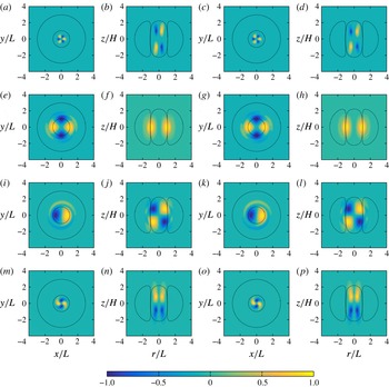
1 Introduction
Coherent vortices are prominent features of geophysical and astrophysical turbulent flows. Examples include the oceanic vortices such as Gulf Stream rings (Olson Reference Olson1991) and Mediterranean eddies (Meddies) (McWilliams Reference McWilliams1985; Armi et al. Reference Armi, Hebert, Oakey, Price, Richardson, Rossby and Ruddick1988) and similar vortices in other regions including the Ulleung Basin, Red Sea, and bay of Biscay (Meschanov & Shapiro Reference Meschanov and Shapiro1998; Carton Reference Carton2001; Chang et al. Reference Chang, Teague, Lyu, Perkins, Lee, Watts, Kim, Mitchell, Lee and Kim2004), as well as vortices in the atmosphere of gas giants such as Jupiter and Saturn (Marcus Reference Marcus1993; Vasavada & Showman Reference Vasavada and Showman2005; O’Neill, Emanuel & Flierl Reference O’Neill, Emanuel and Flierl2015), extreme-weather-causing blocking anticyclones in the Earth’s atmosphere (Tyrlis & Hoskins Reference Tyrlis and Hoskins2008; Hassanzadeh, Kuang & Farrell Reference Hassanzadeh, Kuang and Farrell2014; Hassanzadeh & Kuang Reference Hassanzadeh and Kuang2015) and vortices in the protoplanetary disks where stars and planets form (Barge & Sommeria Reference Barge and Sommeria1995; Barranco & Marcus Reference Barranco and Marcus2005; Marcus et al. Reference Marcus, Pei, Jiang and Hassanzadeh2013). Understanding the dynamics of these vortices, such as their formation, longevity and stability, is of great interest as these vortices can strongly affect their surroundings, for example by efficiently mixing and transporting heat, momentum and material (Gascard et al. Reference Gascard, Watson, Messias, Olsson, Johannessen and Simonsen2002; Marcus Reference Marcus2004; Dong et al. Reference Dong, McWilliams, Liu and Chen2014; Marcus et al. Reference Marcus, Pei, Jiang, Barranco, Hassanzadeh and Lecoanet2015). Despite their widely different environments and time and length scales, a common aspect of these vortices is that their dynamics is predominantly controlled by the rotation, stratification and (in some cases) shear of their environment.
The linear and nonlinear (i.e. finite-amplitude) stability of vortices in rotating, stratified flows has been extensively studied in the past 30 years. However, the majority of those studies have used idealized models for the vortices or for the governing equations. For example, Ikeda (Reference Ikeda1981), Helfrich & Send (Reference Helfrich and Send1988) and Benilov (Reference Benilov2005b ) studied quasi-geostrophic (QG) vortices in discrete two-layer flows; Gent & McWilliams (Reference Gent and McWilliams1986) studied columnar (i.e. with no variation in the vertical direction) QG vortices; Flierl (Reference Flierl1988) examined columnar and three-dimensional (3-D) QG vortices; Nguyen et al. (Reference Nguyen, Hua, Schopp and Carton2012) studied 3-D QG vortices; Carton & McWilliams (Reference Carton, McWilliams, Nihoul and Jamart1989) investigated one- and two-layer QG vortices; Dewar & Killworth (Reference Dewar and Killworth1995), Killworth, Blundell & Dewar (Reference Killworth, Blundell and Dewar1997), Dewar, Killworth & Blundell (Reference Dewar, Killworth and Blundell1999), Baey & Carton (Reference Baey and Carton2002), Benilov (Reference Benilov2004), Benilov (Reference Benilov2005a ), Benilov & Flanagan (Reference Benilov and Flanagan2008), Lahaye & Zeitlin (Reference Lahaye and Zeitlin2015) and Benilov, Broutman & Kuznetsova (Reference Benilov, Broutman and Kuznetsova1998) examined two-layer ageostrophic vortices (the latter also studied geostrophic vortices); Katsman et al. (Reference Katsman, Van der Vaart, Dijkstra and De Ruijter2003) examined multilayer ageostrophic vortices; Smyth & McWilliams (Reference Smyth and McWilliams1998), Billant, Dritschel & Chomaz (Reference Billant, Dritschel and Chomaz2006) and Yim & Billant (Reference Yim and Billant2015) studied columnar ageostrophic vortices; Stegner & Dritschel (Reference Stegner and Dritschel2000) examined shallow-water ageostrophic vortices; Lazar et al. (Reference Lazar, Stegner, Caldeira, Dong, Didelle and Viboud2013a ) and Lazar, Stegner & Heifetz (Reference Lazar, Stegner and Heifetz2013b ) studied shallow-water inertially unstable vortices; Sutyrin (Reference Sutyrin2015) examined two- and three-layer ageostrophic vortices; Brunner-Suzuki, Sundermeyer & Lelong (Reference Brunner-Suzuki, Sundermeyer and Lelong2012) investigated the evolution of 3-D ageostrophic vortices (but this was not technically a stability study because the initial vortices were created through geostrophic adjustment and thus out of equilibrium); and Tsang & Dritschel (Reference Tsang and Dritschel2015) also studied the evolution, rather than the stability, of 3-D ageostrophic vortices made from piecewise-constant elements of potential vorticity that were not exact equilibrium solutions of their equations of motion. One study focused on 3-D equilibrium vortices using the full 3-D Boussinesq equation is that of Yim, Billant & Ménesguen (Reference Yim, Billant and Ménesguen2016) who examined the linear stability of a specific family of vortices with Gaussian angular velocity.
Two of the main motivations for some of the studies listed above have been (i) the observed stability of the long lived, approximately axisymmetric vortices in the oceans and (ii) the observed cyclone–anticyclone asymmetry in the oceans and planetary atmospheres. It has been observed through tracking individual vortices and by satellite observations that coherent oceanic vortices with radii of tens to hundreds of kilometres can last for months and even years (
 ${\sim}1/2{-}3$
) while remaining nearly axisymmetric (Lai & Richardson Reference Lai and Richardson1977; Armi et al.
Reference Armi, Hebert, Oakey, Price, Richardson, Rossby and Ruddick1989; Olson Reference Olson1991; Chelton, Schlax & Samelson Reference Chelton, Schlax and Samelson2011). However, most theoretical studies of axisymmetric vortices in rotating stratified flows have found them to be linearly unstable (usually with fast growth rates that are incompatible with the observed longevity of these vortices), unless unrealistic parameters or vertical structures are assumed (see the discussions in Stegner & Dritschel Reference Stegner and Dritschel2000; Benilov Reference Benilov2004, Reference Benilov2005b
; Sutyrin Reference Sutyrin2015). Observations of planetary atmospheres (Mac Low & Ingersoll Reference Mac Low and Ingersoll1986; Cho & Polvani Reference Cho and Polvani1996), and oceans at the mesoscales (McWilliams Reference McWilliams1985; Chelton et al.
Reference Chelton, Schlax, Samelson and de Szoeke2007, Reference Chelton, Schlax and Samelson2011; Mkhinini et al.
Reference Mkhinini, Coimbra, Stegner, Arsouze, Taupier-Letage and Béranger2014) show that long-lived vortices are predominantly anticyclones. Whether this asymmetry is due to differences between the stability (linear or nonlinear) properties of cyclones and anticyclones requires a better understanding of how stability changes with the Rossby number. It should be noted that factors other than stability can be responsible for, or at least contribute to, the observed cyclone–anticyclone asymmetry; for example the creation mechanisms might favour anticyclones (Perret, Dubos & Stegner Reference Perret, Dubos and Stegner2011), anticyclones might decay slower than cyclones (Hoskins, McIntyre & Robertson Reference Hoskins, Mcintyre and Robertson1985, § 7; Graves, McWilliams & Montgomery Reference Graves, McWilliams and Montgomery2006) or coherent cyclones might be harder to observe in planetary atmospheres than anticyclones (Marcus Reference Marcus2004).
While valuable information on the stability of vortices in rotating stratified flows, vortices in planetary atmospheres and oceanic eddies has been gained through the aforementioned studies, further investigation of the linear and nonlinear stability that extends beyond the simplifications and limitations of these studies is still needed. In the current study, we address the stability of isolated, 3-D, axisymmetric vortices in rotating, stably stratified, inviscid flows by analysing the full non-hydrostatic Boussinesq equations with an
 $f$
-plane approximation in a 3-D domain with periodic boundary conditions (modified to simulate an unbounded flow). We focus on a widely used model of geophysical and astrophysical vortices, which have pressure anomalies that are Gaussian in the radial and vertical directions and are in exact equilibrium (e.g. McWilliams Reference McWilliams1985; van Heijst & Clercx Reference van Heijst and Clercx2009; Chelton et al.
Reference Chelton, Schlax and Samelson2011; Hassanzadeh, Marcus & Le Gal Reference Hassanzadeh, Marcus and Le Gal2012). Our work extends the analyses of the previous studies in several ways, including:
-
(i) By using the Boussinesq equations, we can study vortex dynamics with any Rossby number and internal stratification. Here we focus on cyclones and anticyclones in the geostrophic balance regime (
 $-0.5<Ro<0.5$
), which is the range of
$Ro$
relevant to most long-lived geophysical and astrophysical vortices (e.g. Olson Reference Olson1991; Aubert et al.
Reference Aubert, Le Bars, Le Gal and Marcus2012) (all parameters and dimensionless numbers are defined in § 2). The vertical stratification inside the 3-D equilibrium vortices that are studied here can be much stronger or much weaker compared to the stratification of the background (i.e. far from the vortex) flow, which is also the case for many oceanic and atmospheric vortices (e.g. Aubert et al.
Reference Aubert, Le Bars, Le Gal and Marcus2012). Considering vortices with finite Rossby numbers and with internal stratifications that significantly differ from the stratification of the background flow extends the stability analysis well beyond the QG approximation.
-
(ii) Geophysical and astrophysical vortices that are far from both horizontal and vertical boundaries (e.g. free surfaces or solid surfaces) and that are in quasi-equilibrium have been observed to be three-dimensional (rather than 2-D Taylor columns); examples include Jupiter’s Great Red Spot (Marcus Reference Marcus1993), Meddies (Aubert et al. Reference Aubert, Le Bars, Le Gal and Marcus2012; Bashmachnikov et al. Reference Bashmachnikov, Neves, Calheiros and Carton2015) and zombie vortices in the protoplanetary disks (Barranco & Marcus Reference Barranco and Marcus2005; Marcus et al. Reference Marcus, Pei, Jiang and Hassanzadeh2013, Reference Marcus, Pei, Jiang, Barranco, Hassanzadeh and Lecoanet2015). The vertical length scales of these vortices are finite and usually much smaller than their horizontal length scales, which can be understood as a direct consequence of the gradient–wind balance (see Hassanzadeh et al. Reference Hassanzadeh, Marcus and Le Gal2012). The present study extends the rigorous stability analysis of Boussinesq vortices beyond barotropic Taylor columns.
-
(iii) Exploiting the universal scaling law of Aubert et al. (Reference Aubert, Le Bars, Le Gal and Marcus2012) and Hassanzadeh et al. (Reference Hassanzadeh, Marcus and Le Gal2012), the 3-D baroclinic vortices studied here are exact equilibrium solutions of the full 3-D non-hydrostatic Boussinesq equations (see § 2.3). The exact equilibrium is particularly important for a rigorous linear analysis, which is the subject of this paper.
-
(iv) By using the full, 3-D, non-hydrostatic Boussinesq equations, we avoid restrictions on the vertical structure of the vortex or background flow that result from the QG or multilayer models discussed above. Although here we focus on background flows with stable stratification such that the density decreases linearly with height (i.e. constant Brunt–Väisälä frequency
$\bar{N}$
), background flows with more realistic
$\bar{N}(z)$
profiles can be easily included in this framework. -
(v) The family of Gaussian vortices that is studied here has been shown to fit many types of oceanic and laboratory vortices reasonably well (e.g. van Heijst & Clercx Reference van Heijst and Clercx2009; Chelton et al. Reference Chelton, Schlax and Samelson2011) and has been widely used as a model in various theoretical studies (e.g. McWilliams Reference McWilliams1985; Morel & McWilliams Reference Morel and McWilliams1997; Hassanzadeh et al. Reference Hassanzadeh, Marcus and Le Gal2012; Negretti & Billant Reference Negretti and Billant2013). Furthermore in this model, all fields (e.g. velocity, potential vorticity and density) are continuous and smooth, which eliminate unphysical instabilities that can arise from discontinuities (which are present, for example, when vortices are modelled with piecewise-constant shells or patches of potential vorticity).


In this paper we address the linear stability of 3-D vortices in rotating stratified flows and discuss the growth rates and most unstable eigenmodes as functions of the Rossby number
 $Ro$
(for
 $-0.5<Ro<0.5$
), the Burger number
 $Bu$
(for
 $0.02<Bu<2.3$
) and
 $f/\bar{N}=0.1$
and
 $0.01$
. One of the main purposes of this paper is to extend the linear stability analysis of a specific family of 3-D equilibrium vortices beyond some of the approximations or constraints imposed in previous studies and produce the parameter map of stability for 3-D non-hydrostatic Boussinesq flows. We also investigate how different modes take over as the most unstable one as the Burger number changes and explore the vertical and horizontal structures of these modes and their critical layers. We discuss how the stability properties found here compare with those reported in other studies using QG or multilayer equations or using a different vortex model. Furthermore, we show numerically that the linear stability of the family of 3-D vortices that we examine is only weakly dependent on the value of
 $f/\bar{N}$
for
 $f/\bar{N}\leqslant 0.1$
and we discuss the reason behind this behaviour.
The results of this paper improve the understanding of the generic stability properties of 3-D vortices in rotating stratified flows, and have implications for the dynamics of some of the geophysical and astrophysical vortices. These results are most relevant to the stability of interior (i.e. far from boundaries) oceanic vortices such as Meddies. It is acknowledged that the exclusion of horizontal and vertical background shear, free surface, lateral boundaries, bottom topography, compressible effects and vertical variation of
 $\bar{N}$
limit the direct applicability of the current analysis to other oceanic eddies and planetary and astrophysical vortices. However, the numerical framework presented here can be readily adapted to account for the aforementioned boundary conditions/physical processes in future studies, and the results of this paper will be needed to evaluate the influence of these boundary conditions/processes on the stability properties of these vortices.
The remainder of this paper is structured as follows. The equations of motion, numerical method, Gaussian vortex model and eigenmode solver are discussed in § 2. The eigenmodes with critical layers are discussed in § 3 and the results of the linear stability analysis and the stability map along with comparison with previous studies are presented in § 4. Insensitivity of the most unstable modes to
 $f/\bar{N}$
is discussed in § 5 and the radial and vertical structures of the most unstable modes are presented in § 6. Discussion and summary are in § 7.
2 Problem formulation
2.1 Equations of motion
The Boussinesq approximation of the equations of motion for 3-D rotating, stratified, inviscid flows in the Cartesian coordinates
 $(x,y,z)$
, as observed in a frame rotating with angular velocity
 $(f/2)\hat{\boldsymbol{z}}$
, is (Vallis Reference Vallis2006)
 $$\begin{eqnarray}\displaystyle \frac{\text{D}\boldsymbol{v}}{\text{D}t}=-\frac{\unicode[STIX]{x1D735}p}{\unicode[STIX]{x1D70C}_{o}}+\boldsymbol{v}\times f\hat{\boldsymbol{z}}+b\hat{\boldsymbol{z}},\quad \frac{\text{D}b}{\text{D}t}=-\bar{N}^{2}v_{z},\quad \unicode[STIX]{x1D735}\boldsymbol{\cdot }\boldsymbol{v}=0, & & \displaystyle\end{eqnarray}$$
where the operator
 $\text{D}/\text{D}t\equiv \unicode[STIX]{x2202}/\unicode[STIX]{x2202}t+\boldsymbol{v}\boldsymbol{\cdot }\unicode[STIX]{x1D735}$
is the material derivative,
 $t$
denotes time,
 $\boldsymbol{v}=(v_{x},v_{y},v_{z})$
is the 3-D velocity vector,
 $f$
is the Coriolis frequency (constant in our study) and
 $g$
is the acceleration of gravity. The total pressure and the total density of the fluid are
 $p_{tot}\equiv \bar{p}(z)+p(x,y,z,t)$
and
 $\unicode[STIX]{x1D70C}_{tot}\equiv \bar{\unicode[STIX]{x1D70C}}(z)+\unicode[STIX]{x1D70C}(x,y,z,t)$
, where
 $\bar{\unicode[STIX]{x1D70C}}(z=0)=\unicode[STIX]{x1D70C}_{o}$
. We define the buoyancy as
 $b(x,y,z,t)\equiv -g\unicode[STIX]{x1D70C}/\unicode[STIX]{x1D70C}_{o}$
. Quantities with a bar are properties of the equilibrium background flow (i.e. far from the vortex where
 $\boldsymbol{v}\rightarrow 0$
,
 $b\rightarrow 0$
,
 $\unicode[STIX]{x1D70C}\rightarrow 0$
and
 $p\rightarrow 0$
). The background pressure
 $\bar{p}$
and density
 $\bar{\unicode[STIX]{x1D70C}}$
are in hydrostatic balance
 $\text{d}\bar{p}/\text{d}z=-\bar{\unicode[STIX]{x1D70C}}g$
. The background Brunt–Väisälä frequency
 $\bar{N}\equiv \sqrt{-(g/\unicode[STIX]{x1D70C}_{o})(\text{d}\bar{\unicode[STIX]{x1D70C}}/\text{d}z)}$
is assumed to be constant, so that
 $\bar{\unicode[STIX]{x1D70C}}(z)=\unicode[STIX]{x1D70C}_{o}(1-\bar{N}^{2}z/g)$
.
In the above equations, we have ignored viscosity in the momentum equations and diffusion in the density equation, which are reasonable approximations for atmospheric and oceanic flows. Furthermore, we have dropped the planetary centrifugal term from the momentum equations, assuming that the rotational Froude number
 $f^{2}d/g$
is small (Barcilon & Pedlosky Reference Barcilon and Pedlosky1967), where
 $d$
is the distance between the centre of the vortex and the planetary rotation axis.
2.2 Numerical method
A pseudo-spectral initial-value solver is developed to solve (2.1) in a triply periodic domain with 256 or 512 Fourier modes in each direction. In numerical simulations of strongly rotating stratified flows, resolving the fast inertia–gravity waves can substantially limit the size of the time step
 $\unicode[STIX]{x0394}t$
and thus increase the computational cost. Here we use the semi-analytic method developed by Barranco & Marcus (Reference Barranco and Marcus2006) for rotating stratified flows, which enables us to accurately and efficiently deal with large
 $f\unicode[STIX]{x0394}t$
and
 $\bar{N}\unicode[STIX]{x0394}t$
.
A vortex in the middle of a periodic domain interacts with its periodic images. To minimize this interaction and its potential impact on the stability of the vortex (and to simulate having an unbounded flow) the computational domain size is chosen to be large compared to the vortex size: the domain size in the
 $x$
and
 $y$
directions, i.e. the values of
 $L_{x}$
and
 $L_{y}$
are 7.5 (or more often 15) times larger than the initial vortex diameter
 $(2L)$
, and, similarly, the domain size in the
 $z$
direction
 $L_{z}$
is 7.5 (or more often 15) times larger than the initial vortex height
 $(2H)$
. There are two reasons for sometimes making the domain size very large. First, we wanted to ensure that the periodic boundary conditions had no perceptible effects on the flow dynamics; secondly, in the follow-up paper to this one (see our discussion § 7) we show that unstable vortices often fragment with pieces of the initial vortices becoming widely separated, so that the calculations require a large domain. To help simulate an unbounded flow, we also added a cylindrical sponge layer near the boundaries of the computational domain (see appendix A). The sponge layer, implemented as Rayleigh drag and Newtonian cooling in (2.1), damps
 $\boldsymbol{v}$
and
 $\unicode[STIX]{x1D70C}$
outside a cylindrical surface of diameter
 $24L$
and height
 $24H$
(for the large domain calculations) or
 $12L$
and height
 $12H$
(for the small domain calculations) around the centre of the domain. Another advantage of adding the sponge layer is that it damps the reflection of the outgoing inertia–gravity waves, and occasional detached filaments back to the domain at the periodic boundaries. One more advantage of the axisymmetric sponge layer is that we find that it prevents the (non-axisymmetric) periodic boundary conditions in
 $x$
and
 $y$
from adding any significant non-axisymmetric perturbations to the initial vortices. The latter is important when computing the stability of the vortices. One way of determining if the domain size is too small is to compute the ratio of the magnitude of each component of the velocity and density of a numerically computed eigenmode at a damped location just inside the sponge layer to the maximum value of that component over the entire domain. With the domain sizes presented here, that ratio is always of order
 $10^{-4}$
(or smaller), but the ratio increases to values with orders as large as
 $10^{-2}$
when the computational domain is reduced to
 $(10L)\times (10L)\times (10H)$
and a sponge layer with diameter of
 $8L$
and height
 $8H$
.
Hyperviscosities and hyperdiffusivities are added to our otherwise inviscid and non-diffusive calculations to stabilize the code. See Barranco & Marcus (Reference Barranco and Marcus2006) for more details.
2.3 Initial equilibria: Gaussian vortices
In this study we focus on 3-D axisymmetric baroclinic vortices that are initially in horizontal cyclo-geostrophic balance and vertical hydrostatic balance, and hence they are in gradient–wind balance (Vallis Reference Vallis2006). The initial vortex is centred at
 $r=0$
and
 $z=0$
, where
 $r$
denotes the radial coordinate. A widely used model for oceanic and laboratory vortices is that of an axisymmetric vortex with a Gaussian pressure distribution (e.g. McWilliams Reference McWilliams1985)
 $$\begin{eqnarray}\displaystyle p=p_{o}\unicode[STIX]{x1D712}(r,z), & & \displaystyle\end{eqnarray}$$
where
 $\unicode[STIX]{x1D712}(r,z)\equiv \exp [-(r/L)^{2}-(z/H)^{2}]$
. Using (2.2) and the definitions presented in § 2.1, an exact, steady, axisymmetric equilibrium solution to the Boussinesq equations in (2.1) is the vortex
 $$\begin{eqnarray}\displaystyle & \displaystyle v_{\unicode[STIX]{x1D719}}(r,z)={\displaystyle \frac{fr}{2}}\left(-1+\sqrt{1-(8p_{o}\unicode[STIX]{x1D712}(r,z))/(\unicode[STIX]{x1D70C}_{o}f^{2}L^{2})}\right),\quad v_{r}=v_{z}=0, & \displaystyle\end{eqnarray}$$
 $$\begin{eqnarray}\displaystyle & \displaystyle b(r,z)=-{\displaystyle \frac{2p_{o}z}{\unicode[STIX]{x1D70C}_{o}H^{2}}}\unicode[STIX]{x1D712}(r,z), & \displaystyle\end{eqnarray}$$
where the cylindrical coordinate is used for convenience (
 $v_{\unicode[STIX]{x1D719}}$
is the azimuthal velocity). For any vortex, whether or not it is Gaussian, we shall define a quantity written with a subscript ‘
 $c$
’ to mean that the quantity is to be evaluated at the vortex centre, so
 $N_{c}$
is the Brunt–Väisälä frequency at the centre of a vortex, or
 $N_{c}^{2}\equiv \bar{N}^{2}+(\unicode[STIX]{x2202}b/\unicode[STIX]{x2202}z)_{c}$
. For the Gaussian vortex described by (2.3)–(2.4),
 $$\begin{eqnarray}\displaystyle N_{c}^{2}=\bar{N}^{2}-2p_{o}/(\unicode[STIX]{x1D70C}_{o}H^{2}). & & \displaystyle\end{eqnarray}$$
As discussed in the next section, for some values of
 $p_{o}$
,
 $N_{c}^{2}<0$
, which means that the density distribution is locally unstable at the vortex centre with heavy fluid over light fluid (i.e. statically unstable). It is convenient to define the Rossby number
 $Ro$
, which by definition has
 $Ro>0$
for a cyclone and
 $Ro<0$
for an anticyclone, in terms of the maximum (or minimum) value of a vortex’s vertical vorticity
 $\unicode[STIX]{x1D714}_{E}$
, such that
 $Ro\equiv \unicode[STIX]{x1D714}_{E}/2f$
. For the Gaussian vortices described above
 $\unicode[STIX]{x1D714}_{E}=\unicode[STIX]{x1D714}_{c}$
, and
 $$\begin{eqnarray}Ro=\unicode[STIX]{x1D714}(r=0,z=0)/2f=-1/2+\sqrt{1/4-2p_{o}/(\unicode[STIX]{x1D70C}_{o}f^{2}L^{2})}.\end{eqnarray}$$
Note that the Gaussian vortex has an aspect ratio of
 $$\begin{eqnarray}\left(\frac{H}{L}\right)^{2}=\frac{-Ro(1+Ro)f^{2}}{\bar{N}^{2}[1-(N_{c}/\bar{N})^{2}]},\end{eqnarray}$$
in accord with the universal scaling law of Aubert et al. (Reference Aubert, Le Bars, Le Gal and Marcus2012) and Hassanzadeh et al. (Reference Hassanzadeh, Marcus and Le Gal2012), which is valid for all vortices that are in cyclo-geostrophic and hydrostatic balance. This can be seen by simply replacing
 $2p_{o}/\unicode[STIX]{x1D70C}_{o}$
in (2.6) with
 $H^{2}(\bar{N}^{2}-N_{c}^{2})$
using (2.5), and then solving for
 $H/L$
.
The three independent dimensional parameters in the governing equations (2.1) are
 $f$
,
 $\bar{N}$
and
 $\unicode[STIX]{x1D70C}_{o}$
. The sizes of the computational domain
 $L_{x}\times L_{y}\times L_{z}$
have no effect (on the dimensional analysis), due to the fact that the cylindrical sponge layer is far from the vortices and that the net circulations of the flow are zero, which makes the velocity due to the vortices fall off exponentially fast and be effectively zero at the sponge layer. (See the definition of shielded below and in the appendices.) The equilibrium Gaussian vortices in (2.2)–(2.4) introduce three additional dimensional parameters
 $H$
,
 $L$
and
 $p_{o}$
. Thus, there are three independent, dimensionless parameters that describe the dynamics of Gaussian vortices. The choice of these parameters is not unique, but in this paper we choose
 $Ro$
,
 $f/\bar{N}$
, and
 $$\begin{eqnarray}Bu\equiv \left(\frac{\bar{N}}{f}\frac{H}{L}\right)^{2}=(L_{r}/L)^{2},\end{eqnarray}$$
where the latter is the Burger number and
 $L_{r}\equiv H\bar{N}/f$
is the deformation radius. It should be noted that whether the vortices studied here are big or small depends on the inverse of their Burger number, which is the square of the vortex radius over
 $L_{r}$
. Big vortices have small
 $Bu$
and vice versa.
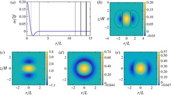
Vertical vorticity
 $\unicode[STIX]{x1D714}(r,z)$
and potential vorticity
 $Q(r,z)$
for Gaussian cyclones defined by (2.2)–(2.4). Panel (a) shows
 $\unicode[STIX]{x1D714}$
at
 $z=0$
as a function of
 $r$
as a solid curve (blue, in colour) for
 $Ro=0.2$
,
 $Bu=0.1$
and
 $f/\bar{N}=0.1$
. The thin and thick dashed vertical lines show the boundaries of the core and the shield (see appendix B). The solid vertical lines at large radii show, with increasing thickness from left to right, where the boundary damping function
 $f_{bd}$
(see appendix A) reaches values of 0.01, 0.5 and 0.99, respectively. Panel (b) shows
 $\unicode[STIX]{x1D714}(r,z)$
in units of
 $2f$
in the
 $r$
–
 $z$
plane of the vortex in (a). Dashed lines indicate the boundaries of the core and shield. (c–e) Show the potential vorticity
 $Q(r,z)$
for a Gaussian vortex with
 $Ro=0.2$
and
 $f/\bar{N}=0.1$
, for
 $Bu=0.1$
,
 $Bu=1.0$
and
 $Bu=2.0$
, respectively. For larger values of
 $Bu$
, the distributions of
 $Q$
and
 $\unicode[STIX]{x1D714}$
are similar.

The Gaussian vortices defined in the above model are shielded. Here we define a shielded flow as one in which the circulation computed with the
 $z$
-component of the vorticity over the entire
 $(x,y)$
-plane for any fixed value of
 $z$
is zero. In addition, the circulation computed with the
 $x$
-component of the vorticity over the
 $(y,z)$
-plane for any fixed value of
 $x$
is zero; and the circulation computed with the
 $y$
-component of the vorticity over the
 $(x,z)$
-plane for any fixed value of
 $y$
is zero. (Note that figure 1(b) does not violate our definition of shielded because the figure shows the vertical component of the vorticity in an
 $x$
–
 $z$
plane, not an
 $x$
–
 $y$
plane.) Our governing equations and boundary conditions show that if the initial flow is shielded, then the flow is shielded for all time. In practical terms, a shielded isolated vortex is one in which the central core of the vortex is surrounded, or partially surrounded, by a region (shield) of opposite vorticity and that the circulation quickly vanishes outside the shield. For an arbitrary (i.e. not necessarily Gaussian) cyclonic vortex, the core of a cyclone is a contiguous region at and near the vortex centre where the vertical component of its vorticity
 $\unicode[STIX]{x1D714}$
is greater than or equal to zero. The shield is a region around the core (usually looking like a shell or annular ring) located not too far from the core, where
 $\unicode[STIX]{x1D714}<0$
. The precise definitions that we use for core and shield are in appendix B. The core and shield of an example Gaussian vortex are illustrated in figure 1(a,b). The definitions of the core and shield of an anticyclone are analogous to those of the cyclone. For Gaussian vortices and many other types of shielded cyclones, outside the shield the amplitude of the vorticity decays exponentially with the radial distance
 $r$
(or
 $r^{p}$
with
 $p\geqslant 2$
) from the vortex centre. In our calculations, the circulation due to the vertical component of the vorticity
 $\int \unicode[STIX]{x1D714}(x,y,z)\,\text{d}x\,\text{d}y$
(where the integral is over the entire
 $x$
–
 $y$
computational domain) at each value of
 $z$
must remain zero due to the periodic boundary conditions.
Commonly, in the studies of oceanic and atmospheric vortices, potential vorticity (PV) is used to describe the vortices, instead of vertical vorticity, due to its conservation property (Hoskins et al. Reference Hoskins, Mcintyre and Robertson1985; Morel & McWilliams Reference Morel and McWilliams1997). Ertel’s PV in figure 1 is defined (Ertel Reference Ertel1942) as
 $$\begin{eqnarray}Q\equiv [\unicode[STIX]{x1D74E}+f\hat{\boldsymbol{z}}]\boldsymbol{\cdot }\left(\frac{\unicode[STIX]{x1D735}b+\bar{N}^{2}\hat{\boldsymbol{z}}}{f\bar{N}^{2}}\right)-1,\end{eqnarray}$$
where
 $\unicode[STIX]{x1D74E}\equiv \unicode[STIX]{x1D735}\times \boldsymbol{v}$
is the vorticity vector as observed in the rotating frame. To provide a better sense about the PV structure of the vortices studied here,
 $Q(r,z)$
for a Gaussian vortex with
 $Ro=0.2$
and three values of
 $Bu=0.1,1$
and
 $2$
are depicted in figure 1(c–e), showing that the PV structure can significantly change with
 $Bu$
(see Morel & McWilliams (Reference Morel and McWilliams1997) for a discussion of potential vorticity of Gaussian vortices). Our purpose for showing the PV of Gaussian vortices is to allow the reader the ability to make comparisons of the vortex model with what is used in some other stability studies such as Tsang & Dritschel (Reference Tsang and Dritschel2015) who model the initial vortex with uniform patches of PV.
Finally it should be noted that there is a restriction on the equilibrium of anticyclones in the Gaussian model (2.2)–(2.4); there is no equilibrium for anticyclones for
 $Ro<-0.5$
. This is because (2.3) and (2.6) show that
 $v_{\unicode[STIX]{x1D719}}$
does not have a real solution for
 $Ro<-0.5$
, as noted, for example, by McWilliams (Reference McWilliams1985) and Olson (Reference Olson1991).
2.4 Eigenmodes
The symmetries of the governing equations in (2.1) linearized around the equilibrium vortex (2.2)–(2.4) are presented in dimensionless form in § 5 in (5.10)–(5.14). These equations and their boundary conditions show that the eigenfunctions are either symmetric or antisymmetric with respect to the
 $z=0$
horizontal plane and have an
 $m$
-fold azimuthal symmetry about the
 $z$
-axis. We use the labels S
 $m$
or A
 $m$
for each eigenmode, to identify it as symmetric (or antisymmetric) with respect to the
 $z=0$
horizontal plane and with
 $m$
-fold symmetry.
The complex eigenvalues
 $\unicode[STIX]{x1D706}$
and eigenfunctions are of the form
 $$\begin{eqnarray}\text{e}^{\unicode[STIX]{x1D706}t}\boldsymbol{g}_{eig}(r,z)\text{e}^{\text{i}m\unicode[STIX]{x1D719}}=\text{e}^{\unicode[STIX]{x1D70E}t}\boldsymbol{g}_{eig}(r,z)\text{e}^{\text{i}m(\unicode[STIX]{x1D719}-ct)},\end{eqnarray}$$
where the eigenvector has three velocity components, a density component and a pressure component:
 $$\begin{eqnarray}\boldsymbol{g}_{eig}(r,z)\equiv [v_{r,eig},v_{\unicode[STIX]{x1D719},eig},v_{z,eig},\unicode[STIX]{x1D70C}_{eig},p_{eig}].\end{eqnarray}$$
The three velocity components are with respect to cylindrical coordinates, where
 $m$
is the integer azimuthal wavenumber,
 $\unicode[STIX]{x1D70E}$
is a real growth (or decay) rate and
 $c$
is a real azimuthal phase speed. By taking the complex conjugate of the linearized equation, we can show that if
 $\unicode[STIX]{x1D706}$
is an eigenvalue with eigenfunction given by (2.11), then
 $\unicode[STIX]{x1D706}^{\dagger }$
is also an eigenvalue with eigenfunction
 $\boldsymbol{g}_{eig}^{\dagger }(r,z)\equiv [v_{r,eig}^{\dagger },v_{\unicode[STIX]{x1D719},eig}^{\dagger },v_{z,eig}^{\dagger },\unicode[STIX]{x1D70C}_{eig}^{\dagger },p_{eig}^{\dagger }]$
, with
 $m$
replaced by
 $-m$
,
 $c$
unchanged and where the superscript
 $\dagger$
denotes complex conjugate. Or in other words, the eigenvalues
 $\unicode[STIX]{x1D706}$
when plotted in the complex plane are symmetric with respect to the real axis. Because the equations are non-dissipative, replacing
 $t$
with
 $-t$
in the linearized equations shows that if
 $\unicode[STIX]{x1D706}\equiv \unicode[STIX]{x1D70E}-\text{i}mc$
is an eigenvalue with eigenfunction given by (2.11), then
 $\unicode[STIX]{x1D706}^{\prime }\equiv -\unicode[STIX]{x1D70E}-\text{i}m^{\prime }c^{\prime }$
is an eigenvalue that corresponds to
 $\boldsymbol{g}_{eig}^{\prime }(r,z)\equiv [v_{r,eig},-v_{\unicode[STIX]{x1D719},eig},v_{z,eig},-\unicode[STIX]{x1D70C}_{eig},-p_{eig}]$
, with
 $m^{\prime }=-m$
and
 $c^{\prime }=c$
. Or in other words, the eigenvalues
 $\unicode[STIX]{x1D706}$
when plotted in the complex plane are symmetric with respect to the imaginary axis and for each eigenfunction with a positive growth rate there is one with a negative growth rate and vice versa. The flow can never be linearly stable with all of its eigenmodes having decay rates. The flow can either be unstable or be neutrally stable with all of its eigenmodes on the imaginary axis with
 $\unicode[STIX]{x1D70E}=0$
. For the Gaussian vortices, the two symmetries of the linearized equations combine and therefore the eigenvalues appear as quartets of the form
 $\pm a\pm \text{i}b$
, with all four possible combinations of the signs, and where
 $a$
and
 $b$
are real functions of
 $m$
and of the parameters of the unperturbed vortex
 $Ro$
,
 $Bu$
and
 $f/\bar{N}$
. For Hamiltonian systems (Ozorio de Almeida Reference Ozorio de Almeida1988), it can be shown that the quartet of eigenvalues is of a more specialized form:
 $$\begin{eqnarray}\unicode[STIX]{x1D706}=\pm \sqrt{A}\pm \text{i}B,\end{eqnarray}$$
with all four possible combinations of the signs, and where
 $A$
and
 $B$
are real functions of the control parameters of the system. For many non-dissipative flows, e.g. unidirectional shears flows with vortex sheets and/or vortex layers made up of piecewise-constant vorticity (Drazin & Reid Reference Drazin and Reid2004), it can be shown that the quartets of the eigenvalues are of the form of (2.12). Consider a system with eigenvalue quartets such as those in (2.12). When
 $A>0$
, the eigenvalues in the quartets are symmetric about the real and imaginary axes and each quartet has two unstable and two stable eigenmodes. If a control parameter changes such that
 $A$
decreases, then eigenvalues symmetrically approach the imaginary axis and collide when
 $A=0$
. For that parameter value, there are two pairs of degenerate, neutrally stable eigenmodes with all four eigenvalues on the imaginary axis. If the control parameter is further changed such that
 $A$
continues to decrease and becomes negative, then the eigenvalues are no longer degenerate, but they remain on the imaginary axis and all four eigenmodes remain neutrally stable, regardless of how negative
 $A$
becomes. Although we cannot prove that the eigenvalue quartets of the linear eigenmodes of the Gaussian vortex have the form of (2.12), all of our numerical simulations are consistent with (2.12). (See § 3.)
Note that although we are studying the stability of axisymmetric vortices, we solve (2.1) in the Cartesian coordinates rather than in the cylindrical coordinates. A numerical solver in the Cartesian coordinates avoids the difficulties of handling the singularity at the origin (
 $r=0$
), which requires using special polynomial basis functions (Matsushima & Marcus Reference Matsushima and Marcus1995). However, our main reason for using Cartesian coordinates is that future studies can include background shear flows, so that the stability of vortices in planetary atmospheres and protoplanetary disks can be examined, as discussed in the Introduction. To minimize the effect of the square computational domain, we have used a circular sponge layer as described in § 2.2. In order to find the eigenmodes with various classes of azimuthal (and vertical) symmetry in the Cartesian coordinates, we use our initial-value solver as an eigenvector/eigenvalue solver and additionally use a spatial symmetrizer (see appendix C for details). Using the spatial symmetrizer, the eigenmodes can be restricted to be symmetric or antisymmetric in the vertical direction, while in the azimuthal direction we can enforce one of the following classes of symmetry:
 $m$
odd;
 $m$
even not divisible by
 $4$
; and
 $m$
even and divisible by
 $4$
. We use these specific symmetry groups to apply the azimuthal symmetry directly in the Cartesian coordinates, which greatly speeds up the convergence of the calculations, and also avoids introducing additional errors due to transformation between Cartesian and cylindrical coordinates (see appendix C).
3 Critical layers
Eigenmodes of unidirectional equilibrium flows, such as the Gaussian vortices studied here, can have critical layers, i.e. singularities at locations where the azimuthal phase speed
 $c$
is equal to the azimuthal velocity
 $v_{\unicode[STIX]{x1D719}}(r,z)$
of the unperturbed vortex (Maslowe Reference Maslowe1986; Benilov Reference Benilov2003). (In stratified unidirectional flows, critical layers can appear at other locations as well (Marcus et al.
Reference Marcus, Pei, Jiang and Hassanzadeh2013, Reference Marcus, Pei, Jiang, Barranco, Hassanzadeh and Lecoanet2015).) Here we show examples of eigenmodes with critical layers and discuss, for a few cases, how different modes take over as the fastest-growing mode as
 $Bu$
changes, which will be used later to interpret the results of § 4. It should be noted that despite the peculiar nature of critical layers, it is not difficult to accurately compute them using high-resolution numerical simulations. For example, Nguyen et al. (Reference Nguyen, Hua, Schopp and Carton2012) and Yim et al. (Reference Yim, Billant and Ménesguen2016) have simulated critical layers in 3-D QG and Boussinesq vortices, respectively. Recently, we have numerically computed critical layers, with and without dissipation, in stratified, rotating, unidirectional flows and found that with sufficient spatial resolution the locations, widths and other analytically known properties of the critical layers can be quantitatively reproduced (Marcus et al.
Reference Marcus, Pei, Jiang and Hassanzadeh2013, Reference Marcus, Pei, Jiang, Barranco, Hassanzadeh and Lecoanet2015). In the results presented here, the location of the critical layers and the phase speed of the eigenmode containing the critical layer are insensitive to the numerical resolution and remain the same when the resolution is increased by a factor of 4 by halving the domain size in each direction to
 $(15L)\times (15L)\times (15H)$
and increasing the Fourier modes from
 $256^{3}$
to
 $512^{3}$
(the figures showing the structure of the eigenmodes in this section are from the higher resolution).
The singularity in the eigenmode occurs where the coefficient
 $[v_{\unicode[STIX]{x1D719}}(r,z)/r-c-\text{i}\unicode[STIX]{x1D70E}/m]$
in front of the highest-order derivative terms in the governing equations of the eigenmode becomes zero. Unless the growth rate
 $\unicode[STIX]{x1D70E}$
is zero and the eigenmode is neutrally stable, the eigenmode is no longer formally singular. However, the amplitudes of the eigenmodes remain large at locations where
 $v_{\unicode[STIX]{x1D719}}(r,z)/r=c$
for parameter values where
 $\unicode[STIX]{x1D70E}>0$
and the mode is weakly growing. For parameter values where the analytically computed eigenmode has
 $\unicode[STIX]{x1D70E}=0$
, but the eigenmode is computed numerically with a modified initial-value code (as done here) with weak hyperdissipation, the computed eigenmode has large amplitude at
 $v_{\unicode[STIX]{x1D719}}(r,z)/r=c$
, and the magnitude of the numerically computed growth rates
 $\unicode[STIX]{x1D70E}$
are typically less than or equal to
 $0.002$
in inverse units of the vortex turnaround time
 $\unicode[STIX]{x1D70F}\equiv 4\unicode[STIX]{x03C0}/\unicode[STIX]{x1D714}_{c}$
, where
 $\unicode[STIX]{x1D714}_{c}$
is the absolute value of the vertical vorticity at the centre of the vortex.
We argued in § 2.4 that as a parameter value, such as the Burger number, is changed such that a growing/decaying pair of eigenmodes has its eigenvalues
 $\unicode[STIX]{x1D706}$
collide on the imaginary axis, the eigenmodes become neutrally stable and degenerate. As the parameter value further changes, the eigenvalues remain neutrally stable and their phase speeds become distinct from each other. Here we demonstrate in detail that this scenario of eigenvalue collision, in which the families of eigenmodes continue after the collision rather than ceasing to exist due to the singularity of the critical layer, is correct by illustrating the collision for three distinct families of eigenmodes with critical layers. In particular, we show that as the
 $Bu$
changes and the eigenmode goes from unstable to neutrally stable, the family containing that eigenmode continues to exist and remains neutrally stable as the
 $Bu$
is further changed. We need these three demonstrations to not only show that our numerical computations of eigenmodes are accurate, but also to highlight the physics of the collisions.
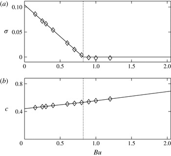
(a) Growth rates
 $\unicode[STIX]{x1D70E}$
(in units of
 $\unicode[STIX]{x1D70F}^{-1}$
) of the eigenmodes with S2 symmetries as functions of
 $Bu$
for
 $Ro=0.05$
and
 $f/\bar{N}=0.1$
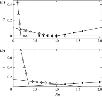
. The lines connecting the symbols are to ‘guide the eye’. The eigenmodes with S2 symmetry are unstable in the range
 $Bu\lesssim 0.823$
(they are the fastest growing for
 $0.2\lesssim Bu\lesssim 0.823$
). As
 $Bu$
increases, the eigenmode changes from unstable to neutrally stable at
 $Bu\simeq 0.823$
(shown with the vertical broken line), but the family of eigenmodes does not terminate there. (b) The phase speed
 $c$
(in units of
 $\unicode[STIX]{x1D70F}^{-1}$
) corresponding to the growth rates shown in (a). The lines connecting the symbols are to guide the eye. The phase speed is continuous when it passes through the vertical broken line, which is a necessary condition for the unstable and neutrally stable eigenmodes to belong to the same family. Note that because our computation uses a small hyperdissipation, the ‘neutral’ modes in (a) have a slight decay rate of
 ${\sim}0.002\unicode[STIX]{x1D70F}^{-1}$
; however, as the value of the hyperdissipation decreases (with a corresponding increase in spatial resolution to prevent an accumulation of energy and enstrophy at the smallest resolvable length scales), so does the decay rate, suggesting that a dissipationless calculation would show that family of eigenmodes with
 $Bu>0.823$
are truly neutral.

Figure 2 shows the growth rate
 $\unicode[STIX]{x1D70E}$
and phase speed
 $c$
of the fastest-growing eigenmode with S2 symmetry for
 $Ro=0.05$
and
 $0\leqslant Bu\leqslant 2.1$
. As
 $Bu$
increases, the growth rate in figure 2(a) changes from positive (unstable) to zero (neutrally stable) at
 $Bu\simeq 0.823$
. Note that we have computed three neutrally stable eigenmodes in this family. There can be multiple neutrally stable S2 eigenmodes for the same
 $Ro$
,
 $f/\bar{N}$
and
 $Bu$
so it is necessary to show that the eigenvalues with
 $Bu\lesssim 0.823$
and
 $Bu\gtrsim 0.823$
belong to eigenmodes in the same family. We do this in two ways. Figure 2(b) shows the phase speeds
 $c$
for the eigenmodes illustrated in figure 2(a). According to (2.12), a necessary condition that the eigenmodes belong to the same family is that there is no discontinuity in
 $c$
at the value of
 $Bu$
where
 $\unicode[STIX]{x1D70E}$
changes from positive to zero. (Note that the slope of
 $c$
can be discontinuous at the
 $Bu$
where
 $\unicode[STIX]{x1D70E}$
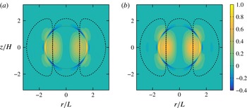
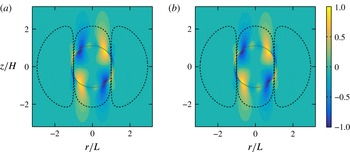
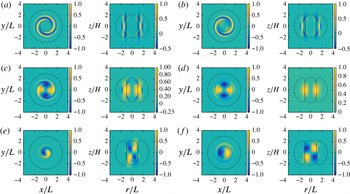
changes from positive to zero.) Figure 2(b) shows that this condition is met. Figure 3 shows the vertical vorticity of the eigenmodes whose eigenvalues are shown in figure 2 with
 $Bu=0.7$
(where the eigenmode is unstable) and
 $Bu=0.9$
(where the eigenmode is neutrally stable). The eigenmodes clearly have similar radial structures and are therefore part of the same family. The continuous, nearly circular curve (dark green, in colour) is the locus in the
 $r{-}z$
plane where
 $v_{\unicode[STIX]{x1D719}}(r,z)/r=c$
and indicates the theoretical location of the critical layer. The large vorticity that is nearly coincident with the continuous curve is the critical layer.
Vertical vorticity in the
 $(r{-}z)$
plane of two of the eigenmodes shown in figure 2, with medium shade being zero (cyan, in colour), light shade being the most cyclonic (yellow, in colour) and dark shade the most anticyclonic (blue, in colour). The centre of each panel corresponds to the centre of the unperturbed Gaussian vortex. The azimuthal angle of each panel was chosen so that the critical layer is prominent. The theoretical location of each critical layer is indicated by the continuous, nearly circular curve (dark green, in colour), which is where the phase speed
 $c$
is equal to the azimuthal velocity of the unperturbed vortex. Both eigenmodes have S2 symmetry. (a) For the unstable eigenmode at
 $Bu=0.7$
. (b) For the neutrally stable eigenmode at
 $Bu=0.9$
. The similarity of the radial structure of the unstable and neutrally stable eigenmodes indicate that they are part of the same family and that the family does not terminate when the growth rate changes from positive to zero.

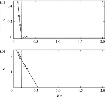
Figures 4 and 5 show the growth rates, phase speeds and the vertical vorticity of another family of eigenmodes with critical layers for
 $Ro=0.05$
and
 $0\leqslant Bu\leqslant 2.1$
. These eigenmodes have A1 symmetry and are the fastest-growing eigenmodes when
 $Bu\lesssim 0.2$
. As
 $Bu$
increases, the growth rate changes from positive (unstable) to zero (neutrally stable) at
 $Bu\simeq 0.177$
. The continuity of
 $c$
and the similarity of the vorticity distributions for the unstable and neutrally stable eigenmodes indicate that the unstable and neutrally stable eigenmodes belong to the same family and that the family does not end abruptly at the value of
 $Bu$
where the eigenmodes pass from unstable to neutrally stable.
As in figure 2 but for the family of A1 eigenmodes that are the fastest growing for
 $Ro=0.05$
,
 $f/\bar{N}=0.1$
and in the range
 $Bu\lesssim 0.2$
. Triangles indicate the numerically computed values of
 $\unicode[STIX]{x1D70E}$
and
 $c$
. The eigenmode goes from unstable to neutrally stable at
 $Bu\simeq 0.177$
, indicated by the vertical broken line.


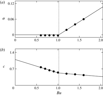
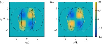
Figures 6 and 7 also show the growth rates and phase speeds and the vertical vorticity of a different family of eigenmodes with critical layers with A1 symmetry for
 $Ro=0.05$
and
 $0\leqslant Bu\leqslant 2.1$
. For this family as
 $Bu$
decreases, the growth rate changes from positive (unstable) to zero (neutrally stable) at
 $Bu\simeq 1.02$
. Again, the continuity of
 $c$
and the similarity of the vorticity distributions for the unstable and neutrally stable eigenmodes indicate that the unstable and neutrally stable eigenmodes belong to the same family and that the family does not end abruptly at the value of
 $Bu$
where the eigenmodes pass from unstable to neutrally stable. Note that although the set of figures 4 and 5 and the set of figures 6 and 7 both illustrate A1 eigenmodes, they are different families of eigenmodes. The distinction is easily seen because the radial structures of the eigenmodes differ and because the phase speeds differ. We have illustrated these two different families of A1 eigenmodes to emphasize the fact that we can easily determine when two families of eigenmodes are distinct and when they are not. These results demonstrate that the unstable and neutrally stable eigenmodes in figure 2 (or in figure 4 or in figure 6) are part of the same family and confirm that when a pair of eigenvalues of eigenmodes of the vortices studied here collide on the imaginary axis, the families of eigenmodes do not terminate. This finding will be used later to interpret the results of § 4 (specifically, figure 9).
Finally, it should be mentioned that for the cases examined here (
 $Ro=0.05$
,
 $0.1\lesssim Bu\lesssim 1.6$
), the peripheral location of critical layers is found to be generic (figures 3, 5, 7 and 14
f), which is consistent with the QG analysis of Nguyen et al. (Reference Nguyen, Hua, Schopp and Carton2012).
As in figure 2 but for the family of A1 eigenmodes that are the fastest growing for
 $Ro=0.05$
,
 $f/\bar{N}=0.1$
, and
 $Bu\gtrsim 1$
. Solid circles indicate the numerically computed values of
 $\unicode[STIX]{x1D70E}$
and
 $c$
. The eigenmode goes from neutrally stable to unstable at
 $Bu\simeq 1.02$
indicated by the vertical broken line. Note that the families illustrated here and in figure 4 both have A1 symmetry, but they are different families.

As in figure 3 but for two of the eigenmodes shown in figure 6 with A1 symmetry. (a) For the unstable eigenmode at
 $Bu=1.2$
. (b) For the neutrally stable eigenmode at
 $Bu=0.9$
. Note that the eigenmodes illustrated here and in figure 5 both have A1 symmetry, but they are different eigenmodes.

4 Parameter map of stability
Here, we explore the stability and linear growth rates of Gaussian vortices as functions of
 $Ro$
and
 $Bu$
for
 $f/\bar{N}=0.1$
. Like many other studies, for most cases we have used
 $f/\bar{N}=0.1$
, rather than
 $f/\bar{N}=0.01$
(which is a better representative of the mid-latitude oceans, see Chelton, deSzoeke & Schlax Reference Chelton, deSzoeke and Schlax1998; Lelong & Sundermeyer Reference Lelong and Sundermeyer2005), because small values of
 $f/\bar{N}$
are computationally expensive to tackle (see, e.g. Brunner-Suzuki et al.
Reference Brunner-Suzuki, Sundermeyer and Lelong2012; Tsang & Dritschel Reference Tsang and Dritschel2015). However in this paper, we use the semi-analytic method of Barranco & Marcus (Reference Barranco and Marcus2006), which allows us to compute flows efficiently for a wide range of
 $f/\bar{N}$
, including the more physically relevant value of 0.01. Some cases are repeated with
 $f/\bar{N}=0.01$
and discussed in § 5. The results presented in this section are all obtained using the computational domain of
 $(30L)\times (30L)\times (30H)$
and resolution of
 $256^{3}$
.
For each of the vortices we examined, we computed the eigenvalues and eigenvectors (as given by (2.10)) of the fastest-growing eigenmode and also for the fastest-growing eigenmodes of each of the six symmetry classes that could be computed by the simultaneous application of the spatial symmetrizer in
 $z$
(which forced the eigenmode to be symmetric or antisymmetric in
 $z$
) and the azimuthal symmetrizer (which forced the eigenmode to have an odd azimuthal wavenumber
 $m$
, or to have an even
 $m$
that was not divisible by 4, or to have an even
 $m$
that was divisible by 4). For some cases, the fastest-growing eigenmodes were also computed without a spatial symmetrizer, which were found to be identical (up to three significant digits) to the fastest-growing eigenmode of the six eigenmodes that were computed with one of the enforced symmetries.
The results are compared and contrasted with the most relevant published results obtained from analysing the QG, shallow-water, and full Boussinesq equations in § 4.2.
4.1 Spatial symmetries and growth rates of the eigenmodes
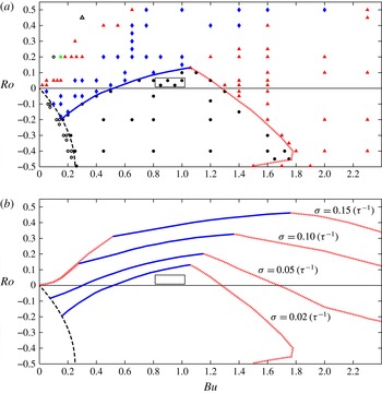
The parameter map of stability in the
 $Ro{-}Bu$
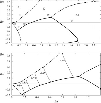
space is shown in figure 8(a). Gaussian anticyclones do not exist with
 $Ro<-0.5$
(see § 2.3). The region to the lower left of the thick dashed black curve corresponds to equilibrium Gaussian vortices for which
 $N_{c}^{2}<0$
(or
 $Bu<-Ro(1+Ro)$
according to (2.7)). These vortices are not unphysical, but near their cores they have heavy fluid above light fluid (i.e.
 $\unicode[STIX]{x2202}\unicode[STIX]{x1D70C}/\unicode[STIX]{x2202}z>0$
at the vortex centre).
As shown in figure 8(a), the most unstable eigenmodes (i.e. those with the largest growth rates) of the vortices generally have either S2 or A1 symmetries. A few points in the figure correspond to vortices for which the fastest-growing eigenmode is A2, A3 or A4. We found that no vortex had a fastest-growing eigenmode with a symmetry different from those just listed. To our surprise, only four out of the 130 vortices that we examined were neutrally stable. All the neutrally stable vortices were cyclones with
 $0.02\lesssim Ro\lesssim 0.05$
and
 $0.8\lesssim Bu\lesssim 1$
. The neutrally stable eigenmodes are denoted in figure 8(a) as solid circles in the region circumscribed by a small rectangle. The rectangle is to ‘guide the eye’ and is used to denote the approximate boundary of the region of neutral stability. Computing the actual boundary between the regions where vortices are all neutrally stable and where they are unstable would be expensive and rather pointless given how small the neutrally stable region is. Anticyclones have linear growth rates that are slow and would not destroy a vortex in less than 50 vortex turnaround times if
 $0.5\lesssim Bu\lesssim 1.3$
. For nearly geostrophic cyclones with
 $|Ro|<0.05$
, linear growth rates are slow and would not destroy a vortex in less than 50 vortex turnaround times if
 $0.7\lesssim Bu\lesssim 1.2$
. As
 $Ro$
increases, the growth rates of large diameter cyclones (i.e. with
 $Bu\lesssim 1.05$
or
 $L\gtrsim 0.98L_{r}$
) becomes faster.
Parameter map of the stability of Gaussian vortices in the
 $Ro{-}Bu$
space. No equilibrium Gaussian vortices exist with
 $Ro<-0.5$
. The thick black dashed line in the lower left corner indicates the locus over which
 $N_{c}^{2}=0$
, i.e.
 $Bu=-Ro(1+Ro)$
, with
 $N_{c}^{2}<0$
for vortices with smaller
 $Ro$
or
 $Bu$
. Panel (a): the thick solid (blue, in colour) and thick dotted (red, in colour) lines indicate the iso-surface where
 $\unicode[STIX]{x1D70E}$
of the fastest-growing eigenmode is
 $0.02\unicode[STIX]{x1D70F}^{-1}$
. The region bounded by this iso-surface, the thick black dashed curve (but see the caveat in the text describing figure 10) and the bottom of the figure has
 $\unicode[STIX]{x1D70E}<0.02\unicode[STIX]{x1D70F}^{-1}$
(the iso-contour is to guide the eye and is approximated by interpolating among the growth rates calculated at the locations of the discrete symbols). The symbols denote the spatial symmetry of the fastest-growing eigenmode, with diamonds (blue, in colour) as S2, solid triangles (red, in colour) as A1, squares (green, in colour) as A2, hollow triangles as A3 and hollow circles as A4. Black solid circles correspond to vortices for which the most unstable eigenmodes have growth rates slower than
 $0.02\unicode[STIX]{x1D70F}^{-1}$
. Panel (b): four iso-contours (approximated as in (a)) of growth rate
 $\unicode[STIX]{x1D70E}$
of the fastest-growing eigenmode. Each contour consists of one solid curve (blue, in colour) and one or two dotted curves (red, in colour). The fastest-growing eigenmodes along the dotted curves (red, in colour) have A1 symmetry and along the solid curves (blue, in colour) have S2 symmetry. The small rectangular box near
 $Bu=1$
is to guide the eye and shows the approximate, very small, region where all of the eigenmodes of the cyclones are neutrally stable. The
 $\unicode[STIX]{x1D70E}$
and the symmetries of the most unstable eigenmodes with
 $\unicode[STIX]{x1D70E}>0.02\unicode[STIX]{x1D70F}^{-1}$
for vortices with
 $N_{c}^{2}>0$
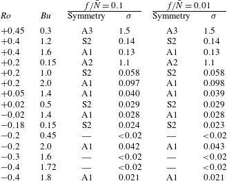
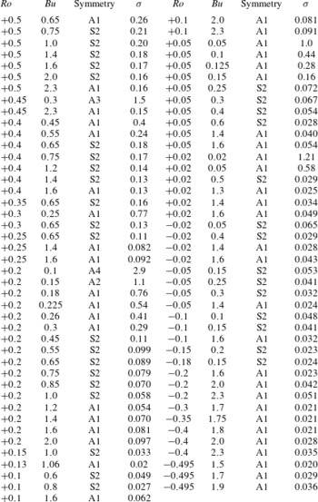
in (a) are given in appendix D.

Considering the smallness of the region of neutral stability, clearly, linear stability cannot be used to explain the differences between the numbers of observed cyclones and anticyclones in the oceans or in planetary atmospheres. On the other hand, ocean vortices can survive for more than 50 of their own turnaround times,
 $\unicode[STIX]{x1D70F}$
. So, one plausible explanation of the cyclonic/anticyclonic asymmetry in the frequency of observation of mesoscale oceanic eddies and of planetary vortices might depend on the differences of the growth rates of the linear instabilities, rather than just the fact that some vortices are not linearly unstable and others are. For example, if there are physical processes (such as turbulence, interactions with other vortices or currents or boundaries) that are likely to destroy a vortex after
 $50\unicode[STIX]{x1D70F}$
, which is more than
 ${\sim}1/2$
year for ocean Meddies (McWilliams Reference McWilliams1985; Armi et al.
Reference Armi, Hebert, Oakey, Price, Richardson, Rossby and Ruddick1989; Hebert, Oakey & Ruddick Reference Hebert, Oakey and Ruddick1990; Pingree & Le Cann Reference Pingree and Le Cann1993; D’Asaro, Walker & Baker Reference D’Asaro, Walker and Baker1994; Prater & Sanford Reference Prater and Sanford1994; Paillet et al.
Reference Paillet, Le Cann, Carton, Morel and Serpette2002), then a vortex need not be neutrally stable to be observed, it needs only have growth rates less than
 ${\sim}1/50\unicode[STIX]{x1D70F}^{-1}$
. So, it is plausible that the asymmetry between the numbers of observed cyclones and anticyclones depends upon the relative amount of area in
 $Ro{-}Bu$
parameter space for which the fastest-growing eigenmodes grow slower than
 ${\sim}1/50\unicode[STIX]{x1D70F}^{-1}$
, or some other critical growth rate. For Gaussian vortices, the region in
 $Ro{-}Bu$
parameter space where the growth rate of the fastest-growing eigenmode is less than
 $1/50\unicode[STIX]{x1D70F}^{-1}$
(i.e. the ‘slow growth region’ for linear instability) is the region bounded above by the solid (blue, in colour) and dotted (red, in colour) curves in figure 8(a) and to the lower left by the thick dashed curve. Along the solid curve (blue, in colour), the fastest-growing eigenmode has S2 symmetry, whereas along the dotted curve (red, in colour) it is A1. The solid and dotted curves are drawn to guide the eye, and the vortices corresponding to the black solid circles have
 $\unicode[STIX]{x1D70E}<1/50\unicode[STIX]{x1D70F}^{-1}$
. In general, for large
 $Bu$
, the fastest-growing eigenmodes have A1 symmetry, while for smaller
 $Bu$
, they have S2 symmetry. However, for cyclones with
 $Bu\lesssim 0.4$
, some of the fastest-growing eigenmodes also have A1 symmetry, or even A2, A3 or A4 symmetry, and the growth rates are often faster than
 $1\unicode[STIX]{x1D70F}^{-1}$
. There are two regions in the
 $Ro{-}Bu$
parameter space where the fastest-growing eigenmodes of the cyclones have A1 symmetry. In the region with higher
 $Bu$
, the growth rate of the fastest-growing modes is smaller than that in the lower
 $Bu$
region, and, as discussed previously and elaborated on in § 6, the radial structures of the fastest-growing A1 eigenmodes in the large and small
 $Bu$
regions differ as well.
Of course, our choice of
 $50\unicode[STIX]{x1D70F}$
to define the ‘slow growth region’ for linear instability is arbitrary, so figure 8(b) shows how the slow growth region changes when we change our choice from
 $50\unicode[STIX]{x1D70F}$
to
 $20\unicode[STIX]{x1D70F}$
,
 $10\unicode[STIX]{x1D70F}$
or
 $6.67\unicode[STIX]{x1D70F}$
. That is, the two sets of (solid/broken) curves are iso-surfaces in
 $Ro{-}Bu$
parameter space where
 $\unicode[STIX]{x1D70E}$
is 0.02, 0.05, 0.1 and 0.15 in units of
 $\unicode[STIX]{x1D70F}^{-1}$
. For the iso-surface for the growth rate of
 $0.15\unicode[STIX]{x1D70F}^{-1}$
in figure 8(b), the fastest-growing eigenmode has S2 symmetry for
 $0.5\lesssim Bu\lesssim 1.8$
, otherwise the fastest-growing eigenmode has A1 symmetry. Note that the iso-surfaces for the growth rates of
 $0.10\unicode[STIX]{x1D70F}^{-1}$
and
 $0.15\unicode[STIX]{x1D70F}^{-1}$
are very close to each other for
 $Bu\lesssim 0.3$
. Most of the fastest-growing eigenmodes in the
 $Ro{-}Bu$
parameter space shown in figure 8 have
 $\unicode[STIX]{x1D70E}<0.2\unicode[STIX]{x1D70F}^{-1}$
. However, cyclones in the upper left corner of figure 8 can have
 $\unicode[STIX]{x1D70E}$
of order one
 $\unicode[STIX]{x1D70F}^{-1}$
. As shown below, anticyclones to the lower left of the thick dashed curve in the lower left side of figure 8 (with
 $N_{c}^{2}<0$
) can have much larger
 $\unicode[STIX]{x1D70E}$
.
The growth rates of the three fastest-growing eigenmodes for
 $Ro=0.05$
as functions of
 $Bu$
are plotted in figure 9(a) (combining figures 2, 4 and 6) showing that the fastest-growing eigenmode is A1 for
 $Bu\lesssim 0.2$
; is S2 for
 $0.2\lesssim Bu\lesssim 0.8$
; and is A1 for
 $1\lesssim Bu\lesssim 2.1$
. However, for
 $0.8\lesssim Bu\lesssim 1$
, the eigenmodes are all neutrally stable. This region of neutral stability is consistent with the neutrally stable region shown in figure 8. The change in the spatial symmetry from A1 to S2 back to A1 of the fastest-growing eigenmode as
 $Bu$
increases was discussed in § 3 and it was shown that (i) the family of eigenmodes continues to exist even after the eigenmodes become neutrally stable and (ii) the A1 modes at small and large
 $Bu$
belong to two different families of eigenmodes. Similar changes in the symmetries of the most unstable mode are observed at
 $Ro=0.2$
(figure 9
b); however, at
 $Ro=0.2$
there is not a region where the vortex is neutrally stable to all eigenmodes. Similar to
 $Ro=0.05$
, the two families of A1 eigenmodes shown in figure 9(b) with triangles and with filled circles are distinct families with different radial structures. How these results, particularly at the small
 $Ro$
of 0.05, compare with those obtained from analysing the QG equations is discussed in § 4.2.
Growth rates
 $\unicode[STIX]{x1D70E}$
(in units of
 $\unicode[STIX]{x1D70F}^{-1}$
) of the three fastest-growing modes as functions of
 $Bu$
for fixed
 $Ro$
.
 $f/\bar{N}=0.1$
. Triangles, filled circles and diamonds, respectively, indicate the fastest-growing eigenmodes at low
 $Bu$
(which have A1 symmetry), the fastest-growing eigenmodes at high
 $Bu$
(which also have A1 symmetry) and the fastest-growing eigenmodes for intermediate
 $Bu$
(which have S2 symmetry). The three lines connecting the three sets of symbols are to guide the eye to show the three families of eigenmodes. (a)
 $Ro=0.05$
; in this case as
 $Bu$
increases, the fastest-growing mode changes from A1 to S2; then all modes are linearly neutrally stable; then the fastest-growing mode is A1. (b)
 $Ro=0.2$
; the fastest-growing mode changes from A1 to S2 and again to A1 as
 $Bu$
increases.

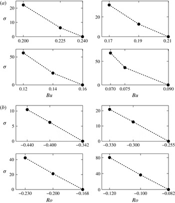
The growth rates for the region with statically unstable vortex cores, i.e. with
 $N_{c}^{2}<0$
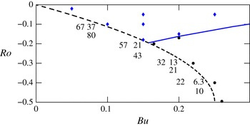
, are shown in figure 10. Eigenmodes for this region have A4 symmetry and the growth rates can be as large as
 ${\sim}100\unicode[STIX]{x1D70F}^{-1}$
. The
 $\unicode[STIX]{x1D70E}$
as a function of
 $Bu$
(for fixed
 $Ro$
), and as a function of
 $Ro$
(for fixed
 $Bu$
) for vortices with
 $N_{c}^{2}<0$
are shown in figures 11(a) and 11(b), respectively. In each of the eight panels, the value of the horizontal coordinate axis on the right-hand side of the panel corresponds to a vortex with
 $N_{c}^{2}=0$
(i.e. a point on the thick dashed curve in figure 8 or in the broken curve in figure 10). The figure shows that
 $\unicode[STIX]{x1D70E}$
increases rapidly as a function of distance from the
 $N_{c}^{2}=0$
boundary. Due to this rapid growth in
 $\unicode[STIX]{x1D70E}$
, for all practical purposes we can consider the thick dashed line at
 $N_{c}^{2}=0$
to be the left boundary of the region in figure 8(b) in
 $Ro{-}Bu$
for which
 $\unicode[STIX]{x1D70E}<0.02\unicode[STIX]{x1D70F}^{-1}$
, and also the boundary for the region
 $0.02\unicode[STIX]{x1D70F}^{-1}\leqslant \unicode[STIX]{x1D70E}<0.05\unicode[STIX]{x1D70F}^{-1}$
, and for the region
 $0.05\unicode[STIX]{x1D70F}^{-1}\leqslant \unicode[STIX]{x1D70E}<0.10\unicode[STIX]{x1D70F}^{-1}$
.
Blow up of the lower left corner of figure 8(a), showing details of the eigenvalues in the region where the Gaussian vortices have
 $N_{c}^{2}<0$
. The axes of the figure, line styles and symbols have the same meaning as they do in figure 8(a). In the lower left region, below the broken line, numbers rather than symbols are used to indicate where in parameter space we have carried out linear stability calculations. The numbers are the values
 $\unicode[STIX]{x1D70E}$
(in units of
 $\unicode[STIX]{x1D70F}^{-1}$
) of the fastest-growing eigenmode (which in all cases has an A4 symmetry).

Growth rates (in units of
 $\unicode[STIX]{x1D70F}^{-1}$
) for the most unstable eigenmode of vortices with
 $N_{c}^{2}<0$
for fixed
 $Ro$
and
 $Bu$
.
 $f/\bar{N}=0.1$
. For all vortices examined in this region, the fastest-growing eigenmode has A4 symmetry; (a)
 $\unicode[STIX]{x1D70E}$
as a function of
 $Bu$
for
 $Ro=-0.4$
,
 $-0.3$
,
 $-0.2$
and
 $-0.1$
; (b)
 $\unicode[STIX]{x1D70E}$
as a function of
 $Ro$
for
 $Bu=0.225$
, 0.19, 0.14 and 0.075. In each panel, the value of the horizontal coordinate axis on the right side of the panel corresponds to a vortex with
 $N_{c}^{2}=0$
. The dotted lines are to guide the eye.

4.2 Comparison with previous studies
As discussed in § 1, this paper extends the analyses of previous studies by using the full 3-D non-hydrostatic Boussinesq equations and by employing the 3-D Gaussian vortex model, which has continuous velocity and density (and PV) fields and is initially in exact equilibrium. The latter is necessary for a rigorous linear stability analysis. A comparison of our results with those of many previous studies is not straightforward because various different vortex models and flow models have been used. Below we compare our parameter map of stability with the results of the most relevant study in the QG limit (Nguyen et al. Reference Nguyen, Hua, Schopp and Carton2012) and with the results of several relevant studies using multilayer models. We also discuss the results of Yim et al. (Reference Yim, Billant and Ménesguen2016), who used the full Boussinesq equations but studied a different family of vortices.
In the limit of vanishing
 $Ro$
, the most relevant study to ours is that of Nguyen et al. (Reference Nguyen, Hua, Schopp and Carton2012), who numerically calculated the unstable modes of a Gaussian vortex using the QG equations. They found that the fastest-growing mode changes from S2 to A1 around
 $Bu=1$
, which along with the general dependence of the growth rate of the fastest-growing mode on
 $Bu$
in their figure 1(a) agrees overall with the results of current study (see figure 9
a which is for
 $Ro=0.05$
). However, they also found that for
 $Bu$
as small as 0.05, modes with higher
 $m$
dominate. In our results, for anticyclones, as
 $Bu$
decreases, the most unstable mode changes from S2 to A4 once the vortex becomes statically unstable (this instability is not considered in the QG framework used by Nguyen et al. (Reference Nguyen, Hua, Schopp and Carton2012)). For cyclones, as
 $Bu$
decreases, the most unstable mode changes from S2 to A1 for small
 $Ro$
and to A2 or A3 for moderate
 $Ro$
(see figure 8).
There are a number of studies which have used the shallow-water equations with the Gaussian vortex model and are relevant to current work. Consistent with the results of our analysis, these studies find that anticyclones become more stable as the absolute value of the Rossby number increases, whereas for cyclones the growth rates decrease with decreasing the Rossby number (Stegner & Dritschel Reference Stegner and Dritschel2000; Baey & Carton Reference Baey and Carton2002; Benilov & Flanagan Reference Benilov and Flanagan2008). (In this section note that our results are only for vortices with stably stratified interiors.)
How the growth rates in these studies vary with the Burger number, however, shows a strong dependence on the vertical structure of the vortex and the background flow. Stegner & Dritschel (Reference Stegner and Dritschel2000) studied the stability of isolated Gaussian vortices using a
 $1{-}1/2$
layer model and found that for vortices with small Rossby numbers, the growth rate decreases with decreasing the Burger number. This is consistent with our results only for
 $Bu\gtrsim 1$
. Benilov & Flanagan (Reference Benilov and Flanagan2008) used a two-layer model to examine the stability of the ‘compensated’ (i.e.
 $\boldsymbol{v}=\mathbf{0}$
in the bottom layer) Gaussian vortices, and also Gaussian vortices with uniform PV in the lower layer. They found that compensated vortices are neutrally stable for intermediate Burger numbers, while vortices with uniform PV in the lower layer are neutrally stable for Burger numbers smaller than a critical value of order 1. Baey & Carton (Reference Baey and Carton2002) studied two-layer Gaussian vortices and found, in contrast to the previous results and those of ours, that the growth rate decreases with Burger number for both cyclones and anticyclones and the eigenmodes are stable for Burger numbers larger than a critical value. It is apparent that identifying a unique stability behaviour with Burger number in these studies is difficult and the behaviour is highly dependent on the vertical structure of the flow/vortex. An example of such dependence is given by Sutyrin (Reference Sutyrin2015), who examined two- and three-layer compensated shallow-water vortices and showed that the addition of a third middle layer with uniform PV weakens the coupling between the upper and lower layers and enhances the stability of vortices. Considering these results, comparing the Burger number dependence of the stability behaviour of 3-D vortices in continuously stratified Boussinesq flows and vortices in shallow water and layer models is not particularly useful.
Only a few studies have used the full Boussinesq equations, and even those have focused on very different vortex models such as barotropic Taylor columns (Smyth & McWilliams Reference Smyth and McWilliams1998), evolving (out-of-equilibrium) 3-D vortices interacting with large-scale internal waves (Brunner-Suzuki et al. Reference Brunner-Suzuki, Sundermeyer and Lelong2012), out-of-equilibrium, ellipsoidal 3-D vortices with discontinuous PV profiles (Tsang & Dritschel Reference Tsang and Dritschel2015) and 3-D equilibrium vortices with Gaussian angular velocity (Yim et al. Reference Yim, Billant and Ménesguen2016). Here we focus on the latter, because the main difference between our analysis and that of Yim et al. (Reference Yim, Billant and Ménesguen2016) is in the vortex model: Gaussian pressure anomaly in the current study versus their Gaussian angular velocity (also note that the flow in their study is not inviscid). Such comparison provides some understanding of how the stability properties depend on the vortex profile.
Yim et al. (Reference Yim, Billant and Ménesguen2016) conducted a linear stability analysis of 3-D equilibrium vortices with Gaussian angular velocity in unbounded, rotating, stratified flows for a wide range of Rossby numbers,
 $|Ro|\leqslant 20$
. Here we only focus on their results for
 $|Ro|\leqslant 0.5$
and inviscid and non-diffusive flows, which are relevant to the present study. Consistent with our results, for
 $Bu\gtrsim 1$
, they found A1 as the most unstable mode for both cyclones and anticyclones (their figure 39d and f), which they attributed to the instability mechanism of Gent & McWilliams (Reference Gent and McWilliams1986) (this is also consistent with the results of Smyth & McWilliams (Reference Smyth and McWilliams1998) for Taylor columns). For
 $Bu\lesssim 1$
, Yim et al. (Reference Yim, Billant and Ménesguen2016) found anticyclones neutrally stable for
 $0.5\lesssim Bu\lesssim 1$
(while we found them weakly unstable), and they found S2 as the most unstable mode for anticyclones between the statically unstable region and
 $Bu\sim 0.4{-}0.5$
(depending on
 $Ro$
), which is consistent with our results. For cyclones with
 $Bu\lesssim 1$
, Yim et al. (Reference Yim, Billant and Ménesguen2016) found a neutrally stable region between
 $0.5\lesssim Bu\lesssim 1$
(variable with
 $Ro$
), which is much larger than (and encompasses) the neutrally stable region we found; they also found that as
 $Bu$
decreases from one, modes with
 $m=2$
become the most unstable ones before modes with
 $m=1$
also becoming unstable at lower
 $Bu$
, which is overall consistent with our results. At
 $Bu$
as low as 0.3, the family of vortices studied by Yim et al. (Reference Yim, Billant and Ménesguen2016) can have statically unstable cyclones, while cyclones in the family of vortices we studied are always statically stable. The comparison of the results of the current study and those of Yim et al. (Reference Yim, Billant and Ménesguen2016), as summarized above, suggests that for these two vortex families, while the linear stability properties are not sensitive to the vortex profile for
 $Bu\gtrsim 1$
, the stability properties strongly depend on the vortex profile for
 $Bu\lesssim 1$
. Whether this behaviour is generic or not requires further studies with other vortex families.
5 Effect of
$f/\bar{N}$
on linear stability

Despite the fact that
 $f/\bar{N}$
is of order 0.01 in the mid-latitude oceans (Chelton et al.
Reference Chelton, deSzoeke and Schlax1998; Sundermeyer & Lelong Reference Sundermeyer and Lelong2005),
 $f/\bar{N}\sim 0.1$
is commonly used in studies of the oceanic vortices to reduce the computational cost; small values of
 $f/\bar{N}$
in explicit codes makes the equations of motion numerically ‘stiff’, which means they must be computed with small time steps. In this paper calculations are done with
 $f/\bar{N}=0.1$
for the purpose of sweeping a large region of the
 $Ro{-}Bu$
parameter space and comparing our results with those of others who have used this value.
Several other studies (Smyth & McWilliams Reference Smyth and McWilliams1998; Sundermeyer & Lelong Reference Sundermeyer and Lelong2005; Brunner-Suzuki et al.
Reference Brunner-Suzuki, Sundermeyer and Lelong2012; Dritschel & Mckiver Reference Dritschel and Mckiver2015; Tsang & Dritschel Reference Tsang and Dritschel2015) have shown numerically that the stability properties and some aspects of the dynamics of vortices in rotating, stratified flows are not very sensitive to the specific value of
 $f/\bar{N}$
as long as this value is small. Here, we show numerically that the eigenvectors and eigenvalues of Gaussian vortices (with
 $N_{c}^{2}>0$
), when properly scaled, are nearly independent of
 $f/\bar{N}$
for small
 $f/\bar{N}$
. Furthermore, by properly non-dimensionalizing the linearized equations of motion, we explain the insensitivity of the eigenvalues and eigenvector structures of the fastest-growing modes to the value of
 $f/\bar{N}$
.
Exploiting our semi-analytic method that enables us to accurately and efficiently deal with large
 $f\unicode[STIX]{x0394}t$
and
 $\bar{N}\unicode[STIX]{x0394}t$
, we have repeated over 40 of the simulations with
 $f/\bar{N}=0.01$
. Table 1 shows the linear growth rate and the spatial symmetry of the fastest-growing eigenmode of several Gaussian vortices for
 $f/\bar{N}=0.1$
and
 $f/\bar{N}=0.01$
. The symmetries are the same in all cases, as are the growth rates (in units of
 $\unicode[STIX]{x1D70F}^{-1}$
) within 4 %. Figure 12 shows examples of the most unstable eigenvectors (with dimension in
 $z$
scaled by
 $H$
and dimensions of
 $r$
,
 $x$
and
 $y$
scaled by
 $L$
). The eigenmodes are nearly indistinguishable for
 $f/\bar{N}=0.1$
and
 $f/\bar{N}=0.01$
.
Comparison of the linear growth rates (in units of
 $\unicode[STIX]{x1D70F}^{-1}$
) and symmetries of the most unstable eigenmode of selected Gaussian vortices in the
 $Ro{-}Bu$
space for
 $f/\bar{N}=0.1$
and
 $f/\bar{N}=0.01$
.
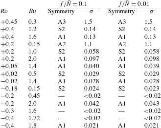
The insensitivity to
 $f/\bar{N}$
is easily explained by non-dimensionalizing the equations of motion (2.1) with
 $4\unicode[STIX]{x03C0}/\unicode[STIX]{x1D714}_{c}\equiv \unicode[STIX]{x1D70F}$
as the unit of time,
 $L$
as the unit of horizontal length,
 $H$
as the unit of vertical length,
 $L/\unicode[STIX]{x1D70F}$
as the unit of horizontal velocity,
 $H/\unicode[STIX]{x1D70F}$
as the unit of vertical velocity,
 $\unicode[STIX]{x1D70C}_{o}fL^{2}/\unicode[STIX]{x1D70F}$
as the unit of pressure,
 $\unicode[STIX]{x1D70C}_{o}$
as the unit of density and
 $fL^{2}/(H\unicode[STIX]{x1D70F})$
as the unit of buoyancy. In the following equations, asterisk superscripts indicate the non-dimensionalized quantity or operator
 $$\begin{eqnarray}\displaystyle & \displaystyle \left(\frac{Ro}{2\unicode[STIX]{x03C0}}\right)\left[\frac{\unicode[STIX]{x2202}v_{r}^{\ast }}{\unicode[STIX]{x2202}t^{\ast }}+v_{r}^{\ast }\frac{\unicode[STIX]{x2202}v_{r}^{\ast }}{\unicode[STIX]{x2202}r^{\ast }}+\frac{v_{\unicode[STIX]{x1D719}}^{\ast }}{r^{\ast }}\frac{\unicode[STIX]{x2202}v_{r}^{\ast }}{\unicode[STIX]{x2202}\unicode[STIX]{x1D719}}+v_{z}^{\ast }\frac{\unicode[STIX]{x2202}v_{r}^{\ast }}{\unicode[STIX]{x2202}z^{\ast }}-\frac{{v^{\ast }}_{\unicode[STIX]{x1D719}}^{2}}{r^{\ast }}\right]=-\frac{\unicode[STIX]{x2202}p^{\ast }}{\unicode[STIX]{x2202}r^{\ast }}+v_{\unicode[STIX]{x1D719}}^{\ast }, & \displaystyle\end{eqnarray}$$
 $$\begin{eqnarray}\displaystyle & \displaystyle \left(\frac{Ro}{2\unicode[STIX]{x03C0}}\right)\left[\frac{\unicode[STIX]{x2202}v_{\unicode[STIX]{x1D719}}^{\ast }}{\unicode[STIX]{x2202}t^{\ast }}+v_{r}^{\ast }\frac{\unicode[STIX]{x2202}v_{\unicode[STIX]{x1D719}}^{\ast }}{\unicode[STIX]{x2202}r^{\ast }}+\frac{v_{\unicode[STIX]{x1D719}}^{\ast }}{r^{\ast }}\frac{\unicode[STIX]{x2202}v_{\unicode[STIX]{x1D719}}^{\ast }}{\unicode[STIX]{x2202}\unicode[STIX]{x1D719}}+v_{z}^{\ast }\frac{\unicode[STIX]{x2202}v_{\unicode[STIX]{x1D719}}^{\ast }}{\unicode[STIX]{x2202}z^{\ast }}+\frac{v_{r}^{\ast }v_{\unicode[STIX]{x1D719}}^{\ast }}{r^{\ast }}\right]=-\frac{1}{r^{\ast }}\frac{\unicode[STIX]{x2202}p^{\ast }}{\unicode[STIX]{x2202}\unicode[STIX]{x1D719}}-v_{r}^{\ast }, & \displaystyle\end{eqnarray}$$
 $$\begin{eqnarray}\displaystyle & \displaystyle \left(\frac{Ro}{2\unicode[STIX]{x03C0}}\right)(Bu)\left(\frac{f}{\bar{N}}\right)^{2}\left[\frac{\unicode[STIX]{x2202}v_{z}^{\ast }}{\unicode[STIX]{x2202}t^{\ast }}+v_{r}^{\ast }\frac{\unicode[STIX]{x2202}v_{z}^{\ast }}{\unicode[STIX]{x2202}r^{\ast }}+\frac{v_{\unicode[STIX]{x1D719}}^{\ast }}{r^{\ast }}\frac{\unicode[STIX]{x2202}v_{z}^{\ast }}{\unicode[STIX]{x2202}\unicode[STIX]{x1D719}}+v_{z}^{\ast }\frac{\unicode[STIX]{x2202}v_{z}^{\ast }}{\unicode[STIX]{x2202}z^{\ast }}\right]=-\frac{\unicode[STIX]{x2202}p^{\ast }}{\unicode[STIX]{x2202}z^{\ast }}+b^{\ast }, & \displaystyle\end{eqnarray}$$
 $$\begin{eqnarray}\displaystyle & \displaystyle \left(\frac{Ro}{2\unicode[STIX]{x03C0}Bu}\right)\left[\frac{\unicode[STIX]{x2202}b^{\ast }}{\unicode[STIX]{x2202}t^{\ast }}+v_{r}^{\ast }\frac{\unicode[STIX]{x2202}b^{\ast }}{\unicode[STIX]{x2202}r^{\ast }}+\frac{v_{\unicode[STIX]{x1D719}}^{\ast }}{r^{\ast }}\frac{\unicode[STIX]{x2202}b^{\ast }}{\unicode[STIX]{x2202}\unicode[STIX]{x1D719}}+v_{z}^{\ast }\frac{\unicode[STIX]{x2202}b^{\ast }}{\unicode[STIX]{x2202}z^{\ast }}\right]=-v_{z}^{\ast }, & \displaystyle\end{eqnarray}$$
 $$\begin{eqnarray}\displaystyle & \displaystyle \frac{v_{r}^{\ast }}{r^{\ast }}+\frac{\unicode[STIX]{x2202}v_{r}^{\ast }}{\unicode[STIX]{x2202}r^{\ast }}+\frac{1}{r^{\ast }}\frac{\unicode[STIX]{x2202}v_{\unicode[STIX]{x1D719}}^{\ast }}{\unicode[STIX]{x2202}\unicode[STIX]{x1D719}}+\frac{\unicode[STIX]{x2202}v_{z}^{\ast }}{\unicode[STIX]{x2202}z^{\ast }}=0. & \displaystyle\end{eqnarray}$$
Only (5.3) depends on
 $f/\bar{N}$
. For
 $f/\bar{N}\leqslant 0.1$
and for Burger numbers of order unity or less, the left-hand side of (5.3) is of order
 $10^{-3}$
, whereas the two terms on the right-hand side are both of order unity if we have chosen ‘proper’ units of length, time and mass in our non-dimensionalization such that the dimensionless quantities denoted with asterisk superscripts and their derivatives with respect to the dimensionless length and time inside the square brackets are of order unity or less. Thus those two terms nearly cancel each other, or
 $$\begin{eqnarray}\frac{\unicode[STIX]{x2202}p^{\ast }}{\unicode[STIX]{x2202}z^{\ast }}=b^{\ast }+O(10^{-3}).\end{eqnarray}$$
So, hydrostatic equilibrium is enforced to one part in a thousand. Thus, replacing the dynamic equation (5.3) with the kinematic equation (5.6) is a very good approximation, and with the replacement, the equations of motion are formally independent of
 $f/\bar{N}$
. However, the argument above is not particularly useful because there is no a priori way of knowing that we chose ‘proper’ units, and, in fact, for many types of waves, with this choice of units, the dimensionless expressions inside the square brackets are much greater than unity, and the waves are not in hydrostatic balance and the value of
 $f/\bar{N}$
is important.
Vertical vorticity of eigenmodes normalized such that the maximum value of
 $|\unicode[STIX]{x1D714}|$
is 1. The eigenmodes are virtually indistinguishable for
 $f/\bar{N}=0.1$
and
 $f/\bar{N}=0.01$
. The four rows from top to bottom correspond to the first four rows in table 1. The broken lines denote the boundaries of the core and shield of the unperturbed Gaussian vortex. Panels (a,b,e,f,i,j,m,n) are for
 $f/\bar{N}=0.1$
and (c,d,g,h,k,l,o,p) are for
 $f/\bar{N}=0.01$
. Panels (a,c,e,g,i,k,m,o) show the eigenmodes in the
 $x$
–
 $y$
plane for a fixed
 $z$
. For the
 $z$
-symmetric eigenmode in the second row, this fixed value is
 $z=0$
. For the antisymmetric eigenmodes in rows 1, 3 and 4, the fixed value of
 $z$
is the positive value of
 $z$
at which
 $|\unicode[STIX]{x1D714}|$
of the eigenmode obtains its maximum value. Panels (b,d,f,h,j,l,n,p) show the eigenmodes in the
 $r$
–
 $z$
plane for fixed azimuthal angle
 $\unicode[STIX]{x1D719}$
. In all cases,
 $\unicode[STIX]{x1D719}$
is chosen so that it is the angle at which
 $\unicode[STIX]{x1D714}$
of the eigenmode obtains its maximum value.

However, with the choice of units above, the dimensionless form of our initial Gaussian equilibrium vortices is
 $$\begin{eqnarray}\displaystyle & \displaystyle \hat{p}^{\ast }=(-\unicode[STIX]{x03C0})(1+Ro)\unicode[STIX]{x1D712}^{\ast }(r^{\ast },z^{\ast }), & \displaystyle\end{eqnarray}$$
 $$\begin{eqnarray}\displaystyle & \displaystyle \hat{v}_{\unicode[STIX]{x1D719}}^{\ast }=\left(\frac{\unicode[STIX]{x03C0}}{Ro}\right)(r^{\ast })\left(-1+\sqrt{1+4Ro(1+Ro)\unicode[STIX]{x1D712}^{\ast }(r^{\ast },z^{\ast })}\right),\quad \hat{v}_{r}^{\ast }=\hat{v}_{z}^{\ast }=0, & \displaystyle\end{eqnarray}$$
 $$\begin{eqnarray}\displaystyle & \displaystyle \hat{b}^{\ast }=(2\unicode[STIX]{x03C0})(1+Ro)z^{\ast }\unicode[STIX]{x1D712}^{\ast }(r^{\ast },z^{\ast }), & \displaystyle\end{eqnarray}$$
where
 $\unicode[STIX]{x1D712}^{\ast }\equiv \exp [-(r^{\ast })^{2}-(z^{\ast })^{2}]$
. Note that the vortices depend on
 $Ro$
, but not on
 $f/\bar{N}$
or
 $Bu$
. Also note that as
 $Ro\rightarrow 0$
, the equilibrium velocity
 $\hat{v}_{\unicode[STIX]{x1D719}}^{\ast }\rightarrow 2\unicode[STIX]{x03C0}r^{\ast }\unicode[STIX]{x1D712}^{\ast }(r^{\ast },z^{\ast })$
and remains of order unity or less. The equilibrium
 $p^{\ast }$
and
 $b^{\ast }$
are also of order unity or less for
 $|Ro|$
of order unity or less.
The non-dimensional equations linearized around the non-dimensional Gaussian vortex are (after dropping the asterisk superscripts and writing
 $\boldsymbol{v}=\hat{\boldsymbol{v}}+\tilde{\boldsymbol{v}}$
,
 $p=\hat{p}+\tilde{p}$
, and
 $b=\hat{b}+\tilde{b}$
, where tilde denotes the linear eigenmode)
 $$\begin{eqnarray}\displaystyle & \displaystyle \left(\frac{Ro}{2\unicode[STIX]{x03C0}}\right)\left[\frac{\unicode[STIX]{x2202}\tilde{v}_{r}}{\unicode[STIX]{x2202}t}+\left(\frac{\hat{v}_{\unicode[STIX]{x1D719}}}{r}\right)\frac{\unicode[STIX]{x2202}\tilde{v}_{r}}{\unicode[STIX]{x2202}\unicode[STIX]{x1D719}}-\left(\frac{2\hat{v}_{\unicode[STIX]{x1D719}}\tilde{v}_{\unicode[STIX]{x1D719}}}{r}\right)\right]=-\frac{\unicode[STIX]{x2202}\tilde{p}}{\unicode[STIX]{x2202}r}+\tilde{v}_{\unicode[STIX]{x1D719}}, & \displaystyle\end{eqnarray}$$
 $$\begin{eqnarray}\displaystyle & \displaystyle \left(\frac{Ro}{2\unicode[STIX]{x03C0}}\right)\!\!\left[\frac{\unicode[STIX]{x2202}\tilde{v}_{\unicode[STIX]{x1D719}}}{\unicode[STIX]{x2202}t}+\left(\frac{\hat{v}_{\unicode[STIX]{x1D719}}}{r}\right)\frac{\unicode[STIX]{x2202}\tilde{v}_{\unicode[STIX]{x1D719}}}{\unicode[STIX]{x2202}\unicode[STIX]{x1D719}}+\left(\frac{\unicode[STIX]{x2202}\hat{v}_{\unicode[STIX]{x1D719}}}{\unicode[STIX]{x2202}r}\right)\tilde{v}_{r}+\left(\frac{\unicode[STIX]{x2202}\hat{v}_{\unicode[STIX]{x1D719}}}{\unicode[STIX]{x2202}z}\right)\tilde{v}_{z}+\left(\frac{\hat{v}_{\unicode[STIX]{x1D719}}}{r}\right)\tilde{v}_{r}\right]=-\frac{1}{r}\frac{\unicode[STIX]{x2202}\tilde{p}}{\unicode[STIX]{x2202}\unicode[STIX]{x1D719}}-\tilde{v}_{r},\;\, & \displaystyle\end{eqnarray}$$
 $$\begin{eqnarray}\displaystyle & \displaystyle (Ro)(Bu)\left(\frac{f}{\bar{N}}\right)^{2}\left(\frac{1}{2\unicode[STIX]{x03C0}}\right)\left[\frac{\unicode[STIX]{x2202}\tilde{v}_{z}}{\unicode[STIX]{x2202}t}+\left(\frac{\hat{v}_{\unicode[STIX]{x1D719}}}{r}\right)\frac{\unicode[STIX]{x2202}\tilde{v}_{z}}{\unicode[STIX]{x2202}\unicode[STIX]{x1D719}}\right]=-\frac{\unicode[STIX]{x2202}\tilde{p}}{\unicode[STIX]{x2202}z}+\tilde{b}, & \displaystyle\end{eqnarray}$$
 $$\begin{eqnarray}\displaystyle & \displaystyle \left(\frac{Ro}{2\unicode[STIX]{x03C0}Bu}\right)\left[\frac{\unicode[STIX]{x2202}\tilde{b}}{\unicode[STIX]{x2202}t}+\left(\frac{\hat{v}_{\unicode[STIX]{x1D719}}}{r}\right)\frac{\unicode[STIX]{x2202}\tilde{b}}{\unicode[STIX]{x2202}\unicode[STIX]{x1D719}}+\left(\frac{\unicode[STIX]{x2202}\hat{b}}{\unicode[STIX]{x2202}r}\right)\tilde{v}_{r}+\left(\frac{\unicode[STIX]{x2202}\hat{b}}{\unicode[STIX]{x2202}z}\right)\tilde{v}_{z}\right]=-\tilde{v}_{z}, & \displaystyle\end{eqnarray}$$
 $$\begin{eqnarray}\displaystyle & \displaystyle \frac{\tilde{v}_{r}}{r}+\frac{\unicode[STIX]{x2202}\tilde{v}_{r}}{\unicode[STIX]{x2202}r}+\frac{1}{r}\frac{\unicode[STIX]{x2202}\tilde{v}_{\unicode[STIX]{x1D719}}}{\unicode[STIX]{x2202}\unicode[STIX]{x1D719}}+\frac{\unicode[STIX]{x2202}\tilde{v}_{z}}{\unicode[STIX]{x2202}z}=0. & \displaystyle\end{eqnarray}$$
For the fastest-growing eigenmodes of vortices with
 $N_{c}^{2}>0$
, we have numerically computed the dimensionless values of the quantities inside the square brackets and found them to be of order unity or less for all of the eigenmodes represented in figure 8. This calculation shows that for vortices whose interior is statically stable, the fastest-growing eigenmodes are in vertical hydrostatic balance and therefore explains why the non-dimensionalized eigenvalues and eigenmodes are insensitive to the value of
 $f/\bar{N}$
for
 $f/\bar{N}\lesssim 0.1$
. It should be emphasized that we could not assume a priori that the fastest-growing eigenmodes of our vortices are in hydrostatic balance. Here we have numerically tested and verified the validity of this assumption. It is worth mentioning that non-hydrostatic effects can be important in the dynamics and evolution of some geophysical and astrophysical vortices; for example, our previous calculations of vortices (Marcus & Hassanzadeh Reference Marcus and Hassanzadeh2014), especially the longevity of the Great Red Spot (GRS) of Jupiter (and we remind the reader that longevity of vortices was the motivation of the study), showed that small departures from vertical hydrostatic equilibrium caused large changes to the lifetime of the GRS (albeit, due to nonlinear effects).
Finally, it is not surprising that for vortices with statically unstable interiors (
 $N_{c}^{2}<0$
), the terms in the square brackets are large and therefore the most unstable eigenmodes are not in hydrostatic balance. We have not carried out further eigenmode calculations with
 $f/\bar{N}=0.01$
in this region because they are computationally very expensive.
6 Radial and vertical structure of the unstable eigenmodes
In this section we investigate the radial distribution of vorticity in the fastest-growing eigenmodes. The spatial distribution of these eigenmodes can be characterized quantitatively by determining the fractional amounts of its vertical enstrophy that are within the Gaussian vortex’s core
 $S_{core}$
and within its shield
 $S_{shield}$
, where we use the definitions of core and shield given in appendix B:
 $$\begin{eqnarray}\displaystyle & \displaystyle S_{core}\equiv \frac{\displaystyle \int _{core}|\unicode[STIX]{x1D714}_{eig}|^{2}\,\text{d}^{3}x}{\displaystyle \int |\unicode[STIX]{x1D714}_{eig}|^{2}\,\text{d}^{3}x}, & \displaystyle\end{eqnarray}$$
 $$\begin{eqnarray}\displaystyle & \displaystyle S_{shield}\equiv \frac{\displaystyle \int _{shield}|\unicode[STIX]{x1D714}_{eig}|^{2}\,\text{d}^{3}x}{\displaystyle \int |\unicode[STIX]{x1D714}_{eig}|^{2}\,\text{d}^{3}x}, & \displaystyle\end{eqnarray}$$
where
 $\unicode[STIX]{x1D714}_{eig}$
is the vertical vorticity of the eigenmode, the integrals in the numerators of (6.1) and (6.2) are over the core and shield respectively of the unperturbed vortex and where the integrals in the denominators are taken over the entire computational domain. Not surprisingly,
 $S_{core}+S_{shield}>0.95$
, meaning that eigenmodes do not effectively extend radially beyond the shield of the unperturbed vortex. Figures 13 and 14 show that the radial structure of the fastest-growing mode depends in a simple way on its vertical and azimuthal symmetry. Figure 13(a) is a simplified version of figure 8(a) and divides the
 $Ro{-}Bu$
space into five regions. The two unlabelled regions correspond to the region with
 $N_{c}^{2}<0$
, and to the region of slow growth with
 $\unicode[STIX]{x1D70E}\leqslant 0.02\unicode[STIX]{x1D70F}^{-1}$
.
Panel (a) shows a simplification of the parameter map in figure 8(a). The fastest-growing eigenmodes in the region labelled A are antisymmetric in
 $z$
and have azimuthal wavenumbers of 1, 2, 3 or 4; otherwise, the fastest-growing eigenmodes have the symmetry of the large labels. The small labels (a)–(f) indicate the locations in parameter space of the vortices whose fastest-growing eigenmodes are plotted in figure 14. Panel (b) shows a blow up of the S2 region in panel (a). The thin solid curves are the iso-contours of the enstrophy
 $S_{shield}$
of the vertical vorticity of the eigenmode in the vortex shield. The value of
 $S_{shield}$
in the S2 region decreases from 0.95 to 0.55 with increasing
 $Bu$
. The approximate average value of
 $S_{core}$
in the A and A1 regions are 0.95 and 0.73, respectively. In the lower left corner of panel (a) where
 $N_{c}^{2}<0$
,
 $S_{core}\simeq 0.99$
.

The three regions labelled A1, S2 and A, correspond accordingly to the vertical–azimuthal symmetry of the fastest-growing eigenmodes with the region labelled A having fastest-growing eigenmodes that are antisymmetric in
 $z$
with an azimuthal wavenumber
 $m$
of 1, 2, 3 or 4. The fastest-growing eigenmodes in the A1 region are always (that is, for the vortices illustrated in figure 8
a) concentrated radially in the core with
 $0.71\leqslant S_{core}\leqslant 0.75$
. The A1 eigenmode indicated by the label (f) in figure 13 is shown in the two panels labelled (f) in figure 14, which clearly show the radial concentration of the eigenmode in the core. The fastest-growing eigenmodes in the A region of figure 13(a) are even more strongly concentrated in the core and have
 $S_{core}>0.87$
. The A1 eigenmode of the cyclone indicated by the label (e) in figure 13 is shown in the two panels labelled (e) in figure 14, which show the concentration in the core. In contrast, the fastest-growing eigenmodes in the S2 region are either radially concentrated in the shield or are spread throughout the core and shield. Figure 13(b) is a blow up of figure 13(a) and shows iso-contours of
 $S_{shield}$
, which varies in the region of
 $Ro{-}Bu$
space that we examined from 0.95 at low
 $Bu$
to 0.55 at high
 $Bu$
. Thus, for low values of
 $Bu$
, the fastest-growing S2 eigenmodes are very concentrated in the shields, and as
 $Bu$
increases, the radial structure spreads into the core such that for the largest values of
 $Bu$
that we examined, the eigenmode is approximately equally spread between the shield and core. The radial dependence on
 $Bu$
of the S2 eigenmodes is illustrated in figure 14(a–d). The implications of the spatial structure of the most unstable eigenmodes will be discussed in a subsequent publication that is focused on the nonlinear evolution of these vortices and is outlined in the Discussion.
Vertical vorticity
 $\unicode[STIX]{x1D714}$
of the eigenmodes of the Gaussian vortices for which the locations in
 $Ro{-}Bu$
space are indicated with letters in figure 13(a). The vorticity (normalized as in figure 12) and boundaries of the shields and cores are plotted as in figure 12. The left-hand side of each panel shows eigenmodes in the
 $x$
–
 $y$
plane, and the right-hand side of each panel shows them in the
 $r$
–
 $z$
plane. Consistent with figure 13, the A and A1 eigenmodes (e,f) are mainly confined to the cores of the unperturbed vortices. The S2 eigenmodes with low
 $Bu$
(a,b) are mainly confined to the shield. The S2 eigenmodes with higher
 $Bu$
(c,d) are spread over the core and the shield.

7 Discussion and summary
We have studied the linear stability of 3-D axisymmetric Gaussian vortices as a function of their Rossby number,
 $Ro$
and Burger number,
 $Bu$
, over the wide range of values where long-lived geophysical and astrophysical vortices are often observed (
 $-0.5<Ro<0.5$
and
 $0.02<Bu<2.3$
). For each
 $(Ro,Bu)$
, the growth rate,
 $\unicode[STIX]{x1D70E}$
and the eigenvector of the most unstable eigenmode have been calculated by numerically solving the 3-D non-hydrostatic Boussinesq equations.
The results of the stability analysis are summarized in the
 $Ro{-}Bu$
parameter map (figure 8). These results show that neutrally stable (i.e.
 $\unicode[STIX]{x1D70E}=0$
) cyclones only exist over a small region of the parameter space where
 $Ro\sim 0.02{-}0.05$
and
 $Bu\sim 0.85{-}0.95$
; we do not find any neutrally stable anticyclone. On the other hand, the most unstable eigenmodes of anticyclones generally have slower growth rates compared to those of the cyclones. Over a large region of the
 $Ro{-}Bu$
parameter space (mainly
 $Ro<0$
and
 $0.5\lesssim Bu\lesssim 1.3$
), the maximum growth rates of the anticyclones are smaller than 50 turnaround time (
 $\unicode[STIX]{x1D70F}$
) of the vortex. For
 $Bu\gtrsim 1.3$
, the maximum growth rate of anticyclones increases (decreases) with increasing
 $Bu$
(
 $|Ro|$
). In this region, the eigenvector of the most unstable modes is antisymmetric with respect to the
 $z=0$
plane and has
 $m=1$
azimuthal wavenumber (denoted as A1 mode), and the vertical vorticity (
 $\unicode[STIX]{x1D714}$
) of the most unstable modes is mainly confined to the core of the initial (i.e. unperturbed) anticyclone (similar to figure 14
f, but for an anticyclone). Preliminarily investigation of the nonlinear evolution of these vortices shows that, in addition to the growth rate, the structure of the most unstable mode is also important in determining how the nonlinearly equilibrated vortex compares with the initial vortex (nonlinear evolution will be addressed in a subsequent publication). For
 $Bu\lesssim 0.5$
, the maximum growth rate of anticyclones increases with decreasing
 $Bu$
or
 $|Ro|$
. In this region, the eigenvector of the most unstable modes is symmetric with respect to the
 $z=0$
plane and has
 $m=2$
azimuthal wavenumber (S2 mode). The vertical vorticity of these modes is mainly confined to the shield or spread over the core and the shield of the initial anticyclone depending on the Burger number (see figure 14
a–c). For anticyclones if
 $Bu<-Ro(1+Ro)$
, the interior of the vortex is statically unstable. The growth rates of the most unstable mode for these anticyclones are much larger (by factors up to several thousand or more) compared to those of the anticyclones outside this region (see figures 10 and 11).
For cyclones, the region of small growth rate (
 $\unicode[STIX]{x1D70E}<0.02\unicode[STIX]{x1D70F}^{-1}$
) is much smaller and confined to
 $Ro<0.1$
and
 $0.5\lesssim Bu\lesssim 1.3$
. For
 $Bu\gtrsim 1$
, the maximum growth rate of cyclones increases with increasing
 $Bu$
or
 $Ro$
. As was the case for anticyclones with large
 $Bu$
, in this region the eigenvector of the most unstable modes is (generally) an A1 mode, and the vertical vorticity of these modes is mainly confined to the core of the initial cyclone (see figure 14
f). For
 $Bu\lesssim 1$
, the maximum growth rate of cyclones increases with decreasing
 $Bu$
or increasing
 $Ro$
. In this region, for moderate values of
 $Bu$
, the eigenvector of the most unstable modes is a S2 mode, and its vertical vorticity is spread over the core and the shield of the initial cyclone (see figure 14
d). For smaller values of
 $Bu$
, the eigenvector is antisymmetric with respect to the
 $z=0$
plane and has
 $m=1,2,3$
or 4, and its
 $\unicode[STIX]{x1D714}$
is confined to the core of the initial cyclone. Further analysis shows that although the fastest-growing eigenmodes of cyclones are A1 for both small and large values of
 $Bu$
, the families of these eigenmodes are in fact distinct and have different spatial structures (see figures 4–7 and 14).
The findings described above are compared and contrasted with the relevant published work in § 4.2. In particular, in the QG limit, Nguyen et al. (Reference Nguyen, Hua, Schopp and Carton2012) found that the fastest-growing mode changes from S2 to A1 around
 $Bu=1$
, which along with the general dependence of the growth rate of the most unstable mode on
 $Bu$
agrees with our results for small
 $Ro$
. However, there are differences at the limit of small
 $Bu$
(
 ${\lesssim}0.05$
): the QG analysis showed the dominance of modes with higher
 $m$
, while our analysis using the non-hydrostatic Boussinesq equations shows anticyclones to be statically unstable with A4 modes dominating and cyclones to be unstable with A1 modes dominating at low
 $Ro$
and A2 or A3 modes dominating at moderate
 $Ro$
. We have also investigated critical layers in the eigenmodes of unstable and neutrally stable vortices (see § 3), and have found them at the periphery of the vortex core for a wide range of
 $Bu$
, in agreement with the QG analysis of Nguyen et al. (Reference Nguyen, Hua, Schopp and Carton2012).
We have also examined how the vortex profile affects the stability properties by comparing our results for the family of vortices with Gaussian pressure anomaly with those of Yim et al. (Reference Yim, Billant and Ménesguen2016) who studied the linear stability of a family of vortices with Gaussian angular velocity using non-hydrostatic Boussinesq equations. While for
 $Bu\gtrsim 1$
both families of vortices have most unstable modes with A1 symmetries, for
 $Bu\lesssim 1$
, there are notable similarities and differences: Yim et al. (Reference Yim, Billant and Ménesguen2016) found that both cyclones and anticyclones can become statically unstable at low
 $Bu$
(while we found that only for anticyclones); they found that anticyclones are neutrally stable for moderate Burger numbers
 $0.5\lesssim Bu\lesssim 1$
(while we found them weakly unstable) and are unstable with S2 modes dominating for smaller
 $Bu$
(which is consistent with our results); Yim et al. (Reference Yim, Billant and Ménesguen2016) found similar stability properties for cyclones as reported here although they found a much larger neutrally stable region compared to what we found.
Most of the calculations reported in this paper have been done for
 $f/\bar{N}=0.1$
. This value, which is approximately 10 times larger than the value in ocean at mid-latitudes, was commonly used in studies of vortices in rotating stratified flows because at smaller values the equations of motion are computationally stiff and therefore computationally expensive to compute because small time steps are necessary. Focusing on vortices whose interiors are statically stable (i.e.
 $N_{c}^{2}\geqslant 0$
), we have repeated some of the calculations with
 $f/\bar{N}=0.01$
and found the results to remain quantitatively the same (see table 1 and figure 12). We have further shown that the insensitivity of the growth rate and eigenvector of the most unstable modes to
 $f/\bar{N}$
can be explained from the non-dimensionalized equations of motion. This is because the most unstable eigenmodes are found to be approximately in the hydrostatic balance, which could not be assumed a priori. As a result, the dynamics of these modes is nearly independent of
 $f/\bar{N}$
(as long as this ratio is small, e.g.
 ${\lesssim}0.1$
) given that this ratio only appears on the left-hand side of the vertical momentum equation (see § 5 for details). Note that such insensitivity to
 $f/\bar{N}$
is not expected in the region where the vortex interior is statically unstable (i.e.
 $N_{c}^{2}<0$
).
The results of this paper improve the understanding of the generic stability properties of 3-D vortices in rotating stratified flows, and as discussed in § 1, extend the analyses of the previous studies in several ways, including: using the full 3-D non-hydrostatic Boussinesq equations, which extends the stability analysis well beyond the usually used QG and shallow-water approximations; focusing on a widely used model of geophysical and astrophysical vortices, i.e. 3-D Gaussian vortices with continuous vorticity and density profiles, which, for many applications, is more appropriate than 2-D models, Taylor columns and/or PV patches that are often used to simplify the numerical or analytical stability analysis; and performing the linear stability analysis on vortices that are exact equilibrium solutions of the full 3-D non-hydrostatic Boussinesq equations.
The results also have implications for the two problems that have motivated many studies of vortex stability in the past: the observed stability of long-lived, axisymmetric vortices in the oceans and the observed predominance of anticyclones over cyclones in the oceans (at the mesoscales) and planetary atmospheres (see § 1 for more details). As described above, while neutrally stable vortices are found only in a very small region of the
 $Ro{-}Bu$
parameter space, the maximum (linear) growth rates in a large region of the parameter space, particularly for anticyclones, are small compared to the vortex turnaround time, which means that these vortices can remain nearly axisymmetric for months and even years despite being linearly unstable. This might explain the observations of long-lived axisymmetric vortices in the oceans, given that the slowly growing non-axisymmetric flow can be difficult to detect in the satellite or ship-based observations and in time-averaged measurements (but also see the next two paragraphs for several caveats). Furthermore, we found the region of slow growth rates for anticyclones to be much larger than that of the cyclones; whether this offers an explanation for the observed cyclone–anticyclone asymmetry in the oceans (at the mesoscales) and atmospheres requires further studies (see below).
Of course for both problems, the nonlinear stability and nonlinear evolution of these vortices are very important as well, and will be the subject of a subsequent publication. In particular, we will discuss that small linear growth rate is neither a necessary nor a sufficient condition for a vortex to survive long to be observed. It is not necessary because our nonlinear simulations show that vortices with eigenmodes with very fast growth rates can have very large Landau coefficients (Drazin & Reid Reference Drazin and Reid2004). Thus, even though the original Gaussian vortex becomes quickly unstable, the instability quickly saturates, and a new equilibrium that looks very similar to the initial unstable Gaussian vortex is established. A slow (linear) growth rate of the fastest-growing eigenmode is not sufficient because the equilibrium vortex may be hard to create from realistic initial conditions, or because nonlinear, finite-amplitude instabilities destroy it.
The limitations and several important caveats of our analysis, discussed in § 1, should be again emphasized. The exclusion of background shear, compressible effects, and vertical variation of
 $\bar{N}$
limit the direct application of the results to vortices in the atmospheres and protoplanetary disk, while using an unbounded domain (hence the absence of free surface, bottom topography, lateral boundaries) and vertical variation of
 $\bar{N}$
limit the direct applicability of the current analysis to most oceanic eddies. The results are most relevant to the stability of interior oceanic vortices such as Meddies. Still, while our results for stability properties and slow growth rates might explain the observations of long-lived nearly axisymmetric Meddies, our results for cyclone–anticyclone asymmetry are not relevant to the dominance of anticyclones among Meddies, which has been suggested to be a result of how Meddies form (McWilliams Reference McWilliams1985).
Nonetheless, the results of this paper provide a stepping stone to study the more complicated problems of the stability of geophysical and astrophysical vortices, and the framework developed here can be readily extended to include further complexities such as the meridional dependence of
 $f$
(i.e. the
 $\unicode[STIX]{x1D6FD}$
effect), compressible effects (e.g. by using the anelastic approximation), and the
 $z$
-dependence of
 $\bar{N}$
, for example to account for the thermocline. The framework can be also extended to study the linear and nonlinear stability of vortices in rotating stratified shearing flows such as Jovian vortices, vortices in protoplanetary disks and oceanic eddies in the Gulf Stream and Antarctic Circumpolar Current. For example, planetary anticyclones on Jupiter appear to have
 $|Ro|<0.3$
and
 $Bu\sim 1$
, which gives them a very slow linear growth rate of instability (according to figure 8). Understanding how the Jupiter’s strong shear influences the growth rate and the most unstable eigenmode is of great interest and can be studied in the modified framework.
Acknowledgements
We thank three anonymous reviewers for insightful comments and suggestions. This work was supported in part by NSF grants AST-0905801 and AST-1009907 and by NASA PATM grants NNX10AB93G and NNX13AG56G. Part of the computational work used an allocation of computer resources from the Extreme Science and Engineering Discovery Environment (XSEDE), which was supported by National Science Foundation grant no. OCI-1053575, and in part was supported by NASA-HEC. P.H. was supported by a Ziff Environmental Fellowship from Harvard University Center for the Environment.
Appendix A. Numerical sponge layer
To compute unbounded flows in a triply periodic computational domain, we added an artificial ‘sponge layer’ far from the vortices that were initially centred at the origin. This is accomplished by adding Rayleigh drag and Newtonian cooling terms in the form of
 $-f_{bd}\boldsymbol{v}$
and
 $-f_{bd}b$
to the right-hand sides of the momentum and buoyancy equations in (2.1), respectively, where
 $f_{bd}$
is a function that smoothly varies from zero inside a cylindrical surface to a value of one outside of the cylinder, i.e.
 $$\begin{eqnarray}\displaystyle f_{bd}=[1-T(z,L_{z,bd},s_{z})T(r,L_{r,bd},s_{r})]/\unicode[STIX]{x1D70F}_{bd}, & & \displaystyle\end{eqnarray}$$
where
 $L_{r,bd}$
is the cylinder diameter,
 $L_{z,bd}$
is the height,
 $s_{r}$
and
 $s_{z}$
are the steepness in
 $r$
and
 $z$
,
 $\unicode[STIX]{x1D70F}_{bd}$
is the damping time scale,
 $r=(x^{2}+y^{2})^{1/2}$
, and
 $$\begin{eqnarray}\displaystyle T(\unicode[STIX]{x1D6FE},w,s)\equiv 1/2(\tanh [(\unicode[STIX]{x1D6FE}+w)/s]-\tanh [(\unicode[STIX]{x1D6FE}-w)/s]), & & \displaystyle\end{eqnarray}$$
is top hat function.
 $T$
smoothly drops from a value of 1 to 0 for
 $|\unicode[STIX]{x1D6FE}|>w/2$
over a distance
 $s$
. We use
 $\unicode[STIX]{x1D70F}_{bd}=20\unicode[STIX]{x0394}t$
,
 $s_{r,bd}=0.01(L_{x}^{2}+L_{y}^{2})^{1/2}$
,
 $L_{r,bd}=0.85(L_{x}^{2}+L_{y}^{2})^{1/2}$
,
 $s_{z,bd}=0.01L_{z}$
and
 $L_{z,bd}=0.85L_{z}$
for the numerical calculations that are carried out here.
Appendix B. Definitions of shield and core
We qualitatively defined core and shield in § 2.3. To prevent our definitions of the core and shield from including weak-amplitude vorticity that is far from the vortex itself, we need to define ‘cutoff’ values in order to exclude regions with low-amplitude vorticity. For a cyclone, we define the core as the contiguous cyclonic region that includes the vortex centre where
 $\unicode[STIX]{x1D714}$
is greater than a cutoff value of
 $0.01\unicode[STIX]{x1D6FA}_{max}$
, where
 $\unicode[STIX]{x1D6FA}_{max}$
is the maximum vorticity of the vortex. The shield is defined as the region(s) where
 $\unicode[STIX]{x1D714}<0$
and
 $|\unicode[STIX]{x1D714}|>0.01|\unicode[STIX]{x1D6FA}_{min}|$
, where
 $\unicode[STIX]{x1D6FA}_{min}$
, is the minimum value of
 $\unicode[STIX]{x1D714}$
in the vortex. Our choice of 0.01 in these two cutoff values is arbitrary, but the computed values of the enstrophies
 $S_{core}$
and
 $S_{shield}$
are insensitive to the exact choice of cutoff value because the integrands in the definitions (6.1) and (6.2) are, by definition, very small in regions where
 $\unicode[STIX]{x1D714}$
is near the cutoff value. The major influence of the choice of cutoff value is qualitative and aesthetic as in figure 1(b). With a bad choice of cutoff value, the core and/or shield can extend outward toward infinity (and therefore do not look like our intuitive pictures of what a ‘core’ and ‘shield’ should look like).
Appendix C. Eigenmode solver and symmetrizer
We calculate the fastest-growing eigenmodes of the vortices by modifying our initial-value code into a ‘power method’ analogous to the iterative method used for finding the eigenvector of a matrix whose eigenvalue has the greatest absolute value (Press et al. Reference Press, Teukolsky, Vetterling and Flannery2007), but we do not use the preconditioners developed by Tuckerman & Barkley (Reference Tuckerman and Barkley1988) to speed-up convergence. Rather, we use a spatial symmetrizer to speed up convergence. The rate of convergence of the power method to the fastest-growing eigenmode depends on the difference between the growth rate of the fastest-growing eigenmode and the growth rate of the second fastest-growing eigenmode. By examining only one spatial symmetry class at a time, we generally increase the difference between the growth rates of the fastest-growing and second fastest-growing eigenmodes, and thereby obtain faster convergence.
The easiest way to limit the solutions of the eigenmode solver to modes that are symmetric or antisymmetric in
 $z$
is to limit the initial-value solver used in the power method to those symmetries. Using our spatially triply periodic code, the
 $z$
-dependence of the solutions are represented here with Fourier modes
 $\text{e}^{\text{i}2\unicode[STIX]{x03C0}kz/L_{z}}$
, where
 $-L_{z}/2\leqslant z<L_{z}/2$
, and where
 $k$
is an integer. Therefore, it is easy to compute ‘
 $z$
-symmetric’ solutions, where
 $v_{x}$
,
 $v_{y}$
, and
 $p$
are symmetric about
 $z=0$
and
 $\unicode[STIX]{x1D70C}$
,
 $b$
and
 $v_{z}$
are antisymmetric about
 $z=0$
by restricting the former three variables to a cosine series
 $\cos (2\unicode[STIX]{x03C0}kz/L_{z})$
and the latter three variables to a sine series
 $\sin (2\unicode[STIX]{x03C0}kz/L_{z})$
. For ‘
 $z$
-antisymmetric’ solutions we swap sines with cosines.
When computing solutions in a cylindrical coordinate system
 $(r,\unicode[STIX]{x1D719},z)$
with a spectral code, it is trivial to restrict solutions to have only one value of azimuthal wavenumber
 $M$
along with its harmonics. With a spectral method, the velocity, pressure, buoyancy and density are each represented with a truncated series of basis functions in which the
 $\unicode[STIX]{x1D719}$
dependence is expressed in terms of Fourier modes
 $\text{e}^{\text{i}m\unicode[STIX]{x1D719}}$
, and the
 $r$
dependence is expressed in terms of the eigenmodes of a Sturm–Liouville equation chosen such that the truncated series converges exponentially and such that all of the basis functions are analytic at the origin (see, for example, the spectral expansions used by Matsushima & Marcus Reference Matsushima and Marcus1995, Reference Matsushima and Marcus1997). Solutions can be forced to be
 $M$
-fold symmetric in
 $\unicode[STIX]{x1D719}$
about the
 $z$
-axis by restricting the basis functions
 $\text{e}^{\text{i}m\unicode[STIX]{x1D719}}$
in the spectral expansion to wavenumbers
 $m$
that are divisible by
 $M$
.
However, because we plan to add Cartesian shear to our future calculations, say, for example to represent the Great Red Spot of Jupiter embedded in a shearing zonal flow, we chose here to compute in Cartesian, rather than cylindrical, coordinates. None the less, it is still possible to force solutions to have only azimuthal wavenumbers that are odd, or that are even and divisible by 4, or that are even and not divisible by 4. We can do this efficiently when the grid of collocation points of the Fourier modes in the horizontal direction is made of square cells and the horizontal computational domain is square. In this case, the grid of collocation points is invariant under rotations of
 $90^{\circ }$
around the
 $z$
-axis. To restrict the solution to azimuthal wavenumbers that are even and divisible by 4 – without interpolation (which causes errors), and without dividing or multiplying by
 $r$
(which is problematic near the origin), we do the following operations after each time step of an initial-value code:
-
(i) Compute
$v_{r}$
and
$v_{\unicode[STIX]{x1D719}}$
at each grid point from the values of
$v_{x}$
and
$v_{y}$
at the grid point. -
(ii) Compute a new value
$v_{\unicode[STIX]{x1D719}}^{\mathit{NEW}}$
at each grid point
$(x,y,z)$
by ‘averaging’ such that(C 1)
$$\begin{eqnarray}v_{\unicode[STIX]{x1D719}}^{\mathit{NEW}}(x,y,z)\equiv [v_{\unicode[STIX]{x1D719}}(x,y,z)+v_{\unicode[STIX]{x1D719}}(-y,x,z)+v_{\unicode[STIX]{x1D719}}(-x,-y,z)+v_{\unicode[STIX]{x1D719}}(y,-x,z)]/4.\end{eqnarray}$$
-
(iii) Do the same type of averaging to create new values
$v_{r}^{\mathit{NEW}}$
,
$v_{z}^{\mathit{NEW}}$
,
$\unicode[STIX]{x1D70C}^{\mathit{NEW}}$
,
$b^{\mathit{NEW}}$
and
$p^{\mathit{NEW}}$
. -
(iv) Compute
$v_{x}^{\mathit{NEW}}$
and
$v_{y}^{\mathit{NEW}}$
at each grid point from
$v_{r}^{\mathit{NEW}}$
and
$v_{\unicode[STIX]{x1D719}}^{\mathit{NEW}}$
at the grid point. -
(v) Compute the flow at the next time using the initial-value solver using the
$\mathit{NEW}$
values of all of the variables.


To restrict the solution to azimuthal wavenumbers that are even and not divisible by 4, we carry out the same procedure as above, but we replace the averaging in (C 1) with
 $$\begin{eqnarray}v_{\unicode[STIX]{x1D719}}^{\mathit{NEW}}(x,y,z)\equiv [v_{\unicode[STIX]{x1D719}}(x,y,z)-v_{\unicode[STIX]{x1D719}}(-y,x,z)+v_{\unicode[STIX]{x1D719}}(-x,-y,z)-v_{\unicode[STIX]{x1D719}}(y,-x,z)]/4.\end{eqnarray}$$
To restrict the solution to azimuthal wavenumbers that are odd, we carry out the same procedure as above, but we replace the averaging in (C 1) with
 $$\begin{eqnarray}v_{\unicode[STIX]{x1D719}}^{\mathit{NEW}}(x,y,z)\equiv [v_{\unicode[STIX]{x1D719}}(x,y,z)-v_{\unicode[STIX]{x1D719}}(-x,-y,z)]/2.\end{eqnarray}$$
Appendix D. Growth rate and symmetry of selected vortex eigenmodes
The growth rate
 $\unicode[STIX]{x1D70E}$
and symmetry of the fastest-growing eigenmode of vortices with
 $\unicode[STIX]{x1D70E}>0.02$
(
 $\unicode[STIX]{x1D70F}^{-1}$
) and
 $N_{c}^{2}>0$
shown by symbols in figure 8(a) are presented in table 2.
The growth rate
 $\unicode[STIX]{x1D70E}$
(in units of
 $\unicode[STIX]{x1D70F}^{-1}$
) and symmetry of the fastest-growing eigenmode of vortices with
 $\unicode[STIX]{x1D70E}>0.02\unicode[STIX]{x1D70F}^{-1}$
and
 $N_{c}^{2}>0$
shown by symbols in figure 8(a).