

1. Introduction
Cells are complex in their structure and function, and even though we continue to make significant progress in understanding cellular mechanisms and processes, new findings often raise further questions and point to additional areas where we lack knowledge. Innovative experimental techniques are giving us new and better data from cells, but the challenge remains to interpret these data and use them to develop models that improve and extend our understanding. Quantitative biophysical models allow us to test theories and investigate the basic features of cellular processes in a simplified framework without the complications of wet-lab experiments. In this review, we will discuss modeling efforts in three specific areas: cytokinesis, cell polarization, and actin waves.
There have been several excellent recent reviews of cytokinesis (Bathe & Chang, Reference Bathe and Chang2010; Mohan et al. Reference Mohan, Iglesias and Robinson2012; Pollard, Reference Pollard and Wu2010; Reichl et al. Reference Reichl, Effler and Robinson2005; Robinson et al. Reference Robinson, Kee, Luo, Surcel and Egelman2012), cell polarization (Goehring & Grill, Reference Goehring and Grill2013; Iglesias & Devreotes, Reference Iglesias and Devreotes2008; Jilkine & Edelstein-Keshet, Reference Jilkine and Edelstein-Keshet2011; Mogilner & Zhu, Reference Mogilner and Zhu2012; Mogilner et al. Reference Mogilner, Allard and Wollman2012; Mullins, Reference Mullins2010; Onsum & Rao, Reference Onsum and Rao2009; Welf & Haugh, Reference Welf and Haugh2011), and actin waves (Allard & Mogilner, Reference Allard and Mogilner2012; Ryan et al. Reference Ryan, Watanabe and Vavylonis2012). Nevertheless, we feel that a review at this time is appropriate, for two reasons. First, these fields are rapidly moving, and a number of articles have been published since these reviews were written. Second, because there is overlap between these areas, for example actin waves contain many of the same constituents that segregate in polarized cells (Gerisch et al. Reference Gerisch, Schroth-Diez, Muller-Taubenberger and Ecke2012), it is appropriate to discuss these phenomena in a single article, so that their relationships can be clarified. There has been a recent flurry of activity in modeling cell polarization and actin waves, and accordingly in these sections we emphasize work from the last 5 years.
2. Modeling cytokinesis
Cell division is one of the more closely orchestrated processes within the cell. Cells spend a relatively small amount of their cell cycle in the division phase. However, there are many moving parts and multiple elements of regulation, and the cytoskeleton plays an important role. Once cells reach the point of metaphase, the chromosomes are aligned at the metaphase plate and an array of microtubules connects the poles of the cell to the individual chromatid pairs. Actin does play some roles in metaphase, anaphase and later in telophase, but microtubules are clearly the primary players in chromosome separation. Modeling efforts have been very successful in bringing insight into the biophysics of the assembly and mechanics of the mitotic spindle and particular roles of microtubules. Most of these efforts have been thoroughly covered in recent reviews (Mogilner & Craig, Reference Mogilner and Craig2010; Mogilner et al. Reference Mogilner, Wollman, Civelekoglu-Scholey and Scholey2006) and will not be discussed again here. Instead, we will focus on modeling the process of cytokinesis, the physical cleavage of the two daughter cells that occurs right at the end of mitosis.
2.1 Cytokinesis and model biological systems
Before presenting details of particular models for cytokinesis, it is worthwhile to discuss some of the biological and biochemical details of this process, as well as the similarities and differences between the biological systems that are used to study cytokinesis. Both of these have significant implications for modeling efforts.
In animal cells, fungi, and other systems, the cleavage of the two daughter cells results from a contractile ring that transiently forms, constricts and physically divides the two cells (see Fig. 1A). As will be discussed in more detail in later sections, this process has three main stages: localization of the ring, assembly of the ring, and ultimately contraction of the ring to complete separation. The first stage, namely ring localization, clearly depends on biochemistry and signaling networks. However, formation and contraction of the ring bring in more mechanical and biophysical aspects. Since these three subprocesses are somewhat disparate, it is understandable that models typically only capture one of these stages. A comprehensive model that can describe all aspects of cytokinesis would be an ultimate goal for the field.
(A) Illustration of the cell morphological changes during cytokinesis. (B) The spatially dependent mechanical forces during cytokinesis. (C) A cell mechanics model consisting of a viscoelastic cortex and mostly viscous cytoplasm. (D) Illustration of the Laplace pressure that results from a curved interface between two fluids. Reproduced from Mohan et al. (Reference Mohan, Iglesias and Robinson2012).

At the same time, there are significant challenges on the experimental front. The primary elements of the contractile ring are actin filaments as well as filaments of myosin II, and formins are important in actin nucleation. However, more than 100 other additional genes have been implicated in the formation, positioning, constriction, and disassembly of the ring (Eggert et al. Reference Eggert, Mitchison and Field2006; Pollard & Wu, Reference Pollard and Wu2010). To add to the complexity, despite commonalities, the conservation of these genes between different model systems is not exact (Pollard, Reference Pollard2010). The strength of any effective modeling effort lies in identifying which of these players are important and which can be swept under the rug, but this is a real challenge for cytokinesis. Unlike other key cellular processes, such as motility and mitosis, cytokinesis has not yet been reconstituted in vitro and thus we neither have the minimal set of proteins that are required, nor a simple system in which to test theories. This presents significant opportunities for modeling efforts since biophysical models provide an ideal framework for testing multiple hypotheses in an unbiased fashion. Indeed, based on computer simulations for the dynamics and localization of the protein mid1p in fission yeast, Padte et al. (Reference Padte, Martin, Howard and Chang2006) found that a hypothetical inhibitor of mid1p was required to reproduce the experimentally observed patterns. This resulted in the discovery of the protein pom1p that indeed functions to inhibit mid1p.
Several aspects of the model biological systems that are used to study cytokinesis also need to be discussed. The long-term objective of most experimental studies is arguably to understand cytokinesis in animal cells or human cells. However, for a multitude of reasons, including ease of genetic manipulation, the ability to image clearly, and cell growth issues, other eukaryotic model systems are typically used. Two of the more common systems are the fission yeast Schizosaccharomyces pombe and the social amoeba Dictyostelium discoideum. Many of the findings and results from these two model systems are in agreement, but there are also some significant differences. The speed of contraction in cytokinesis is one such property, since it is constant over time in fission yeast (Pelham & Chang, Reference Pelham and Chang2002) but decreases exponentially in Dictyostelium (Zhang & Robinson, Reference Zhang and Robinson2005). Similarly, the motor protein myosin II is required for cytokinesis in fission yeast (May et al. Reference May, Watts, Jones and Hyams1997), but Dictyostelium can still divide in the absence of myosin II, albeit in an abnormal fashion, provided the cells are allowed to adhere to a surface (Zang et al. Reference Zang, Cavet, Sabry, Wagner, Moores and Spudich1997).
Apart from myosin, the contribution of actin also appears to vary between different model systems. The compound cytochalasin D destabilizes actin filaments and thus should logically inhibit cytokinesis. Indeed, applying cytochalasin D to the poles of epithelial cells inhibited cytokinesis, but application near the furrow actually helped the progression of contraction (O'Connell et al. Reference O'connell, Warner and Wang2001). Conversely in sand dollar eggs, applying cytochalasin D to the poles resulted in normal cell division, but treatment at the equatorial region blocked furrow ingression (Rappaport, Reference Rappaport1999). It was suggested early on that these seemingly opposite responses are not necessarily antithetical (Robinson, Reference Robinson2001); however, these essential differences are important to consider, and they present a prime opportunity for quantitative biophysical models. Important strengths of such models are scaling laws and other ‘universal’ predictions of cellular behavior. When carefully and properly applied, such predictions can provide direct insight into the governing principles of cytokinesis, explain experimental observations, and suggest future experiments.
2.2 Contractile ring localization and assembly
The first step in cytokinesis is localization of the ring. Although there has been extensive experimental work in this area, there has not been very much mathematical modeling. The Padte et al. (Reference Padte, Martin, Howard and Chang2006) paper discussed above is one of the few examples, and it was highly significant since relatively simple biophysical arguments indicated the need for an unknown biochemical factor, and that resulted directly in a new discovery. The work done in modeling bacterial cell division and the dynamics of MinC, MinD, and MinE proteins may in fact be the most relevant for understanding eukaryotic cell division (see recent reviews (Adams & Errington, Reference Adams and Errington2009; Lutkenhaus, Reference Lutkenhaus2007)). Although the exact proteins are not conserved, the biophysical aspects of cell division are likely strongly conserved, and as a first pass, all that may be required for us to use existing models is a reassignment of which proteins correspond to which variables in the model.
There has been more work on the assembly process than on ring localization. Assembly of the contractile ring is a universal requirement for cytokinesis in all cell types, but to date most quantitative studies have been performed in fission yeast. Two models have been proposed for ring assembly. The first is termed the ‘search, capture, pull and release’ from the Pollard lab (Vavylonis et al. Reference Vavylonis, Wu, Hao, O'shaughnessy and Pollard2008). Central to this model are a large group of membrane-associated nodes that can nucleate new actin filaments that grow in a random direction along the membrane. These cortical nodes are directly observable in experiments and are loosely localized around the midpoint of the cell through the action of mid1p. If a growing filament encounters another node, the myosin II present in the node can capture the growing filament and generate a force that brings the two nodes together. If nucleation, capture and contraction were the only elements in this model, the resulting structure would be clusters of nodes rather than an intact ring. Critically, Vavylonis et al. found that they needed to include filament release from nodes, resulting either from filament breakage or myosin dissociation. With this addition the nodes coalesced into a ring (Vavylonis et al. Reference Vavylonis, Wu, Hao, O'shaughnessy and Pollard2008). This model has been highly successful in explaining multiple experimental observations. In particular, the stochastic release mechanism naturally leads to fluctuations in the movement of the nodes that matches experimental observations well.
A second model for ring assembly is the ‘leading cable’ or ‘spot’ model, which is based on the observation that yeast lacking cortical nodes can still assemble a relatively normal contractile ring (Huang et al. Reference Huang, Yan and Balasubramanian2008). This model suggests that the formin cdc12p may not be widely distributed among the nodes but instead exists in a single ‘spot’. This spot acts as a nucleation site for filaments that interact with the myosin containing nodes, and these interactions again result in the formation of a ring (Kamasaki et al. Reference Kamasaki, Osumi and Mabuchi2007; Yonetani et al. Reference Yonetani, Lustig, Moseley, Takeda, Goode and Chang2008). In essence, this model is fairly similar to the search, capture, pull, and release model, apart from its assumption about the distribution of cdc12p. Figure 2 illustrates both the node and spot models and emphasizes how similar these models are, including the fact that these two models are not mutually exclusive.
Illustration of the (A) node, and (B) spot models for assembly of the contractile ring during cytokinesis. The red dots indicate the cortical nodes. The node model assumes the formin cdc12p is distributed among all the nodes, but in the spot model it is concentrated at a single point (green dot). Reproduced from Bathe and Chang (Reference Bathe and Chang2010).
In animal cells, we have much less information about contractile ring assembly. It is clear that myosins and formins play similar roles in these systems, but given the differences observed in other eukaryotes, this does not mean that myosins/formins function in the same way. More quantitative experiments and modeling will be required to tease out all of the details, and how ring assembly progresses in other systems.
2.3 Ring contraction
Work done on modeling the process of furrow ingression and contraction of the ring has been much more extensive and has a significantly longer history than research on ring localization or assembly. Theories of the mechanics of cleavage date from the 1950s, and many ideas and concepts from the expanding membrane theory (Mitchison & Swann, Reference Mitchison and Swann1955) and the constricting ring theory (Marsland, Reference Marsland1950) persisted for decades after they were proposed. Given the volume of work in this area, there have also been multiple review articles in recent years that present a different focus from what we cover here (Bathe & Chang, Reference Bathe and Chang2010; Drake & Vavylonis, Reference Drake and Vavylonis2010; Huber et al. Reference Huber, Schnauss, Ronicke, Rauch, Muller, Futterer and Kas2013; Mohan et al. Reference Mohan, Iglesias and Robinson2012; Reichl et al. Reference Reichl, Effler and Robinson2005).
One of the first comprehensive models for ring constriction came from He and Dembo (Reference He and Dembo1997). In addition to presenting a model, this paper expertly lays out the basic tenets of the ‘standard model’ of cytokinesis and highlights experimental findings that support or raise issues with this model. In brief, the standard model is a cell that starts off with randomly, but uniformly, distributed contractile elements (i.e. myosin minifilaments) that are connected to the cortex and provide a uniform surface tension. In response to the proper cellular signal, a rearrangement of these elements is triggered and gradients of cortical tension drive the flow of contractile elements to the cell's equatorial region. A spontaneous alignment of these contractile elements results in a contractile ring that can subsequently slide and constrict. Building off of this simple model, He and Dembo develop a finite-element mechanical model to capture cytokinesis in sea urchin eggs. Their model treats the membrane and cortex as a gel-like or viscous shell with a fluid interior for the cytoplasm, essentially what has now become known as the cortical shell–liquid core model for cell mechanics. This model provides both qualitative and quantitative tests of predicted cell shapes and geometries, the time course of contraction, and other factors. They also consider how disrupting the mechanics with phalloidin would affect ingression, and they incorporate a basic signaling event to trigger contraction.
Zhang and Robinson (Reference Zhang and Robinson2005) looked at cytokinesis in Dictyostelium using a combination of experimental and modeling studies. They use a cylinder-thinning model, where the cell cortex has a stretch modulus and the cytoplasm is treated as a viscous fluid. In order to make quantitative comparisons, they rescale their experimental parameters based on the furrow diameter, furrow length, and crossover length. This allows them to compare their results across a broad range of cell sizes. In the first instance of their model, they consider the simplest model, where constriction is driven solely by the stretch modulus and the viscosity of the cytoplasm provides all of the resistance (Fig. 1C). In the initial stages of division, the cortical tension resists deformation of the cell, but once a distinct bridge begins to form, this tension gives rise to a positive Laplace pressure difference between the bridge region and the two daughter cells, and this helps displace cytoplasm from the bridge and thus helps speed contraction. This passive model (i.e. lacking active components) results in a closure rate that decreases linearly with time that did not match the exponential decay they observed experimentally. To extend their model, they hypothesized that compressive stresses acted at the edges of the furrow, and radial stresses on the intracellular bridge (see Fig. 1B). In this case, the axial compression acting on the furrow counteracts the Laplace pressure and results in temporal dynamics that agree well with experiments. Apart from explaining cytokinesis in WT cells, this extended model also works well for mutant cells lacking RacE, where the compressive stresses at the edge of the bridge can be made zero, as well as myosin II null cells, where the radial stresses on the bridge are removed. With their treatment of both equatorial and polar effects, Zhang and Robinson are able to tease out many details, including the relative contributions of the Laplace pressure, resistive stresses and viscosity. A more comprehensive discussion of this and other models was recently published (Robinson et al. Reference Robinson, Kee, Luo, Surcel and Egelman2012).
In another recent manuscript, Poirier et al. (Reference Poirier, Ng, Robinson and Iglesias2012) expand upon this work to look at the contributions of stresses resulting from active processes in the cell, including adhesion, protrusion, and myosin contraction. They use a level set formalism coupled to a viscoelastic model for the cell that allows for explicit consideration of the individual stress components. Within this model, they consider adherent or non-adherent cells, both with and without myosin II. Their results suggest that cytokinesis can be divided into three distinct phases: the initial stages of furrow ingression, a region dominated by Laplace-like pressure, and a bridge-swelling phase. Further, they can account for the cell geometries and temporal dynamics of wild-type and mutant cells as they progress through these stages. Similar to Zhang and Robinson, they find that the stresses lost in the myosin II null cells can be effectively replaced by a combination of adhesion and protrusion stresses, allowing cytokinesis to proceed. In the absence of adhesion, their cells stall in first phase of furrow ingression and cytokinesis does not occur.
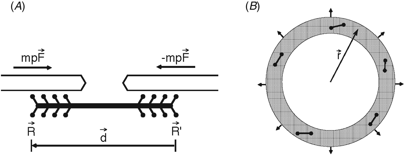
An alternative model for cellular mechanics is treating the cytoskeleton as a soft, glassy gel, and this framework was used to develop a model for the contractile ring (Carlsson, Reference Carlsson2006). Instead of a continuum description, the cortex region is assumed to have some degree of molecular structure, namely discrete myosin minifilaments that are treated as force dipoles that produce contractile stresses in the actin gel (see Fig. 3). The maximum tension that can be produced is found to depend on the length of these myosin minifilaments, the length of the actin filaments, and the circumference of the contractile ring. When experimentally measured values are put into this model, the calculated net forces are 20–30-fold too small when compared to experiment. The simplest and most reasonable way to amend this model is to include actin crosslinkers, either an explicit crosslinker such as α-actinin or some effective crosslinking due to myosin II itself. With this extension, the effective filament length is longer, and the corresponding tension in the ring is higher.
(A) Schematic of the force dipole model for a myosin minifilament. (B) Illustration of the contractile ring showing the myosin minifilaments (dumbbells) that work against surface forces that resist contraction (arrows on perimeter). Reproduced from Carlsson (Reference Carlsson2006).
Zumdieck et al. (Reference Zumdieck, Kruse, Bringmann, Hyman and Julicher2007) used a similar starting point in developing their multiscale model for cytokinesis. They include a microscopic description in which actin filaments polymerize, depolymerize, treadmill, and interact via myosin motors. This discrete model is then coarse-grained into a continuum description, where the dynamics of filaments with different orientations are captured by a polar filament concentration that changes due to diffusion, active sliding, polymerization, and depolymerization. Finally, these concentration profiles from the continuum description are interpreted in terms of a phenomenological model that considers the stresses these filament bundles produce, and how this results in constriction. Despite this multiscale approach, the overall model is fairly simple, and its predictions match experimental results very well (in this case, Caenorhabditis elegans cell division).
Building upon the active polar gel theory for the actin cortex (Kruse et al. Reference Kruse, Joanny, Jülicher, Prost and Sekimoto2005), Salbreux et al. (Reference Salbreux, Prost and Joanny2009) developed a model, where the cortical flow of actin is coupled to the orientation of the filaments. This model has many features reminiscent of liquid crystal physics, and due to the coupling between the hydrodynamic flow and filament orientation, the filaments move to the cell equator and are nematically ordered into a ring. In this case, the cortical flow and ring formation is driven by a gradient of myosin activity that is imposed on the cortical layer. This differs from the description of Zumdieck et al. above where ring formation arises from instability. Apart from formation of the contractile ring, the authors additionally show how their model does an adequate job of describing wound healing in the cortex of Xenopus eggs.
As discussed above, He and Dembo (Reference He and Dembo1997) assumed a diffusible messenger molecule as a method for triggering ring contraction, but this initiation could also arise from mechanical instability. This is precisely what Shlomovitz and Gov propose (Shlomovitz & Gov, Reference Shlomovitz and Gov2008). In contrast to previous mechanical models that considered uniform, cell-wide contraction that resulted in a contractile ring at the cell equator, they consider a distributed contractile network that can spontaneously aggregate into a contractile ring. This aggregation process is tied to the curvature of the membrane, and their general model can be applied to a wider range of cell and membrane geometries, including concave and convex deformations. The equations are complex, but the physical underpinnings are relatively simple, and actually correspond quite closely to the Monte Carlo model of Vavylonis et al. (Reference Vavylonis, Wu, Hao, O'shaughnessy and Pollard2008) that features similar condensation of contractile elements.
Finally, some recent models of cytokinesis do consider division in metazoan cells. Sedzinski et al. (Reference Sedzinski, Biro, Oswald, Tinevez, Salbreux and Paluch2011) performed both experiments and modeling of cytokinesis in HeLa cells and fibroblasts. Their minimal model for the dividing cell considered the contractile stress in the cortex and the resulting Laplace-like pressure. If the cleavage furrow is exactly in the middle of the cell, the forces are symmetric. However, they assigned a linear, bulk elasticity to the cell interior that resists deformation and thus could stabilize the cell against instabilities arising from loss of symmetry in either the volumes of the two halves and/or in the tension at the cell poles. They tested this model by introducing tension imbalances, through local delivery of cytochalasin D or laser ablation at one pole, and found that they can induce shape instabilities, and even oscillations in cell shape. Their simple model reproduced the instabilities, but not the observed oscillations. However, when they accounted for turnover of the cortex and concomitant tension relaxation at the poles, their model could quantitatively match experimental data. This model has clear applications to asymmetric cell division and more broadly indicates that dynamics and turnover of the cortex, not just its mechanics, will be important considerations in future work.
2.4 Putting it all together
At first glance, it can be a challenge to find unifying themes and conclusions from the array of models that have been developed, particularly given the differences in biological systems and the types and levels of modeling. However, there are some commonalities, as well as clear discrepancies, and they are worth highlighting.
With regard to contractile ring assembly, the ‘search, capture, pull and release’ or ‘node’ model and the ‘leading cable’ model are in essence not too different from each other. The primary distinction between them is their assumed distribution of the formin cdc12p. However, both models assume similar components in the cortical patches (actin, myosin, and formins). One advantage of the node model relative to the leading cable model is that it has been built up through careful and detailed biochemistry, combined with quantitative modeling. The truth may be somewhere in between these two models, at least for the case of fission yeast, and future experiments and models will need to tease out the details of ring assembly in other eukaryotic systems.
In the case of ring contraction, there is more diversity among the various models, but the majority of the differences come down to the model system that is being studied. For example, the Robinson and Iglesias labs have performed extensive experiments and highly quantitative modeling in the case of Dictyostelium, but many of the details of these models are specific to Dictyostelium and transferability to other systems like C. elegans or animal cells may have some challenges. It is important, however, to transcend the details of a particular scheme and recognize the larger scale physics that governs each model and description. When we step back, we see that in basically all systems considered the mechanics of cytokinesis have three primary contributors: the mechanics of the cortex, the viscoelastic properties of the cytoplasm, and constriction at the cell equator. The relative contribution of each element may differ from system to system, and the experiments using cytochalasin D discussed above are good examples of this. But all three contributions are still present and contribute, at least in some form, to the mechanics of cytokinesis. In addition to these three physical factors, the Laplace pressure is another unifying feature in many of the models and cell types. Future experiments and modeling efforts will likely find even more points of commonality, hopefully resulting in a general understanding of this process across a wide range of model systems.
3. Cell polarization and F-actin waves
In discussing cell polarization and actin waves, our focus will be on the nature of the activating and inhibitory protein interactions that lead to polarization or wave formation. We also describe agent-based models in the same framework as models based on partial differential equations, so that the physical assumptions can be directly compared. We will take a limited definition of cell polarization: a distribution of F-actin that is persistent in a way that can lead to cell migration. The asymmetry may result from (i) a temporary asymmetric stimulus, such as a growth factor or mechanical force, which is subsequently removed or (ii) a uniform stimulus that causes the symmetric state to become unstable. Since we focus on polarization that can lead to migration, we do not treat polarization in yeast, which has been treated extensively. Reviews are given in (Drake & Vavylonis, Reference Drake and Vavylonis2010; Johnson et al. Reference Johnson, Jin and Lew2011; Mogilner et al. Reference Mogilner, Allard and Wollman2012; Mullins, Reference Mullins2010; Thompson, Reference Thompson2013; Welf & Haugh, Reference Welf and Haugh2011). We also restrict ourselves to models that produce polarization that is self-generated in the sense that it develops or persists in the absence of asymmetric external stimulus; we do not treat chemotaxis.
Polarization of F-actin involves a number of upstream cellular factors, including:
(i) Membrane lipids. The conversion of PIP2 to PIP3 in the membrane, catalyzed by PI3 kinase (PI3K) stimulates localized actin polymerization (Insall & Weiner, Reference Insall and Weiner2001). The reverse PIP3–PIP2 transition is catalyzed by PTEN.
(ii) The Rho GTPase proteins, including Ras, Rac, Rho, and Cdc42. These proteins act upstream of actin polymerization and generate different types of actin structures (Raftopoulou & Hall, Reference Raftopoulou and Hall2004).
(iii) Nucleation promoting factors (NPFs), such as WASP, N-WASP, and WAVE complex. In response to upstream stimuli, they activate the Arp2/3 complex, which in turn generates new actin filaments by branching off existing ones (Pollard & Borisy, Reference Pollard and Borisy2003). This generates a branched actin network.
(iv) Myosin. Myosin II generates contractile stress in non-muscle cells as well as in muscle cells.
(v) Membrane tension. The application of force at one end of keratocyte cell fragments can persistently polarize them (Verkhovsky et al. Reference Verkhovsky, Svitkina and Borisy1999). Furthermore, membrane tension is a key factor in neutrophil polarization (Houk et al. Reference Houk, Jilkine, Mejean, Boltyanskiy, Dufresne, Angenent, Altschuler, Wu and Weiner2012).
Typical front constituents include F-actin, PIP3, Ras, Rac, and NPFs; rear constituents include PTEN, myosin, and Rho.
Some of the interactions between these constituents have been identified in the literature, and are summarized by Dawes & Edelstein-Keshet (Reference Dawes and Edelstein-Keshet2007). Important examples are the following: Ras activates PI3 kinase (Yang et al. Reference Yang, Shin, Lee, Kim, Park, Cho, Meyer and Heo2012), which causes synthesis of PIP3, PIP3 activates Rac, and Rac in turns activates NPFs. There is a network of positive and negative interactions between the Rho GTPases Rac, Rho, and Cdc42, and these may feed back onto PIP3 production. There is also a positive feedback circuit involving F-actin, PIP3 production, and Ras (Firtel et al. Reference Firtel, Sasaki, Janetopoulos, Lee, Charest, Takeda, Sundheimer, Meili and Devreotes2007). Myosin activity can lead to several types of interactions with the actin network, including active transport and network disassembly (Wilson et al. Reference Wilson, Tsuchida, Allen, Barnhart, Applegate, Yam, Ji, Keren, Danuser and Theriot2010). There is significant crosstalk between the front and rear constituents, which may be mediated by the cortical cytoskeleton or by the membrane itself. Inhibition of myosin II at the rear of chemotaxing cells leads to excessive Ras activation in the rest of the cell (Lee et al. Reference Lee, Shen, Robinson, Briggs and Firtel2010), and this effect could be mediated by the cytoskeleton. Cells depleted of dynacortin, which mechanically stabilizes the actin cytoskeleton, are less polarized than wild-type cells (Kabacoff et al. Reference Kabacoff, Xiong, Musib, Reichl, Kim, Iglesias and Robinson2007). On the other hand, a combination of blebbistatin treatment to reduce cortical contractility, and variation of osmotic pressure using hypertonic/hypotonic buffers, suggested that the plasma membrane itself, rather than the cytoskeleton, transmits the tension (Houk et al. Reference Houk, Jilkine, Mejean, Boltyanskiy, Dufresne, Angenent, Altschuler, Wu and Weiner2012). Increasing membrane tension inhibits actin polymerization, while conversely actin polymerization increases membrane tension (Houk et al. Reference Houk, Jilkine, Mejean, Boltyanskiy, Dufresne, Angenent, Altschuler, Wu and Weiner2012; Lieber et al. Reference Lieber, Yehudai-Resheff, Barnhart, Theriot and Keren2013).
F-actin waves are in some ways a dynamic variant of cell polarization. They consist of propagating fronts of actin polymerization, moving either radially or rotating around a cell. They are seen most clearly in total-internal reflection (TIRF) studies that image polymerized actin within a few hundred nanometers of the substrate. They have been seen in Dictyostelium (Bretschneider et al. Reference Bretschneider, Anderson, Ecke, Muller-Taubenberger, Schroth-Diez, Ishikawa-Ankerhold and Gerisch2009; Gerisch, Reference Gerisch2010; Gerisch et al. Reference Gerisch, Bretschneider, Muller-Taubenberger, Simmeth, Ecke, Diez and Anderson2004), neutrophils (Millius et al. Reference Millius, Dandekar, Houk and Weiner2009; Weiner et al. Reference Weiner, Marganski, Wu, Altschuler and Kirschner2007), and melanoma cells (Giannone et al. Reference Giannone, Dubin-Thaler, Dobereiner, Kieffer, Bresnick and Sheetz2004).
The waves have numerous constituents, but for simplicity we will call them F-actin waves. Many of their constituents are shared with cell polarization, including Arp2/3 complex, NPFs, membrane lipids, and Rho GTPases. The NPFs form a narrow region at the front of the wave, with F-actin and Arp2/3 complex more broadly distributed. The waves are associated with boundaries between PIP3-rich and PIP3-poor regions in the membrane. Activities of the Rho GTPases Ras (Gerisch et al. Reference Gerisch, Ecke, Wischnewski and Schroth-Diez2011) and Rac (Weiner et al. Reference Weiner, Marganski, Wu, Altschuler and Kirschner2007) are also enhanced in the waves. The front and rear constituents of waves have a strong overlap with the front and rear constituents of a polarized cell (Gerisch et al. Reference Gerisch, Schroth-Diez, Muller-Taubenberger and Ecke2012). However, actin waves in Dictyostelium do not require contractile myosin II activity (Bretschneider et al. Reference Bretschneider, Anderson, Ecke, Muller-Taubenberger, Schroth-Diez, Ishikawa-Ankerhold and Gerisch2009), although they do require the 14-3-3 protein, which modulates myosin II assembly into minifilaments (Zhou et al. Reference Zhou, Kee, Poirier, Jelinek, Osborne, Divi, Surcel, Will, Eggert, Muller-Taubenberger, Iglesias, Cotter and Robinson2010).
Key features of the waves are that they:
(i) appear at reduced actin concentrations,
(ii) annihilate upon collision,
(iii) cause protrusion of the cell membrane,
(iv) disappear under treatment of PI3 kinase inhibitors, and
(v) move by a ‘treadmilling’ motion in which the wave propagates by the addition of new material at the front, rather than by the motion of existing material.
The interaction of traveling F-actin waves with the cell membrane can lead to wavelike behaviors of the edge of the cell. There have been several theories of these cell edge waves, reviewed by Allard & Mogilner (Reference Allard and Mogilner2012) and Ryan et al. (Reference Ryan, Watanabe and Vavylonis2012). However, to keep the scope manageable, we will limit this review to waves moving in the interior of the cell.
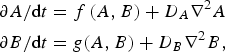
Polarized or wavelike distributions of F-actin could result from several types of generic mechanisms (Gierer & Meinhardt, Reference Gierer and Meinhardt1972). One mechanism is based on positive feedback of a constituent A (or combination of constituents), called an ‘activator’, and negative feedback of an ‘inhibitor’ B. This is compactly described within the following ‘reaction–diffusion’ framework:
 $$\eqalign{\partial A/{\rm d}t &= f\,{\rm (}A,B{\rm )} + D_A \nabla ^{\rm 2} A \cr \partial B/{\rm d}t &= g{\rm (}A,B{\rm )} + D_B \nabla ^{\rm 2} B{\rm,}}$$
where the functions f and g describe chemical reactions and the remaining terms describe diffusion. By positive feedback we mean that over some range of concentrations, ∂f/∂A > 0, so that an increase in A will feed back on itself. If unchecked, this process would lead to exponential growth of A; therefore, the positive feedback must cut off at large values of A. The inhibitor generally satisfies ∂g/∂A > 0, so that A causes growth of B, but ∂f/∂B < 0, so that B inhibits growth of A. Spreading mechanisms for A and B, described by the D A and D B terms, are also required to achieve spatial segregation. However, these terms do not necessarily have to result from diffusion (Carlsson, Reference Carlsson2010; Doubrovinski & Kruse, Reference Doubrovinski and Kruse2008).
Two general scenarios are possible depending on the relative spreading rates of A and B:
(i) If B spreads much more rapidly than A, then an initial buildup of A, resulting from a localized random fluctuation, causes a more extended distribution of B, which prevents further spreading of A. This gives static polarization.
(ii) If B spreads less rapidly than A, or at a comparable rate, the following scenario can occur: A random fluctuation creates a localized pulse of A that grows and spreads. Then B builds up, and is highest at the center of the pulse because it has had the most time to build up there. Because of the inhibitory action of B, the buildup of B causes the middle of the A pulse to drop out, and the two fronts on either side travel in opposite directions into regions where the lower B concentration favors growth of A. This gives traveling waves. The driving force for wave propagation is thus the spatial gradient of B.
Within these general mechanisms, two broad classes of behaviors are possible:
(i) Instability. Here symmetric and polarized/wave-forming regimes appear as parameters vary, and for a given set of parameters either a symmetric or polarized state is stable, but not both. The transition to polarization or wave formation results from an instability in the steady-state solutions analogous to that of a roller coaster sitting at the very top of its track, from where it can drop in either direction. This means that even very small perturbations will cause polarization or wave formation.
(ii) Threshold behavior. Here the symmetric state is stable until it experiences a sufficiently strong perturbation. If polarization occurs, the polarized state persists; but if a wave forms it may be persistent or transient. For given parameter values, two or more steady-state solutions may exist. Threshold polarization behavior occurs naturally in models which are ‘bistable’. This means that one or both of Eqs. (1), when treated without spatial variation (so that they become ordinary differential equations), have two stable solutions. Threshold behavior in wave-forming systems occurs in extensions of classical ‘FitzHugh–Nagumo’ models (FitzHugh, Reference Fitzhugh1961; Vasiev, Reference Vasiev2004). In these models, small concentrations of A are stable, so that dA/dt < 0, but at larger values of A positive feedback ‘kicks in’ and dA/dt becomes positive. If A is pushed beyond this threshold by a random fluctuation, the system undergoes a long excursion corresponding to a wave.
A variant of the general mechanism of Eqs. (1) assumes conservation of one of the constituents. For example, A can have active and inactive forms A* and A, with the total A* + A in the cell being independent of time. Often A* is taken to be membrane-localized and A is cytosolic, but they can both be membrane-localized. The inhibitor B in the latter case is depletion of inactive A. If the A→A* transition feeds positively back on itself, polarization can result from local buildup of A* combined with depletion of A, which is usually taken to diffuse faster than A*. If the model is bistable, the cell has two regions, each having a relatively constant value of A* equal to one of the two steady-state solutions. Such polarization models can produce waves if a second, slowly diffusing, inhibitor is included.
4. Cell polarization models
The activator–inhibitor mechanism described above has been the basis of most of the polarization models studied to date. Most have assumed that the activator is at the front of the cell, but some have taken it at the back, and only a few have treated activators at both front and back. Polarization can also result from other related mechanisms. For example, one could envisage a mechanism based entirely on mutual inhibition, where buildup of A inhibits B and buildup of B inhibits A. Such a mechanism requires continual influx of A and B, but not positive feedback. Furthermore, if A is produced spontaneously throughout the cell, and there is a mechanism for concentrating it, there is not a need for a separate inhibitor.
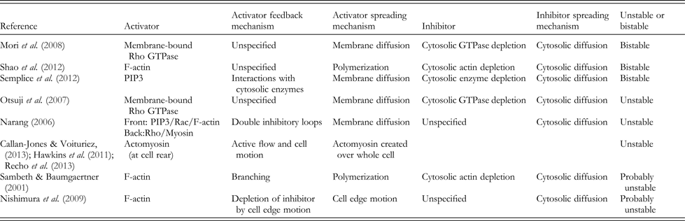
We divide the models into those having thresholds for polarization and those having instabilities. In some cases, this distinction was not made explicit, and here we have used our best judgment, with our apologies to the authors if our judgment erred. The key features of cell polarization models are summarized in Table 1.
Key features of static polarization models. In all cases based on reaction–diffusion equations, D i (inhibitor diffusion coefficient)>>D a (activator diffusion coefficient)
4.1 Threshold models
A mechanism based on shuttling between active A* and inactive A was studied by (Mori et al. Reference Mori, Jilkine and Edelstein-Keshet2008), where A* corresponds to active, membrane-bound Rho GTPase. The model abstracted key features from a previous more complete biochemical treatment (Dawes & Edelstein-Keshet, Reference Dawes and Edelstein-Keshet2007). The GTPase could shuttle into the cytosol, where it became inactive (A), and back onto the membrane. Positive feedback was included via a cubic nonlinearity in the growth law. The geometry treated was a one-dimensional (1D) strip corresponding to a rectangular cell that is uniform in the direction transverse to the motion. The system was bistable with homogeneous steady-state values A*− and A*+. Beginning in the A*− state, imposition of a localized increase of A* resulted in a stable polarized steady state, with A* elevated at one side of the cell. As seen in Fig. 4, there are well-defined plateaus having different values of A* = A*− (zero in this case) and A* = A*+. This model captured key features of cell polarization, including the ability to amplify a stimulus to attain a polarized state, the ability to retain polarization after the stimulus is removed, the ability to reverse polarization in response to a sufficiently strong second signal, and the ability to polarize in response to a spatially random signal.
Wave-pinning model of cell polarization. A pulse of membrane-bound activator stops moving when the cytosolic concentration reaches a critical level. Reproduced from Mori et al. (Reference Mori, Jilkine and Edelstein-Keshet2008).
The work of Shao et al. (Reference Shao, Levine and Rappel2012) extended this general idea to two dimensions and included effects of actomyosin contraction. Via use of a phase-field method, where a function of position defines inside versus outside of the cell, they treated a deformable boundary. Using this model, they considered an initially circular cell. After perturbation by a pulse of F-actin at the front, the asymmetry in the actin distribution persisted, and the cell deformed, becoming longer in the direction transverse to its motion (see Fig. 5). Myosin moved to the rear of the cell. A phase diagram of cell shapes as a function of cell-substrate adhesion strength and myosin activity was obtained, in which cell asymmetry was most favored at a point where myosin activity and cell-substrate adhesion are intermediate.
A cell evolving from a circular starting state to a polarized migrating state in an activator-inhibitor model including myosin. (A) Three successive snapshots of cell developing asymmetry. (B) Steady-state polymerized-actin distribution. (C) Steady-state myosin distribution. Reproduced from Shao et al. (Reference Shao, Levine and Rappel2012).
Another bistable mechanism was treated by (Semplice et al. Reference Semplice, Veglio, Naldi, Serini and Gamba2012), assuming two activators, A = PIP3 and A′ = PIP2, both in the cell membrane. The total A + A′ was conserved, and transitions between A and A′ were caused by PI3K and PTEN. Positive feedback interactions were assumed from both PIP3 to PI3K, and from PIP2 to PTEN, giving two activators. The boundary of the PIP3 region was determined by the relative concentrations of active PI3K and PTEN, which were coupled to A and A′. Assuming rapid equilibration of these couplings, the system was described by a single variable ϕ = A−A′. The time evolution of ϕ, in turn could be described by an ‘energy function’ V(ϕ) (not a physical energy). This gives a heuristic way of predicting the direction of change. The function V(ϕ) has two minima corresponding to stable steady states. The boundary between these two states in the cell will be stationary when the depths of the two minima are equal, so that there is no net ‘energy’ gain from moving the front. This model predicted polarization in response to uniform stimulation, and also suggested that a ‘coarsening’ process should be a general feature of the transition from a quiescent state to a polarized equilibrium. In this process, initial nuclei of the new, high-ϕ phase, are nucleated and grow. The resulting depletion of cytosolic components limits the formation of new nuclei by increasing the required critical nucleus size. The existing nuclei, however, continue to grow and merge, eventually forming a single large cap at one end of the cell.
A simplified bistable model, based on mechanical variables (Kozlov & Mogilner, Reference Kozlov and Mogilner2007), treated the bistable behavior of cell fragments (Verkhovsky et al. Reference Verkhovsky, Svitkina and Borisy1999) mentioned above. The cell was assumed to either be circular, or to have a simple parameterized shape with a circular leading edge and a scallop taken out of the rear of the cell. Actin polymerization forces were taken to act at the leading edge, while actomyosin network contraction occurred on an interior ring concentric with the leading edge. Finally, a contractile bundle was assumed to be present along the rim of the scallop at the rear of the cell. The mechanical energy of the cell contained contributions from (i) the forward motion of the leading edge of the cell in response to the force of actin polymerization, (ii) the contracting actomyosin network farther inside the cell, and (iii) the contractile bundle at the rear. The energy at mechanical equilibrium was written in terms of the angle ϕ subtended by the scallop at the rear of the cell, so that ϕ = 0 corresponds to a circular cell fragment. For small ϕ, the energy initially increased because of the energy of extending the bundle at the cell rear, so that the circular shape was locally stable. However, at larger ϕ, the energy dropped, because the asymmetry of the front of the cell allowed it to move and thus lower the actin polymerization energy. Finally, at still larger values of ϕ, the energy rose. Thus there were two stable energy minima, which could correspond to the moving and stationary cell fragments seen in the experiments. Because this model is based on a small number of variables, the mechanisms cannot be directly compared to those discussed above. Nevertheless, there is a positive feedback mechanism that drives ϕ to larger values once it has reached a certain threshold. This mechanism results from the combination of forces from actin polymerization and actomyosin network contraction, with geometric nonlinearities inherent in the cell model.
4.2 Instability models
The model of (Otsuji et al. Reference Otsuji, Ishihara, Co, Kaibuchi, Mochizuki and Kuroda2007) had a conserved front protein with active and inactive states A and A*. This model was solved in a 1D domain, and reproduced the results of a more complex model including a network of Rho GTPases. The inhibitor again corresponds to depletion of cytosolic A. In the absence of stimulation, there is a single stable steady state, in which A* and A are uniformly distributed across the cell. Under stimulation, modeled by increasing the activation rate of A, this stable steady state becomes unstable and A* grows rapidly to form a distribution that is shaped more like a peak than a plateau.
A model based on two activators A and A′ was proposed by (Narang, Reference Narang2006), where the single variable A describes PIP3, Rac, and F-actin, whereas A′ describes Rho and myosin. A and A′ were assumed to mutually inhibit each other. An additional inhibitor grows in response to A and A′, and acts back negatively on them. Stimulation is modeled as an increase of the positive feedback term for A. A stable uniform steady state was found up to a certain critical value of uniform stimulation. Past this value, the system becomes unstable and the front and back proteins segregate. This model reproduces two phenomena that are not captured by two-variable models: (i) Expansion of the back proteins into a larger proportion of the cell when the front pathway is suppressed. In models where the back proteins are the inhibitor, the back proteins would decrease when the front pathway is suppressed. (ii) Chemorepulsion. A transition from chemoattraction to chemorepulsion could be caused by appropriately balancing the front and back pathways.
Models have also been proposed based on spontaneous assembly of myosin at the rear of the cell, where A is the concentration of myosin or actomyosin (Callan-Jones & Voituriez, Reference Callan-Jones and Voituriez2013; Hawkins et al. Reference Hawkins, Poincloux, Benichou, Piel, Chavrier and Voituriez2011; Recho et al. Reference Recho, Putelat and Truskinovsky2013). These models build on earlier work showing that active myosin stresses can induce patterns in uniform systems (Bois et al. Reference Bois, Julicher and Grill2011; Mayer et al. Reference Mayer, Depken, Bois, Julicher and Grill2010; Salbreux et al. Reference Salbreux, Joanny, Prost and Pullarkat2007). These models do not have the mathematical form of the reaction–diffusion equations above, but rather involve a globally produced activator, taken to be myosin, which is accumulated at the rear of the cell. Positive feedback causing myosin accumulation results from two physical effects: (i) Active contractile currents, which compress the actomyosin gel and thus increase the concentration. (ii) Cell motion, where forward motion of the cell naturally leaves the actomyosin gel at the rear of the cell. Accumulation is eventually halted by either diffusion, actomyosin disassembly, or both. These models should be especially relevant to migration in three dimensions. They were able to reproduce the actomyosin concentration and active flow velocity as a function of angle going around the cell. They also found that the transition to a polarized state is driven by the Peclet number, which quantifies the importance of advection (driven by active transport) relative to diffusion.
A stochastic model that gives a polarization instability was treated by (Sambeth & Baumgaertner, Reference Sambeth and Baumgaertner2001), where A* corresponded to F-actin and A to free actin. The system treated consisted of a square region in two dimensions, with front and rear boundaries elastically coupled. Actin polymerization based on branching from Arp2/3 complex was treated using an agent-based method that stored explicit filament coordinates over time. The formation of new branches was allowed only near the membrane, and the actin filaments that were in networks were assumed to be ‘glued’ to the substrate, allowing them to push the cell forward. The positive feedback in this model results from branching of actin filaments: the rate of creation of new actin is (roughly) proportional to amount of actin present. Because of conservation of total actin, actin polymerization proceeded until the free-monomer concentration became so small that depolymerization balanced polymerization. This model produced spontaneous polarization, but with the direction of polarization slowly fluctuating back and forth. The polarization did not have a well-defined value, but rather meandered during the course of the simulations. Thus there do not appear to be sharp transitions in this model, but rather gradual changes with increasing polymerized-actin content, in which the magnitude and lifetime of the polarization grow.
Another stochastic model based on the interaction between cell boundary motion and a cortical inhibitor was treated by Nishimura et al. (Reference Nishimura, Ueda and Sasai2009). F-actin was assumed not to diffuse, while the inhibitor spread randomly from a given site on a hexagonal lattice to another site at a rate proportional to its diffusion coefficient. Actin polymerization occurred only if the inhibitor concentration in a given cell was below a threshold value. The polarization mechanism relied on F-actin pushing the membrane forward, thereby locally depleting the inhibitor. At the same time, retraction of the rear of the cell increased the inhibitor concentration there. This model does not have an activator in the sense of the preceding models. Rather, the positive feedback comes indirectly from the combination of two negative feedback effects: F-actin reduces the inhibitor concentration locally by stretching the cell, while the inhibitor reduces actin polymerization by assumption. By varying parameters in the model, a range of dynamic polarization behaviors were observed (Fig. 6), with some corresponding to the steady-state motion of keratocytes, and others giving more random amoeboid-like motion like that of Dictoystelium.
Migration of a cell in polarization model based on positive feedback of F-actin onto itself, via depletion of an inhibitor. Color indicates inhibitor concentration. Reproduced from Nishimura et al. (Reference Nishimura, Ueda and Sasai2009).
5. F-actin wave models
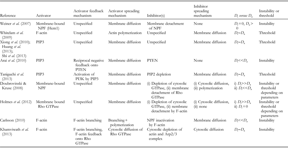
Because actin-wave models have used a very wide variety of assumptions and methodologies, we feel that the relationships between models are seen most clearly by dividing them according the general mechanism used to obtain waves, as well as their mathematical methodology. Key features of F-actin wave models are summarized in Table 2.
Key features of F-actin wave models. D i and D a are inhibitor and activator diffusion coefficients
5.1 Extensions of classical oscillator systems
The model of (Weiner et al. Reference Weiner, Marganski, Wu, Altschuler and Kirschner2007) took the activator A is the active, membrane-bound form of the NPF Hem-1, and the inhibitor B as F-actin. The model was implemented on a discrete mesh, assuming that buildup of A on a given node is aided by A already present on that node and on neighboring nodes. In response to Hem-1, F-actin builds up, and inhibits Hem-1 by pulling it off the membrane and thus inactivating it, consistent with their experimental data. It was found that (i) circular waves move outward with a spacing determined mainly by the lifetime of F-actin, (ii) colliding waves annihilate, and (iii) depolymerizing actin freezes Hem-1 waves and increases their intensity, consistent with their experimental observations.
In contrast, Whitelam et al. (Reference Whitelam, Bretschneider and Burroughs2009) viewed F-actin as A and assumed B to be a depolymerization agent. They treated two effects not present in the FitzHugh–Nagumo models. The first is directed motion parallel to actin filaments; filament alignment was assumed to appear spontaneously. The second is random fluctuations in A. This model produced a sequence of phases, beginning with stationary spots, changing to moving spots, and finally transforming to traveling waves. This sequence of phases is consistent with the sequence (Gerisch et al. Reference Gerisch, Bretschneider, Muller-Taubenberger, Simmeth, Ecke, Diez and Anderson2004) that was experimentally observed in Dictyostelium recovering from actin depolymerization.
The treatment of Xiong et al. (Reference Xiong, Huang, Iglesias and Devreotes2010) took A to be PIP3, while B was unspecified. The nonlinearity in the evolution equation for A was chosen to obtain ‘excitable’ behavior, where a small but finite initial perturbation induces a large burst of activity. The parameters were chosen to roughly match the dynamics of PIP3 patches in Dictyostelium. When a random time series of perturbations was applied to the system, waves nucleated both in the interior and around the edge of the cell. The waves nucleated as patches and subsequently spread to coherent structures roughly the size of the cell. Uniform stimulation resulted in an initial strong response, which later converted to transient patches. Later extensions of this work have treated the coupling of the excitable signaling network to the cytoskeleton in different ways, reproducing key cellular behaviors such as random protrusion (Huang et al. Reference Huang, Tang, Shi, Iglesias and Devreotes2013; Shi et al. Reference Shi, Huang, Devreotes and Iglesias2013).
In the model of Arai et al. (Reference Arai, Shibata, Matsuoka, Sato, Yanagida and Ueda2010), the activator was again taken as membrane bound PIP3, and the inhibitor as PTEN, an enzyme that reverses PIP3 synthesis. Reciprocal negative feedback between PIP3 and PTEN led to spatial separation of these constituents. This model led to a range of behaviors along the cell edge, including both traveling waves and standing waves. In a related model by Taniguchi et al. (Reference Taniguchi, Ishihara, Oonuki, Honda-Kitahara, Kaneko and Sawai2013), the activator A is also membrane-bound PIP3, whereas the inhibitor B is absence of PIP2. PTEN, and the enzyme PI3K that drives PIP3 synthesis, were treated as rapidly equilibrating, justifying a model based only on A and B. The key positive feedback was from a loop involving PIP3 and PI3K. The model was explored in a two-dimensional (2D) spatial domain (see Fig. 7), systematically varying parameters. Weak positive feedback led to individual waves that travel across the cell and extinguish at the other boundary. Moderate feedback strength led to either spiral or reflecting waves. At still higher levels of positive feedback, excitability was lost and no waves could propagate. Colliding waves were found to annihilate, again consistent with the experimental data. This work also treated the effect of a deformable boundary, using a phase-field method (Shao et al. Reference Shao, Levine and Rappel2012). The boundary deformability had a strong effect on wave reflection from the boundary, which occurred for either high deformability or low deformability, but not in between.
Different wave and patch structures formed in an actin wave model based on interconversion between PIP3 and PIP2. Red is PIP3 and green is PIP2. Columns A-D give results for increasing positive feedback strength. Reproduced from Taniguchi et al. (Reference Taniguchi, Ishihara, Oonuki, Honda-Kitahara, Kaneko and Sawai2013).
5.2 Extensions of static polarization models by adding a second inhibitor
Two models (Doubrovinski & Kruse, Reference Doubrovinski and Kruse2008; Holmes et al. Reference Holmes, Carlsson and Edelstein-Keshet2012) have added a second inhibitor to polarization models such as that of Mori et al. (Reference Mori, Jilkine and Edelstein-Keshet2008). They assume the activator A* to be a nucleation-promoting factor (Doubrovinski & Kruse, Reference Doubrovinski and Kruse2008) or a Rho GTPase (Holmes et al. Reference Holmes, Carlsson and Edelstein-Keshet2012) and, like Weiner et al. (Reference Weiner, Marganski, Wu, Altschuler and Kirschner2007), take the inhibitor to be F-actin. In these models, a wave can be initiated by a pulse of A* at one end of the cell. This pulse grows rapidly until cytosolic A is depleted. Then the negative feedback from F-actin builds up slowly, and the A* peak moves across the cell to regions having lower inhibitor concentration. In Doubrovinski & Kruse (Reference Doubrovinski and Kruse2008) a phase diagram of possible behaviors in two dimensions was evaluated in terms of the strength of the positive feedback in the A→A* reaction, and the F-actin spreading rate. F-actin was taken to spread via polymerization rather than diffusing via Brownian motion. It was shown that polymerization, in certain limits, is mathematically equivalent to diffusion. With increasing positive feedback strength, they found a transition from a uniform homogeneous state to states structured either in space or in space and time. The stationary states were those with smaller effective F-actin diffusion coefficients. This model was extended to treat a flexible boundary (Doubrovinski & Kruse, Reference Doubrovinski and Kruse2011), by treating the boundary as a string in two dimensions whose velocity was determined by the force from the actin filaments and the membrane mechanical properties. It was found that F-actin waves can generate directional cell motion, and also that the presence of the boundary can cause the F-actin waves to propagate along the membrane.
The calculations of Holmes et al. (Reference Holmes, Carlsson and Edelstein-Keshet2012) explored possible behaviors in terms of the strength of the negative feedback from F-actin and the baseline term in the A→A* transition, in a 1D model. With increasing negative feedback a series of spatiotemporal patterns was obtained including both static polarization and reflecting waves (see Fig. 8). The first transition was from static polarization to mildly oscillating polarization in which the direction of polarization remained the same but the magnitude varied periodically over time. The second transition was to traveling waves, which traversed the cell, reflected from the boundary, and traveled back in the opposite direction. Using different parameter variations led to other phases, such as ‘wave trains’ in which a wave would initiate at one boundary, travel to the other boundary and be extinguished. A new wave would then initiate at the first boundary.
Transition from static polarization to reflecting behavior seen in model with positive NPF self-feedback, and F-actin as an NPF inhibitor. Top frame: low inhibition strength. Lower frame: high inhibition strength. Reproduced from Holmes et al. (Reference Holmes, Carlsson and Edelstein-Keshet2012).
5.3 Single-variable models
The model of Westendorf et al. (Reference Westendorf, Negrete, Bae, Sandmann, Bodenschatz and Beta2013) treated oscillations of a single dynamical variable, the cortical polymerized actin content in Dictyostelium. They obtained oscillations within this model using a delay term. The polymerization rate contained a positive feedback term, whose physical origin was not specified, but which might be connected with the F-actin-PI3K positive feedback circuit (Firtel et al. Reference Firtel, Sasaki, Janetopoulos, Lee, Charest, Takeda, Sundheimer, Meili and Devreotes2007) mentioned above, or positive feedback from branching (Carlsson, Reference Carlsson2010; Sambeth & Baumgaertner, Reference Sambeth and Baumgaertner2001). Actin depolymerization was described by a delayed quadratic decay term, based on the amount of F-actin at an earlier time. The delay was justified in terms of possible delays in the binding of depolymerizing protein. With increases in either the delay time or the positive feedback coefficient, the system undergoes a transition from a stable steady state to an oscillating state. For parameter values slightly below the transition point, a pulse stimulus caused an oscillatory response with a decaying envelope. This model reproduces the experimental data (Westendorf et al. Reference Westendorf, Negrete, Bae, Sandmann, Bodenschatz and Beta2013) for a population of Dictyostelium cells, some of which oscillated spontaneously, while others displayed decaying oscillatory responses to cAMP stimulation.
5.4 Detailed biochemical and/or structural models
Rather than assume simplified two- or three-variable systems, these models attempt to capture as much of the known biochemistry as possible, and ‘let the chips fall where they may’. The key activators and inhibitors then emerge from the simulation results.
The work of Carlsson (Reference Carlsson2010) extended the earlier branching-based cell polarization model (Sambeth & Baumgaertner, Reference Sambeth and Baumgaertner2001) to treat actin waves. In addition to adding several biochemical processes to the model, such as barbed-end capping of actin filaments, a density of NPFs varying over the 2D area of the cell was introduced. The rate of branching was taken to increase quadratically with the local NPF concentration. It was also assumed, as in several other models, which F-actin detaches NPFs from the membrane, and thus inactivates them. Simulations of this model showed a range of phases including static patches, moving patches, and traveling waves, with increasing actin concentration. This is a variation similar to that seen by Whitelam et al. (Reference Whitelam, Bretschneider and Burroughs2009), but as a function of actin concentration rather than time. Since the phases were experimentally observed under conditions of recovery from depletion of polymerizable actin, their transitions may well result from growing actin concentration. In this model, the activator is F-actin and the inhibitor is depletion of NPF. As in (Sambeth & Baumgaertner, Reference Sambeth and Baumgaertner2001) positive feedback comes from branching, while branching and polymerization together give diffusion-like spreading. Finally, negative feedback comes the detachment of NPFs from the membrane by F-actin.
In a biochemical model treating more upstream signaling events, Khamviwath et al. (Reference Khamviwath, Hu and Othmer2013) treated continuous densities of actin filament barbed and pointed ends, G-actin, Arp2/3 complex, the NPF WASp, the Rho GTPase Rac, and the depolymerizing factor coronin, on a flat membrane and in the cytosol. The actin filament nucleation rate from branching was taken proportional to the density of barbed ends. Both active and inactive forms of WASp and Rac were treated. Different variables were treated as being cytosolic or membrane-bound, as deemed appropriate. Diffusion was treated in three dimensions for cytosolic entities, but assuming symmetry along one axis of the cell allowed the treatment of diffusion in a 2D geometry defined by the direction of motion of the wave (x) and distance from the membrane (z). The wave was initiated by a transient, spatially localized increase in the nucleation rate of actin filaments. The resulting time course of actin polymerization began with a single pulse, whose intensity grew over time while the pulse spread in both the x- and z-directions (see Fig. 9). Subsequently, the middle hollowed out, and the pulse split into two symmetric pulses moving in opposite directions. The decay in the middle was caused by a combination of depolymerization induced by coronin, and a reduction of polymerization and filament nucleation from depletion of G-actin and Arp2/3 complex. The spatial profiles of the proteins are consistent with those observed by (Bretschneider et al. Reference Bretschneider, Anderson, Ecke, Muller-Taubenberger, Schroth-Diez, Ishikawa-Ankerhold and Gerisch2009). In particular, the propagating wave has the form of an initial high peak, followed by a region of fairly constant F-actin density. This structure is due to depletion of G-actin. On the other hand, the concentration of Rac (treated as a proxy for PIP3) did not display peaks, consistent with the PIP3 data of Bretschneider et al. (Reference Bretschneider, Anderson, Ecke, Muller-Taubenberger, Schroth-Diez, Ishikawa-Ankerhold and Gerisch2009). Another feature of the simulation results is that ‘by-hand’ inclusion of PTEN activity results in wave retraction, consistent with experimental observations that actin waves often propagate to the cell edge and then retract. In this model, the key positive feedback elements result from nucleation of actin filaments by branching, and interactions of F-actin with Rac. The key inhibitors are coronin, and depletion of G-actin and Arp2/3 complex.
Development of an actin wave in a model with an F-actin/Rac positive feedback loop. An initial pulse grows and spreads, with the dip in the middle resulting from depolymerization agents and cytosolic actin depletion. The colors denote polymerized-actin concentration. Reproduced from Khamviwath et al. (Reference Khamviwath, Hu and Othmer2013).
The work of Zeng et al. (Reference Zeng, Lai, Koh, Leduc and Chiam2011) treated circular dorsal ruffles (CDRs), which are closely analogous to F-actin waves propagating on the bottom of the cell. The CDRs are outward-moving rings of actin traveling along the top of a cell upon growth factor simulation, where the free membrane forms traveling ruffles in response to outward-moving actin polymerization. Zeng et al. studied a model containing most of the known components of the platelet-derived growth factor (PDGF) pathway, including the PDGF receptor (PDGFR), PI3K, Rac and Rho activators and exchange factors, and several additional proteins. The mathematical model did not contain positive feedback that would generate a wave spontaneously. Rather, the effects of a large localized pulse of PDGF were evaluated. It was found that ring of actin was generated, which persisted for about 30 min, and then decayed. The key negative feedback effect causing the wave was the buildup of factors inactivating Rac. A simpler version of this model was also implemented, based on just Rac and its exchange factor. In this model it was found that a small initial increase in Rac, induced by PDGF stimulation, would not cause any significant excursion from the stable steady state, whereas a larger initial increase would cause a pulse of Rac much as seen in the experiments.
6. Outlook
A major frontier in the study of cytokinesis on the one hand, and cell polarization/F-actin waves on the other hand, is to understand the effect of mechanical stresses on the underlying biochemistry (Goehring & Grill, Reference Goehring and Grill2013; Mogilner & Zhu, Reference Mogilner and Zhu2012). For cytokinesis, it has been shown (Kee et al. Reference Kee, Ren, Dorfman, Iijima, Firtel, Iglesias and Robinson2012) that accumulation of myosin II is controlled by a multiprotein mechanosensory network. The effect of mechanics on chemistry is shown by experiments on fragments (Verkhovsky et al. Reference Verkhovsky, Svitkina and Borisy1999) showing that application of a force could induce persistent polarization of fragments of keratocyte cells. More recently, it has been shown that tension is a key factor in the polarization of neutrophils (Houk et al. Reference Houk, Jilkine, Mejean, Boltyanskiy, Dufresne, Angenent, Altschuler, Wu and Weiner2012). The effects of mechanics on chemistry have only been included in a few of the calculations discussed above, although some of the basic mechanisms are becoming clarified (Luo et al. Reference Luo, Mohan, Iglesias and Robinson2013). In this direction, Ofera et al. (Reference Ofera, Mogilner and Keren2011) treated the interplay between membrane tension, filament force generation at the front of a cell, and filament breaking at the rear. They calculated a self-consistent polarized profile of polymerized actin, and predicted a correlation between front-to-rear distance of the cell and curvature of the leading edge, consistent with experiment.
The calculations described in Sections 4 and 5 suggest that static polarization, wave formation, and other phenomena such as random protrusion of the periphery, have enough commonality that they can be understood within a single theoretical framework. Consider, for example, the upstream PIP3/PIP2/PI3K/PTEN module, which is included in several of the models. It has been treated as a bistable system, as one that is in the uniform oscillation (instability) regime, and as an excitable system. These differing assumptions correspond to different cell phenotypes, including static polarization, regular wave behaviors, and random protrusion in the form of pseudopods. Such phenotypes could likely be obtained by tuning the parameters in a single comprehensive model. The possibility of a comprehensive model is also suggested by the calculations described above for the actin module (Doubrovinski & Kruse, Reference Doubrovinski and Kruse2008; Holmes et al. Reference Holmes, Carlsson and Edelstein-Keshet2012). They suggested two avenues by which static polarization can convert to wave behavior: slowing inhibitor diffusion and increasing the strength of the negative feedback. There are also more complex dynamic phases that could be treated, including oscillatory polarization, actin patches, and other dynamic phases where F-actin is highly dynamic but does not show clearly definable waves or patches. In addition, the types of behaviors seen here have subclasses. For example, F-actin waves could either reflect from the cell edge, or appear in trains starting at one point in the cell. A model that can reliably predict such transitions in F-actin dynamic behavior in terms of variations in the activity/expression of key proteins and pharmacological treatments would go a long way toward a comprehensive theory.
Since such models would make concrete predictions for a broad range of phenotypes, they would enhance our ability to identify the key positive and negative feedback elements that drive polarization or actin waves in particular systems. The testing and validation of such models will be greatly enhanced by more extensive fluorescence studies imaging two constituents at a time. As demonstrated in the more limited network of proteins driving endocytosis in yeast (Kaksonen et al. Reference Kaksonen, Toret and Drubin2005), a systematic combination of a large number of such double-labeling studies can give a detailed picture of protein dynamics that provides strong constraints on mathematical models. Such concomitant advances on both the modeling and experimental fronts have mutual benefit for each side, and together they suggest a bright future for understanding cellular dynamics and organization.
7. Acknowledgements
This work was supported by the National Institutes of Health under Grant Number R01 GM107667 to A.E.C.