Introduction
Bipolar cells are present at the first synapse in the retina and transmit signals from rod and cone photoreceptors in the outer retina to ganglion and amacrine cells in the inner retina. In all mammalian species investigated so far, one rod bipolar and diverse cone bipolar types have been reported. Similar numbers of cone bipolars, all greater than 8, have been identified in cat (Famiglietti, Reference Famiglietti1981; Kolb et al., Reference Kolb, Nelson and Mariani1981; Pourcho & Goebel, Reference Pourcho and Goebel1987), rabbit (Famiglietti, Reference Famiglietti1981; Mills & Massey, Reference Mills and Massey1992; Jeon & Masland, Reference Jeon and Masland1995; McGillem & Dacheux, Reference McGillem and Dacheux2001; MacNeil et al., Reference Macneil, Heussy, Dacheux, Raviola and Masland2004), mouse (Ghosh et al., Reference Ghosh, Bujan, Haverkamp, Feigenspan and Wassle2004; Wässle et al., Reference Wässle, Puller, Muller and Haverkamp2009), rat (Euler & Wässle, Reference Euler and Wässle1995), ground squirrel (West, Reference West1978; Linberg et al., Reference Linberg, Suemune and Fisher1996; Cuenca et al., Reference Cuenca, Deng, Linberg, Lewis, Fisher and Kolb2002), human (Kolb et al., Reference Kolb, Linberg and Fisher1992), and monkey (Boycott & Wässle, Reference Boycott and Wässle1991; Haverkamp et al., Reference Haverkamp, Haeseleer and Hendrickson2003). In all species, the axonal arbor of the rod bipolar stratifies close to the border between the ganglion cell layer (GCL) and the inner plexiform layer (IPL). The cone bipolars can be divided based on their stratification levels in the IPL into two broad categories corresponding to a functional distinction: bipolar cells stratifying in the inner part of the IPL make invaginating cone contacts and have an ON response to light, whereas bipolar cell stratifying in the outer part of the IPL tend to make flat cone contacts and have an OFF response to light (Kolb, Reference Kolb1970; Kolb & Dekorver, Reference Kolb and Dekorver1991; Euler et al., Reference Euler, Schneider and Wässle1996; Calkins et al., Reference Calkins, Schein, Tsukamoto and Sterling1994; Hopkins & Boycott, Reference Hopkins and Boycott1997). Within these broad categories, bipolar cells can be distinguished anatomically from one another primarily based on their axonal stratification depth, in addition to their axonal and dendritic morphology.
In monkey retina, 10 bipolar cell types were initially described in Golgi studies (Polyak, Reference Polyak1941; Mariani, Reference Mariani1984; Boycott & Wässle, Reference Boycott and Wässle1991), 9 of which have been subsequently confirmed using immunohistochemical methods (Grünert et al., Reference Grünert, Martin and Wässle1994; Haverkamp et al., Reference Haverkamp, Haeseleer and Hendrickson2003). A single rod bipolar type transmits ON signals to the inner retina. Invaginating and flat midget bipolar types receive ON and OFF input, respectively, from a single long-wavelength (L) or medium-wavelength (M) cone, while the blue cone bipolar type synapses exclusively with short-wavelength (S) cones. The remaining six bipolar cell types, the diffuse bipolars, receive input from multiple cones and are distinguished by their level of axonal stratification in the IPL and their dendritic morphology. The DB1-3 bipolars stratify in the outer IPL, while the DB4-6 cells stratify in the inner IPL.
Here, we describe an 11th type of bipolar cell, the “giant bipolar,” which we have identified in Golgi-stained macaque retinal whole mount and vertical section. Our Golgi material allowed us to confirm the morphology of all previously recognized bipolar cell types and perform a detailed analysis of a large and well-stained population of easily distinguishable bipolar cells with very large and sparsely branched dendritic trees. We describe the giant bipolar cell based on its axonal stratification in the inner IPL, dendritic morphology, soma size, cone contact spacing, and estimated cell density. We further distinguish the giant bipolar from the two other inner stratifying bipolar cells with somewhat large dendritic fields, the DB6 and the blue cone bipolar.
Materials and methods
Golgi impregnation
The three Golgi-impregnated whole-mount macaque retinas that form the basis of this study were a gift from Robert W. Rodieck. Retinal preparation and Golgi technique have been previously described (Rodieck, Reference Rodieck1989). In brief, monkey retinas were obtained from the Tissue Distribution Program of the Regional Primate Center at the University of Washington. Following enucleation, the vitreous, sclera, choroid, and pigment epithelium were removed and a series of radial cuts made in the retina to lay it flat. The retina was fixed for 1 h in a solution of 1% glutaraldehyde and 2% paraformaldehyde, then sandwiched between hardened filter paper and glass slides, immersed in a solution of 4% potassium dichromate and 1% glutaraldehyde, then placed in the dark for ~6 days. The sandwich was then rinsed in distilled water, immersed in a 1% solution of silver nitrate, and left in the dark for ~3 days, after which it was removed from the sandwich and dehydrated through alcohols into propylene oxide, then embedded in Epon.
For vertical sections, a small piece was cut from the Golgi-stained whole-mount retina and embedded in epoxy, and 50-μm-thick vertical sections were made using an ultramicrotome and an histology diamond knife.
Data analysis
Axonal and dendritic field area and soma area were taken from high-magnification camera lucida tracings of individual cells. The perimeter of a convex polygon drawn around the axonal and dendritic tree was measured and the area calculated using a graphics tablet (Wacom Technology Corp., Vancouver, WA) and ImageJ software (NIH, Bethesda MD). Soma area was determined as above from an outline of the cell body. Effective axonal and dendritic field diameter and soma diameter were taken as that of a circle having the same area. Dendritic length was similarly measured using ImageJ software.
Cone mosaics were traced from their inner segments at high magnification, in register with a tracing of the underlying giant bipolar cell. Both tracings were scanned and realigned in Illustrator (Adobe Systems Incorp., San Jose, CA), and a circle with the same size as the inner segments was placed over each inner segment.
Axonal stratification was measured using Nomarski optics to visualize the GCL and INL borders. Stratification is given as percentage depth in the IPL, with the GCL border as 100% and the INL border as 0%.
Photomicrographs were taken with a digital camera using a 100× objective. For the dendritic arbors, a focus-through series was taken in order to include the cell body with the dendrites. The series was adjusted in Photoshop using the “align layers” and “blend layers” tools. Images were adjusted in Photoshop using the “color balance” and “brightness/contrast” tools.
Results
Dendritic and axonal morphology
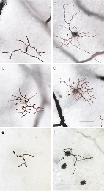
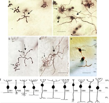
Giant bipolar cells were observed in all four retinal quadrants at the range of eccentricities (~2–7 mm) where Golgi-stained cells were found. They were easily distinguished from other bipolar cell types by their very large and sparsely branched dendritic tree and axonal stratification in the inner half of the IPL. The photomicrographs of Fig. 1 show a giant bipolar cell (Fig. 1a and 1b) and the other two inner stratifying bipolar cell types with large dendritic fields, the DB6 cell (Fig. 1c and 1d), and the blue cone bipolar (Fig. 1e and 1f). The giant bipolar’s dendritic tree is larger than that of either the DB6 or the blue cone bipolar and more sparsely branched than the DB6. Whereas the axons of the DB6 and the blue cone bipolar stratify close to the ganglion cell border (Boycott & Wässle, Reference Boycott and Wässle1991; Kouyama & Marshak, Reference Kouyama and Marshak1992), the giant bipolar’s axons costratify with the DB4 cell near the center of the IPL (Fig. 2). Examples of two giant bipolars (large arrows) with neighboring DB4 cells (small arrows) are shown in the photomicrographs of Fig. 2a–2d. The axons of both cell types are in focus at the same depth in the IPL (Fig. 2a and 2c). In the vertical section of Fig. 2e, taken from Golgi-stained whole-mount retina (see Materials and Methods), the axons of a giant cell are shown stratifying just inner to the center of the IPL. Hence, the giant cell is expected to be an ON bipolar cell. Measurement of axon depth in the IPL from whole-mount retina (see Materials and Methods) for 27 giant cells gave a mean ± s.d. of 57 ± 2.6%. The schematic of Fig. 2f is adapted from Boycott and Wässle (Reference Boycott and Wässle1991) to include the giant bipolar cell, shown stratifying at the same depth as the DB4 cell.
Photomicrographs of bipolar cells in Golgi-stained whole-mount macaque retina. Axons (a) and dendrites (b) of a giant bipolar cell located at 4.0 mm eccentricity in temporal retina. Axonal field diameter = 38 μm; dendritic field diameter = 52 μm; soma diameter = 7 μm. Axons (c) and dendrites (d) of a DB6 bipolar cell at 4.4 mm in temporal retina. Axonal field diameter = 39 μm; dendritic field diameter = 39 μm; soma diameter = 7 μm. Axons (e) and dendrites (f) of a blue cone bipolar cell at 6.4 mm temporal retina. Axonal diameter = 22 μm; dendritic field diameter = 30 μm; soma diameter = 8 μm. Arrows in (b), (d), and (f) indicate cell bodies. Scale bars = 20 μm.

Axonal stratification of the giant bipolar cell. (a) Axons of a giant bipolar (large arrow) and a DB4 bipolar (small arrow) are costratified in the inner IPL. (b) Focus is shifted to the outer plexiform layer (OPL) on the dendrites of the same cells shown in (a). Cells were located at 5.9 mm nasal retina. (c) Costratification of the axons of another giant bipolar (large arrow) and DB4 bipolar (small arrow). (d) Dendrites of the same cells shown in (b), located at 5.1 mm inferior retina. (e) Vertical section taken from Golgi-stained whole-mount retina. Arrow indicates the cell body of a giant bipolar cell whose axons stratify in the inner half of the IPL. Arrowhead indicates a blood vessel passing through the plane of the section. Scale bars = 20 μm. (f) Schematic representation of bipolar cell stratification adapted from Boycott and Wässle (Reference Boycott and Wässle1991). The giant cell (GB) is shown stratifying at the same level in the IPL as the DB4 bipolar. BB, blue cone bipolar; FMB, flat midget bipolar; IMB, invaginating midget bipolar; RB, rod bipolar.

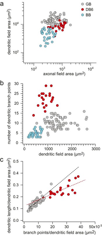
To quantify the differences in axonal and dendritic morphology between the giant bipolar, the DB6, and the blue cone bipolar, we plotted dendritic field area as a function of axonal field area for all three cell types (Fig. 3a). Although each cell type individually forms a tight cluster, the clusters are not well separated based on these parameters. The three cell types do, however, form discrete clusters based on the sparseness of their dendritic arbors, as shown in Fig. 3b, where the number of dendritic branch points is plotted as a function of dendritic field area. Fig. 3c compares dendritic sparseness of the giant bipolar and the DB6 in a plot of total dendritic length per dendritic field area against dendritic branch points per dendritic field area. The giant bipolars cluster falls to the lower left of the DB6 cluster, demonstrating that the giant bipolar has fewer branch points and lower total dendritic length per area than the DB6. The slope for each of the linear fits (giant bipolar, black dashed line; DB6, red dashed line) represents the average dendritic length per branch point and shows that the giant bipolar, with a steeper slope, tends to have longer branches than the DB6. In summary, as is apparent from the morphology, the giant bipolar has fewer longer individual dendrites, but less total dendrite, than the DB6.
Scatter plots of the axonal and dendritic field area and dendritic branch points of the giant bipolar [GB; gray circles; n = 69 in (a) and (b); n = 57 in (c)]), the DB6 [red circles; n = 21 in (a) and (b); n = 19 in (c)], and the blue cone bipolar [BB; blue circles; n = 29 in (a) and (b)] over a range of eccentricities from 2 to 7 mm from the fovea. (a) Dendritic field area plotted as a function of axonal field area. The clusters formed by each cell type are not well separated based on these parameters. (b) The number of dendritic branch points plotted as a function of dendritic field area. The three cell types form discrete clusters based on the sparseness of their dendritic trees. (c) Total dendritic length per dendritic field area plotted as a function of the number of dendritic branch points per dendritic field area for the giant and the DB6 cells. The slope of the linear fits (giant cells, black dashed line; DB6 cells, red dashed line) represents the average dendritic length per branch point. The giant bipolar has fewer longer individual dendrites, but less total dendrite, than the DB6.

Mean axonal field and dendritic field area, number of branch points, and soma area for the giant bipolar, DB6, and blue cone bipolar are summarized in Table 1. Whereas the DB6 and the blue cone bipolar each have dendritic fields similar in size to their axonal fields, the giant bipolar’s dendritic field is on average more than twice the size of its axonal field. Its soma is also smaller than that of either the DB6 or the blue cone bipolar. Also included in Table 1 is an estimate of giant bipolar density. Density was determined by assuming a coverage of 1 and dividing the coverage by the mean dendritic field area for five giant bipolars located at an eccentricity of ~4 mm in temporal retina and four cells in nasal retina that when adjusted for temporal equivalency (Rodieck & Watanabe, Reference Rodieck and Watanabe1993) had an eccentricity of ~4 mm. The density for DB6 cells was taken from Chan et al. (Reference Chan, Martin and Grünert2001; Fig. 4) for an eccentricity of ~4 mm temporal retina. The density for blue cone bipolars cells is from Kouyama and Marshak (Reference Kouyama and Marshak1992; Fig. 7) for an eccentricity of ~20 deg (4 mm) in temporal retina. Based on the estimated density, giant bipolars comprise ~2.8% of total cone bipolar cells (total cone bipolar cell density from Martin & Grünert, Reference Martin and Grünert1992; Fig. 5 for 4 mm eccentricity, temporal retina).
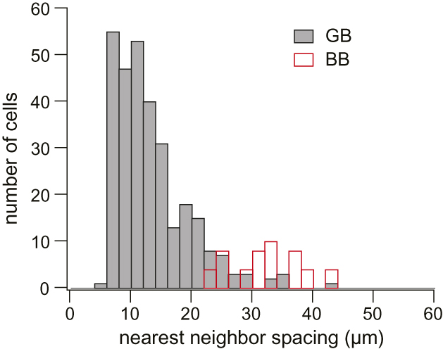
Histogram of nearest neighbor distance of cone contacts for 36 giant cells (GB; solid gray bars) (total contacts, n = 300) and 12 blue cone bipolar cells (BB; open red bars) (total contacts, n = 25). For giant cells, each dendritic tip was considered a cone contact unless it was within the average cone pedicle diameter of a neighboring dendritic tip, in which case they were together considered a single contact (see Results). S-cone spacing was estimated by measuring the nearest neighbor spacing for the dendritic terminal of blue cone bipolars. The distribution for the giant bipolar is shifted to the left of that for the blue cone bipolar. While the possibility of giant bipolars contacting S cones cannot be ruled out, they do not do so exclusively.

Photoreceptor contacts of the giant bipolar cell. (a) Photomicrograph of the axons of a giant bipolar cell in the IPL (arrowhead). Arrows indicate the axons of three invaginating midget bipolars that appear out of focus because these cells stratify closer to the ganglion cell layer than the giant bipolar. (b) Same location as in (a) with the focus shifted to the outer plexiform layer. Two giant cell dendrites can be seen contacting the same cones as two of the invaginating midget bipolars (arrows). The invaginating midget bipolar on the left has a two-headed dendritic tree. The giant cell dendrite terminates on the lower and smaller of the midget bipolar’s dendritic tufts. The cells were located at 5.1 mm eccentricity in nasal retina. (c) Tracings of a giant cell (GB; red), a blue cone bipolar (BB), and an invaginating midget bipolar (IMB) located at 4.7 mm eccentricity in inferior retina. The terminal dendrites of the midget bipolar along with two of the dendritic terminals of the blue cone bipolar are indicated with open circles. The giant cell dendrite on the far right contacts the same cone as the midget bipolar (large arrow), but it appears to bypass the two S cones within its dendritic field that are contacted by the neighboring blue cone bipolar (small arrows, blue circles). Scale bars = 20 μm.

Axonal and dendritic field area, soma area, number of branch points, and density for giant, DB6 and blue cone bipolar cells

Photoreceptor contacts
The sparseness of the giant cell’s dendritic tree indicates that it does not contact every cone in its field and that it may make selective contacts similar to those of the blue cone bipolar (Kouyama & Marshak, Reference Kouyama and Marshak1992). We investigated whether the giant bipolar also exclusively contacts S cones by measuring the nearest neighbor distance between the cone contacts of individual giant bipolars and comparing this to an estimate of S-cone spacing at the same eccentricity.
For giant bipolars, each dendritic tip was counted as an individual cone contact unless it was within the average cone pedicle diameter of a neighboring dendritic tip, in which case they were considered to contact the same pedicle. Since the cone pedicles themselves were not visible in our material, pedicle diameter was estimated by measuring the diameter of stained terminal aggregates of H1 horizontal cells and invaginating midget bipolars across their widest points. Estimated pedicle diameter was approximately equal to the cone inner segment diameter for cells at the same eccentricity (mean ± s.d. cone inner segment diameter = 6.3 ± 0.2 μm, n = 30; mean ± s.d. estimated pedicle diameter = 6.6 ± 0.9 μm, n = 151, for ~5 to 7 mm nasal retina). The distance from each cone contact to its nearest neighbor for 36 giant cells at 5–7 mm nasal retina was 13.3 ± 6.1 μm (mean ± s.d.).
S-cone spacing was estimated by measuring the nearest neighbor spacing for the terminal aggregates of blue cone bipolars in which all the cell’s dendrites ended in distinct clusters. This reduced the possibility of including “blind” dendrites that end without making S-cone contacts (Mariani, Reference Mariani1984; Kouyama & Marshak, Reference Kouyama and Marshak1992). The distance between terminal aggregates for blue cone bipolars at 5–7 mm nasal retina was 32.3 ± 5.8 μm (mean ± s.d.; n = 12).
The histogram of Fig. 4 shows the distribution of nearest neighbor spacing of cone contacts for giant and blue cone bipolars. The distribution for the giant bipolars is centered to the left of that for the blue cone bipolars, indicating that although the giant bipolar may make S-cone contacts, it does not do so exclusively.
In the photomicrographs of Fig. 5a and 5b, a giant bipolar cell (arrowhead) is shown contacting the same cones as each of two nearby invaginating midget bipolar cells (arrows). The tracing in Fig. 5c shows another giant cell also contacting the same cone as a neighboring invaginating midget bipolar (large arrow) while “bypassing” S cones being contacted by a nearby blue cone bipolar (small arrows). Although one dendrite of the giant bipolar passes across a terminal cluster of the blue cone bipolar (middle arrow), it does not appear to send a terminal dendrite to contact the same cone pedicle. Blue cone bipolars, by contrast, almost never “bypass” S cones in this manner (Kouyama & Marshak, Reference Kouyama and Marshak1992).
Percentage of cones contacted
We further examined the sparse branching of the giant cell’s dendritic tree by estimating the percentage of cones contacted per total cones in its dendritic field. The mosaic of cone inner segments was often visible above the stained bipolar cells and was used to estimate the total number of cones in an individual giant bipolar’s dendritic field. At the eccentricity where our cells were located, there is a small Henle fiber shift between cone inner segments and pedicles (Boycott et al., Reference Boycott, Hopkins and Sperling1987; Perry & Cowey, Reference Perry and Cowey1988). Given the regularity of the cone inner segment mosaic, we questioned whether the shift would affect our estimates. We tested this for one giant bipolar by shifting the inner segment mosaic according to the apparent displacement between spherules and inner segments of three stained rods in or near the giant bipolar’s dendritic field (after Boycott & Wässle, Reference Boycott and Wässle1991). Since correcting for the shift did not change our estimate of the number of cones, we did not correct for the Henle fiber shift in subsequent calculations.
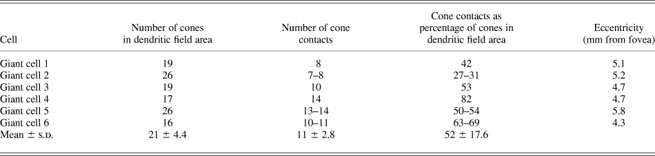
The cell tracings in Fig. 6 illustrate the method for determining the number of cones contacted by an individual cell for two giant cells (Fig. 6a and 6b) and one DB6 cell (Fig. 6c). Circles on the left show the mosaic of cone inner segments overlying each cell. The cell’s dendritic field is defined by the convex polygon around the outermost dendrites, and cones within or abutting the dendritic field are shown in gray. The circles on the right represent cone pedicles contacted by the cell, which were assumed to be the same size as the inner segments in the field (see above). Application of this method to the DB6 cell confirms that it contacts nearly all the cones in its dendritic field, though occasionally “holes” in the DB6 dendritic network have been observed (Hopkins & Boycott, Reference Hopkins and Boycott1997; Lee et al., Reference Lee, Jusuf and Grunert2004). In contrast, the two giant cells shown in Fig. 6 contacted less than half the cones in their dendritic fields. The percentage of cones contacted for the giant cells in Fig. 6a and 6b are shown in Table 2 as giant bipolars 1 and 2, respectively. The percentage of cones contacted for four other giant bipolars is also shown in Table 2. Where the spacing of adjacent dendrites was ambiguous as to whether they were contacting one cone or two, both values are given. The mean ± s.d. for the percentage of cones contacted within the cells’ dendritic fields was 52 ± 17.6% (n = 6).
Illustration of the method for determining the percentage of cones a giant cell contacts within its dendritic field. (a and b) Tracings of two giant cells located at 5.1 mm nasal (a; same cell as in Fig. 5b) and 5.2 mm temporal retina (b). Circles on the left show the mosaic of cone inner segments overlying the cells; shaded circles denote cones counted as being within the cells’ dendritic field, defined by the convex polygon around the dendrites. Circles on the right represent cone pedicles and indicate cones contacted by the cell. The giant bipolars contact less than half the cones within their dendritic fields. (c) Tracing of a DB6 cell at 5.2 mm nasal retina. Cone placement and contacts as in (a) and (b). Unlike the giant cells, the DB6 cell contacts all the cones within its dendritic field. Scale bar = 20 μm.

The percentage of cones contacted by individual giant cells

Dendritic interaction
The wide range in the percentage of cones contacted by an individual giant cell (27–82%; see Table 2) could be explained by dendritic overlap between neighboring cells. Assuming such overlap, the percentage of contacted cones could be as high as 100%. While the staining in our material did not reveal extensive patches of the giant bipolar mosaic, neighboring pairs of giant bipolars were observed. The tracings in Fig. 7a–7c show three pairs of neighboring giant bipolars. There is virtually no dendritic overlap between the pairs, indicating that giant bipolars’ dendritic fields have a coverage of 1. In other words, the giant bipolar cells are likely to tile the retina without overlap, as has been shown for the primate DB6 (Chan et al., Reference Chan, Martin and Grünert2001) and blue cone bipolar cell (Boycott & Wässle, Reference Boycott and Wässle1991; Kouyama & Marshak, Reference Kouyama and Marshak1992) as well as for all mouse bipolar types (Wässle et al. Reference Wässle, Puller, Muller and Haverkamp2009).
Dendritic overlap and interactions of giant bipolar cells. (a–c) Tracings of three pairs of neighboring giant cells from 6.7 mm inferior (a), 5.9 mm nasal (b), and 4.7 mm inferior (c) retina. There is virtually no dendritic overlap between neighboring cells, ruling out the possibility that the giant cell mosaic as a whole contacts all the cones within the area. The open circles indicate where the dendrites of cells converge onto the same cone pedicle. (d and e) Tracings of two giant cells from 5.1 mm nasal (d; same cell as in Fig. 5b & 6a) and 5.3 mm inferior (e) retina. The open circles indicate where dendrites within the individual cell’s dendritic tree converge onto a single cone pedicle.

A coverage of ~1 suggests that the density of contacts made at any point across the entire mosaic of giant bipolars really is as variable as the range of percentages indicates. It is possible that the giant bipolar makes nonspecific contacts with a variable percentage of total cones in its field. As the tracings in Fig. 7 illustrate, however, dendrites from neighboring cells often converge at the same cone pedicle (circles; Fig. 7a–7c). Dendritic convergence has also been observed for single cells, as illustrated by the circled dendritic tips in the tracings of the two giant bipolars shown in Fig. 7d and 7e. If the giant bipolar contacted cones indiscriminately, dendritic convergence at the same cone pedicle would be rare, and especially so because it has so few dendrites. Frequent observation of such convergence strongly suggests the giant bipolar cell selectively targets a distinct subset of cones.
Discussion
The capricious nature of the Golgi stain can sometimes result in an incomplete or inaccurate account of retinal anatomy, misleading investigators attempting a detailed analysis. An example is Mariani’s identification of Golgi-impregnated “biplexiform ganglion cells” (Polyak, Reference Polyak1941; Mariani, Reference Mariani1982; Wässle et al., Reference Wässle, Dacey, Haun, Haverkamp, Grünert and Boycott2000), which were later identified as displaced H2 cells (Wässle et al., Reference Wässle, Dacey, Haun, Haverkamp, Grünert and Boycott2000). We are aware that a recurrent anatomical abnormality will sometimes be misclassified as a new cell “type,” but this does not appear to be the case in the present study. In our Golgi-stained retinas, we were able to reliably identify all previously recognized bipolar cell types and confirm their axonal stratification depth as well as their dendritic and axonal morphology, and our retinas provided a large sample of well-stained giant cells for quantitative analysis and direct comparison with other bipolar types in the same material.
Our results provide the first detailed description of the giant bipolar cell type in the monkey retina. Bipolar cells described as “giant,” however, have been previously observed. Polyak (Reference Polyak1941) briefly described a large bipolar cell in Golgi-stained monkey retina, which he referred to as g-type. Polyak gave no detailed information on these cells because he concluded they were “probably merely a freakish local modification” of a type of diffuse cell (his “brush” or “flat” bipolar cells). Of the four g-type cells Polyak illustrated, two cells (Figs. 55 and 93) have the characteristic large dendritic field and approximately the same axonal stratification depth as the giant bipolars described here. Mariani (Reference Mariani1983) described giant bistratified bipolar cells with a large axonal arborization in Polyak’s layer 7a and a smaller one in layer 7d. We did not, however, observe any giant cells with bistratified axonal arbors.
In their study of bipolar cell types in Golgi-stained macaque retina, Boycott and Wässle (Reference Boycott and Wässle1991) did not observe bistratified giant cells, but they did see cells “with rather large dendritic fields” (Fig. 10d). These cells did not fit the description for any of the six types of diffuse cells they described and the authors felt that they may have represented an additional cell type, but the overall quality of the staining of the cells did not permit a detailed characterization. In a plot of axonal versus dendritic field area Rodieck (Reference Rodieck and Steklis1988; Fig. 22) identified a “giant” cluster with axonal and dendritic field areas within the range of the giant cells described here, though it is unclear whether his cluster included DB6 cells, which also have large dendritic fields relative to the other diffuse bipolar cell types.
It is likely that Polyak’s g-type, Rodieck’s giant cluster, and the large cells observed by Boycott and Wässle all correspond to the giant bipolars described in this paper. In a Golgi study of human retina, Kolb et al. (Reference Kolb, Linberg and Fisher1992) also observed several examples of a wide-field bipolar type, their GBb cell, that stratified at a similar depth in the IPL as our giant bipolars. As Boycott and Wässle noted, giant bipolar cells have large dendritic fields and a low density, which could explain why they have rarely been observed previously in primate retina.
Bipolar cells with large dendritic fields have also been described in nonprimate mammalian retina. In cat retina, Famiglietti (Reference Famiglietti1981) described an inner stratifying wide-field bipolar cell that stratified close to the middle of the IPL, similar to the stratification of the our giant bipolar. Pourcho and Goebel (Reference Pourcho and Goebel1987) also described a bipolar cell in cat retina, the CBb5, with a large sparse dendritic tree, thick dendrites, and an inner stratifying axonal field smaller than its dendritic field. Although the CBb5’s axonal arbor appeared to be more broadly stratified than our giant bipolar, the overall dendritic and axonal morphology was very similar to that of the giant bipolar. It is possible that Famiglietti’s wide field bipolar and Pourcho and Goebel’s CBb5 cell may represent the cat correlate of our monkey giant bipolar.
Of the cell types included in a complete classification scheme for mouse bipolars, the types 5a and 5b have axons that stratify at a level in the IPL similar to the stratification depth of our giant bipolars (Ghosh et al., Reference Ghosh, Bujan, Haverkamp, Feigenspan and Wassle2004; Wässle et al., Reference Wässle, Puller, Muller and Haverkamp2009). While their dendritic and axonal morphology have not been investigated and their cone contacts are unknown, it is possible that one of these types may represent the mouse correlate of the giant bipolar.
Analysis of the giant bipolar’s dendritic morphology and cone contacts suggests that it does not contact every cone in its field, introducing the functionally relevant question of which cones it does contact. The values for nearest neighbor distance between cone contacts were too low for the giant bipolar to be contacting exclusively S cones (Fig. 4). This is further supported by examples of the giant bipolar contacting the same cone pedicles as invaginating midget bipolars (Fig. 5). The percentage of cones contacted (mean ± s.d. = 52 ± 17.6; n = 6) also indicates that they do not exclusively contact S cones, which account for only ~10% of all cones (de Monasterio et al., Reference de Monasterio, Schein and McCrane1981, Reference de Monasterio, McCrane, Newlander and Schein1985).
The wide range for percentage of cones contacted and observation of frequent dendritic convergence at the same cone pedicle together suggest that the giant bipolar is targeting a specific subpopulation of cones that itself has a highly variable local density and comprises ~50% of all cones. The lack of dendritic overlap seen in pairs of neighboring cells indicates that giant bipolars do not compensate for the variable percentage of cones contacted with a variable degree of overlap; instead, the percentage of cones contacted by the mosaic as a whole varies depending on location. This description is consistent with that of the L and M cone submosaics, which each comprise about half the total cones excluding S cones and tend to cluster (Packer et al., Reference Packer, Williams and Bensinger1996) such that locally they can comprise a percentage as variable as that of the giant’s cone contacts. Because of L and M cone clustering (Roorda et al., Reference Roorda, Metha, Lennie and Williams2001), a bipolar cell that makes exclusive L or M contacts would be expected to show “clustering” of its cone contacts; the cell tracing in Fig. 6b is an example of this. Although the percentage of cones contacted also falls into the range that would be expected if the giant bipolar contacted S cones along with L or M cones, giant bipolar dendrites have been seen bypassing S cones (Fig. 5), which would be unlikely if they regularly contacted S cones in addition to L or M cones.
The sparseness of the giant bipolar’s cone contacts and the possibility of the cell selectively contacting a subset of the L and M cones raises the intriguing question of whether the giant bipolar plays a role in color vision. Such a role, however, would only apply to the trichromatic primate retina. In the nonprimate dichromatic retina, low-density cone subpopulations identified by specific protein expression have been described (Balse et al., Reference Balse, Tessier, Forster, Roux, Sahel and Picaud2006; Wässle et al., Reference Wässle, Regus-Leidig and Haverkamp2006), suggesting the possibility of other, nonchromatic, roles for the giant bipolar cell. Further physiological analysis will be needed to address these questions and to form a complete characterization of the giant bipolar’s function within the retina.
Acknowledgments
This work was supported by the National Primate Research Center at the University of Washington (RR00166) and National Institutes of Health Grants (EY06678 to D.M.D.) and (EY01730) (Vision Research Center Core). We thank Christian Puller for his many helpful suggestions and editorial assistance.