


1. Introduction
The particle-laden thermal convections are ubiquitous in nature (Jellinek & Kerr Reference Jellinek and Kerr2001; Shaw Reference Shaw2003) and industrial contexts (Hunt Reference Hunt1991; Pouransari & Mani Reference Pouransari and Mani2017). The dynamic coupling between particles and thermal turbulence is crucial in natural or engineering processes, as the particle-laden turbulence can change the dynamics of the systems (Elghobashi Reference Elghobashi1994; Balachandar & Eaton Reference Balachandar and Eaton2010). In addition, the settling and preferential concentration of particles are also strongly correlated with the coupling mechanism (Hanna Reference Hanna1969; Kok et al. Reference Kok, Parteli, Michaels and Karam2012; Davis et al. Reference Davis, Jafarian, Chinnici, Saw and Nathan2019).
The particle-laden flows can be classified as being either dense or dilute according to whether the particle–particle collision is important (Crowe Reference Crowe1982; Elghobashi Reference Elghobashi1994). The classification is realized by a volume fraction of particles  $(\varPhi _{V})$. When
 $\varPhi _{V}$ is larger than
 $10^{-3}$, the interaction between particles (such as collision, agglomeration and breakup) are important, and this regime termed the dense dispersion regime is described as four-way coupled. When
 $\varPhi _{V}$ is below
 $10^{-3}$, the dilute dispersion regime is encountered and the flow is either one-way
 $(\varPhi _{V} \le 10^{-6})$ or two-way
 $(10^{-6} \le \varPhi _{V} \le 10^{-3})$ coupled (Elghobashi Reference Elghobashi1994; Balachandar & Eaton Reference Balachandar and Eaton2010). From a numerical perspective, there are a few alternative approaches in terms of volume fraction, relative particle size and mass loading, such as the fully resolved approach, Lagrangian point-particle approach, Eulerian approaches, equilibrium Eulerian approaches and dusty gas approaches, which suit a range of different volume fraction, particle sizes and particle response times (Elghobashi Reference Elghobashi1991, Reference Elghobashi1994; Crowe, Troutt & Chung Reference Crowe, Troutt and Chung1996; Loth Reference Loth2000; Guha Reference Guha2008; Balachandar & Eaton Reference Balachandar and Eaton2010). We are interested in microscale inertial particle-laden flow which is a distinctive subject for the investigation of the modulation of turbulent flow as well as the kinematic and dynamical behaviours of particles.
In the one-way coupling regime, the particles have a negligible effect on turbulence. The settling and preferential concentration of particles are well investigated for this regime, and the centrifugal effect, sweep-stick mechanism, and turbophoresis are well established (Reeks Reference Reeks1983; Maxey Reference Maxey1987; Squires & Eaton Reference Squires and Eaton1991; Wang & Maxey Reference Wang and Maxey1993; Puragliesi et al. Reference Puragliesi, Dehbi, Leriche, Soldati and Deville2011; Bec, Homann & Ray Reference Bec, Homann and Ray2014). In the two-way coupling regime, the influence of the dispersed phase on the carrier-phase dynamics cannot be ignored and the turbulent dynamics can be altered (Elghobashi Reference Elghobashi1994; Balachandar & Eaton Reference Balachandar and Eaton2010). For instance, it is found that particles transfer their momentum to the small-scale flow structure, and accompanied an increase of the viscous dissipation in isotropic turbulence (Elghobashi & Truesdell Reference Elghobashi and Truesdell1993; Boivin, Simonin & Squires Reference Boivin, Simonin and Squires1998; Druzhinin & Elghobashi Reference Druzhinin and Elghobashi1999). What is more, the settling of particles makes turbulent energy redistribute from the horizontal to the vertical direction (Ferrante & Elghobashi Reference Ferrante and Elghobashi2003). For turbulent shear flows, Kulick, Fessler & Eaton (Reference Kulick, Fessler and Eaton1994) experimentally found that the turbulence is attenuated under the effect of small Stokes number particles. Ahmed & Elghobashi (Reference Ahmed and Elghobashi2000) numerically found that particles increase the local velocity gradients which in turn increase the turbulence energy dissipation rate.
Besides the influence on the velocity field, particles can also play an important role in heat transfer. Pouransari & Mani (Reference Pouransari and Mani2018) showed that the particle Stokes number and the heat-mixing parameter have the most significant effect on particle-to-gas heat transfer in particle-laden isotropic turbulence. Moreover, the temperature statistics and the heat transfer mechanism are well investigated in particle-laden turbulent homogeneous shear flow and turbulent channel flow (Shotorban, Mashayek & Pandya Reference Shotorban, Mashayek and Pandya2003; Zonta, Marchioli & Soldati Reference Zonta, Marchioli and Soldati2008; Liu et al. Reference Liu, Tang, Dong and Shen2018). Carbone, Bragg & Iovieno (Reference Carbone, Bragg and Iovieno2019) further characterize the multiscale thermal properties of the particles, and their contribution to the properties of the fluid temperature field. In most previous studies, the temperature is treated as a passive scalar. However, thermal buoyancy is usually the driving force and cannot be neglected. Gereltbyamba & Lee (Reference Gereltbyamba and Lee2019) recently found that both momentum coupling and thermal coupling suppress heat transfer more significantly than that of momentum coupling only in a three-dimensional (3-D) differentially heated cavity (known as DHC). The single-phase Rayleigh–Bénard (RB) convection, which is a paradigmatic example used to study the buoyancy-driven fluid flow, has been extensively investigated in the recent decades (Ahlers, Grossmann & Lohse Reference Ahlers, Grossmann and Lohse2009; Lohse & Xia Reference Lohse and Xia2010; Wang, Zhou & Sun Reference Wang, Zhou and Sun2020; Yang et al. Reference Yang, Zhang, Jin, Dong, Wang and Zhou2021). As for the RB convection laden with micro isothermal inertial particles, Oresta & Prosperetti (Reference Oresta and Prosperetti2013) found that mechanical coupling plays a greater role in the increase of the Nusselt number (Nu) than the thermal coupling in a cylindrical cell. However, Park, O'Keefe & Richter (Reference Park, O'Keefe and Richter2018) studied the RB convection laden with non-isothermal particles in a 3-Dl rectangular cell, they found that thermal coupling overwhelms the momentum coupling in enhancing Nu. Xu et al. (Reference Xu, Tao, Shi and Xi2020) recently studied the particle transport and deposition in a two-dimensional (2-D) square RB convection cell in a one-way coupling regime, and they defined three deposition states. In addition, the radiative heating of particles can also result in the formation of buoyant plumes, leading to the modulation of the flow field. Zamansky et al. (Reference Zamansky, Coletti, Massot and Mani2014, Reference Zamansky, Coletti, Massot and Mani2016) numerically studied the turbulence induced by heated inertial particles; they found the dependence of velocity and temperature distribution as well as intermittency on the Stokes number. Frankel et al. (Reference Frankel, Pouransari, Coletti and Mani2016) numerically found that the heated inertial particles reduce turbulent kinetic energy at low radiation levels, and increase it at high radiation levels in homogeneous turbulence.
Furthermore, the distribution, transportation and settling of particles strongly affect the interphase coupling mechanism. The kinematic behaviour of particles in a two-way coupling regime is similar to that in a one-way coupling regime. Monchaux, Bourgoin & Cartellier (Reference Monchaux, Bourgoin and Cartellier2010) identified the particle clusters by using Voronoï diagram analysis. Oresta & Prosperetti (Reference Oresta and Prosperetti2013) investigated the distribution of isothermal particles in the gravity-oriented direction in RB convection in a cylindrical container. Gereltbyamba & Lee (Reference Gereltbyamba and Lee2019) found that there are different transportation regimes of particles in a 3-D differentially heated cavity. Frankel et al. (Reference Frankel, Pouransari, Coletti and Mani2016) found that the hot plumes shed from a heated particle can reduce the mean particle settling velocities in homogeneous turbulence.
The coupling mechanisms are important for turbulence modulation and the behaviour of particles. We note that there is still a lack of systematic studies on this issue for the particle-laden RB turbulent convection. What is more, to our knowledge, there is no theoretical description for the particle-induced energy in the coupling system. Here we focus on the interphase coupling as well as its effects on the modulation of flow field for buoyancy-driven turbulent flow laden with microscale particles; besides, we also investigated the settling law and preferential concentration of particles. The remainder of this paper is organized as follows. In § 2, we briefly describe the mathematical model and numerical procedure. Results and discussion are presented in § 3, and it can be divided into four parts. We describe the alteration of global features in § 3.1 and discuss the modulation of the scaling of Nu and Re in § 3.2. In § 3.3, we derive the exact relation for the kinetic energy dissipation in particle-laden RB convection system, and further analyse the effects of particle-induced kinetic energy. Section 3.4.1 and § 3.4.2 discuss the settling and preferential concentration of particle. Finally, we give a conclusion for this work in § 4.
2. Mathematical model and numerical procedure
We study the RB convection laden with micro isothermal inertial particles. The governing equations of the flow field is under the simplification of the Oberbeck–Boussineq approximation (Landau & Lifshitz Reference Landau and Lifshitz1987; Boussinesq Reference Boussinesq1903). The volume occupied by the particles is very small, so the fluid continuity equation retains the standard incompressible form, and we write the momentum equations and energy equation, in dimensionless form, as
 $$\begin{gather} \boldsymbol{\nabla}\boldsymbol{\cdot}\boldsymbol{u} = 0, \end{gather}$$
 $$\begin{gather}\frac{{\partial}\boldsymbol{u} }{{\partial} t}+(\boldsymbol{u} \boldsymbol{\cdot}\boldsymbol{\nabla})\boldsymbol{u}={-}\boldsymbol{\nabla} p+\frac{1}{\sqrt {Ra/Pr}}\nabla^{2}\boldsymbol{u}+\theta\boldsymbol{e}_2+\boldsymbol{F}, \end{gather}$$
 $$\begin{gather}\frac{{\partial}{\theta} }{{\partial} t}+(\boldsymbol{u}\boldsymbol{\cdot}\boldsymbol{\nabla})\theta=\frac{1}{\sqrt {Ra\boldsymbol{\cdot} Pr}}\nabla^{2}{\theta}, \end{gather}$$
here,  $\boldsymbol {u}$,
 $\theta$ and
 ${p}$ are, respectively, the velocity, temperature and kinematic pressure, and
 ${\boldsymbol {e}_2}$ is the vertical upward unit vector. The term
 $\boldsymbol {F}$ represents the momentum feedback of the particles, which will be described later. The equations (2.1)–(2.3) are normalized by the cell height
 ${H}$, the temperature difference
 $\varDelta$ across the fluid layer of height
 ${H}$, and characteristic velocity
 $u^*=\sqrt {\beta g\varDelta {H}}$, where
 $\beta$ is the thermal expansion coefficient and
 $g$ is the acceleration due to gravity. The Rayleigh number and Prandtl number are defined as
 ${Ra}={\beta g\varDelta {H}^3}/{(\kappa \nu )}$ and
 ${Pr}=\nu /\kappa$, with
 $\kappa$,
 $\nu$ being the thermal diffusivity and kinematic viscosity of the working fluid, respectively (Ahlers et al. Reference Ahlers, Grossmann and Lohse2009; Lohse & Xia Reference Lohse and Xia2010; Chillà & Schumacher Reference Chillà and Schumacher2012; Xia Reference Xia2013). Moreover, there are two response parameters, Nusselt number
 $Nu$ and Reynolds number
 $Re$, which are calculated as
 $Nu=\sqrt {RaPr}\langle v\theta \rangle -\langle { {\partial } \theta }/{ {\partial } z}\rangle$ and
 $Re=U_{rms}\sqrt {Ra/Pr}$, respectively, here
 $u$ is the horizontal velocity,
 $v$ is the vertical velocity and
 $U_{rms}=\sqrt {\langle (u^2+v^2)\rangle }$.
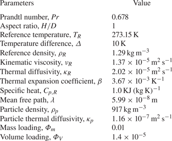
In this work, the volume fraction of the particle is sufficiently low to neglect particle–particle interaction (Elghobashi Reference Elghobashi1994, Reference Elghobashi2019), the density of particles is much higher than that of the fluid, and the particle diameters are small compared with the Kolmogorov scale of turbulence. All the constant properties of the simulations are shown in table 1; we can see that  ${Pr}=0.678$, a value appropriate, for example, for air at
 $0\,^\circ$C and the particle physical properties are close to those of ice at
 $0\,^\circ$C. Under the above assumptions the major forces acting on particles are Stokes drag and gravity (Elghobashi & Truesdell Reference Elghobashi and Truesdell1992; Guha Reference Guha2008; Balachandar & Eaton Reference Balachandar and Eaton2010). Considering that there are relatively large gradients of velocity and temperature in the system, the resulting Saffman lift (Saffman Reference Saffman1965; Mei Reference Mei1992; Cherukat, Mclaughlin & Dandy Reference Cherukat, Mclaughlin and Dandy1998; Kurose & Komori Reference Kurose and Komori1999) and thermophoresis (Talbot et al. Reference Talbot, Cheng, Schefer and Willis1980; Puragliesi et al. Reference Puragliesi, Dehbi, Leriche, Soldati and Deville2011) on particles should be taken into consideration. Therefore, we write the particle equations, in dimensionless form, as
 $$\begin{gather} \frac{\mathrm{d}\kern0.06em \boldsymbol{x}_p}{\mathrm{d} t}=\boldsymbol{u}_p, \end{gather}$$
 $$\begin{gather}\frac{\mathrm{d} \boldsymbol{u}_p}{\mathrm{d} t}={-}\frac{1}{Fr^2_p}\boldsymbol{e}_2-\frac{C_D}{St_f}(\boldsymbol{u}_p- \boldsymbol{u})+C_L[(\boldsymbol{u}-\boldsymbol{u}_p)\times\boldsymbol\omega]+C_{th} \frac{\boldsymbol{\nabla}\theta}{T_0/\varDelta+\theta}, \end{gather}$$
where  $\boldsymbol {x}_p$ and
 $\boldsymbol {u}_p$ are the particle dimensionless position and velocity, respectively. Here
 $Fr_p=\sqrt {\beta \varDelta }$ represents the ratio of inertia force of fluid to gravity of a particle. Furthermore,
 $C_D=1+0.15Re_p^{0.678}$ represents the drag correction coefficient which applies when the particle Reynolds number
 $Re_p=(d_p/H)|\boldsymbol {u}-\boldsymbol {u}_p|(Ra/Pr)^{1/2}$ exceeds unity, where the notation
 $|\boldsymbol {u}-\boldsymbol {u}_p|$ refers to the magnitude of the vector difference between the fluid and particle velocities,
 $d_p$ is the particle diameter and the fluid velocity
 $\boldsymbol {u}$ at the particle location are interpolated using fourth-order Lagrange interpolation. The particle Stokes number based on the integral time scale is given by
 $St_f=(1/18)(\rho _p/\rho _R)(d_p/H)^2(Ra/Pr)^{1/2}$ which represents the inertia of a particle in the flow field, where
 $\rho _p$ and
 $\rho _R$ are, respectively, the particle density and the fluid density. Here
 $C_L$ and
 $C_{th}$ are Saffman lift and thermophoresis coefficients, respectively (Talbot et al. Reference Talbot, Cheng, Schefer and Willis1980; Mei Reference Mei1992; Dong & Chen Reference Dong and Chen2011; Puragliesi et al. Reference Puragliesi, Dehbi, Leriche, Soldati and Deville2011).
Summary of the fluid and particle properties used in the simulation.

In this research, the volumetric particle loading is large enough to alter the turbulence structure (Elghobashi & Truesdell Reference Elghobashi and Truesdell1992) and the size of particles is far less than the Kolmogorov scale of the flow field, so the point-particle model applies. Note that we have ignored the change of particle temperature and corresponding two-way thermal coupling, because the temperature difference between fluid and particles is rather small and heat transfer between them is negligible. Also, the resident time of particles is rather small, we therefore consider particles as the isothermal case. Here  $\boldsymbol {F}$ represents the total force exerted on the fluid by the point-particle in each fluid cell (Oresta & Prosperetti Reference Oresta and Prosperetti2013; Liu et al. Reference Liu, Tang, Dong and Shen2018). Normalized by the mass of the fluid in each cell,
 $\boldsymbol {F}$ is expressed as
 \begin{equation} \boldsymbol{F}={-}\frac{\rm \pi}{6}\frac{\rho_p}{\rho_R}\frac{d_P^3}{V}\sum_{j=1}^{N} \left({\frac{\mathrm{d} \boldsymbol{u}_p}{\mathrm{d} t}-\left(-\frac{1}{Fr_p^2} \boldsymbol{e}_2\right)}\right), \end{equation}
where  $V$ is the fluid volume of the cell and
 $N$ is the number of particles in the cell.
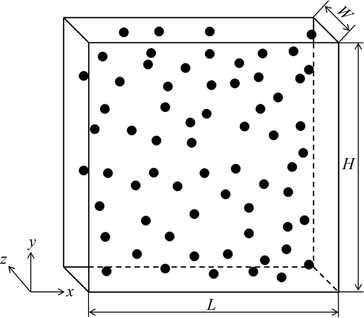
The RB convection model that we considered here is quasi-3-D, as shown in figure 1, the thickness of the cell in the  $z$-direction
 $W$ is very thin and is set as
 $H/\sqrt N_p$, and
 $N_p$ is the total number of particles. In this way, on average, a specific particle will occupy a 3-D box with sides equal to
 $H/\sqrt N_p$. In this physics model, we assume that the velocities of both the fluid and the particles in the
 $z$-direction are very small and can thus be neglected. The coupling between fluid and particle features is 3-D to some extent, while the flow characteristics tend to be generally 2-D. Consequently, a 2-D RB convection flow laden with inertial particles is considered as a model flow representative of the physical processes inherent in turbulent RB convection two phase flows. The box has height
 $H=1$ and width
 $L=1$, and no-penetration and no-slip velocity boundary conditions are applied to all four solid walls. The temperature
 $\theta$ on the two lateral walls is assumed to be adiabatic, i.e. no heat flux, while the top and bottom plates are held at constant temperatures of
 $-$0.5 and
 $+$0.5, respectively. The motivations for this approximation mainly include the following: (i) many of the important physical processes found in 3-D flows laden with inertial particles are also present in the 2-D model (Patočka, Calzavarini & Tosi Reference Patočka, Calzavarini and Tosi2020; Xu et al. Reference Xu, Tao, Shi and Xi2020); (ii) many well-cited theories for turbulent RB systems are essentially 2-D, e.g. the popular Grossmann–Lohse theory (Grossmann & Lohse Reference Grossmann and Lohse2000) and the Whitehead–Doering theory for the ultimate regime (Whitehead & Doering Reference Whitehead and Doering2011); (iii) the 2-D turbulence has been a possible application to intermediate-scale meteorological flow (Kraichnan Reference Kraichnan1967), and it can be used to better understand the physical mechanisms of 3-D convection (van der Poel, Stevens & Lohse Reference van der Poel, Stevens and Lohse2013).
Configuration of turbulent RB convection laden with inertial particles.

The governing equations (2.1)–(2.3) are discretized using a second-order central difference method. After the flow field is fully developed, particles are injected into the flow field at a random position, with their velocities set to those of the local fluid, then continue the simulation of the particle-laden flow. In the computation, Lagrangian particle tracking is employed to obtain the position and velocity of the particles. Equations of particle's evolution are advanced in time by a second-order Adams–Bashforth method (Dong & Chen Reference Dong and Chen2011). For particles, an elastic reflection is enforced at the upper wall and the two lateral walls. When a particle reaches the bottom of the cell, it is removed from the calculation and a new particle is reinjected at a random position on the top plate with the velocity equal to zero. In this study, the Prandtl number is fixed at  $Pr=0.678$, the Froude number is fixed at
 $Fr_p=0.191$, the mass loading and volume loading are fixed at 0.01 and
 $1.4\times 10^{-5}$, respectively. Three typical Stokes numbers
 $St_f=8\times 10^{-3}$,
 $St_f=2.5\times 10^{-2}$ and
 $St_f=1\times 10^{-3}$ are considered for a Rayleigh number in the range of
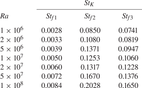
 $1\times 10^{6}\le Ra \le 1\times 10^{8}$. The Stokes numbers based on both the Kolmogorov and integral time scales of the flow are given in table 2. The coupling mechanism in the RB convection laden with inertial isothermal particles is investigated.
The Stokes number based on the Kolmogorov time scale of the flow  $St_{K}$ for the simulated cases at small
 $St_{f1}=1.0\times 10^{-3}$, medium
 $St_{f2}=8.0\times 10^{-3}$ and large
 $St_{f3}=2.5\times 10^{-2}$.

3. Results
3.1. Global flow features
The flow structures at  $Ra=10^8$ for a single-phase case and the particle-laden cases with three Stokes numbers, i.e.
 $St_f=1.0\times 0^{-3}$,
 $St_f=8.0\times 10^{-3}$ and
 $St_f=2.5\times 10^{-2}$, are shown in figure 2(a–d). A large-scale circulation (LSC) accompanied with four small secondary rolls is observed in the single-phase case in figure 2(a), the hot fluid ascends on one side and the cold fluid descends on the other side. The flow structure changes a small amount at
 $St_f=1.0\times 10^{-3}$ and
 $St_f=2.5\times 10^{-2}$, see figure 2(b) and figure 2(d). In contrast, the flow structure varies a large amount and the LSC becomes unstable at medium Stokes numbers
 $St_f=8.0\times 10^{-3}$, as plotted in figure 2(c). Such results indicate that the effect of coupling between particles and fluid is stronger for particle-laden flow with medium Stokes number. We will discuss this later through particle-induced kinetic energy analysis in § 3.3.
Typical snapshots of the instantaneous temperature field (colour) and streamlines (black lines with arrows) for  $Ra=10^8$ at
 $Pr=0.678$: (a) single-phase; (b)
 $St_f=1.0\times 10^{-3}$; (c)
 $St_f=8.0\times 10^{-3}$; (d)
 $St_f=2.5\times 10^{-2}$. Here 4 % of the total number of particles are shown for clarity.

Additionally, the distribution of particles is also given in figure 2(b–d). For  $St_f=1.0\times 10^{-3}$, there are almost no particles in the core of LSC, and the distribution of particles is nearly homogeneous in the other region, as shown in figure 2(b). As in this small Stokes number case, the inertia of the particles is small, the particles respond rapidly to the change of the surrounding flow. Due to the centrifugation effect, the particles drift outwards and spiral away from the vortex core (Maxey Reference Maxey1987). This why the inertial particles have little effect on the flow structures. For
 $St_f=2.5\times 10^{-2}$, the particle motion is mainly affected by particle inertia rather than surrounding flow, consequently, there is no remarkable correlation between the distribution of particles and the structure of eddies, and the particles seem to be distributed randomly in the flow as shown in figure 2(d). For the medium Stokes number
 $St_f=8.0\times 10^{-3}$, we can see from figure 2(c) that the distribution of particles is very non-uniform and the regions of higher particle concentration tend to appear as long, connected patches or sheets. Moreover, under the effect of inertial bias and local velocity field, the preferential sweeping of particles is relevant to the edges of the eddy and rotational zones (Wang & Maxey Reference Wang and Maxey1993). These local clusters which act on the edges of the eddy can most effectively alter the strength and the shape of the eddy as shown in figure 2(c), meanwhile, the turbulence production, distortion and dissipation become important. The local accumulation of particles is also evident for the cellular flow and has been repeatedly observed for free shear flows, such as the plane mixing layer and jet flows (Crowe, Gore & Troutt Reference Crowe, Gore and Troutt1985; Chung & Troutt Reference Chung and Troutt1988; Lázaro & Lasheras Reference Lázaro and Lasheras1992; Longmire & Eaton Reference Longmire and Eaton1992).
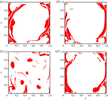
The thermal plumes are also impacted by the two-way coupling, this can be intuitively seen form the distribution of thermal field as shown in figure 2. To precisely detect thermal plumes, we follow the approach of Huang et al. (Reference Huang, Kaczorowski, Ni and Xia2013) and Zhang, Zhou & Sun (Reference Zhang, Zhou and Sun2017). A thermal plume is defined as a region where
 \begin{equation} |\theta(x,y)-\langle \theta \rangle_x|>c\theta_{rms} \quad\text{and}\quad \sqrt{RaPr}|v(x,y)\theta(x,y)|>cNu. \end{equation}
The empirical constant  $c$ is chosen to be 1.2, which is the same as that of Zhang et al. (Reference Zhang, Zhou and Sun2017). By applying the above criterion, we depict the plume regions in the figure 3 (in red). The thermal plumes are ejected from the corner of the bottom/top plate, and transported along the sidewalls for the single-phase case as shown in figure 3(a). The thermal plumes change a little at
 $St_f=1.0\times 10^{-3}$ and
 $St_f=2.5\times 10^{-2}$ as plotted in figure 3(b,d). As for
 $St_f=8.0\times 10^{-3}$ as shown in figure 3(c), the thermal plumes vary a great deal. We can see more plumes are ejected from the middle of the bottom/top plate, moreover, there are lots of plumes in the bulk region. Overall, even if there is no direct thermal interaction between the fluid and particles, the plume structure is dependent on
 $St_f$. Moreover, the variation of thermal plumes and flow structure affect the global heat transfer in the cell; we will further study the relevant
 ${\rm Nu}{\sim} {\rm Ra}$ and
 ${\rm Re}{\sim} {\rm Ra}$ scaling in the next subsection.
Snapshots of plume regions marked in red, otherwise white for  $Ra=10^8$ at
 $Pr=0.678$: (a) single-phase; (b)
 $St_f=1.0\times 10^{-3}$; (c)
 $St_f=8.0\times 10^{-3}$; (d)
 $St_f=2.5\times 10^{-2}$.

3.2.  $Nu {\sim} Ra$ and $Re {\sim} Ra$ Scaling


The heat transfer is one of the key focuses in RB convection and the strength of turbulent momentum transfer is strongly correlated with it. It is also important to address how the heat transfer would be altered under the effects of interphase coupling. We study the effects of Stokes number on the scaling relations of  $Nu {\sim} Ra$ and
 $Re{\sim} Ra$. Note that the convergence of both
 $Nu$ and
 $Re$ has been checked by comparing the time averages over the first and the last halves of each simulation, and the resulting relative error was smaller than 1 % for all of our simulations.
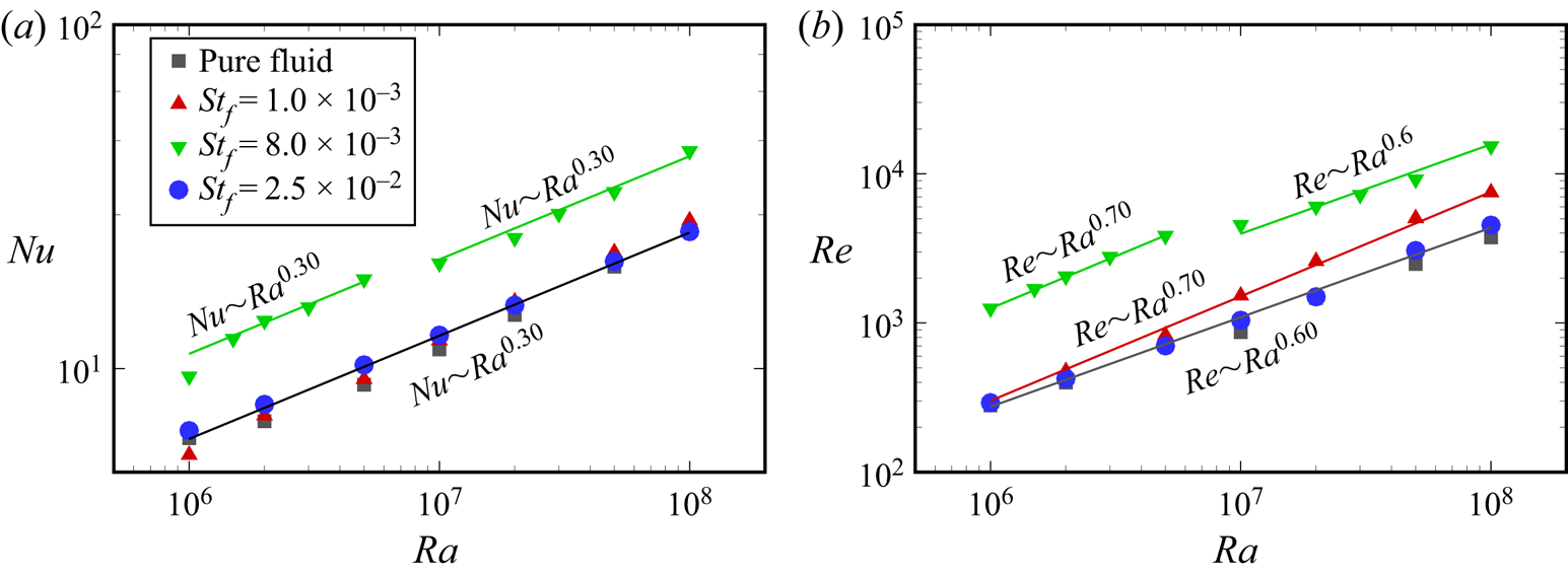
Figure 4(a,b) presents  $Nu$ and
 $Re$ as functions of
 $Ra$ for single-phase and the three Stokes numbers. We can see that for the small Stokes number (
 $St_f=1.0\times 10^{-3}$), both the
 $Nu$ and
 $Nu{\sim} Ra$ scaling are altered slightly, the scaling exponent is close to 0.3 which is the classic value for single-phase convection. However,
 $Re$ increases with increasing
 $Ra$ and the
 $Re{\sim} Ra$ scaling (with scaling exponent 0.7) is much steeper than that of single-phase case (with scaling exponent 0.6). This refers to the coupling effect of the particles and the fluid increases as
 $Ra$ increases, namely, the particle-induced kinetic energy is more important for larger
 $Ra$. For the large Stokes number (
 $St_f=2.5\times 10^{-2}$), particles go quickly through the flow field, there is no evident coupling between the distribution of particles and flow structures. Consequently, the feedback of particles is weak, so
 $Nu$ and
 $Re$ are altered slightly. This is in line with the observations in a cylindrical RB convection system by Oresta & Prosperetti (Reference Oresta and Prosperetti2013).
Log–log plot of  $Nu$ (a) and
 $Re$ (b) as functions of
 $Ra$ for the small, medium and large
 $St_f$.

For the medium Stokes number ( $St_f=8.0\times 10^{-3}$), both
 $Nu$ and
 $Re$ are significantly enhanced. The Rayleigh number is divided into two regimes. We can see that
 $Nu$ is increased by 90 % in regime
 $Ra<1.0\times 10^7$ and 60 % in regime
 $Ra>1.0\times 10^7$, whereas
 $Re$ is enhanced by up to 500 % for
 $Ra<1.0\times 10^7$ and 400 % for
 $Ra>1.0\times 10^7$. We notice that the exponent for
 $Nu{\sim} Ra$ scaling is 0.3 which is close to that for single-phase convection in both regimes. The exponent for
 $Re{\sim} Ra$ scaling is 0.7 in the low-
 $Ra$ regime and 0.6 in the high-
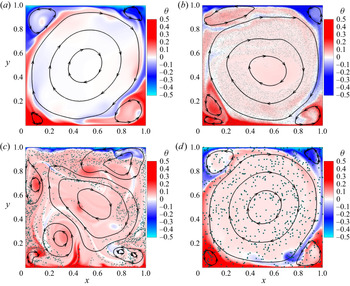
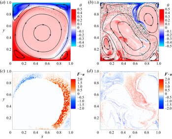
 $Ra$ regime. To reveal the discrepancies between these two regimes, we plot the flow fields in figure 5. In the low-
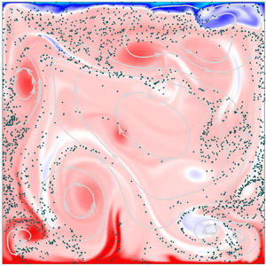
 $Ra$ regime shown in figure 5(a), it can be seen that preferential sweeping sends most of the particles into streaming zones of the LSC with a downward fluid; it makes these particles do positive work in the LSC. Nevertheless, in the high-
 $Ra$ regime shown in figure 5(b), preferential sweeping sends particles into streaming zones with both upward and downward fluid, but more particles are surrounded by downward fluid; overall the particles also do positive work but not that efficient as in the low-
 $Ra$ regime. Moreover, we further compare the work done by particles on the fluid as shown in figure 5(c,d), where
 $\boldsymbol {F}\boldsymbol {\cdot } \boldsymbol {u}$ represents the work done on the local fluid by the particles in unit time. It can be seen that not only is the region of positive work larger than the negative one, but also the positive work has a higher value for the low-
 $Ra$ regime. Consequently,
 $Nu$ and
 $Re$ are less enhanced in the high-
 $Ra$ regime. Another observation in the high-
 $Ra$ regime, from figure 5(b), is that the particles are apt to cluster near the edge of an eddy, and there are more particles near the downward part of the eddy, which can significantly speed up the eddy. As a result, the strength of turbulent momentum transfer and the structures of the thermal boundary layer are notably altered, which in turn enhances the heat transfer and flow intensity.
(a,b) Typical snapshots of the instantaneous temperature field (colour) and streamlines (black lines with arrows) for  $St_f=8.0\times 10^{-3}$ at
 $Pr=0.678$: (a)
 $Ra=10^6$ (low-
 $Ra$ regime); (b)
 $Ra=10^8$ (high-
 $Ra$ regime). Here 4 % of the total number of particles are shown for clarity. (c,d) The corresponding work done on the flow by the particles: (a)
 $Ra=10^6$ (low-
 $Ra$ regime); (b)
 $Ra=10^8$ (high-
 $Ra$ regime).

3.3. Energy dissipation in particle-laden RB convection
In the particle-laden RB system, the quantity of the particle-induced kinetic energy is important for the interphase coupling. The total kinetic energy of the fluid can be obtained from buoyancy and the interaction between particles and fluid, and is dissipated due to the effects of the fluid viscosity. So it is essential to quantify the contributions from buoyancy and fluid–particle interaction. One may use the exact relations of the energy dissipation rate in the system, in which the contribution of buoyancy and the effect of interaction can be separately investigated.
In turbulent single-phase RB convection, as a typical example for turbulent flows in a closed system, its local dissipation rates can be directly connected to the global heat transport through the convection cell via the two exact relations (Shraiman & Siggia Reference Shraiman and Siggia1990; Siggia Reference Siggia1994)
 \begin{equation} \langle\varepsilon_u\rangle=\frac{\nu^3}{H^4}Pr^{{-}2}Ra(Nu-1) \end{equation}
and
 \begin{equation} \langle\varepsilon_{\theta}\rangle=\kappa\frac{\varDelta^2}{H^2}Nu, \end{equation}
where  $\langle \cdot \rangle$ denotes an ensemble (or space–time) average. Based on these two relations, we can further derive the kinetic energy dissipation rate to study the budget balance of induced and dissipated kinetic energy in the particle-laden RB system. We use the subscript
 $d$ to denote dimensional physical quantities, and the dimensional Boussinesq equations are given as
 \begin{equation} {\partial}_{t,d}u_{i,d}+u_{j,d}{\partial}_{j,d}u_{i,d}={-}{\partial}_{i,d}p_d+\nu{\partial}_{j,d}^2u_{i,d}+\beta g\delta_{i3}\theta_d+f_{i,d}. \end{equation}
Multiply (3.4) by  $u_{i,d}$ to get
 \begin{equation} {\partial}_{t,d}\frac{\boldsymbol{u}_d^2}{2}={-}{\partial}_{j,d}\left(u_{i,d} \frac{\boldsymbol{u}_d^2}{2}\right)-u_{i,d}{\partial}_{i,d}p_d+\beta g\theta_du_{3,d}+ \nu u_{i,d}{\partial}_{j,d}^2u_{i,d}+f_{i,d}u_{i,d}. \end{equation}
Apply the product rule on the penultimate term of (3.5) to get
 \begin{equation} \nu u_{i,d}{\partial}_{j,d}^2u_{i,d}=\nu {\partial}_{j,d}(u_{i,d}{\partial}_{j,d}u_{i,d})-\nu {\partial}_{j,d}u_{i,d}{\partial}_{j,d}u_{i,d}. \end{equation}
Summarize terms which can be written as divergence, as follows:
 \begin{align} {\partial}_{t,d}\frac{\boldsymbol{u}_d^2}{2} &={-}{\partial}_{i,d}\left(u_{i,d}\frac{\boldsymbol{u}_d^2}{2}+u_{i,d}p_d+\nu \left({\partial} _{i,d}\frac{\boldsymbol{u}_d^2}{2}\right)\right) \nonumber\\ &\quad +\beta g\theta_du_{3,d}-\nu {\partial}_{j,d}u_{i,d}{\partial}_{j,d}u_{i,d}+f_{i,d}u_{i,d}. \end{align}
Apply stationarity (i.e. left-hand side equals zero) and volume average for (3.7); using Gauss’ theorem, the first term on the right-hand side vanishes as  $\boldsymbol {u}_d=0$ at all boundaries. Thus
 \begin{align} \langle\varepsilon_u\rangle &= \nu \langle{\partial}_{j,d}u_{i,d}{\partial}_{j,d}u_{i,d}\rangle=\beta g\langle \theta_du_{3,d}\rangle+\langle\, f_{i,d}u_{i,d}\rangle \nonumber\\ &= \beta g\frac{1}{H}\int^{H}_0 \textrm{d} z_d\langle \theta_du_{3,d}\rangle+\langle\, f_{i,d}u_{i,d}\rangle. \end{align}
Use the given definition of  $Nu$ to write
 \begin{equation} \langle \theta_du_{3,d}\rangle=\kappa\varDelta H^{{-}1}Nu+\kappa{\partial}_{3,d}\langle \theta_d\rangle, \end{equation}
using  $\langle \cdot \rangle _{A,t}$ to denote
 $z$-plane, time average and perform the integration over
 $z$ as follows:
 \begin{align} \langle\varepsilon_u\rangle &= \beta g\left(\kappa\varDelta H^{{-}1}Nu+ \frac{\kappa}{H}{\left[\langle \theta_d\rangle _{A,t}\right]}_0^L\right)+ \langle\, f_{i,d}u_{i,d}\rangle\nonumber\\ &= \beta g\left(\kappa\varDelta H^{{-}1}Nu+\frac{\kappa}{H}{\left(-\frac{\varDelta}{2}- \frac{\varDelta}{2}\right)}_0^L\right)+\langle\, f_{i,d}u_{i,d}\rangle\nonumber\\ &= \frac{\beta g\kappa\varDelta}{H}(Nu-1)+\langle\, f_{i,d}u_{i,d}\rangle\nonumber\\ &= \frac{\nu^3}{H^4}Pr^{{-}2}Ra(Nu-1)+\langle\, f_{i,d}u_{i,d}\rangle. \end{align}
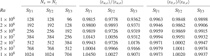
Equation (3.10) is the exact relation of kinetic energy dissipation rate for particle-laden RB convection. The two terms on the right-hand side are, respectively, the induced rate of kinetic energy of fluid due to thermal buoyancy and the correlation between momentum feedback and local fluid velocity. As for the thermal energy dissipation rate, it holds the same formulation as (3.3) for the single-phase fluid because the thermal feedback is not considered here. We can make use of the global exact relations, namely, (3.3) and (3.10) to verify the grid resolution of our simulations, according to Stevens, Verzicco & Lohse (Reference Stevens, Verzicco and Lohse2010). We compare the directly calculated dissipation rates (denoted with subscript  $c$) with those obtained from
 $Pr$,
 $Ra$,
 $Nu$ and the feedback term
 $\langle\, f_{i,d}u_{i,d}\rangle$ (denoted with subscript
 $e$) in table 3. It is seen from the table that the difference between the two results is small. That is to say the grid resolutions are fine enough to obtain accurate results, and the small structures can be well captured (Zhang et al. Reference Zhang, Zhou and Sun2017) and the feedback imposed by particles are properly calculated. It is also noted that, for the large
 $St_f$, the differences between the two kinetic energy dissipation rates are larger. We attribute this to the larger size of particles which not only affect the fluid cells contains the particles, but also affect the ambient fluid cells for a larger inertia of the particles.
The resolution in horizontal and vertical directions  $N_x$ and
 $N_z$,
 $\langle \varepsilon _{u,c}\rangle$ compared with that obtained from the exact relation
 ${\nu ^3}/{H^4}Pr^{-2}Ra(Nu-1)+\langle\, f_{i,d}u_{i,d}\rangle$ and
 $\langle \varepsilon _{\theta,c}\rangle$ compared with that obtained from the exact relation
 $\kappa {\varDelta ^2}/{H^2}Nu$ for different
 $Ra$ at small
 $St_{f1}=1.0\times 10^{-3}$, medium
 $St_{f2}=8.0\times 10^{-3}$ and large
 $St_{f3}=2.5\times 10^{-2}$.

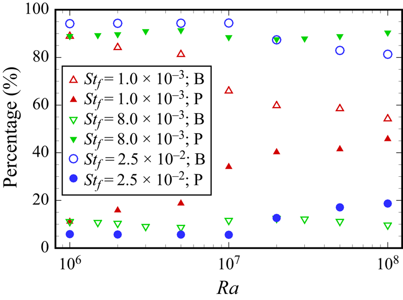
To develop deeper insights into the coupling effect, we note that the kinetic energies which are induced by thermal buoyancy and particles. We plot the variation of thermal buoyancy-induced kinetic energy and particle-induced kinetic energy with Rayleigh number for the three Stokes number cases in figure 6. For small  $St_f$, particle-induced kinetic energy is more and more important as
 $Ra$ increases, which further deduces larger alteration of the turbulent momentum transfer for larger
 $Ra$, resulting a higher
 $Re{\sim} Ra$ scaling exponent as shown in figure 4(b). It is indicated that particles are more apt to form clusters at larger
 $Ra$. For medium
 $St_f$, the particle-induced kinetic energy occupies 90 % of the total induced kinetic energy, so particles vastly accelerate the motion of the fluid, which can both affect the shape of the plumes and the thickness of the thermal boundary layer, so
 $Nu$ and
 $Re$ increase apparently as illustrated in figure 4. For large
 $St_f$, the particle-induced kinetic energy is less important, namely the coupling of particles and fluid is weak, so the flow structures as well as the heat transfer and the strength of turbulent momentum transfer are altered slightly as shown in figures 2 and 4.
The thermal buoyancy-induced energy and the particle-induced energy occupy the percentage of the total induced energy as the function of  $Ra$ for varying
 $St_f$ at B (buoyancy-induced kinetic energy) and P (particle-induced kinetic energy).

3.4. Settling and preferential concentration of particles
A knowledge of the average settling rate of small heavy particles in turbulent flows is important to many multiphase-flow problems involving particle transport and dispersion. The dynamic coupling between particles and fluid is germane to the settling and distribution of particles. In this section, we focus on the laws of settling and preferential concentration of different inertial particles.
3.4.1. Settling of particles
In still fluid, under the Stokesian particle assumption, the nominal terminal velocity of particles is  $v_{p,d}=\tau _{p}g$, where,
 $\tau _p=\rho _pd_p^2/(18\rho _R\nu )$ is the aerodynamic time constant of the particle. However, the settling of particles in turbulent flow could be quite different. There is no theoretical description of particles settling in a turbulent environment under two-way coupling. We are, therefore, motivated to give an estimation of the settling rate of particles in this complicated case.
On the one hand, we assume that the particles uniformly distribute along the height of the cell, so the averaged settling rate of particles, the percentage of the particles which pass the bottom plate in unit time of total number of particles in the fluid, is defined as
 \begin{align} S_{p,d}=\frac{{\displaystyle\sum_{t_d}^{t_d+dt_d}N_{p,bott}}/{dt_d}}{N_p}= \frac{{\vert\langle v_{p,d}\rangle_{N_{p,bott}}\vert\cdot dt_d\cdot\dfrac{N_p}{H}}/{dt_d}}{N_p}= \frac{\vert\langle v_{p,d}\rangle_{N_{p,bott}}\vert}{H}= \frac{\vert\langle v_{p}\rangle_{N_{p,bott}}\vert}{\sqrt{H/\beta g\varDelta}}. \end{align}
The non-dimensional averaged settling rate can be written as
 \begin{equation} S_{p}=\frac{S_{p,d}}{1/\sqrt{H/\beta g\varDelta}}=\vert\langle v_{p}\rangle_{N_{p,bott}}\vert, \end{equation}
where  $\sqrt {H/\beta g\varDelta }$ is the characteristic time scale which is the same as that used in (2.2)–(2.6),
 $N_{p,bott}$ is the number of particles which can pass across the bottom plate within a short time difference
 $dt_d$. Here
 $\langle \cdot \rangle _{N_{p,bott}}$ represents the sample
 $N_{p,bott}$ average of a specific physical parameter,
 $v_{p,d}$ is the particle velocity in the direction of gravity, specifically. Also, near the bottom plate,
 $v_{p,d}$ is negative, so we use the absolute value of
 $v_{p,d}$ in the above (3.11) and (3.12).
On the other hand, for the considered parameters, the gravity of the particle and the Stokes drag are dominant in the direction of gravity, so we can neglect the Saffman lift and thermophoresis, and we can obtain the following approximate relation in the direction of gravity according to (2.5):
 \begin{equation} \frac{\textrm{d} v_p}{\textrm{d} t}\simeq{-}\frac{1}{Fr_p^2}-\frac{C_D}{St_f}\left(v_p-v\right). \end{equation}
It is noticed that near the bottom wall, the particles are almost evenly settling, namely  ${\textrm {d} v_p}/{\textrm {d} t}=0$, and the fluid velocity in the direction of gravity is very small, namely
 $v\simeq 0$. Besides, on account of that Stokes numbers are sufficiently small, so particles quickly response the ambient flow in the horizontal direction, namely
 $u_p-u\simeq 0$, so we can get
 \begin{equation} \vert\langle v_{p}\rangle_{N_{p,bott}}\vert\simeq\frac{St_f}{Fr_p^2}\cdot \frac{1}{1+0.15\left({Pr}/{Ra}\right)^{0.678/2}\cdot\left({d_p}/{H}\vert v_p-v\vert\right)^{0.678}}. \end{equation}
By ignoring  $0.15({Pr}/{Ra})^{0.678/2}({d_p}/{H}\vert v_p-v\vert )^{0.678}$ which is small relative to unity in the present parameters. So we can obtain the approximate relation
 \begin{equation} S_{p}\simeq\frac{1}{18}\frac{1}{Fr_p^2}\frac{\rho_p}{\rho_R}\cdot \frac{d_p^2}{H^2}\cdot\sqrt{\frac{Ra}{Pr}}. \end{equation}
On account of the approximate assumption and the simplification in the derivative procedure, there are three causes that can result in a small adjustment for (3.15):
(1) the distribution of particles is not uniform along with the height of the cell;
(2) the effect of Saffman lift and thermophoresis may not be neglected near the bottom wall;
(3) the value of
$0.15({Pr}/{Ra})^{0.678/2}({d_p}/{H}\vert v_p-v\vert )^{0.678}$ may be large for specific parameters.

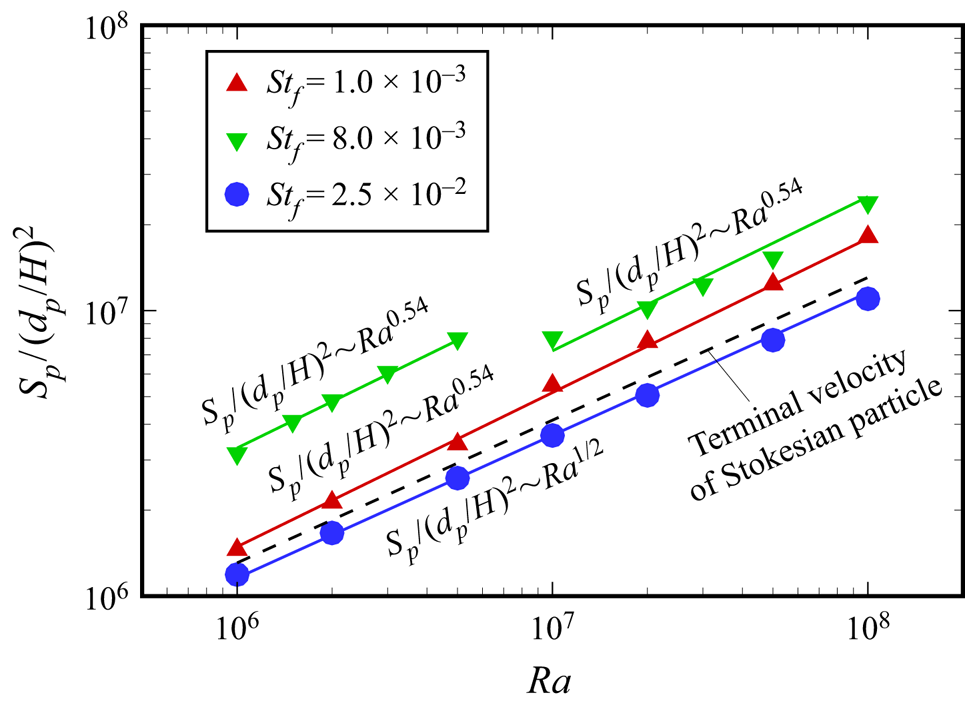
Figure 7 shows the ratio of the non-dimensional averaged settling rate of particles to the square of non-dimensional particle diameters as a function of  $Ra$ for small, medium and large
 $St_f$. We can see that for all the three cases, the data can be well-described by a power-law relation
 $S_p/(d_p/H)^2{\sim} Ra^{1/2}$ which, remarkably, agrees with our theoretical prediction in (3.15). The scaling exponents slightly deviate from 0.5 due to the assumptions we made.
The ratio of the averaged settling rate of particles with the non-dimensional particle diameters as a function of  $Ra$ for small, medium and large
 $St_f$.

For small  $St_f=1\times 10^{-3}$, the averaged settling rate of particles is slightly larger than the nominal terminal velocity, such an increase is owing to the contribution of the LSC. This is consistent with the findings in the homogeneous isotropic turbulence (Tom & Bragg Reference Tom and Bragg2019). For large
 $St_f=2.5\times 10^{-2}$, the averaged particle settling rate is slightly smaller than the nominal terminal velocity of particles, which is due to the uniform distribution of particles and the upward flow impedes settling. This is in line with the observations in particle-laden grid generated turbulence (Nielsen Reference Nielsen1993; Good, Gerashchenko & Warhaft Reference Good, Gerashchenko and Warhaft2012).
For medium  $St_f=8\times 10^{-3}$, the regime of the averaged particles settling rate is subdivided into low- and high-
 $Ra$ number regimes. For both low- and high-
 $Ra$ number regimes, the averaged particle settling rate is obviously larger than the nominal terminal velocity, which is related to the fact that the inertial bias is coupled to a preferential sweeping of the particles in downward fluid motions (Maxey Reference Maxey1987; Wang & Maxey Reference Wang and Maxey1993) and the combined effect of inertia and preferential sweeping may send particles into streaming zones with downward fluid velocity, see in figure 5. Moreover, a recent study (Tom & Bragg Reference Tom and Bragg2019) shows that even for quite small Stokes numbers, a relatively large flow scale contributes to the settling of the particles. This refers to the fact that the enhanced LSC further increases the settling of the particles. As particles tend to settle in the downward-flow side of a cell (Maxey & Corrsin Reference Maxey and Corrsin1986; Bosse, Kleiser & Meiburg Reference Bosse, Kleiser and Meiburg2006) that leads to a larger settling rate than the terminal velocity. Note that in the low-
 $Ra$ regime, the combined effect of inertia and the preferential sweeping sends particles into streaming zones with the downward fluid velocity as shown in figure 5(a), where the strength of LSC is not strong enough to carry the inertial particles upwards. For the high-
 $Ra$ regime, the LSC can carry the inertial particles upwards, preferential sweeping is also relevant to the edges of the eddy and rotational zones. Also, under the effect of Stokes drag, the motion of particles is slowed down near the upwards fluid, consequently, the averaged settling rate of particles increases more for the low-
 $Ra$ regime.
3.4.2. Preferential concentration of particles
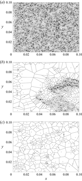
As for the preferential concentration of particles, it can be identified through Voronoï diagrams (Monchaux et al. Reference Monchaux, Bourgoin and Cartellier2010; Park et al. Reference Park, O'Keefe and Richter2018). The area  $A$ of a Voronoï cell is the inverse of the local concentration of particles, therefore, the investigation of Voronoï cell field is strictly equivalent to that of a local concentration field. Figure 8 presents the typical snapshots of the distribution of particles as well as their Voronoï diagram. It is seen from figure 8 that the distribution of areas of Voronoï cell is such as that of a random Poisson process (RPP) for small and large
 $St_f$ and is more concentrated at small cells for medium
 $St_f$. This indicates that particles uniformly distribute in the flow field for small and large
 $St_f$, and are locally concentrated for medium
 $St_f$.
Typical snapshots of the distribution of particles and its Voronoï diagram for  $Ra=10^8$ at
 $Pr=0.678$: (a)
 $St_f=1.0\times 10^{-3}$; (b)
 $St_f=8.0\times 10^{-3}$; (c)
 $St_f=2.5\times 10^{-2}$. For clarity, we show only bottom left-hand corner of the computational domain.

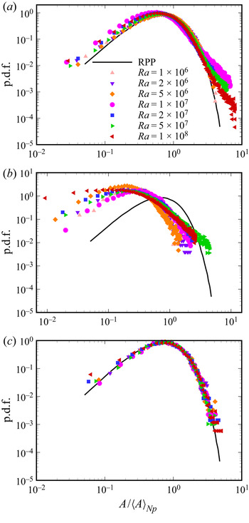
We now come to the statistics of the Voronoï cells. Figure 9 shows the probability density functions (p.d.f.s) of Voronoï cells obtained at small, medium and large  $St_f$, all data have been normalized with their averaged Voronoï area
 ${\langle A\rangle }_{N_p}$. In the figures, it is noteworthy that the p.d.f. of RPP fits well with these data for small and large
 $St_f$, it indicates that the distribution of particles is rather random. However, for medium
 $St_f$, the p.d.f.s of small Voronoï areas are above the RPP while we observe the opposite for larger Voronoï areas; this is consistent with the intuitive image of preferential concentration.
The p.d.f.s of normalized Voronoï area  $A/{{\langle A \rangle }_{N_p}}$ for
 $10^6\le Ra\le 10^8$ at
 $Pr=0.678$: (a)
 $St_f=1.0\times 10^{-3}$; (b)
 $St_f=8.0\times 10^{-3}$; (c)
 $St_f=2.5\times 10^{-2}$ (each p.d.f. is calculated from one typical snapshot).

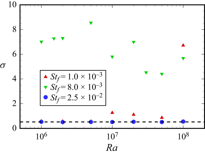
The above results qualitatively show the preferential concentration, to further quantitatively describe the distribution of particles. The standard deviations of Voronoï areas are depicted in figure 10 where the dashed line denotes the standard deviation of RPP that is equal to 0.53. Momenifar & Bragg (Reference Momenifar and Bragg2020) recently showed that the standard deviation of Voronoï areas is dominated by the void regions of the flow rather than the clustered regions. So we here concentrate on the global distribution of particles rather than the cluster regions. We can see that for the small Stokes number ( $St_f=1.0\times 10^{-3}$), the standard deviations of Voronoï areas are approaching 0.53 for
 $Ra<10^7$, and they significantly exceed 0.53 for
 $Ra\ge 10^7$. This reveals the existence of high and low concentration events compared with the RPP case for
 $Ra\ge 10^7$. As for the medium Stokes number (
 $St_f=8.0\times 10^{-3}$), all the standard deviations of Voronoï areas significantly exceeds 0.53; this refers to the fact that there are many high and low concentration events, namely preferential clusters, compared with the RPP. Also, for the large Stokes number (
 $St_f=2.5\times 10^{-2}$), all the standard deviations of Voronoï areas are approach 0.53, namely, the distributions of particles are more like RPP.
Standard deviations  $\sigma$ of the Voronoï areas as a function of
 $Ra$ at
 $Pr=0.678$ for
 $St_f=1.0\times 10^{-3}$,
 $St_f=8.0\times 10^{-3}$ and
 $St_f=2.5\times 10^{-2}$.

In addition, the radial distribution functions (RDFs) are also an effective measure for the study of particle clustering, and its distinct advantages over the Voronoï diagrams is not biased by the number of particles simulated (Ireland, Bragg & Collins Reference Ireland, Bragg and Collins2016). The RDF  $g(r)$ is defined as the ratio of the number of particle pairs at a given separation
 $r$ to the expected number of particle pairs in a uniformly distributed particle field,
 \begin{equation} g(r)=\frac{N_i/V_i}{N/V}. \end{equation}
Here,  $N_i$ is the number of particle pairs that lie within a ring with an average radius
 $r$ and a radial width
 $\Delta r$,
 $V_i$ is the area of the ring and
 $N$ is the total number of particle pairs located in the local area
 $V$. An RDF in excess of unity indicates a clustered particle field. When the distribution of RDF is in the vicinity of one, it corresponds to uniformly distributed particles. Figure 11 presents the RDFs at small, medium and large
 $St_f$. In the figure, it is noteworthy that, in agreement with the observation in Voronoï diagram, the distribution of particles is rather uniform for small and large
 $St_f$. While it can be noted that particles exhibit clustering at small scale, this is the nature of RPP. What is more, for small
 $St_f$, the larger
 $Ra$ is the more significant trend and particle exhibit clustering. As for the medium
 $St_f$, we see that particle clustering peaks at all
 $Ra$ shown. Moreover, in contrast to small
 $St_f$, the smaller
 $Ra$ is, the stronger the degree of clustering is, and this can be further deduced from the distribution of particles as shown in figure 5.
The RDFs at three different values of  $Ra$ for
 $St_{f1}=1.0\times 10^{-3}$,
 $St_{f2}=8.0\times 10^{-3}$ and
 $St_{f3}=2.5\times 10^{-2}$, plotted as a function of the non-dimensional separation
 $r$. Here
 $r$ is non-dimensionalized by the characteristic length
 $H$.

In summary, in the particle-laden RB convection, the particle-induced kinetic energy directly correlates with the two-phase coupling, and has a significant effect on the heat transfer, the strength of turbulent momentum transfer as well as the settling and preferential concentration of particles. It is found that at small and large Stokes numbers, the particle-induced kinetic energy is less important, so the heat transfer is changed a little, however, at medium Stokes number, the particle-induced kinetic energy becomes dominating, which induces a great enhancement of heat transfer.
4. Conclusion
We carried out the direct numerical simulations combined with the Lagrangian point-particle mode for the RB convection laden with isothermal inertial particles in the range of  $1\times 10^6\le Ra\le 1\times 10^8$ at
 $Pr=0.678$ for three Stokes numbers
 $St_f=1\times 10^{-3}$,
 $St_f=8\times 10^{-3}$ and
 $St_f=2.5\times 10^{-2}$. We also derived the exact relation for the kinetic energy dissipation in particle-laden RB convection, which refers to the budget balance of induced and dissipated kinetic energy. The correlation between momentum feedback and local fluid velocity is quantified from the particle-induced kinetic energy. Moreover, we derived the power-law relation of the averaged particles settling rate versus the Rayleigh number, i.e.
 $S_p/(d_p/H)^2{\sim} Ra^{1/2}$, and validated it by using our data.
We found for the small Stokes number  $St_f=1\times 10^{-3}$ case, the feedback of particles is more significant at large
 $Ra$, namely, the particle-induced kinetic energy becomes larger in the large
 $Ra$ regime; consequently,
 $Re$ exhibits a much steeper scaling with
 $Ra$ than the single-phase flow. The averaged settling rate of particles is larger than the nominal terminal velocity of Stokesian particles and exhibits a much steeper scaling with
 $Ra$ than the nominal terminal velocity. Besides, the distribution of particles is more concentrated as
 $Ra$ increases.
As for the medium Stokes number  $St_f=8\times 10^{-3}$, the clusters caused by the preferential sweeping of particles is relevant to the edges of eddies and rotational zones, which makes particles effectively do work on these eddies and even change the boundary layer. Consequently, the
 $Re$ and
 $Nu$ are significantly increased, the total induced kinetic energy is dominated by particle-induced kinetic energy, and the averaged particle settling rate is significantly larger than the terminal velocity of Stokesian particles. What is more, there are two regimes, namely low- and high-
 $Ra$ number regimes, for this Stokes number. In the low-
 $Ra$ number regime, preferential sweeping only sends particles into the downward fluid of LSC, so almost all particles do positive work on the LSC. Nevertheless, in the high-
 $Ra$ regime, preferential sweeping sends particles into streaming zones with both upward and downward fluid, but more particles are surrounded by downward fluid; overall the particles also do positive work but not that efficient as in the low-
 $Ra$ regime. As a result, the
 $Re$ and
 $Nu$ are increased to a greater extent than that in high-
 $Ra$ number regime.
Finally, for the large Stokes number  $St_f=2.5\times 10^{-2}$, particles go quickly through the flow field as a result of their heavy weight. Consequently, the flow structures as well as the global features of flow field are altered little. Besides, the motion of upwards fluid will slow down the settling of particles, so the averaged settling rate of particles is slower than the terminal velocity of Stokesian particles.
Acknowledgments
The authors appreciate the valuable suggestions of the reviewer. We are also thankful to J. Shen for his useful discussion in the implementation of the RDF.
Funding
This work was supported by the Natural Science Foundation of China (grant nos. 91852111, 12172207, 92052201, 11825204 and 11972220), Science and Technology Innovation Plan Of Shanghai Science and Technology Commission (STCSM) under project no. 19JC1412802.
Declaration of interests
The authors report no conflict of interest.