1. Introduction
A detailed near-tip analysis of a planar hydraulic fracture shows (Peirce & Detournay Reference Peirce and Detournay2008) that the governing equations reduce to those of a steadily propagating semi-infinite hydraulic fracture under conditions of elastic plane strain. It is therefore important to analyse the problem of a semi-infinite hydraulic fracture, as it governs the behaviour of the tip region of arbitrarily shaped finite hydraulic fractures and influences their global behaviour. Recognizing the necessity of accurate fracture tip modelling, the hydraulic fracturing methodology known as the implicit level set algorithm (ILSA) (Peirce & Detournay Reference Peirce and Detournay2008) was developed to embed the solution of the appropriate semi-infinite hydraulic fracture into every fracture tip element. This procedure is shown to produce accurate results even on a relatively coarse mesh (Lecampion et al. Reference Lecampion, Peirce, Detournay, Zhang, Chen, Bunger, Detournay, Napier, Abbas, Garagash, Cundall, Bunger, McLennan and Jeffrey2013). This technique has also been used in the context of the extended finite element method to model the propagation of hydraulic fractures (Gordeliy & Peirce Reference Gordeliy and Peirce2013). It is therefore important to develop a fast and accurate solution methodology to solve the semi-infinite fracture problem so that it can be used to increase the performance of various hydraulic fracturing simulators in this multiscale environment.
To analyse the problem of a propagating semi-infinite hydraulic fracture, we adopt a mathematical model that assumes that (i) the fracturing fluid is Newtonian, (ii) the fluid front coincides with the fracture tip (i.e. there is no fluid lag), (iii) the material is brittle and is linear elastic, and (iv) the leak-off is modelled by a one-dimensional diffusion process via Carter’s model, which is applicable when the diffusion length scale is much smaller than the fracture length (Carter Reference Carter, Howard and Fast1957). Other studies that involve a steadily propagating semi-infinite hydraulic fracture consider the effects of power-law fluid (Desroches et al. Reference Desroches, Detournay, Lenoach, Papanastasiou, Pearson, Thiercelin and Cheng1994; Lenoach Reference Lenoach1995), account for the fluid lag (Garagash & Detournay Reference Garagash and Detournay2000) or include poroelastic effects (Kovalyshen & Detournay Reference Kovalyshen2013). However, most of these studies focus on some limiting regimes of propagation (Detournay Reference Detournay2004). The first problem we consider has already been addressed in Garagash, Detournay & Adachi (Reference Garagash, Detournay and Adachi2011), where a special numerical scheme with built-in asymptotic solutions was used. Unfortunately, due to the complexity of that numerical approach, it is not possible to obtain a rapid solution for the purpose of embedding it into a hydraulic fracturing simulator that exploits the tip asymptotics such as the ILSA strategy (Peirce & Detournay Reference Peirce and Detournay2008). A partial solution was obtained (Peirce Reference Peirce2015) in which the pre-computed semi-infinite fracture toughness-to-viscous solution was interpolated to capture the multiscale fracture tip behaviour in the hydraulic fracturing simulator ILSA. In this case the tip solution without leak-off was utilized, so that one-dimensional interpolation could be used to provide satisfactory precision, albeit at a noticeably increased computational cost. A similar interpolation-based scheme for the tip solution with leak-off does not seem feasible since two-dimensional interpolation is required. This would substantially complicate the algorithm, might introduce significant numerical errors and would dramatically degrade the overall computational performance of the hydraulic fracture simulator.
To address this problem, following Garagash et al. (Reference Garagash, Detournay and Adachi2011), this study first outlines the equations that govern the problem of a semi-infinite hydraulic fracture with leak-off in § 2.1. Then, § 2.2 reformulates the original governing integro-differential equations with a singular kernel used in Garagash et al. (Reference Garagash, Detournay and Adachi2011) in the form of a single integral equation with a non-singular kernel. This allows us to use standard numerical techniques to obtain the multiscale solution rapidly. In § 2.3 we use this new formulation to approximate the problem by a separable ordinary differential equation whose closed-form solution captures the multiscale behaviour with sufficient accuracy and simplicity that it can be readily used to model the tip behaviour in hydraulic fracture simulators such as ILSA (Peirce & Detournay Reference Peirce and Detournay2008). Applications of the proposed formulation are not limited to the class of multiscale semi-infinite hydraulic fracture problems described above but include other similar problems. To demonstrate this, § 3 considers the problem of a buoyancy-driven plane strain hydraulic fracture (see, e.g. Spence & Turcotte Reference Spence and Turcotte1985, Lister Reference Lister1990, Roper & Lister Reference Roper and Lister2007) by rewriting the governing equations in terms of a single integral equation with a non-singular kernel.
2. A semi-infinite hydraulic fracture with leak-off
2.1. Problem formulation and regimes of propagation
We consider the problem of a one-dimensional semi-infinite hydraulic fracture propagating with a velocity
 $V$
under plane strain elastic conditions (Garagash et al.
Reference Garagash, Detournay and Adachi2011). To deal with this problem, it is convenient to introduce a moving coordinate system, in which the fracture tip is always located at the origin and the
 $x$
denotes the distance from a point inside the fracture to the tip. As follows from Peirce & Detournay (Reference Peirce and Detournay2008) and Garagash et al. (Reference Garagash, Detournay and Adachi2011), the lubrication equation that describes the fluid flow along the fracture can be written as
 $$\begin{eqnarray}{\displaystyle \frac{w^{2}}{{\it\mu}^{\prime }}}\,{\displaystyle \frac{\text{d}p}{\text{d}x}}=V+2C^{\prime }V^{1/2}{\displaystyle \frac{x^{1/2}}{w}},\end{eqnarray}$$
where
 $w$
is the fracture width,
 $p$
is the fluid pressure,
 $V$
is the fracture propagation velocity, while
 ${\it\mu}^{\prime }=12{\it\mu}$
is the scaled fluid viscosity and
 $C^{\prime }=2C_{L}$
is the scaled Carter leak-off coefficient. We note a typographical error in Garagash et al. (Reference Garagash, Detournay and Adachi2011), in which the factor of two is missing in front of the leak-off term in (2.1), which propagates into the remaining results. Assuming that the rock is a linear elastic medium, the equilibrium of the rock surrounding the fracture can be expressed as the following integral equation which relates the fluid pressure to the fracture width:
 $$\begin{eqnarray}p(x)={\displaystyle \frac{E^{\prime }}{4{\rm\pi}}}\int _{0}^{\infty }\,{\displaystyle \frac{\text{d}w(s)}{\text{d}s}}\,{\displaystyle \frac{\text{d}s}{x-s}},\end{eqnarray}$$
where
 $E^{\prime }=E/(1-{\it\nu}^{2})$
is the plane strain elastic modulus. The latter equation can be inverted (Garagash & Detournay Reference Garagash and Detournay2000) to obtain
 $$\begin{eqnarray}w={\displaystyle \frac{K^{\prime }}{E^{\prime }}}x^{1/2}+{\displaystyle \frac{4}{{\rm\pi}E^{\prime }}}\int _{0}^{\infty }K(x,s)p(s)\,\text{d}s,\end{eqnarray}$$
where
 $K^{\prime }=\sqrt{32/{\rm\pi}}K_{Ic}$
,
 $K_{Ic}$
denotes the fracture toughness and the kernel is given by
 $$\begin{eqnarray}\displaystyle K(x,s)=\ln \left|{\displaystyle \frac{x^{1/2}+s^{1/2}}{x^{1/2}-s^{1/2}}}\right|-2{\displaystyle \frac{x^{1/2}}{s^{1/2}}}. & & \displaystyle\end{eqnarray}$$
To close the system (2.1) and (2.3), one needs to include a fracture propagation criterion, which states that
 $$\begin{eqnarray}w={\displaystyle \frac{K^{\prime }}{E^{\prime }}}x^{1/2},\quad x\rightarrow 0.\end{eqnarray}$$
As can be seen from (2.5), the fracture width vanishes at the fracture tip. This implies that the pressure gradient in (2.1) should be infinite at the tip to ensure that the fracture velocity is finite. This feature makes the system (2.1), (2.3) and (2.5) challenging to solve numerically.
An asymptotic analysis of (2.1), (2.3) and (2.5) shows that there are three limiting regimes of propagation, namely toughness (denoted by
 $k$
), leak-off (denoted by
 $\tilde{m}$
) and viscous (denoted by
 $m$
) (see, e.g. Garagash et al.
Reference Garagash, Detournay and Adachi2011). The toughness regime corresponds to the situation in which the effects of fluid viscosity and leak-off can be neglected. The leak-off propagation regime occurs in situations when both the fracture toughness is small and the fluid flow inside the fracture is primarily balanced by the flux due to the fluid leaking into the surrounding rock. The viscous propagation regime corresponds to the situation in which both the fracture toughness and the leak-off are negligible. These asymptotic (vertex) solutions are respectively given by
 $$\begin{eqnarray}w_{k}={\displaystyle \frac{K^{\prime }}{E^{\prime }}}x^{1/2},\quad w_{\tilde{m}}={\it\beta}_{\tilde{m}}\left({\displaystyle \frac{4{\it\mu}^{\prime 2}VC^{\prime 2}}{E^{\prime 2}}}\right)^{1/8}x^{5/8},\quad w_{m}={\it\beta}_{m}\left({\displaystyle \frac{{\it\mu}^{\prime }V}{E^{\prime }}}\right)^{1/3}x^{2/3},\end{eqnarray}$$
where
 ${\it\beta}_{\tilde{m}}=4/(15^{1/4}(\sqrt{2}-1)^{1/4})$
and
 ${\it\beta}_{m}=2^{1/3}3^{5/6}$
.
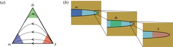
(a) The parametric triangle (after Garagash et al.
Reference Garagash, Detournay and Adachi2011), which indicates three regimes of propagation: the toughness regime (
 $k$
vertex), the leak-off regime (
 $\tilde{m}$
vertex) and the viscous regime (
 $m$
vertex). Lines inside the triangle show possible trajectories (assuming a spatial coordinate increasing away from the tip) in parametric space. (b) The schematics of a fracture and the regions where the asymptotic solutions apply.

Knowledge of only the vertex solutions is not sufficient, since hydraulic fractures are known to transition from one vertex to another (Detournay Reference Detournay2004). With regard to the semi-infinite hydraulic fracture problem under consideration, these regimes occur at different length scales within the fracture, see figure 1. The toughness regime is present near the fracture tip, and, as one moves further from the tip (if the leak-off is significant), the leak-off regime appears, followed by the viscous regime at infinity. The transition is often schematically illustrated as a path inside a parametric triangle (Garagash et al.
Reference Garagash, Detournay and Adachi2011), see figure 1. Vertices represent single-process limiting solutions (2.6), while lines with arrows indicate possible transition paths from the
 $k$
vertex (near the tip) to the
 $m$
vertex (far-field behaviour). It should be noted that without leak-off the transition occurs solely along the
 $mk$
edge, while in the case of large leak-off the transition occurs along the
 $\tilde{m}k$
and
 $m\tilde{m}$
edges. The coloured zones inside the triangle indicate the regions of applicability of the vertex solutions. To determine the solution in the transition regimes (the inner white area of the parametric triangle), one has to solve (2.1), (2.3) and (2.5) numerically. The numerical analysis of this problem has proven to be very challenging due to the multiple length scales involved and the singular behaviour of the fluid pressure at the tip. This study introduces an alternative approach, which allows us to avoid solving a singular problem and enables us to find the fracture geometry at all length scales in a numerically efficient way.
2.2. Alternative problem formulation and numerical solution
One of the biggest obstacles to solving the system of (2.1), (2.3) and (2.5) numerically lies in an accurate evaluation of the flux in (2.1), given that the fluid pressure is singular at the fracture tip. To mitigate the problem, this section aims to rewrite the system of equations in a form in which the fluid pressure does not enter the problem. We first note that the elasticity equation (2.3) can be integrated by parts to yield
 $$\begin{eqnarray}w={\displaystyle \frac{K^{\prime }}{E^{\prime }}}x^{1/2}-{\displaystyle \frac{4}{{\rm\pi}E^{\prime }}}\int _{0}^{\infty }F(x,s)\,{\displaystyle \frac{\text{d}p}{\text{d}s}}\,\text{d}s,\end{eqnarray}$$
where
 $$\begin{eqnarray}K(x,s)={\displaystyle \frac{\partial F(x,s)}{\partial s}},\quad F(x,s)=(s-x)\ln \left|{\displaystyle \frac{x^{1/2}+s^{1/2}}{x^{1/2}-s^{1/2}}}\right|-2x^{1/2}s^{1/2}.\end{eqnarray}$$
It should be noted here that
 $$\begin{eqnarray}\displaystyle \lim _{s\rightarrow \infty }F(x,s)p(s)=4x\lim _{s\rightarrow \infty }p(s)=0,\quad \lim _{s\rightarrow 0}F(x,s)p(s)=-4x^{1/2}\lim _{s\rightarrow 0}s^{1/2}p(s)=0, & & \displaystyle \nonumber\\ \displaystyle & & \displaystyle\end{eqnarray}$$
since for the viscous far-field solution
 $p(s)\propto s^{-1/3}$
as
 $s\rightarrow \infty$
and for the toughness near-tip solution
 $p(s)\propto \ln (s)$
as
 $s\rightarrow 0$
, see, e.g. Garagash et al. (Reference Garagash, Detournay and Adachi2011). Then, the pressure gradient can be substituted into (2.7) from the lubrication equation (2.1) to find
 $$\begin{eqnarray}w(x)={\displaystyle \frac{K^{\prime }}{E^{\prime }}}x^{1/2}-{\displaystyle \frac{4}{{\rm\pi}E^{\prime }}}\int _{0}^{\infty }F(x,s){\displaystyle \frac{{\it\mu}^{\prime }}{w(s)^{2}}}\left[V+2C^{\prime }V^{1/2}{\displaystyle \frac{s^{1/2}}{w(s)}}\right]\,\text{d}s.\end{eqnarray}$$
Equation (2.10) is an integral equation for
 $w(x)$
only, which already simplifies the original problem since the pressure, which is singular at the tip, is not a part of the solution. It should be noted that a similar integration by parts was also performed in Spence, Sharp & Turcotte (Reference Spence, Sharp and Turcotte1987) and Lister (Reference Lister1990). Moreover, an equation similar to (2.10) was formulated in Spence et al. (Reference Spence, Sharp and Turcotte1987), but it was only used for the asymptotic analysis. By introducing the scaled quantities
 $$\begin{eqnarray}\tilde{w}={\displaystyle \frac{E^{\prime }w}{K^{\prime }x^{1/2}}},\quad {\it\chi}={\displaystyle \frac{2C^{\prime }E^{\prime }}{V^{1/2}K^{\prime }}},\quad \tilde{x}=(x/l)^{1/2},\quad \tilde{s}=(s/l)^{1/2},\quad l=\left({\displaystyle \frac{K^{\prime 3}}{{\it\mu}^{\prime }E^{\prime 2}V}}\right)^{2},\end{eqnarray}$$
equation (2.10) can be further reduced to
 $$\begin{eqnarray}\tilde{w}(\tilde{x})=1+{\displaystyle \frac{8}{{\rm\pi}}}\int _{0}^{\infty }G(\tilde{s}/\tilde{x})\left[{\displaystyle \frac{1}{\tilde{w}(\tilde{s})^{2}}}+{\displaystyle \frac{{\it\chi}}{\tilde{w}(\tilde{s})^{3}}}\right]\text{d}\tilde{s},\end{eqnarray}$$
where
 $l$
is the length scale, the dimensionless parameter
 ${\it\chi}$
characterizes the leak-off and the kernel is
 $$\begin{eqnarray}G(t)={\displaystyle \frac{1-t^{2}}{t}}\ln \left|{\displaystyle \frac{1+t}{1-t}}\right|+2.\end{eqnarray}$$
It should be noted that a similar length scale
 $l$
is used in Garagash et al. (Reference Garagash, Detournay and Adachi2011) to describe the transition regime along the
 $mk$
edge (denoted by
 $l_{mk}$
there). In this scaling, the propagation condition (2.5) reduces to
 $$\begin{eqnarray}\tilde{w}(0)=1.\end{eqnarray}$$
Given the fact that the kernel
 $G(t)$
is positive and not singular (
 $G(0)=4$
,
 $G(t)\approx 4/(3t^{2})$
for
 $t\gg 1$
), and that
 $\tilde{w}\geqslant 1$
, the integral equation (2.12) is amenable to direct numerical solution, without introducing any asymptotic behaviour into the solution.
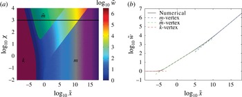
(a) Variation of the scaled fracture opening
 $\tilde{w}$
versus the scaled distance
 $\tilde{x}$
and leak-off parameter
 ${\it\chi}$
. The red, green and blue areas indicate the regions of applicability of the toughness, leak-off and viscous vertex solutions (2.15). The black line indicates the solution that corresponds to
 ${\it\chi}=10^{3}$
. (b) Numerical solution for
 ${\it\chi}=10^{3}$
versus
 $\tilde{x}$
(black line) and vertex asymptotic solutions
 $m$
(viscous, blue line),
 $\tilde{m}$
(leak-off, green line) and
 $k$
(toughness, red line).

It is instructive to check whether the vertex solutions can be deduced directly from (2.12). The first term on the right-hand side of (2.12) represents the effect of fracture toughness, the second term (the first term under the integral sign) represents the effect of the fluid viscosity and the third term represents the effect of leak-off. By substituting
 $\tilde{w}=C\tilde{x}^{{\it\alpha}}$
into (2.12) and keeping only one term that corresponds to either toughness, viscosity or leak-off, we obtain
 $$\begin{eqnarray}\tilde{w}_{k}=1,\quad \tilde{w}_{\tilde{m}}={\it\beta}_{\tilde{m}}{\it\chi}^{1/4}\tilde{x}^{1/4},\quad \tilde{w}_{m}={\it\beta}_{m}\tilde{x}^{1/3},\end{eqnarray}$$
which correspond exactly to the asymptotic solutions (2.15) in the scaled coordinates. It should be noted here that the values of
 ${\it\beta}_{m}$
and
 ${\it\beta}_{\tilde{m}}$
are calculated based on the fact that
 $$\begin{eqnarray}\int _{0}^{\infty }{\displaystyle \frac{G(t)}{t^{{\it\alpha}}}}\,\text{d}t={\displaystyle \frac{2{\rm\pi}}{{\it\alpha}(2-{\it\alpha})}}\tan \left({\displaystyle \frac{{\rm\pi}}{2}}{\it\alpha}\right),\end{eqnarray}$$
where
 $-1<{\it\alpha}<1$
(the integral does not converge for values of
 ${\it\alpha}$
that are outside this interval).
In order to solve (2.12) numerically, the integral is discretized using Simpson’s rule, and the resultant system of nonlinear algebraic equations is solved using Newton’s method. To capture all the length scales present in the solution, grid points are distributed uniformly on a logarithmic scale. To mitigate the error caused by a finite upper limit of the integral in (2.12), the fracture opening solution that corresponds to the last several grid points (on the logarithmic scale) is discarded. Figure 2(a) shows the variation of the solution,
 $\tilde{w}$
, versus
 ${\it\chi}$
and
 $\tilde{x}$
. To indicate the regions of applicability of the vertex solutions (2.15), these solutions are shifted upwards by
 $10^{-2}$
on a log scale (to highlight regions where the relative difference between the numerical and asymptotic solutions is smaller than 2.3 %) and then superimposed on the numerical solution. It should be noted that this map of the regimes is very similar to the schematics in Garagash et al. (Reference Garagash, Detournay and Adachi2011). Figure 2(b) shows the variation of the scaled fracture opening versus
 $\tilde{x}$
for
 ${\it\chi}=10^{3}$
, which corresponds to the black line shown in figure 2(a). The vertex asymptotic solutions are superimposed. One can observe a transition from the toughness-dominated regime, to the leak-off and, finally, to the viscous-dominated regime. This transition is consistent with the schematics shown in figure 1.
2.3. Approximate analytical solution
Numerical solution of (2.12) provides an accurate way of solving the problem under consideration. For some practical applications, e.g. for implementing this solution in a hydraulic fracturing simulator such as ILSA (Peirce & Detournay Reference Peirce and Detournay2008), it is desirable to obtain an easily evaluated approximate solution that is reasonably accurate. To derive such an approximate solution, one can differentiate (2.12) to obtain
 $$\begin{eqnarray}{\displaystyle \frac{\text{d}\tilde{w}(\tilde{x})}{\text{d}\tilde{x}}}=-{\displaystyle \frac{8}{{\rm\pi}}}\int _{0}^{\infty }G^{\prime }(\tilde{s}/\tilde{x}){\displaystyle \frac{\tilde{s}}{\tilde{x}^{2}}}\left[{\displaystyle \frac{1}{\tilde{w}(\tilde{s})^{2}}}+{\displaystyle \frac{{\it\chi}}{\tilde{w}(\tilde{s})^{3}}}\right]\,\text{d}\tilde{s},\quad \tilde{w}(0)=1.\end{eqnarray}$$
Knowing that the solution has a form
 $\tilde{w}\propto \tilde{x}^{{\it\delta}}$
, where
 $0\leqslant {\it\delta}\leqslant 1/3$
varies slowly with
 $\tilde{x}$
, one can rewrite the latter equation as
 $$\begin{eqnarray}\displaystyle {\displaystyle \frac{\text{d}\tilde{w}(\tilde{x})}{\text{d}\tilde{x}}}=-{\displaystyle \frac{8}{{\rm\pi}}}\int _{0}^{\infty }G^{\prime }(\tilde{s}/\tilde{x}){\displaystyle \frac{\tilde{x}^{2{\it\delta}-1}}{\tilde{s}^{2{\it\delta}-1}}}\,{\displaystyle \frac{\text{d}\tilde{s}}{\tilde{x}}}\left[{\displaystyle \frac{\tilde{s}^{2{\it\delta}}}{\tilde{w}(\tilde{s})^{2}\tilde{x}^{2{\it\delta}}}}\right]-{\displaystyle \frac{8}{{\rm\pi}}}\int _{0}^{\infty }G^{\prime }(\tilde{s}/\tilde{x}){\displaystyle \frac{\tilde{x}^{3{\it\delta}-1}}{\tilde{s}^{3{\it\delta}-1}}}\,{\displaystyle \frac{\text{d}\tilde{s}}{\tilde{x}}}\left[{\displaystyle \frac{{\it\chi}\tilde{s}^{3{\it\delta}}}{\tilde{w}(\tilde{s})^{3}\tilde{x}^{3{\it\delta}}}}\right]. & & \displaystyle \nonumber\\ \displaystyle & & \displaystyle\end{eqnarray}$$
The terms in square brackets vary slowly with
 $\tilde{s}$
. Moreover, the function
 $G^{\prime }(t)/t^{{\it\alpha}}$
(
 $t=\tilde{s}/\tilde{x}$
,
 ${\it\alpha}$
is some power) resembles a Delta function on a logarithmic scale. For these reasons, one can approximate (2.18) by replacing the integral kernels by the appropriate Delta functions, and arrive at the following implicit first-order ordinary differential equation:
 $$\begin{eqnarray}\tilde{w}^{\prime }={\displaystyle \frac{C_{1}({\it\delta})}{\tilde{w}^{2}}}+{\displaystyle \frac{{\it\chi}C_{2}({\it\delta})}{\tilde{w}^{3}}},\quad {\it\delta}=\tilde{x}{\displaystyle \frac{\tilde{w}^{\prime }}{\tilde{w}}},\quad \tilde{w}(0)=1,\end{eqnarray}$$
where the coefficients
 $C_{1}$
and
 $C_{2}$
are calculated using (2.16) as
 $$\begin{eqnarray}C_{1}({\it\delta})={\displaystyle \frac{4(1-2{\it\delta})}{{\it\delta}(1-{\it\delta})}}\tan ({\rm\pi}{\it\delta}),\quad C_{2}({\it\delta})={\displaystyle \frac{16(1-3{\it\delta})}{3{\it\delta}(2-3{\it\delta})}}\tan \left({\displaystyle \frac{3{\rm\pi}}{2}}{\it\delta}\right).\end{eqnarray}$$
The coefficients
 $C_{1}$
and
 $C_{2}$
vary monotonically and slowly with
 ${\it\delta}$
(note that
 $0~\leqslant ~{\it\delta}\leqslant 1/3$
). For instance,
 $C_{1}(0)=C_{2}(0)=4{\rm\pi}\approx 12.6$
,
 $C_{1}(1/3)={\it\beta}_{m}^{3}/3\approx 10.4$
, while
 $C_{2}(1/3)=32/{\rm\pi}\approx 10.2$
. Due to the small variations in the magnitudes of
 $C_{1}$
and
 $C_{2}$
, one may treat them as constants, in which case (2.19) reduces to a separable differential equation, whose implicit solution is
 $$\begin{eqnarray}\tilde{w}^{3}-1-\frac{3}{2}b(\tilde{w}^{2}-1)+3b^{2}(\tilde{w}-1)-3b^{3}\ln \left({\displaystyle \frac{b+\tilde{w}}{b+1}}\right)=3C_{1}({\it\delta})\tilde{x},\quad b={\displaystyle \frac{C_{2}({\it\delta})}{C_{1}({\it\delta})}}{\it\chi}.\end{eqnarray}$$
To obtain a zeroth-order approximate solution from (2.21), one may use a constant approximation for
 ${\it\delta}$
. Since the
 $1/\tilde{w}^{2}$
term in (2.19) is important for the viscous solution, for which
 ${\it\delta}=1/3$
, one may take
 $C_{1}(1/3)={\it\beta}_{m}^{3}/3$
. Since the
 ${\it\chi}/\tilde{w}^{3}$
term is important for the leak-off regime, for which
 ${\it\delta}=1/4$
, one may take
 $C_{2}(1/4)={\it\beta}_{\tilde{m}}^{4}/4$
. In this case, the zeroth-order solution,
 $\tilde{w}_{0}$
, can be obtained from
 $$\begin{eqnarray}\tilde{w}_{0}^{3}-1-\frac{3}{2}b_{0}(\tilde{w}_{0}^{2}-1)+3b_{0}^{2}(\tilde{w}_{0}-1)-3b_{0}^{3}\ln \left({\displaystyle \frac{b_{0}+\tilde{w}_{0}}{b_{0}+1}}\right)={\it\beta}_{m}^{3}\tilde{x},\quad b_{0}={\displaystyle \frac{3{\it\beta}_{\tilde{m}}^{4}}{4{\it\beta}_{m}^{3}}}{\it\chi}\approx 0.9912{\it\chi}.\end{eqnarray}$$
It can be easily shown that the zeroth-order solution captures all vertex solutions (2.15) precisely and describes the transition regions approximately. To obtain a correction that accounts for different values of
 ${\it\delta}$
, a so-called
 ${\it\delta}$
-correction, one may use (2.19) (with
 $C_{1}(1/3)={\it\beta}_{m}^{3}/3$
and
 $C_{2}(1/4)={\it\beta}_{\tilde{m}}^{4}/4$
) to calculate
 ${\it\delta}$
as
 $$\begin{eqnarray}{\it\delta}={\displaystyle \frac{{\it\beta}_{m}^{3}\tilde{x}(\tilde{w}_{0})}{3\tilde{w}_{0}^{3}}}\left(1+{\displaystyle \frac{b_{0}}{\tilde{w}_{0}}}\right),\end{eqnarray}$$
where
 $\tilde{x}(\tilde{w}_{0})$
is calculated using (2.22). By substituting (2.23) into (2.21), one may obtain a
 ${\it\delta}$
-corrected solution
 $\tilde{w}_{{\it\delta}}$
. It is possible to continue the iteration procedure, but one iteration is sufficient for all practical applications.
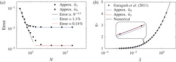
(a) The discrepancy of the zeroth-order solution
 $\tilde{w}_{0}$
and the
 ${\it\delta}$
-correction
 $\tilde{w}_{{\it\delta}}$
compared with the numerical solution versus the number of elements used in the numerical solution
 $N$
. (b) Variation of the scaled fracture width versus
 $\tilde{x}$
for
 ${\it\chi}=0$
(
 $mk$
edge): calculated by Garagash et al. (Reference Garagash, Detournay and Adachi2011) (markers), zeroth-order approximation (blue line),
 ${\it\delta}$
-correction (red line) and the numerical solution (black line).

It is also possible to obtain simple expressions for two out of the three edge solutions, see the parametric triangle in figure 1. To find the approximate solution that corresponds to the
 $mk$
edge (no leak-off), let
 ${\it\chi}=0$
, then (2.21) and (2.23) can be simplified to
 $$\begin{eqnarray}\tilde{w}_{{\it\delta},mk}=(1+3C_{1}({\it\delta})\tilde{x})^{1/3},\quad {\it\delta}={\displaystyle \frac{1}{3}}{\displaystyle \frac{{\it\beta}_{m}^{3}\tilde{x}}{1+{\it\beta}_{m}^{3}\tilde{x}}},\end{eqnarray}$$
while the zeroth-order solution is simply
 $\tilde{w}_{0,mk}=(1+{\it\beta}_{m}^{3}\tilde{x})^{1/3}$
. To find the approximation for the
 $\tilde{m}k$
solution, one can take
 ${\it\chi}\gg 1$
to simplify (2.21) and (2.23) as
 $$\begin{eqnarray}\tilde{w}_{{\it\delta},\tilde{m}k}=(1+4{\it\chi}C_{2}({\it\delta})\tilde{x})^{1/4},\quad {\it\delta}={\displaystyle \frac{1}{4}}{\displaystyle \frac{{\it\beta}_{\tilde{m}}^{4}{\it\chi}\tilde{x}}{1+{\it\beta}_{\tilde{m}}^{4}{\it\chi}\tilde{x}}}.\end{eqnarray}$$
The corresponding zeroth-order solution is
 $\tilde{w}_{0,\tilde{m}k}=(1+{\it\chi}{\it\beta}_{\tilde{m}}^{4}\tilde{x})^{1/4}$
. Unfortunately, it is not possible to extract a simple explicit solution for the
 $m\tilde{m}$
edge from (2.21).
To illustrate the accuracy of the approximate analytical solution, figure 3(a) shows the errors of the zeroth-order approximate solution and the
 ${\it\delta}$
-corrected solution, defined respectively as
 $\max \{|\tilde{w}_{{\it\delta}}-\tilde{w}|/\tilde{w}\}$
and
 $\max \{|\tilde{w}_{0}-\tilde{w}|/\tilde{w}\}$
, where
 $\tilde{w}$
is the numerical solution that is calculated using
 $N$
points in
 $\tilde{x}$
. Here, the maximum is calculated over
 $10^{-8}\leqslant \tilde{x}\leqslant 10^{18}$
and
 $10^{-2}\leqslant {\it\chi}\leqslant 10^{4}$
, which corresponds to the parameter span shown in figure 2. For small values of
 $N$
, the error due to numerical discretization dominates, and one can observe a convergence rate of approximately
 $4$
, which reflects the fact that Simpson’s rule is used to discretize the integral in (2.12). For larger values of
 $N$
, the discretization error becomes smaller than the errors corresponding to the approximate solutions. This leads to an error ‘saturation’, at which the limiting values of the error reflect the accuracy of the approximate solution. The zeroth-order solution,
 $\tilde{w}_{0}$
, has an accuracy of approximately 1.1 %, while the
 ${\it\delta}$
-correction,
 $\tilde{w}_{{\it\delta}}$
, substantially increases the accuracy to 0.14 %. Since the approximate solutions are able to capture all vertex solutions precisely, the error is concentrated in the transition zones. For both approximations, the maximum error is reached in the transition from the
 $k$
to the
 $m$
vertex, which corresponds to
 ${\it\chi}=0$
and
 $\tilde{x}\approx 10^{-1.5}$
. Figure 3(b) shows the variation of the scaled fracture opening versus
 $\tilde{x}$
for
 ${\it\chi}=0$
, i.e. along the
 $mk$
edge. A comparison is made between the numerical solution by Garagash et al. (Reference Garagash, Detournay and Adachi2011), the numerical solution of (2.12), as well as two approximations
 $\tilde{w}_{0}$
and
 $\tilde{w}_{{\it\delta}}$
stemming from (2.24). All solutions agree well with one another, although
 $\tilde{w}_{0}$
is clearly less accurate than
 $\tilde{w}_{{\it\delta}}$
.
3. Buoyancy-driven plane strain fracture
To illustrate the versatility of the approach developed in § 2.2, this section aims to analyse the problem of a buoyancy-driven hydraulic fracture (Spence et al. Reference Spence, Sharp and Turcotte1987; Roper & Lister Reference Roper and Lister2007). As follows from Roper & Lister (Reference Roper and Lister2007), the lubrication equation (2.1), in this case, needs to be replaced by
 $$\begin{eqnarray}{\displaystyle \frac{w^{2}}{{\it\mu}^{\prime }}}\,\left({\displaystyle \frac{\text{d}p}{\text{d}x}}+{\rm\Delta}{\it\rho}g\right)=V,\end{eqnarray}$$
where the leak-off is removed and the
 ${\rm\Delta}{\it\rho}g$
term captures the effect of buoyancy. Here,
 ${\rm\Delta}{\it\rho}$
is the difference between the mass densities of the rock and the fracturing fluid, while
 $g$
denotes the gravitational acceleration. By using a similar procedure to that in § 2.2 (including notation and scaling (2.11)), the analogue of (2.12) becomes
 $$\begin{eqnarray}\tilde{w}(\tilde{x})=1+{\displaystyle \frac{8}{{\rm\pi}}}\int _{0}^{\infty }G(\tilde{s}/\tilde{x})\left[{\displaystyle \frac{1}{\tilde{w}(\tilde{s})^{2}}}-\tilde{g}\tilde{s}^{2}\right]\,\text{d}\tilde{s},\quad \tilde{g}={\displaystyle \frac{{\rm\Delta}{\it\rho}gl^{3/2}}{K^{\prime }}},\end{eqnarray}$$
where
 $\tilde{g}$
is the normalized gravity and
 $l$
is the length scale defined in (2.11). The integral equation (3.2) is solved numerically by using Simpson’s rule to discretize the integral and Newton’s method to solve the system of nonlinear algebraic equations. Since the integral
 $\int _{0}^{\infty }G(\tilde{s}/\tilde{x})\tilde{s}^{2}\,\text{d}\tilde{s}$
does not converge, it is essential to keep both terms under the integral sign in (3.2) together. It should also be noted that an ordinary differential equation similar to (2.19) can be derived from (3.2). Its solution is less accurate (since the assumption
 $\tilde{w}\propto \tilde{x}^{{\it\delta}}$
is no longer valid), but is used as an initial guess for Newton’s method.
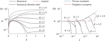
Comparison between the numerical solution of (3.2) (black solid lines) and the numerical solution by Peirce (Reference Peirce2010) (black dashed lines) for the buoyancy-driven hydraulic fracture for different values of
 $K$
. (a) Solutions written in terms of the scaling in Peirce (Reference Peirce2010), see (3.3); the magenta dashed line indicates the approximate solution
 $H_{0}=(X^{1/2}(2-X)^{3/2})/2$
(valid for
 $K\gg 1$
) (Roper & Lister Reference Roper and Lister2007). (b) Solutions written in terms of the scaling (2.11); the blue and red dashed lines indicate the viscous and toughness asymptotic solutions (2.15) respectively. The solution by Peirce (Reference Peirce2010) works poorly for small
 $K$
.

In order to compare the results with the numerical solution (Peirce Reference Peirce2010), which uses a Hermite cubic collocation scheme, we first make a conversion between scaled variables. The normalized fracture toughness,
 $K$
, the normalized fracture half-width,
 $H$
, and the normalized coordinate,
 $X$
, used in Peirce (Reference Peirce2010) are related to our variables as
 $$\begin{eqnarray}K={\textstyle \frac{1}{2}}\tilde{g}^{1/8},\quad H=2^{4/3}\tilde{g}^{1/3}\tilde{x}\tilde{w},\quad X=2^{5/3}\tilde{g}^{2/3}\tilde{x}^{2}.\end{eqnarray}$$
It should be noted that Roper & Lister (Reference Roper and Lister2007) give the asymptotic solution
 $H_{0}=(X^{1/2}(2-X)^{3/2})/2$
(valid for
 $K\gg 1$
) in terms of the aforementioned quantities (3.3). Figure 4(a) compares the numerical solution of (3.2) (black solid lines) with the numerical solution by Peirce (Reference Peirce2010) (black dashed lines) for different values of the normalized fracture toughness
 $K$
. The analytic solution
 $H_{0}$
is represented by the dashed magenta line. Figure 4(b) compares the same solutions, but in terms of the quantities
 $\tilde{w}$
and
 $\tilde{x}$
, and plotted on a log–log scale. The viscous and toughness asymptotic solutions (2.15) are represented by dashed blue and red lines respectively. Both numerical algorithms give nearly identical results for large values of the normalized fracture toughness
 $K$
. At the same time, there is a visible difference for
 $K\leqslant 1$
. This happens because the algorithm in Peirce (Reference Peirce2010) is designed to capture the toughness propagation regime and relies on the toughness asymptotic solution for the tip element; see figure 4(b), where all dashed black lines originate from the toughness asymptote (shown by the dashed red line). The toughness asymptotic solution works poorly in situations when the transition from the toughness to the viscous regime of propagation happens on a length scale comparable to the element size, as indicated in figure 4. At the same time, the new numerical formulation works well for all values of
 $K$
.
4. Summary
This paper introduces an alternative formulation for the multiscale analysis of a steadily propagating semi-infinite hydraulic fracture. The key feature of the approach lies in rewriting the system of governing equations as a single integral equation with a non-singular kernel, whose solution is directly related to the fracture width. This approach is used to provide an accurate numerical solution for a propagating semi-infinite hydraulic fracture with leak-off. Because the new formulation features a non-singular kernel, and does not involve a calculation of the fluid pressure, standard numerical techniques are used to obtain accurate results rapidly. The resulting numerical solution is able to resolve multiscale behaviour and to capture all known asymptotic solutions of the problem. This approach is also used to reduce the problem to an approximate separable ordinary differential equation whose analytic solution captures all known asymptotic solutions of the problem exactly, and provides a highly accurate estimation of the fracture width in transition regions. To highlight the versatility of the new formulation, it is applied to solve the problem of a steadily propagating semi-infinite buoyancy-driven plane strain hydraulic fracture. The results agree well with published numerical solutions that were developed for the toughness-dominated regime of propagation. In addition, the multiscale behaviour at the fracture tip, associated with the transition from the toughness to the viscous regime of propagation, is easily captured using the new formulation.
Acknowledgements
The support of the British Columbia Oil and Gas Commission and the NSERC discovery grants programme is gratefully acknowledged.