Implications
Strategies for combining production and biodiversity conservation in agro-landscapes should consider the diversity of, and interactions between, land uses. Considering a higher level of organisation (e.g. the farm level) increases the range of management options. Putting more effort into the development of agri-environmental policies directed at the farm and landscape levels may be an efficient solution to favour farming systems in which ecology-oriented land uses also make sense from a production point of view.
Introduction
Farmland bird species depend on habitats that cannot be maintained without agricultural activities. Over the last 50 years, however, agricultural intensification has been an important driver of biodiversity loss, and bird species have been particularly affected (Donald et al., Reference Donald, Green and Heath2001). These developments have been particularly apparent in European grasslands, where extensive forms of grazing and mowing are crucial for the maintenance of habitat suitable for grassland bird species (Donald et al., Reference Donald, Pisano, Rayment and Pain2002). Since the early 1990s, public policies (i.e. agri-environment schemes (AES)) have been implemented to compensate the costs resulting from extensive forms of grassland management. This caused a wide-spread adaptation of management practices that aim to promote biodiversity (Ottvall and Smith, Reference Ottvall and Smith2006), but the effects on biodiversity have been below expectations (Kleijn et al., Reference Kleijn, Rundlöf, Scheper, Smith and Tscharntke2011).
Grasslands are, thus, expected to fulfil the two-fold objective of agricultural production and biodiversity conservation. A large number of studies have addressed these objectives at the field scale (Durant et al., Reference Durant, Tichit, Kernéïs and Fritz2008). At this level, production and conservation often seem to conflict; high levels of biodiversity are difficult to achieve under the most intensive farming practices (Plantureux et al., Reference Plantureux, Peeters and McCracken2005). The main perspectives for the reconciliation of ecological conservation and agricultural production require adjustment of the timing, frequency and intensity of grazing or mowing regimes. For example, the results of several studies of grassland birds suggest that decreasing or increasing livestock densities at specific times of the year is a key management tool for conservation (Tichit et al., Reference Tichit, Doyen, Lemel, Renault and Durant2007). Other studies highlight that decreasing mowing frequency and postponing mowing dates can favour grassland bird species (Kruk et al., Reference Kruk, Noordervliet and Ter Keurs1996).
Underlying mechanisms that link management practices with bird life cycles operate through direct and indirect effects (Durant et al., Reference Durant, Tichit, Kernéïs and Fritz2008). Direct effects include nest or juvenile destruction via mowing and trampling by cattle (Labinsky, Reference Labisky1957; Beintema and Muskens, Reference Beintema and Muskens1987). Indirect effects originate from the control of habitat quality (e.g. creation of suitable grass height during chick rearing; Tichit et al., Reference Tichit, Doyen, Lemel, Renault and Durant2007; Durant et al., Reference Durant, Tichit, Kernéïs and Fritz2008).
In addition to these field-level studies, an increasing number of studies highlight the importance of higher levels of organisation when considering both production and ecological conservation objectives in agricultural areas (Groot et al., Reference Groot, Jellema and Rossing2010; McMahon et al., Reference McMahon, Helden, Anderson, Sheridan, Kinsella and Purvis2010). At these higher levels of organisation, interactions between system components result in system behaviour that is not apparent when only the field level is considered. From the ecological perspective, birds benefit from complementation between resources (Brotons et al., Reference Brotons, Wolff, Paulus and Martin2005), and the diversity of land uses within the landscape is a key driver of biodiversity (Benton et al., Reference Benton, Vickery and Wilson2003). From the production perspective, the farm is a management and an economic unit, and therefore should be included in intervention-oriented studies. Management practices applied to different fields on a farm are inter-related, as together they serve farm-level goals (e.g. year-round feed provisioning; Martin et al., Reference Martin, Hossard, Theau, Therond, Josien, Cruz, Rellier, Martin-Clouaire and Duru2009). Farm level is, therefore, a relevant level for environmental management, as shown by a few AES implemented at the farm (e.g. the OLAE in France in the 90s; Havet et al., Reference Havet, Pons and Kerneis2005) or at the landscape (e.g. mosaic management in the Netherlands; Shekkerman et al., Reference Schekkerman, Teunissen and Oosterveld2008) levels. However, these types of AES are not widely used, and most schemes have been implemented at the field level.
The objective of this study was to investigate how an AES implemented at the farm level would shape the relationship between production and ecological performance. More precisely, we used a dynamic model of a grassland agro-ecosystem to assess how different ecological constraints (defined at field and farm level) affected ecological and production performance. The study focussed on interactions between production and bird ecology at the farm level. It was based on a model of grassland productivity at field and farm levels, which was linked to a bird population dynamics model that included habitat preferences. We applied the mathematical framework of viability theory to the model (Aubin, Reference Aubin1991), which made it possible to identify the sets of management strategies that respect a given set of constraints. This framework was particularly suited to our study, because it addressed the problem faced by a farmer searching for viable management strategies under a set of environmental, biotechnical and regulatory constraints (Tichit et al., Reference Tichit, Hubert, Doyen and Genin2004; Baumgartner and Quaas, Reference Baumgärtner and Quaas2009). Compared with previous applications of the viability theory, our study was novel because we incorporated constraints defined at both the field and farm levels, and we jointly accounted for three types of constraints. The first type related to production (e.g. biomass available for cattle), the second type related to the ecology of two bird species (e.g. suitable grass heights for birds in one of the land used) and the third type related to environmental regulation (e.g. a minimal share of the land managed for bird conservation). We parameterised the model with data from the Marais Poitevin wetland in France and for two different bird species – the northern lapwing (Vanellus vanellus) and the common redshank (Tringa totanus) – with distinct habitat requirements. Given the explorative aim of the study and the need for the viability approach, the model was parameterised to produce recognisable system dynamics, rather than to provide output for prediction purposes.
To test for a ‘farm type’ effect and assess for which farm type the use of AES would be the most efficient, we first drew the relationship between ecological and production performance in two contrasting types of grassland-based farms. These intensive and extensive farms corresponded to the two extreme types of farms found in our study area. We also examined more precisely the characteristics of the different management strategies at the field level.
Material and methods
Conceptual model
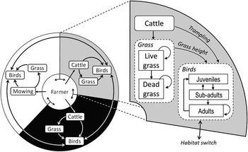
We built a spatially implicit state-control model that described the dynamics of a suckling farm based on permanent grasslands. A monthly time step was used. Grasslands were a feed resource for cattle and breeding habitat for two wader species. The model captured two levels of organisation (field and farm) and two objectives (grassland productivity and stability of the bird populations). It was used to compare two farm types (intensive and extensive farms) that differed in stocking rates at the field and farm levels. The model linked management decisions to grass and bird dynamics at the field and farm levels (Figure 1).
Conceptual model of the livestock farming system. Management decisions involved (i) proportion of land use alternatives at the farm scale (production-oriented grazing in black, ecology-oriented grazing in grey and mowing in white); (ii) timing and intensity of grazing or mowing. Bird dynamics were mainly directly affected by nest trampling by cattle, and indirectly affected by grass height, which determines habitat selection and juvenile survival.

At the farm level, management reflected the farmer’s decisions regarding the proportion of the area under three types of land use: mowing (MOW), production-oriented grazing (POG) and ecology-oriented grazing (EOG). MOW corresponded to the harvest of grass once per year at the end of May to provide forage for feeding cattle indoors. EOG corresponded to grazing sequences aimed at generating a habitat of good quality and limiting nest trampling in spring for each of the two wader species. POG corresponded to high grazing intensities maximising the grass harvested by cattle without any ecological constraint. The proportions of the three land uses affected farm feed self-sufficiency. These proportions also defined the amount of habitat potentially suitable for each bird species through time and their options for switching habitat. Specification of mowing and grazing intensities were defined for each land use. At this level, decisions on timing, duration and amount grazed were not defined a priori, but resulted from a dynamic optimisation process.
The optimisation algorithm was based on the mathematical framework of viability theory (Aubin, Reference Aubin1991), which enabled identification of a set of decisions that maintained the suckling farm system within a set of constraints that defined the farm’s production and ecological sustainability. These decisions modulated the dynamics of grassland productivity and the effect on bird dynamics, both directly through nest trampling and indirectly through its effects on grass height and, consequently, juvenile survival. Management decisions at the farm and field levels were, thus, driving forces of production and ecological performance. We ran a single viability algorithm that included the field and farm levels and the two bird species simultaneously. The next sections provide descriptions of key model equations at, consecutively, the farm and field levels (vectors indicated in bold font). A complete description of the model (including detailed description of matrixes A, M, R and functions H, f and s 0) is given in Supplementary Material S1.
The decision sub-system
The relative proportions of the three grassland land uses at the farm level are fixed at the start of each year, as described by the vector p t :
 $$p_{t} =\left( {\matrix{ {p_{t}^{{{\rm MOW}}} } \cr {p_{t}^{{{\rm POG}}} } \cr {p_{t}^{{{\rm EOG}}} } \cr } } \right)$$
At the beginning of each month, a decision is made on the stocking rate (in livestock units per hectare, LU/ha),
u
t
=(
 $$u_{t}^{{{\rm MOW}}} ,\,u_{t}^{{{\rm EOG}}} ,\,u_{t}^{{{\rm POG}}} $$
)’, allocated to the different land uses (the symbol ’ indicates transposition). Values of
u
t
are limited by u
tot, an upper threshold reflecting the stocking rate at the farm level. Two farm types, intensive and extensive, were compared. They differed in two characteristics, the stocking rate at the farm level (u
tot) and the maximum stocking rate in POG. When the entire herd could not be fed grazed biomass, fodder from mown fields was used for supplementation.
The biotechnical sub-system
Grass dynamics
Model of grass dynamics is an adaptation of the model developed by Tichit et al. (Reference Tichit, Doyen, Lemel, Renault and Durant2007). The dynamics of grass growth and death are simulated at a monthly time step. In each land use j, grass biomass
 $B_{t}^{j} $
is partitioned into live and standing dead grass – that is,
 $B_{t}^{j} $
=(
 $$B_{{_{{L,t}} }}^{j} ,B_{{D,t}}^{j} $$
)’ expressed in organic matter per square meter (g OM/m²), which grows, senesces and/or decays.
 $B_{t}^{j} $
is affected by grazing and mowing:
 $$B_{{t{\plus}{\rm 1}}}^{j} =A(t,B_{t}^{j} )B_{t}^{j} {\minus}H_{t}^{j} (u_{t}^{j} ,B_{t}^{j} )$$
In equation (2),
 $$H_{t}^{j} $$
represents biomass harvest by mowing (j=MOW) or grazing (j=EOG,POG) in g OM/m2. Matrix A describes the rates of increase and decrease of living and dead standing grass. Matrix A is composed of the three following transition rates: growth, senescence and decay.
Bird dynamics
The bird dynamic model is a spatial adaptation of the model by Sabatier et al. (Reference Sabatier, Doyen and Tichit2010). Population dynamics of each wader species are represented as staged structured matrix models with three classes – juveniles, sub-adults and adults (suffixes 0, 1 and 2). Each population is divided into three sub-populations, each corresponding to one of three land uses (MOW, POG or EOG). The population of each species is described by a (9×1) vector, N t :
 $$\eqalignno{N_{t} =\left ( {N_{{t,0}}^{{{\rm MOW}}} ,N_{{t,1}}^{{{\rm MOW}}} ,N_{{t,2}}^{{{\rm MOW}}} ,N_{{t,0}}^{{{\rm POG}}} ,N_{{t,1}}^{{{\rm POG}}} ,N_{{t,2}}^{{{\rm POG}}}}\right , \cr \left N_{{t,0}}^{{{\rm EOG}}} ,N_{{t,1}}^{{{\rm EOG}}} ,N_{{t,2}}^{{{\rm EOG}}} } \right)'$$
with
 $N_{{t,i}}^{j} $
being the density of birds of age class i, and subject to land use j, at time t.
Wader dynamics from time, t, to time, t+1, is described using
 $$N_{{t{\plus}1}} =M_{t} \left( {h_{t} ,p_{t} ,u_{t} ,N_{t} } \right)R_{t} \left( {h_{t} ,p_{t} } \right)N_{t} $$
where M
t
is the demographic matrix, R
t
the habitat selection matrix and
 $$h_{t} =\left( {h_{t}^{{{\rm MOW}}} ,h_{t}^{{{\rm EOG}}} ,h_{t}^{{{\rm POG}}} } \right)$$
’ the grass height at time t, expressed as
 $$h_{t}^{j} =a(B_{L}^{j} {\plus}B_{D}^{j} )\quad \quad j={\rm POG},{\rm EOG},{\rm MOW}{\rm }$$
The two matrixes, M t and R t , account for class and spatial fluxes, respectively. The habitat selection matrix, R t , addressed selection of nesting sites by adults, and selection of foraging habitat by juveniles. Selection of habitats by birds depends on grass height in the different land uses. Matrix M t describes traits of the bird species, and the direct and indirect effects of grassland management regime. It accounts for clutch size, f, which depends on trampling by cattle, and juvenile survival, s 0, which depends on grass height.
Performance indicators
Two indicators were computed for production performance at the farm level, harvested grass and feed self-sufficiency. Harvested grass was calculated as the yearly average of total biomass from grazing and mowing (g OM/m2 per year):
 $${\rm Harvested}\,{\rm grass}={1 \over Y}\mathop{\sum}\limits_{t=1}^T {\left( {\mathop{\sum}\limits_{j\in \left[ {{\rm EOG,POG,MOW}} \right]} \!\!\!\!\!\!\!\!\!\!\!{p_{t}^{j} H_{t}^{j} } } \right)} $$
with Y=T/12 the number of years to horizon.
The second indicator was feed self-sufficiency, which was expressed as the yearly average share of herd feeding requirements covered by the farm grasslands:
 $${\rm Feed}\;{\rm self{-}sufficiency}=100{{{\rm Harvested}\,{\rm grass}} \over {12Yq\,u_{{{\rm tot}}} }}$$
where u tot was stocking rate at farm level expressed in LU/ha, and q was the monthly feeding requirement of one livestock unit (g OM/lU per month). We implicitly assumed that when cattle were not grazing, they were kept indoors and were fed with external resources.
Two indicators of ecological performance were also computed, respectively, at the field and farm levels. At the farm level, we recorded the yearly average population growth rate:
 $${\rm Population}\,{\rm growth}\,{\rm rate}={{N_{T} {\minus}N_{0} } \over {YN_{0} }}$$
with N T the population size at time T.
At the field level, we computed the expected reproductive success as the product of juvenile survival, s 0, and clutch size, f (see Supplementary Material S1 for the definition of f and s 0):
 $${\rm Reproductive}\,{\rm success}^{j} =f^{j} s_{0}^{j} $$
for j ∈ [MOW, POG, EOG].
Calibration
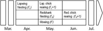
The grass sub-model was calibrated using data from our study area: the Marais Poitevin, France (46°22′N, 1°25′W). The bird sub-model was calibrated using data published on the two most abundant wader species of our study area, the northern lapwing and the common redshank. These two bird species represented contrasting ecological requirements, and their life cycles do not coincide (Figure 2).
Timeline of the bird life cycles and farming activities.

Details of the calibrations and parameter values are presented in Supplementary Material S2.
Viability constraints
We defined six constraints at field and farm levels that together secured the viability of the farming system. Stocking rate was bounded by a lower and upper limit so that grazed biomass could not exceed the locally available biomass, and the total number of grazing animals could not exceed the farmer’s herd size. Grass height and stocking rate had an upper bound in EOG to ensure good ecological performance for each bird species. At the farm level, a threshold was set on the proportion of EOG.
The first constraint defined the minimum proportion of farm area allocated to EOG, p (−):
 $$p_{t}^{{{\rm EOG}}} \gt p^{{\left( {\minus} \right)}} $$
In management terms, p (−) could represent the area of the farm devoted to AES.
The second constraint imposed an upper limit on the maximum stocking rate allowed on the farm:
 $$\mathop{\sum}\limits_{j\in \left[ {{\rm EOG,POG}} \right]} {p_{t}^{j} u_{t}^{j} \leq u_{{{\rm tot}}} } $$
The third constraint imposed an upper limit on stocking rate in POG for each farm type (with u (+) differing between intensive and extensive farms):
 $$u_{t}^{{{\rm POG}}} \leq u^{{({\plus}),{\rm POG}}} $$
The fourth viability constraint limited stocking rate at time, t, so that grazed biomass, qu, could not exceed available resource:
 $$q\,u_{t}^{j} \leq B_{{Av,t}}^{j} \left( {B_{t}^{j} } \right)\,{\rm for}\,j=\left( {{\rm EOG},{\rm POG}} \right)$$
with
 $$B_{{Av,t}}^{j} $$
the grass biomass available for grazing, considering that cattle could not graze at sward heights <5 cm.
The final two constraints restricted the management of EOG such that it resulted in an optimal habitat for the two wader species while limiting nest trampling. One constraint limited the effect of trampling on the egg survival rate during the egg incubation period, and imposed an upper threshold, u (+), on stocking rate during the nesting month, (t*):
 $$u_{t}^{{{\rm EOG}}} \leq u^{{\left( {\plus} \right),{\rm EOG}}} \,\,\,\,\,\,t=t{^\asterisk}{\plus}k,{\rm }k=1,...,K{\minus}1$$
with K=T/12, the number of year to time horizon.
To ensure maximum juvenile survival, the other constraint imposed a lower and upper limit on grass height during the month following hatching, (t*+1), for each species:
 $$h^{{\left( {\minus} \right)}} \leq h_{{t{\asterisk}{\plus}1}}^{{{\rm EOG}}} \leq h^{{\left( {\plus} \right)}} $$
Constraints (14) and (15) were defined for both bird species.
Viability analysis
The identification of viable combinations of grass biomass, B , grazing intensity, u , and proportion of management regimes, p , corresponded to the computation of the viability corridor, Viab t . At time t=t 0, Viab t was defined as the set of initial states, {B t 0 }, such as there existed combinations of controls, u t , p t and states, B t , starting from B t 0, satisfying constraints (10), (11), (12), (13), (14) and (15) for any time t=t 0, … , T.
After the viability corridor was determined, we computed the set of viable management strategies, U v , which matched the viability constraints. A viable management strategy, U v =[u t , p t ], existed as long as the corresponding state, B t , was within the viability corridor, Viab t . The set of viable controls at time, t, for a given viable grass state, B t , was
 $$\eqalign{U_{{V,t}} (B_{t} ) =\cr \left\{ {(u_{t} ,p_{t} )\left| {\matrix{ {{\rm constraints}\;\left( {10} \right),\left( {11} \right),\left( {12} \right),\left( {13} \right),\left( {14} \right)\;{\rm are}\;{\rm satisfied}} \cr {A_{t} (B_{t}^{j} )B_{t}^{j} {\minus}H(u_{t}^{j} ,B_{t}^{j} )\in \;{\rm Viab}_{{t{\plus}1}} \;{\rm for}\;j={\rm EOG,POG,MOW}} } \right} \right\}$$
Following the approach of Doyen and de Lara (Reference Doyen and De Lara2010), dynamic programming was applied for numerical approximation of Viab t and U v .
Simulations
The viability algorithm was run over a time period of T=120 months to capture the long-term ecological dynamics while remaining coherent from the farming perspective. The viability algorithm was run simultaneously for the two bird species in each of the two farm types. Different values of the p EOG oriented constraint (p (−) ranging from 0% to 40% with a 5% interval) were explored so as to reflect increased ecological concern. Farm types differed with regard to the maximum field level stocking rates in POG (u (+),POG=1.5 in extensive and 4.5 LU/ha in intensive farms) and farm level stocking rates (u tot =0.84 in extensive and 2.06 LU/ha in intensive farms). For each simulation, the algorithm computed the proportions of mowing, POG and EOG, as well as the corresponding grass dynamics. Within the set of viable management strategies, the viability algorithm extracted the strategies that maximised the harvested grass indicator that reflected the production objectives of the farmer. For each simulation, the performance indicators (grassland production, farm self-sufficiency and bird population) were computed.
Dynamics showed periodic patterns after 1 year of regime establishment: Viab t+12=Viab t , constant values of p , 12-month periodicity for u and B and a monotonous trend for N. Long-term dynamics were only sensitive to N 0 that was parameterised at N 0=100 for both bird species. Given this dependency on initial conditions, the ecological indicators were expressed in relative terms (i.e. relative to N 0). All computations were performed using Scilab 4.1.2 software (http://www.scilab.org; Scilab Consortium 2007).
Results
Production–conservation trade-offs at farm level
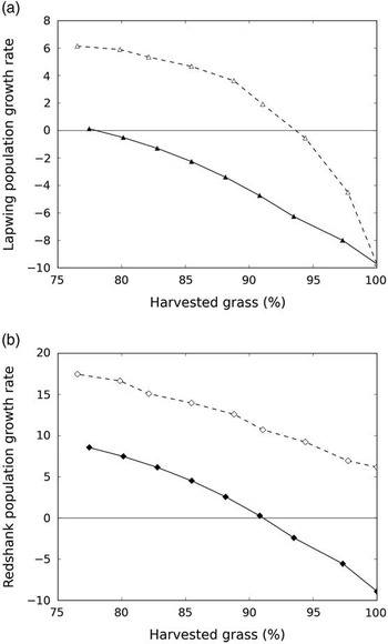
The model simulation results indicated that wader bird population growth rates (ecological performance) and harvested grass (production performance) could not be maximised simultaneously (Figure 3). A trade-off emerged in which any ecological improvement involved a production loss, and vice versa. The shape of the trade-off curve was concave (especially clear for the lapwing), which indicated that ecological performance of a farm with average grassland production was higher than the average ecological performance of the two extreme farms. In other words, a farm that combined production and ecology outperformed a combination of two systems focussed on only a single criterion. The trade-off curve differed between intensive and extensive farms for both bird species, which indicated the presence of a farming system effect. In terms of production loss, achieving high ecological performance on extensive farms was less costly compared with intensive farms. For example, maintaining lapwing populations at their initial level resulted in a 6% decrease in total harvested grass on extensive farms, and a 22% decrease on intensive farms.
Trade-off between harvested grass and the lapwing (a) or the redshank (b) population growth rates on different farm types: intensive (continuous line) and extensive (dashed line). Each point represents a set proportion of ecology-oriented grazing (EOG). For each farm, harvested grass was set to 100% when no area was allocated to EOG.

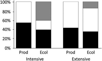
In terms of proportion of land uses (Figure 4), maximisation of harvested grass resulted in an almost equal allocation of the area to mowing and POG. Maximisation of production also resulted in, logically, 0% of the area allocated to EOG. To maintain bird populations, intensive farms had to allocate more area to EOG (i.e. 40% of the farm area v. 15% on extensive farms).
Proportions of the different land uses in the two types of farms for two objectives, maximising production (prod) and maintaining bird populations (ecol). White: mowing, black: production-oriented grazing, grey: ecology-oriented grazing.

Production performance
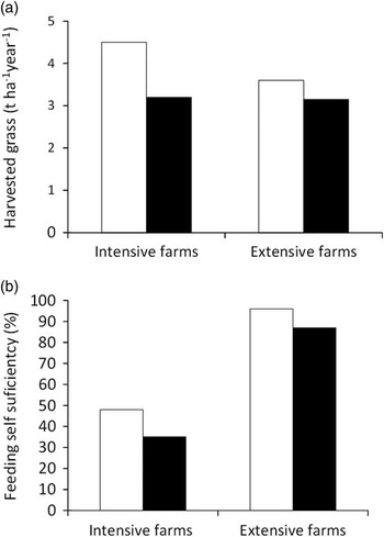
Harvested grass depended on the farm type and on the proportion of land uses (Figure 5a). Maximum forage production levels on intensive farms were around 30% greater compared with extensive farms. They averaged 4.5 and 3.3 t/ha per year for intensive and extensive farms, respectively. When bird populations were maintained, however, intensive and extensive farms achieved overall similar yields (3.2 and 3.1 t/ha per year, respectively), but the allocation of the different land uses was different (Figure 4). The greater cost for intensive farms to move from a production-first orientation to an orientation allowing co-existence of production and ecology was due to the need to dedicate more area to EOG.
Average harvested grass (grazing and mowing) (t/ha per year) at the farm level (a) and feed self-sufficiency (b) of an intensive and an extensive farm, assuming maximising production (white bars) and maintaining bird populations (black bars).

Intensive and extensive farms were very different with respect to the feed self-sufficiency ensured by grazed and mowed forage. Regardless of the mix of grassland management regimes, grasslands provided almost 100% of the cattle feeding requirements on the extensive farm (Figure 5b). Conversely, the intensive farm achieved only 50% self-sufficiency, and this percentage decreased when ecological constraints were increased. Intensive farms hosted a higher stocking rate (u tot) and relied more on external feed resources.
Ecological performance
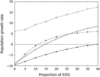
At the farm level, the proportion of EOG was a stronger driver of population growth rates than the farm type, especially for lapwings (Figure 6). Beyond this first factor, the type of farm also explained population growth rates. Extensive farms had better ecological performance than intensive farms; for the same proportion of EOG, bird populations had higher growth rates (Figure 6). In most cases, without EOG, bird populations had strong negative growth rates, and these rates were positive only when EOG was above a specific threshold. However, on extensive farms, redshank populations increased even without EOG. This result can be explained by differences in agro-ecological dynamics at the field level, as explained in the next section.
Bird population growth rates of the lapwing (triangle) and the redshank (diamonds) for increasing proportions of EOG in intensive farms (continuous line) and extensive farms (dashed lines).

Underlying mechanism at the field level
Grazing sequences
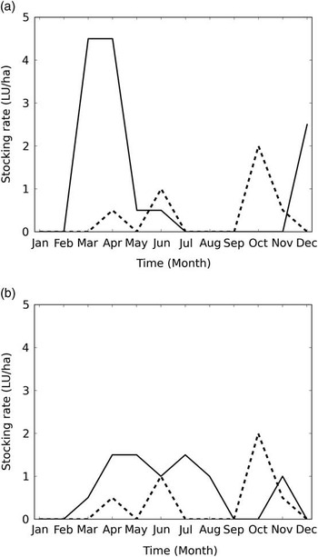
Grazing patterns in EOG remained the same from one farm to the other. Only POG differed between the intensive and the extensive farms. In POG, timing and intensity of grazing differed between the intensive and the extensive farms (Figure 7). The model predicted a stocking rate of 4.5 LU/ha during mid-spring (April and May) on the intensive farm, when the highest grass growth rates occurred. Compared with the intensive farm, mid-spring stocking rates (April to May) were much lower on the extensive farm (60 LU days/ha on extensive farms v. 270 LU days/ha in intensive farms), and grazing was more homogeneously spread from March to August. Stocking rates ranged from 0.5 to 1.5 LU/ha on extensive farms, and they peaked at 4.5 LU/ha on intensive farms. These differences in timing of grazing resulted in the model predicting that cattle would be kept indoors longer on intensive farms (5 months) compared with extensive farms (4 months), during the winter and summer periods.
Monthly stocking rate during one year in the two types of farms: (a) intensive and (b) extensive. The two grazing regimes shown (full line: production-oriented grazing, dashed line: ecology-oriented grazing) maximise harvested grass at the farm level while respecting the different constraints.

POG on the intensive farm resulted in a high total grazed biomass (4.6 t/ha per year), whereas grazed biomass was 3.0 t/ha per year on the extensive farm. EOG resulted in 1.5 t/ha per year of grazed biomass for both farm types.
Ecological performance of the land uses
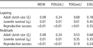
The land uses had contrasting effects on bird life history parameters (Table 1). As expected, EOG provided the best habitat, with very low levels of trampling. Mowing and POG on intensive farms led to the lowest reproductive success.
Value of life history parameters for the two bird species and the different land uses

MOW=mowing; POG (int.)=production-oriented grazing in intensive farms; POG (ext.)=production-oriented grazing in extensive farms; EOG=ecology-oriented grazing.
On extensive farms, POG was associated with moderate stocking rates during the nesting months, and induced limited nest trampling for both species (Figure 7). These moderate stocking rates induced moderate grass heights that were suitable for the redshanks, but too tall for the lapwings. For conservation of the redshank, managing grasslands with a moderate stocking rate is, therefore, suitable for both habitat quality and limiting trampling. This result provides an explanation for the relatively high redshank reproductive success during POG on extensive farms.
Discussion
We developed a spatially implicit dynamic model to investigate the consequences of farmers’ grassland management decisions on the dynamics of grassland production and the dynamics of two wader populations on suckling farms. Production and ecological performances showed a concave trade-off curve that depended on farm intensification level. Diversity of land uses was a key factor for the maintenance of harvested grass and bird population sizes at high levels. Maintaining viable populations was less costly for the redshank compared with the lapwing populations. This result indicated that, depending on the target species and the production context, ecological performance was compatible with production.
Model objectives and limitations
We aimed to develop a model that produced recognisable and realistic patterns of grass and bird dynamics at the field and farm levels, so that the dynamics of contrasting farm types could be compared. The model was quite detailed, but relied on several simplifying assumptions that should be discussed.
The model was deterministic
It, therefore, did not account for uncertainty on parameter values or for variability in environmental conditions. Including stochasticity on key parameters (e.g. grass dynamics or bird demography) would be an approach to overcome both limitations. Stochastic viability algorithms have been developed (Doyen and de Lara, Reference Doyen and De Lara2010), but are very time and memory consuming and could not be used with our model. We did, however, test the range of validity of our results by focussing on two bird species with contrasting ecological needs and on two farm types that represented the lower and higher farming intensities of our study area.
In contrast to a previous study that focussed on the effects of landscape structure on bird dynamics (Sabatier et al., Reference Sabatier, Doyen and Tichit2014), this model emphasised production-related interactions within a farm and included a spatially implicit representation of chick dispersal. Manipulating the spatial configuration of land use is an important way to reconcile production and ecological objectives. However, spatial configuration is difficult to implement at the farm level because farm area is usually not contiguous, and land use allocation depends on a wide range of external constraints that limit the farmers’ options (e.g. accessibility of machinery to the field or distance to the farm (Andrieu et al., Reference Andrieu, Josien and Duru2007)).
Opting for an implicit representation of space limited the complexity of the model, which allowed us to run simulations within the viability theory framework. With viability theory, land uses were not defined a priori, but resulted from a dynamic optimisation under constraints. By optimising grazing management, we likely over-estimated the amount of grass harvested by grazing. It is also likely that, in practice, the farmer does not reach this optimal situation and under-exploits the biomass because of lack of information about the amount of available biomass, or because non-production objectives prevail (e.g. using land for young or diseased stock). This over-estimation of grazing was confirmed by the field data. In the study site, average cumulated stocking rate in grazed fields was 233 LU days/ha, whereas our model predicted 375 LU days/ha in POG (and 225 LU days/ha in EOG). However, this lower production does not imply better ecological performance, because only 2% of the fields provided suitable grass heights and grazing intensities for the lapwings (Sabatier et al., Reference Sabatier, Doyen and Tichit2010).
Importance of ecological interactions between land uses
Our results suggested that strategies for combining production and conservation should consider land use diversity and interactions. Green et al. (Reference Green, Cornell, Scharlemann and Balmford2005) proposed a conceptual model focussed on the trade-off between production and biodiversity in agro-landscapes managed with different strategies of spatial allocation of land use. In their model, the performance of a landscape composed of two management regimes was the average of the two regimes, thus assuming a linear effect of the proportion of land use and the absence of interaction. Other authors have discussed the importance of accounting for interactions between management regimes, such as the negative effects of production-oriented land use, on the conservation-oriented area (Vandermeer and Perfecto, Reference Vandermeer and Perfecto2005). Our results revealed a non-linear effect of the proportions of land use, thus highlighting the importance of such interactions. In our case, this interaction was related to the capacity of birds to select habitat at different stages of their life cycles, and to, therefore, benefit from ecological complementation (Brotons et al., Reference Brotons, Wolff, Paulus and Martin2005).
Implications for conservation in agro-landscapes
In addition to this ecological interaction, our model illustrates the importance of production-related interactions within the farming system. EOG made it possible for livestock to graze in October, a month where grazing did not occur on production-oriented fields. This result shows how synergies can be found between production and ecological goals, as soon as the production dimension is considered beyond the maximisation of grass biomass production. The importance of such alternative functions strongly depends on the farmer’s global strategy, defined at the level of the farming system. This suggests that changing the target of AES from field to farm may be an efficient solution to favour farming systems in which ecology-oriented land uses would also make sense from a production perspective.
In addition to the effects of complementarity between land uses, our results indicated that there was an effect of the overall intensity of the farm on bird population levels. This effect was noticeable for the redshank, for which the population could be maintained on extensive farms, even without EOG. This result can be explained by the contrasting ecological requirements of the lapwing and the redshank. The lapwing has very specific requirements. It requires short grass and, therefore, heavily grazed pastures; however, it is sensitive to nest trampling during the most productive grazing period. The life cycle of the redshank begins later in the year and this species nests at higher grass heights. Its ecological requirements are, thus, compatible with a wide range of extensive forms of grazing, which explains why it benefited from the POG in extensive farms in our simulations.
Our results indicating the presence of a farm effect on the production–conservation trade-off support the results of empirical studies reporting a farming system effect on biodiversity (McMahon et al., Reference McMahon, Helden, Anderson, Sheridan, Kinsella and Purvis2010). It is also congruent with studies that advocate agri-environment scheme implementation at the farm level (Marini et al., Reference Marini, Fontana, Battisti and Gaston2009). More precisely, our results indicated that, with similar investments, conservation outcomes were higher for an extensively managed farm. Allocating resources where they provide the highest environmental benefit is crucial to improve the cost-effectiveness of conservation actions (Teillard et al., Reference Teillard, Allaire, Cahuzac, Léger, Maigné and Tichit2012). Our results are consistent with other studies suggesting that conservation actions yield higher biodiversity benefits in extensive farms or regions (Kleijn and Sutherland, Reference Kleijn and Sutherland2003). Beyond agricultural areas, resource allocation based on cost-effectiveness is also crucial for patrimonial or threatened species conservation (Joseph et al., Reference Joseph, Maloney and Possingham2009).
Conclusion
Our model was the first to link dynamic modelling approaches at the field and farm levels to assess ecological and production performance of a livestock farming system. Our results revealed the presence of a farming system effect and a concave trade-off between the two performances. These results were outcomes of interactions between production-oriented and ecology-oriented land uses within the farming system. Multi-objective grassland management would benefit from public policies that consider levels of organisation higher than the field level.
Acknowledgements
This work was carried out with the financial support of the Agence Nationale de la Recherche, the French National Research Agency, under the SYSTERRA program’s Ecosystems and Sustainable Development (project ANR-08-STRA-007, FARMBIRD – Coviability models of FARMing and BIRD biodiversity).
Supplementary material
To view supplementary material for this article, please visit http://dx.doi.org/10.1017/S175173111400281X