

1 Introduction
It has often been observed that sound systems are structured in a way that minimises the perceptual confusion between its elements. For instance, a language with only three vowels tends to keep them far apart in the two-dimensional space of the auditory first and second formants, i.e. such a language tends to pronounce them as sounds close to the ‘corner’ vowels [a i u]. A related observation is the existence of chain shifts in sound change. For instance, a change of a vowel pronounced [u] into a vowel pronounced [y] is often followed by a change of [o] into [u], filling up the corner just vacated; or the consonants pronounced [dɦ d t] in Proto-Indo-European have shifted to [d t Ɵ] in Germanic and on to [t ʦ d] in German. In all these shifts, the common theme is that the contrast between the members of the inventory is maintained, although all members change. At the abstract level of the language, therefore, it appears that languages actively strive to implement an optimal auditory dispersion and to maintain this dispersion diachronically.
At the same time, many authors insist that perceptually based sound change can only take place by innocent misapprehension, i.e. that speakers do not have the perceptual optimisation of a sound system as a goal but that sound change is instead caused by learners who reanalyse the imperfectly transmitted sounds of their language environment (Ohala Reference Ohala, Masek, Hendrick and Miller1981, Blevins Reference Blevins2004).
There seems to be a tension between the idea of optimal auditory dispersion and the idea of innocent misapprehension. A proponent of auditory dispersion even claims that ‘sound change through misperception … can only hope to account for neutralization, not dispersion or enhancement’ (Flemming Reference Flemming, Pisoni and Remez2005: 173). This is not entirely true: there may exist non-goal-oriented mechanisms by which improvement of auditory contrast could be a common but unintended result of innocent misapprehension. For instance, Blevins (Reference Blevins2004: 285–289) tentatively explains chain shifts with the help of Pierrehumbert's (Reference Pierrehumbert, Bybee and Hopper2001) claim that exemplar theory predicts automatic shifting of auditory vowel prototypes to regions where they are less likely to be perceived as a different category (see §7.2). All authors agree, however, that formalising auditory dispersion with existing formal phonological devices such as Optimality Theory (OT) is incompatible with the claim of innocent misapprehension. Thus, the OT accounts of dispersion of Flemming (1995, Reference Flemming2004), Padgett (Reference Padgett, Hume and Johnson2001, Reference Padgett2003a, Reference Padgettb, Reference Padgett2004) and Sanders (Reference Sanders2003) contain explicitly goal-oriented elements, namely dispersion constraints.
The present paper reconciles auditory dispersion with innocent misapprehension without resorting to exemplar theory. We show that in the other main neurologically informed linguistic framework, namely constraint grammars (stochastic OT, noisy Harmonic Grammar, Maximum Entropy), auditory dispersion does turn out to emerge mechanically as long as we assume bidirectionality, i.e. that a language user applies the same constraint rankings (or weights) to perception and production. We thus show that the innocent misapprehension standpoint can be correct in stating that speakers are not goal-oriented, while at the same time the auditory dispersion standpoint can be correct in observing that sound change tends to minimise perceptual confusion. The reconciliation will be seen to derive from the possibility that sound change is teleological at the abstract level of the observed language, but non-teleological at the concrete level of the language user; this situation is analogous to that in evolutionary biology (Darwin Reference Darwin1859), where adaptations to the environment are observationally optimising but underlyingly non-teleological.
This paper is structured as follows. In §2 we provide an overview of dispersion effects, and briefly discuss earlier accounts of them. In §3 we introduce the bidirectional grammar model that we need for our own non-teleological explanation of dispersion. In §4 we introduce the specific case considered in this article, sibilant dispersion. In §§5 and 6 we provide computer simulations of the acquisition of sibilant inventories, which show that non-dispersed inventories can be learned to some extent but will automatically change within a few generations into dispersed systems that will stay stable over any following generations. In §7 we discuss the necessary assumptions in our model and compare them with those of previous models. We end by concluding that dispersion effects are intrinsic to bidirectional constraint-based grammar models, so that we predict analogous effects operating at all levels of the grammar.
2 Auditory dispersion effects and explanations
In this paper we confine ourselves to the simplest case of dispersion, namely the one-dimensional case. In this section we first present six kinds of dispersion effects, then discuss earlier accounts from the non-OT and OT literature.
2.1 Six kinds of auditory dispersion effects
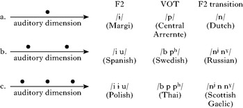
In Fig. 1 we see examples of how phonological categories can be dispersed along one-dimensional auditory continua. This figure helps us to illustrate the six kinds of dispersion effects. Most languages tend to be dispersed like the cases we discuss here; cases of real or apparent undispersed inventories are discussed at the end of this section.
Observed auditory dispersion.

2.1.1 The preference for the centre
If a language has only one category on the continuum, it tends to be in the centre (Fig. 1a). We know this because it tends to have the same auditory value as the mid value of an inventory with three phonemes on the continuum (Fig. 1c). For instance, languages with only one category on the continuum of voice onset time (VOT) for plosives, such as Central Arrernte (Breen & Dobson Reference Breen and Dobson2005), typically have only the zero VOT value, as in the plain voiceless plosive [p],Footnote 1 while languages with three categories, such as Thai (Tingsabadh & Abramson Reference Tingsabadh and Abramson1999), typically have a ‘prevoiced’ [b] (negative VOT), [p] (zero VOT) and an aspirated [p&phosuph;] (positive VOT). Likewise, languages with only one high vowel, such as Margi (Maddieson Reference Maddieson1987) or Kabardian (Choi Reference Choi1991), tend to have a vowel with a mid second formant (F2) value, such as [ɨ], while languages with three high vowels, such as Polish (Jassem Reference Jassem2003), most often have a rounded back vowel [u] (low F2), a central vowel [ɨ] (mid F2) and a spread front vowel [i] (high F2). Finally, languages with only one value on the palatalised–velarised continuum for alveolar nasals, such as English, tend to have the plain [n] (mid F2 transition), while languages with three such nasals, such as Scottish Gaelic (Borgstrøm Reference Borgstrøm1940), tend to have a palatalised [n&phosupj;] (high F2 transition), a plain [n] and a velarised [n&phosupsmallgamma;] (low F2 transition).Footnote 2 In all these cases, the single value of the inventories with one category equals the mid value of the inventories with three categories. For the tendency of single-category and multiple-category inventories to share a category, two explanations have been proposed. The explanation of featural markedness (Jakobson Reference Jakobson1941) claims that the shared category ([p] or [n]) reflects a phoneme with unmarked feature values (/p/=[−voiced, −spread glottis], /n/=[−front, −back]), whereas the other categories reflect marked feature values (/b/=[+voiced], /p&phosuph;/=[+spread glottis], /n&phosupj;/=[+front], /n&phosupsmallgamma;/=[+back]). And the explanation of articulatory effort (Lindblom Reference Lindblom1990b) claims that the shared category is articulatorily easiest or basic (thus [p]=no or little laryngeal activity,Footnote 3 [n]=no special tongue body movements), whereas the other categories often involve additional gestures and can be called elaborate ([b]=active vocal fold adduction, [p&phosuph;]=large active vocal fold abduction, [n&phosupj;]=tongue body fronting, [n&phosupsmallgamma;]=tongue body backing). In the latter view, the fact that the shared category tends to have the auditory mid value could be explained by the consideration that one value must be the easiest, and that humans have a large variety of articulatory tricks at their disposal, so that they are capable of producing gestures that deviate from this easiest gesture in opposite directions, with presumably opposite auditory results. This explanation for the centrality of the single category does seem to hold for the examples just discussed, and the idea that articulations resulting in peripheral auditory values involve more effort than those resulting in more central values has been used in computational models of inventories, such as the vowel model of ten Bosch (Reference Bosch1991). A third view, which downplays the role of articulatory effort and instead stresses auditory distinctiveness, takes into account inventories with two categories on the continuum. This we describe next.
2.1.2 The excluded centre
Languages with two categories on the continuum often have them on two sides of the centre. With Flemming (Reference Flemming1995) and Padgett (Reference Padgett, Hume and Johnson2001, Reference Padgett2003a, Reference Padgettb), we regard this phenomenon as the crucial piece of evidence for the existence of auditory dispersion as a driving force for inventories. Flemming (1995, Reference Flemming2004, Reference Flemming, Pisoni and Remez2005, Reference Flemming2006), for instance, notes that a language with two high vowels tends to have [i] (high F2) and [u] (low F2), crucially excluding the intermediate [ɨ] vowel, which is the one that languages with one high vowel such as Margi and Kabardian tend to have. He then argues that the usual account of inventories in terms of markedness of phonemes does not work: since [i] and [u] are much more common cross-linguistically than [ɨ], and [i] slightly more common than [u], a markedness account would probably regard /i/ as the unmarked high vowel and would therefore predict that languages with a single high vowel have /i/. Padgett makes a similar argument for the palatalisation–velarisation continuum in Russian, which has [n&phosupj;] and [n&phosupsmallgamma;] but not the arguably unmarked and least effortful [n]. The only explanation is that in the [i]–[u] and [n&phosupj;]–[n&phosupsmallgamma;] pairs, the concept of auditory contrast plays a decisive role. With featural markedness out of the game, the explanation for the [p], [ɨ] and [n] singletons discussed in the previous paragraph must be articulatory. But Lindblom's basic–elaborated opposition does not do the job either: the easiest high vowel must be [ɨ] (it has the smallest articulatory distance from the neutral tongue shape [ə ]), and indeed it appears as the only vowel in languages with one high vowel; but the ‘basic’ [ɨ] does not occur in languages with two high vowels, and this strongly suggests that the larger auditory confusability within an inventory like [i ɨ] plays a stronger role than the larger articulatory effort associated with the inventory [i u]. This kind of comparison between inventories is precisely what ten Bosch, Flemming and Padgett have tried to capture in their models, which formalise the competition between articulatory and auditory considerations.
2.1.3 Equal auditory distances
The effects mentioned in §§2.1.1 and 2.1.2 can be summarised as a single primary auditory dispersion effect: categories seem to be located within the auditory space in such a way that they are perceptually maximally distinct. For languages with three categories along a continuum, this idea predicts that they should typically have the middle category spaced at equal auditory distances from its neighbours. We can check this when looking at languages with four categories along the continuum. For instance, an optimal dispersion of the auditory vowel height continuum (first formant) involves the middle value of the triplet [i ‘e’ a] (e.g. Bradlow Reference Bradlow1995 for Spanish) lying between the two mid values of the quadruplet [i e ɛ a] (e.g. Harrison Reference Harrison1997 for Catalan).
2.1.4 The growing space
A secondary auditory dispersion effect is that for larger inventories, the auditory space enlarges, but the distance between the categories decreases. In Fig. 1, for instance, the auditory space taken up by the inventory with three elements is larger than the auditory space that has to accommodate only two elements. For instance, the high back vowel is often auditorily fronted in languages with two high vowels (e.g. English [ʉː], Japanese [ɰ]), but not in languages with three high vowels. In languages with many vowels, the three corners of the vowel space tend to be [a i u], whereas languages with only three vowels (such as Tagalog) often have the reduced [ɒ ɪ ʊ] (for an overview, see Boersma Reference Boersma1998: 216); and languages with no more than a single vowel (such as several Germanic languages in unstressed syllables) typically have just [ə ] (Flemming Reference Flemming2004: 235, Reference Flemming, Pisoni and Remez2005: 164). A plausible explanation is that the more peripheral a value is, the more articulatory effort tends to be required to implement it; languages with two categories require a smaller total auditory space for obtaining a small perceptual confusability than languages with three categories do, so that the balance between auditory contrast and articulatory effort turns out differently for the two cases (note that this is a goal-oriented description at the level of the language, not implying that there is any goal-orientedness in the underlying mechanism).
2.1.5 Permissible variation
If the phenomena described in the previous paragraphs really have to do with auditory contrast, this would predict that a category is allowed more auditory variation if it is alone on its auditory continuum than if it has neighbours from which it has to stay distinct. This is borne out by the data. Languages with a single labial plosive [p] typically have voiced allophones such as [b] in postnasal or intervocalic position (e.g. Central Arrernte: Breen & Dobson Reference Breen and Dobson2005), and languages with a single high vowel [ɨ] typically have allophones everywhere between [i] and [u], depending on the surrounding consonants (e.g. Kabardian: Choi Reference Choi1991). Likewise, languages with smaller vowel inventories show more vowel-to-vowel coarticulation (e.g. Manuel Reference Manuel1990 for Bantu languages). There is no doubt that syntagmatic articulatory optimisation is involved. Again we see an interplay between the demands of auditory contrast and the demands of articulatory economy.
2.1.6 Chain shifts
The five effects just mentioned are all static effects: they can be seen in synchronic inventories. There also exist two kinds of dynamic effects, which can be seen in the diachronic development of inventories: in a push chain, one category approaches another and seemingly pushes it away, and in a drag chain, one category vacates a region on the auditory continuum, thereby seemingly allowing another category to fill up the vacated space. In order to account for these chain shifts, a model has to exhibit properties that lead to a repulsive force between categories. Not all explanations of inventories have this property. In some theories of inventories a restricted kind of dispersion comes about by selective neutralisation of categories (categories that are auditorily close to each other have a greater chance of merging into a single category, so that the remaining categories tend to be spaced further apart; e.g. Kochetov Reference Kochetov2008) or by unsupervised clustering of proto-categories (e.g. de Boer Reference Boer1999, Oudeyer Reference Oudeyer2006). Such theories, in which close categories attract rather than repel one another, can only account for diachronic merger, not for chain shifts, and must therefore be left out of consideration in the present paper, because even the strongest proponents of innocent misapprehension agree that ‘there is no question that chain shifts exist’ (Blevins Reference Blevins2004: 285).
It must be clearly stated here that all these effects are tendencies rather than fixed rules. For one thing, the language may be in a transitory, non-equilibrium state, and this may involve non-optimal auditory dispersion (as will become clear in our simulations in §§5 and 6). Next, considerations of articulatory effort may limit auditory contrast to the extent that an inventory with two categories can include the centre value, so that it is asymmetric along the auditory continuum. For instance, while the optimally dispersed [b p&phosuph;] inventory does exist in Swedish (Jakobson Reference Jakobson1941, Ringen & Helgason Reference Ringen and Helgason2004) and several other languages (Keating et al. Reference Keating, Linker and Huffman1983), it does involve two separate articulatory gestures and is therefore often replaced with just a voicing contrast ([b p]: Dutch, French) or just an aspiration contrast ([p p&phosuph;]: English, Mandarin), which are articulatorily easier (both contain the ‘basic’ category) and still maintain a sufficient auditory distinction (Lindblom Reference Lindblom1990b calls this effect ‘adaptive dispersion’).Footnote 4 Finally, these single auditory continua live in an inventory with multiple continua, some of which may intrude. For instance, Flemming (1995: 31) explains the fact that in many languages /i u/ is realised as [i ʉ] or [i ɰ] as an enhancement of the /u/–/o/ distinction. Rather than contradicting the auditory dispersion idea, all these exceptions corroborate it by leading to explanations that involve articulatory effort, wider-scoped data and contingent histories, beside auditory dispersion, but never featural markedness.
The following two sections discuss various ways in which auditory dispersion has been modelled explicitly.
2.2 Non-OT accounts of auditory dispersion
Auditory dispersion in vowel inventories was first modelled explicitly by Liljencrants & Lindblom (Reference Liljencrants and Lindblom1972), who showed that two-dimensional vowel spaces (auditory height and backness) with a minimum probability of perceptual confusion look like real attested vowel inventories (some problems of detail were addressed by Lindblom Reference Lindblom, Ohala and Jaeger1986 and Schwartz et al. Reference Schwartz, Boë, Vallée and Abry1997).
Ten Bosch (Reference Bosch1991) compared several techniques for optimising the distances between vowels, and found that the strategy of maximising the minimal distance worked best. If we start out with a random set of vowels and then iteratively move apart the two vowels that are closest to each other, we ultimately obtain an evenly dispersed inventory.
A possible criticism of this work is that the resulting vowel inventories are not symmetric enough. For instance, real vowel inventories tend to be structured in such a way that back vowels tend to have the same height contour as front vowels, yet there is no force in these models according to which such symmetries are enforced, and indeed the vowel inventories that result from the simulations of these authors tend to be asymmetric (Boersma Reference Boersma1998: 357). To remedy this problem, the simulations would have to be extended with tricks to incorporate an efficient use of available auditory, articulatory and/or phonological features.
A problem that is much more difficult to remedy is the inherent teleology in these models. In order to arrive at an optimal vowel inventory, a model typically starts with a random non-optimal vowel inventory, and tries to move towards an optimal end result by making small changes to the locations of the vowels in the vowel space, where every change has to be optimising, i.e. every change has to improve the auditory distinctiveness of the whole system. Even at the most concrete level of modelling, then, these models work with teleological devices.
Non-teleological accounts of auditory dispersion have been proposed as well. Blevins (Reference Blevins2004: 285–289) sketches how within a framework where listeners store auditory events as exemplars in episodic memory and subsequently reuse these exemplars in production, following Pierrehumbert (Reference Pierrehumbert, Bybee and Hopper2001), speakers may tend to choose exemplars that are little likely to be perceived as anything but the intended category. An explicit account of the details of such a scheme is provided by Wedel (Reference Wedel2004, Reference Wedel2006). We discuss this in detail in §7.2.
Few of the non-OT accounts mentioned in this section make contact with phonological theory by modelling the interaction of the simulated inventories with phonological rules or constraints. Only exemplar models are likely to provide such a link: it seems perfectly possible to combine Wedel's (Reference Wedel2006) dispersion model with his lexical analogy model (Wedel Reference Wedel2007), which, for example, implements violable metrical constraints as potentially conflicting biases that lead to the emergence of Gordon's (Reference Gordon1999) frequency-informed regular patterns of weight-stress interaction. In the next section we discuss attempts to integrate the dispersion idea into a tried and tested framework for phonological theory, namely Optimality Theory.
2.3 OT accounts of auditory dispersion
The original proposal of Optimality Theory by Prince & Smolensky (Reference Prince and Smolensky1993) handled inventories by constraint interaction and the device of ‘richness of the base’. As in the featural markedness accounts mentioned above, a marked phonological element was only allowed to surface in a language if the unmarked counterpart of that phonological element also surfaced in that language. Prince & Smolensky's approach is therefore problematic for the same reason as mentioned earlier: it cannot account for the ‘excluded centre’ effect, where marked segments appear without their unmarked counterparts, as noted by Flemming (1995: 37, Reference Flemming2004: 235, Reference Flemming, Pisoni and Remez2005: 164, Reference Flemming2006: 250). So an OT account requires something more than just markedness and faithfulness constraints.
Flemming (Reference Flemming1995) translated Lindblom's dispersion idea, and specifically ten Bosch's idea of maximising the minimum distance, into OT by introducing MinDist constraints, which explicitly militate against inventories with small auditory distances between its members. Dispersion constraints such as Flemming's MinDist, as well as the reformulations by Padgett (Reference Padgett, Hume and Johnson2001) and Sanders (Reference Sanders2003), work very well in formalising the dispersion idea. However, they are explicitly teleological with respect to auditory dispersion. Furthermore, an empirical problem is that these constraints evaluate multiple inputs at a time: they can be said to evaluate whole inventories (Flemming 1995: 33–35, Boersma Reference Boersma1998: 361, McCarthy Reference McCarthy2002: 226–227) or even entire languages (Padgett Reference Padgett2003a: 311, Flemming Reference Flemming2004: 268). These constraints are therefore hard to reconcile with the single-input constraints introduced by Prince & Smolensky, and the tableaux are hard to reconcile with tableaux that basically evaluate the processing of a single form in production (Prince & Smolensky Reference Prince and Smolensky1993) or comprehension (Smolensky Reference Smolensky1996). Flemming's and Padgett's general defence is that phonological theory is about possible languages, rather than about processing single forms. We feel that this standpoint underestimates the power of Optimality Theory as a decision mechanism: when used to evaluate single inputs, OT can be and has been applied successfully to processes such as production, comprehension and acquisition. If dispersion effects can be shown to emerge in OT even from modelling single-form processing, OT will not have to be invoked separately to evaluate the entire language.
The fact that Flemming, Padgett and Sanders handle dispersion effects by dedicated inherently teleological means (the dispersion constraints) in a synchronic grammar is sometimes seen as unproblematic (e.g. Hayes & Steriade Reference Hayes and Steriade2004: 27), but a theory in which these effects arise automatically as side effects of more general independently needed devices should be preferred by Occam's razor, if such a theory exists. Padgett (Reference Padgett2003b: 80) realises this shortcoming and suggests that dispersion constraints may just express abstract observations about inventories while at the same time the real underlying mechanism may be more concrete and perhaps not explicitly goal-oriented. We agree, and in the present paper we provide just such an underlying mechanism within OT (in §7.6 we show that it also works in other constraint-based frameworks). Providing the underlying mechanism is necessary because we seek the locus of explanation in an acquisition bias on the part of the learner; formalising acquisition has to be done with the constraints that are in the learner's brain, not with constraints that describe behaviour at a higher level of abstraction.
In the present paper, we employ neither dispersion nor faithfulness constraints to account for dispersion effects. We show that dispersion effects can instead arise within a number of generations as the automatic result of cue constraints, which are independently needed to model language-specific perception (e.g. Escudero & Boersma Reference Escudero and Boersma2004), and articulatory constraints, which are independently needed to model articulatory effort in phonetic implementation (e.g. Boersma Reference Boersma1998, Kirchner Reference Kirchner1998). The only assumption that we need to add to the pre-existing work on OT phonetics is that the speaker and the listener use the same grammar. The point is that the same constraints are used bidirectionally, i.e. both by the listener in comprehension and by the speaker in production. The following section illustrates this in more detail.
3 Bidirectional phonetics
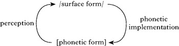
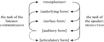
A formal account of a linguistic phenomenon has to start by stating the representations involved. For our purposes we need only two, namely the (abstract, discrete) phonological surface form and a (concrete, continuous) auditory-articulatory phonetic form. These two representations (see Fig. 2) are part of a more elaborate comprehensive model for bidirectional phonology and phonetics (Boersma Reference Boersma2007a), but any representations ‘above’ the surface form, such as the underlying form, are not discussed in this paper (except briefly in §§5.3 and 7.1), because they are not required for illustrating our point. Also, Fig. 2 keeps implicit any distinction between the auditory and articulatory parts of the phonetic form.
Processing models for phonetics and its interface with phonology.

The grammar model of Fig. 2 is bidirectional, i.e. it is used in two directions of processing: comprehension and production, as indicated by the arrows in the figure. In the comprehension direction, the (‘prelexical’) perception process maps an auditory-phonetic form to a phonological surface form; in the production direction, the phonetic implementation process maps a phonological surface structure to an auditory-articulatory phonetic form.
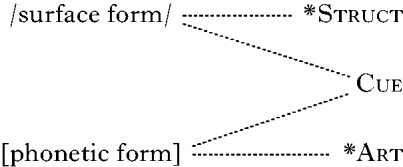
We formalise the relations between the representations in Fig. 2 with violable constraints, as in Fig. 3.
Grammar model for phonetics.
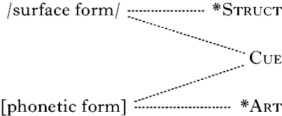
One of the reasons for modelling phonetics with constraints is that the output of the perception process tends to be restricted by the same structural constraints (*Struct in the figure) that have been proposed for phonological production. For instance, Polivanov (Reference Polivanov1931) proposes that Japanese learners of Russian perceive the Russian phonetic form [tak] as /.ta.ku./ because of a Japanese constraint on coda consonants, and the phonetic form [drama] as /.do.ra.ma./ because of a Japanese constraint against complex onsets.Footnote 5 Thus, the process that maps a phonetic form (or ‘overt form’ in the terms of Tesar & Smolensky Reference Tesar and Smolensky2000) to a phonological surface form is best regarded as being linguistic itself and therefore amenable to constraint-based modelling, a point previously made by Tesar (Reference Tesar, Hughes, Hughes and Greenhill1997), Boersma (Reference Boersma1998, Reference Boersma2007b), Tesar & Smolensky (Reference Tesar and Smolensky1998, Reference Tesar and Smolensky2000) and Pater (Reference Pater, Kager, Pater and Zonneveld2004).
We should point out here that modelling phonetic processing within a constraint-based framework such as OT does not imply that we regard low-level auditory and articulatory processing as belonging to a formal symbolic system specific to the human language faculty. On the contrary, a constraint-based decision mechanism like OT and/or Harmonic Grammar (HG; Smolensky & Legendre Reference Smolensky and Legendre2006) may well be typical of neural processing in general (Boersma Reference Boersma2003b: 444–445), and the success of OT in phonological theory may well be based on the fact that human phonological processing just uses this more general mechanism.
Having made plausible the claim that phonetic processing can be modelled with OT or HG, we can turn to the constraints proposed in Fig. 3. The relation between the phonological and the phonetic form is evaluated by cue constraints (Cue), and the phonetic form on its own is evaluated by articulatory constraints (*Art). As an example of a cue constraint, consider the fact that the duration of a vowel is a major cue to the voicing of a following obstruent in English, both in perception (Denes Reference Denes1955, Raphael Reference Raphael1972) and in production (Heffner Reference Heffner1937, House & Fairbanks Reference House and Fairbanks1953, Luce & Charles-Luce Reference Luce and Charles-Luce1985), but at most a weak cue in some other languages, both in perception (Morrison Reference Morrison2002, Broersma Reference Broersma2005)Footnote 6 and in production (Keating Reference Keating1979, Reference Keating and Fromkin1985). Hence, the cue constraint *[long vowel duration] /obs,−voice/ is ranked high in English but low elsewhere.
Because of the perception–production symmetry just noted we follow Boersma (Reference Boersma, Fanselow, Féry, Vogel and Schlesewsky2006, Reference Boersma2007a, Reference Boersmab) in assuming that the constraints in Fig. 3 are used bidirectionally. Bidirectionality in OT was previously proposed for faithfulness constraints by Smolensky (Reference Smolensky1996), for structural constraints by Tesar (Reference Tesar, Hughes, Hughes and Greenhill1997) and Tesar & Smolensky (Reference Tesar and Smolensky1998, Reference Tesar and Smolensky2000) and for cue constraints by Boersma (Reference Boersma1998, in a control-loop model that does not show dispersion).
For Fig. 3, bidirectionality works as follows. In perception, the choice between candidate surface forms involves structural and cue constraints. In this direction of processing, the cue constraints evaluate language-specific cue integration (Escudero & Boersma Reference Escudero and Boersma2004). For instance, the high ranking of *[long vowel duration] /obs,−voice/ in English predicts that an English listener, when confronted with an auditorily lengthened vowel, will be unlikely to perceive the following consonant as a voiceless obstruent, unless potentially conflicting constraints for other cues (or perhaps competing structural constraints) force her to. In phonetic implementation, the choice between candidate phonetic forms involves cue constraints and articulatory constraints. For instance, the high ranking of *[long vowel duration] /obs,−voice/ in English predicts that an English speaker, when intending to realise a voiceless obstruent, will be unlikely to lengthen the preceding vowel, unless articulatory constraints force her to.
We thus assume that speaker-listeners use cue constraints both in perception and in phonetic implementation, and that they rank (or weigh) these constraints identically in both directions of processing. The present paper shows that this bidirectional use of cue constraints leads to two asymmetries between perception and production, namely the prototype effect and the articulatory effect, and that languages that are stable over the generations have to cancel these two biases out against one another, thus striking an optimal balance between minimisation of articulatory effort and minimisation of perceptual confusion, without there being any goal-oriented dispersion mechanism in the whole system.
4 Sibilant inventories: dispersion of the spectral mean
The sounds with which we will exemplify the evolution of auditory contrast in this paper are the sibilants. We first make it plausible that sibilants indeed form a case of auditory dispersion.
The sibilants in a language can often be ordered along a one-dimensional acoustic continuum, namely the spectral centre of gravity or spectral mean (e.g. Forrest et al. Reference Forrest, Weismer, Milenkovic and Dougall1988, Gordon et al. Reference Gordon, Barthmaier and Sands2002), as in Fig. 4.Footnote 7 Articulatorily, the spectral mean correlates with frontness of the tongue and with frontness of the place of articulation.
Scale of spectral mean for eight sibilants.

The acoustic spectral mean corresponds monotonically to an auditory continuum: when listening to a continuously interpolated [ ] we hear something going up. This is not surprising: in the inner ear, as the sound [] is unfolding, the region of excitation is moving along the basilar membrane, from the centre towards the oval window. We therefore assume that the auditory continuum involved can be described as an auditory spectral mean expressed along the Erb scale (‘Equivalent Rectangular Bandwidth’; Moore & Glasberg Reference Moore and Glasberg1983), which in the region of the sibilants correlates approximately logarithmically with the acoustic frequency in Hertz; for instance, the auditory distance from 2000 to 4000 Hz approximately equals the auditory distance from 4000 to 8000 Hz (they are 5·7 and 5·2 Erb respectively). We pretend in this paper that the auditory spectral mean is the only relevant perceptual cue for sibilants. In reality, other cues for sibilant articulator and place include spectral peaks (e.g. Jongman et al. Reference Jongman, Wayland and Wong2000) and vowel transitions (e.g. Nowak Reference Nowak2006).
Sibilant inventories tend to be dispersed along the auditory spectral mean dimension, exhibiting all the effects mentioned in §2.1.
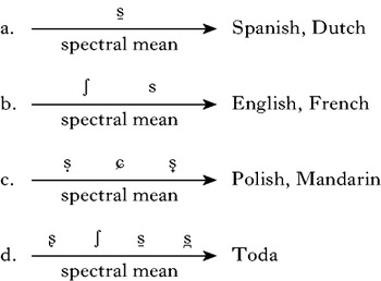
Languages with only one sibilant, such as Spanish or Dutch (if we disregard the marginal and unstable Dutch alveopalatal; but see note 15) usually employ a sound with a fairly central spectral mean (variously classified as /s/ or /ʃ/ by English listeners) such as the Dutch flat laminal alveolar [&sdbar;] (Mees & Collins Reference Mees and Collins1982: 6) or the Spanish concave retracted apical alveolar [&sdbar;] (Navarro Tomás Reference Navarro Tomás1932: 105–107, Harris Reference Harris1969: 192). This is illustrated in Fig. 5a. Note that a single symbol can be employed for two widely different articulations, a sign that sibilants can be identified by their sound rather than by their articulation. The single sibilant is never at an edge of the spectral mean scale; although Maddieson (Reference Maddieson1984: 423) lists the retroflex [ʂ] as the only sibilant in the Dravidian language Kota, Flemming (Reference Flemming2003: 354) convincingly illustrates that this is not the case: Kota [ʂ] is an allophone of the sibilant [s~ʧ] and occurs only adjacent to other retroflex sounds (Emeneau Reference Emeneau1944).
Dispersion of the spectral mean for inventories with one, two, three and four sibilants.

If a language has two sibilants, neither of them has a central spectral mean. Both sibilants are rather peripheral on the spectral mean dimension, as in English, which has a laminal, shallow-grooved and often rounded postalveolar [ʃ] and a deep-grooved alveolar [s] (Stone et al. Reference Stone, Faber, Raphael and Shawker1992: 260). Again, the articulations can vary markedly between languages (for English and French: Dart Reference Dart1991) and among speakers of the same language (Dart Reference Dart1991), which is often due to anatomical differences (Toda Reference Toda2005), but the auditory regions are similar.
In languages with a three-sibilant inventory, the three sibilant categories are equally spaced along the spectral mean dimension, usually implemented as (denti-)alveolar, alveopalatal and apical postalveolar, as in Polish (Puppel et al. Reference Puppel, Nawrocka-Fisiak and Krassowska1977) and Mandarin (Ladefoged & Wu Reference Ladefoged and Wu1984); for an overview of the various possibilities for the ‘apical postalveolar’ see Hamann (Reference Hamann2003). The sibilants produced by Polish women investigated by Zygis & Hamann (Reference Zygis and Hamann2003) have average acoustic spectral means of 3040, 4653 and 7439 Hz, which correspond to the evenly spaced auditory values of 24·40, 27·82 and 31·29 Erb. The three sibilants occupy a larger space than a two-sibilant inventory, illustrating the secondary dispersion effect (compare Fig. 5c with Fig. 5b). The Polish inventory is explicitly described in terms of auditory dispersion by Jones (Reference Jones2001), Padgett & Zygis (Reference Padgett and Zygis2003) and Zygis (Reference Zygis, Kosta, Błaszczak, Frasek, Geist and Zygis2003).
Finally, languages with four sibilants, such as Toda, occupy an even larger space along the dimension of spectral mean: at the low end, Toda has a subapical palatal sibilant [ʂ], which is the articulation with the lowest spectral mean of the attested sibilants. The descriptions for the other three Toda sibilants vary widely (Shalev et al. Reference Shalev, Ladefoged and Bhaskararao1993, Ladefoged & Maddieson Reference Ladefoged and Maddieson1996: 156–160, Ladefoged Reference Ladefoged2001: 153), so not much more can be said.
The observation that all of the dispersion effects of §2.1 seem to be attested in sibilant inventories suggests two things. The first suggestion is that the spectral mean continuum indeed represents the main auditory cue for sibilant place; this makes it plausible that modelling sibilants along a single auditory continuum, which we do in §§5 and 6, is a valid approach. Independent evidence for this is that some perception experiments have been able to model the [s]–[ʃ] continuum by shifting a broad spectral plateau of constant width (in log Hz) along the frequency scale (Repp Reference Repp1981). The second suggestion is that the articulatory-effort relations between the sibilants are similar to those of the auditory continua discussed in §2.1, i.e. that sibilants with central spectral mean values are easier to produce than those with peripheral values; this makes it plausible that including this articulatory-effort hypothesis in our modelling is a valid approach. Independent evidence for this comes from comparing the muscle activities required for producing central and peripheral sibilants. Sibilants with central spectral mean values like the Dutch flat laminal alveolar [&sdbar;] or the Spanish apical alveolar [&sdbar;] are produced by a simple raising of the articulators towards the roof of the mouth, without displacement or grooving of the tongue, and are thus as close as sibilants can get to the rest position of the tongue or to the average position of the tongue during vowels. At the high periphery of the spectrum, the deep-grooved alveolar sibilant (as in English) has a similar position to the Dutch non-grooved sibilant but requires additional activity of the upper fibres of the transverse tongue muscle (Hardcastle Reference Hardcastle1976: 96, 100–106, 134–137); at the low periphery of the spectrum we note that the apical palatal (retroflex) sibilant (as in Toda) has a similar tongue shape to the Spanish anterior sibilant but requires a larger movement of the tongue tip from a schwa-like position towards the palate and a stronger involvement of the upper longitudinal tongue muscle.
In summary, our knowledge of the spectral mean continuum and of the articulatory effort of sibilants is incomplete. This does not preclude the probability that the spectral mean continuum and articulatory effort really exist in human speakers and help shape sibilant inventories, as is strongly suggested by the cross-linguistic observations discussed in this section. We therefore assume both the continuum of the spectral mean and the hypothesis of peripheral articulatory effort. The fact that these hypotheses will make our model work can be regarded as further evidence in favour of them (if we may be allowed a little circularity).
In the following two sections, we show how the dispersion of sibilant inventories can be modelled without dispersion constraints. We illustrate this for English, a language with two sibilants, and for Polish, a language with three sibilants that show chain-shift effects, in §§5 and 6 respectively.
5 The English two-sibilant inventory
English has two sibilants, an alveolar /s/ and a postalveolar /ʃ/. In this section we first show how the English auditory environment leads us to predict the properties of an optimal English OT listener. We describe in detail how an English learner could come to be an optimal listener of her language, and perform a computer simulation showing that a virtual English learner arrives at a pronunciation that matches that of her environment. Having thus shown that in our simulations English is a stable language, we next show that a language with the exaggerated sibilant inventory /&sdsqrb;/–/ʂ/ is not stable but will instead turn into English within three generations. We do the same for the skewed and confusable inventory /&sdbar;/–/s/.
5.1 The English auditory language environment
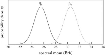
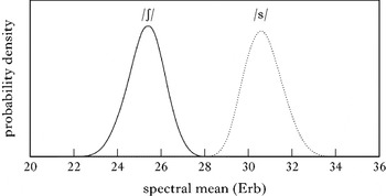
For simplicity we assume here that the auditory difference between the two English sibilants is wholly caused by a difference in their spectral means. The spectral mean of /s/, for example, will vary between speakers, vowel environments and acoustic and auditory conditions, as well as between replications by the same speaker. A listener will be able to normalise away some of this variation, but not all of it. Since the non-normalisable variation has multiple sources, the remaining distribution of spectral means for all the /s/ tokens that a listener hears is likely to have a bell-like shape, perhaps similar to the Gaussian shape in Fig. 6. We fix the average spectral mean of all normalised /s/ tokens in the listener's language environment at a slightly arbitrary value of 30·5 Erb (6656 Hz). Likewise, we assume for /ʃ/ a similar Gaussian distribution with an average spectral mean of 25·5 Erb (3478 Hz).Footnote 8 For both bell-shaped curves in Fig. 6 we choose a characteristic width (standard deviation) of 1·13 Erb.
Distributions for tokens of the English sibilants /ʃ/ and /s/ along the spectral mean.

The two distributions in Fig. 6, then, are the material that an adult listener has to work with, and that an infant learner has to make sense of. We assume somewhat arbitrarily that relevant spectral mean values for sibilants universally lie between 20·0 Erb (1789 Hz) and 36·0 Erb (16177 Hz).
5.2 The adult as an optimal listener
We explicitly assume that adult English listeners have learned to minimise the probability of misunderstanding, i.e. that they have become optimal listeners. To minimise the probability of misunderstanding, the optimal listener must show maximum-likelihood behaviour (Fisher Reference Fisher1922), i.e. she must classify an auditory event as the category that is most likely to have been intended by the speaker. For sibilants, the optimal English listener's decision criterion must be the frequency where the two curves in Fig. 6 intersect: she must perceive all tokens with a spectral mean below 28·0 Erb (4765 Hz) as /ʃ/, and all tokens above 28·0 Erb as /s/.
To model this correlation of spectral mean values and surface categories, we follow Escudero & Boersma (Reference Escudero and Boersma2004) in using a complete set of arbitrary cue constraints, which connect ‘all’ spectral mean values between 20·0 and 36·0 Erb to both sibilant categories. The constraints are summarised in (1).
(1)

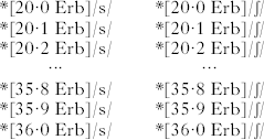
For perception, the constraint *[20·0 Erb]/s/ can be read as ‘an auditory spectral mean of [20·0 Erb] should not be perceived as the surface phonological category /s/’; for phonetic implementation, the constraint can be read as ‘a surface form /s/ should not be realised with a spectral mean of [20·0 Erb]’. For simplification, we discretise the spectral mean range into 161 steps of 0·1 Erb. Although the cochlea, the auditory nerve and the brain perform much more granular discretisations, a granularity of 0·1 Erb is fine enough to oversample any of the three local effects that we will discuss (see §§5.3 and 7.5 for arguments and proof that this discretisation is legitimate and consistent). Combining these 161 spectral mean values with the two sibilant categories results in a total of 322 cue constraints.
In connecting every possible spectral mean frequency between 20·0 Erb and 36·0 Erb to both sibilant categories, the cue constraints in (1) are very different from usual OT constraints, which either tend to express typological trends directly (e.g. markedness constraints) or tend to express universally preferred relations (e.g. faithfulness constraints). That is, the set in (1) has no preference for certain spectral mean values, for certain sibilants, or for connecting certain spectral mean values to certain sibilants, i.e. the constraints are not restricted to actually occurring spectral mean values or to actually occurring combinations of spectral means and sibilant categories. It is the ranking of these constraints that will have to be responsible for making the correct connections for English. From Fig. 6 we see, for example, that an optimal listener of English should perceive [26·6 Erb] as /ʃ/. A possible ranking that achieves this perception is given in the perception tableau in (2).
(2)

In tableau (2) we have given all possible candidates (only two, because we only consider the English sibilants), but we have restricted ourselves, for reasons of space, to only six of the 322 cue constraints. We can do this because 320 of our constraints have no preference for or against perceiving [26·6 Erb] as /s/ or /ʃ/. Tableau (2) illustrates that the correct classification of [26·6 Erb] relies solely on the ranking *[26·6]/s/≫*[26·6]/ʃ/. In the same way, we can establish rankings for the 160 remaining spectral mean values, e.g. *[31·4]/ʃ/≫*[31·4]/s/; the constraint *[28·0]/s/ will be ranked at approximately the same height as *[28·0]/ʃ/. We have now shown that the 322 constraints can be ranked in such a way that we can model an optimal listener for the distributions of Fig. 6.
However, such a language-specific ranking of 322 constraints is rather uninformative when it comes to predicting what kinds of sibilant-categorisation strategies are possible in the languages of the world. For one thing, the set of 322 constraints seems to generate an incorrect factorial typology: the traditional OT idea of factorial typology would predict the existence of languages with completely undispersed categories, and even the existence of categories with massively non-contiguous auditory correlates.Footnote 9 Such languages have not been shown to exist. Apparently, the idea of factorial typology must be incomplete, if cue constraints are to be the correct way to model perception. A general explanation for apparent gaps in the factorial typology is the idea that if UG allows grammars that are not attested in reality, then those grammars might be unlearnable or unstable over the generations (Boersma Reference Boersma2003b). We will therefore model both the acquisition and the evolution of these grammars, and show that undispersed and discontinuous categories are unstable over multiple generations of learners. The following subsection starts by illustrating how the acquisition of English sibilants is modelled with a simple learning procedure and algorithm.
5.3 Learning to become an optimal listener of English
We describe here the situation when a child already has correct lexical representations, but not yet an adult-like prelexical perception. That is, she already knows which lexical items have underlying |ʃ| and which have underlying |s|, but she does not know in the adult-like way of §5.2 what spectral mean values occur with which of the two surface sibilants.
During this acquisition period, the child will receive many tokens of /ʃ/ and /s/ drawn from the distributions in Fig. 6. Sometimes she will make a mistake, as in (3), which occurs when an adult speaker talking to the child pronounces an intended |ʃ| with a reasonable spectral mean of 26·6 Erb.
(3)

At this arbitrarily chosen point during her acquisition period, the child of tableau (3) happens to have the non-optimal ranking *[26·6]/ʃ/≫*[26·6]/s/ and therefore perceives the incoming auditory event [26·6 Erb] as the sibilant category /s/, as indicated by the pointing finger. However, the speaker had intended to transmit the lexical symbol |ʃ|, and the semantic and pragmatic context may lead the child's comprehension system to realise this (perhaps because the recognised lexical item was sheep). As a result, the child's lexicon can subsequently act as a ‘teacher’ or ‘supervisor’ and ‘tell’ her that she should have perceived /ʃ/ instead of /s/. This new knowledge by the child is indicated by the check mark in the tableau.
When a perception tableau such as (3) contains the child's own winning form (3a) as well as a form that she considers correct (3b), and the two forms are different, the child can conclude that she has made a mistake. As a result, she can take action by taking a ‘learning step’. A good strategy for executing a learning step is the Gradual Learning Algorithm (Boersma Reference Boersma1997, Boersma & Hayes Reference Boersma and Hayes2001), which is indicated by the arrows in the tableau: all constraints favouring the correct category are moved up, and all constraints favouring the child's own ‘incorrect’ winner are moved down.Footnote 10 As a result, the two cue constraints for the value [26·6 Erb] will be re-ranked slightly in the direction of the arrows. This process is called lexicon-driven perceptual learning (Boersma Reference Boersma1997, Escudero & Boersma Reference Escudero and Boersma2004).
The arrows in (3) represent small steps along a continuous scale of ranking. After having heard a number of [26·6 Erb] events that should have been perceived as /ʃ/, the learner will have swapped the rankings of *[26·6]/ʃ/ and *[26·6]/s/. From then on, the learner will perceive the auditory form [26·6 Erb] correctly as the category /ʃ/. The same successful learning applies to all other auditory forms for which one of the curves in Fig. 6 is close to zero, i.e. for all forms below approximately [26·7 Erb] or above approximately [29·3 Erb]. It now becomes clear why we called the Gradual Learning Algorithm a ‘good strategy’: the learner has become a maximum-likelihood listener for those auditory values. In the region where the curves in Fig. 6 overlap, something slightly different happens: the listener will necessarily continue to make some mistakes in prelexical perception, simply because e.g. an incoming token of [27·5 Erb] was intended as |ʃ| 75% of the time, but as |s| 25% of the time, as the curves show. In Stochastic Optimality Theory (Boersma Reference Boersma1997, Boersma & Hayes Reference Boersma and Hayes2001), where the ranking of every constraint is subject to a bit of additive noise at evaluation time, the listener is likely to vary her perceptual decisions. The Gradual Learning Algorithm then leads to a situation of probability matching: the learner will end up in an equilibrium situation in which she perceives [27·5 Erb] as /ʃ/ 75% of the time, but as /s/ 25% of the time. This works because the constraint *[27·5]/s/ will end up being ranked just above *[27·5]/ʃ/. This strategy of probability matching in perception, which is nearly as good as the maximum-likelihood strategy, has been shown to emerge automatically from the lexicon-driven learning mechanism both for one-dimensional continua (Boersma Reference Boersma1997) and for two-dimensional continua (Escudero & Boersma Reference Escudero, Boersma, Arunachalam, Kaiser and Williams2003).
There is one technical correction that has to be made. The above description of the learning algorithm involves changing the ranking of only one cue constraint, as if constraints did not influence their neighbours. A more realistic view of the auditory continuum has to take into account the fact that the properties of the basilar membrane in the inner ear are such that when a hair cell at a certain frequency is excited, several hair cells within a frequency distance of about 1 Erb will also be excited (Moore & Glasberg Reference Moore and Glasberg1983). This correlation between the firings of adjacent hair cells is reflected in the tonotopic map in the auditory cortex (Romani et al. Reference Romani, Williamson and Kaufman1982), and presumably in whatever neural device determines the auditory spectral mean. If we acknowledge this mutual correlation between adjacent spectral means and therefore assume a correlation between adjacent cue constraints, the learning algorithm must push bell-shaped dents into the shape of the cue-constraint curves. Following the simulations by Boersma (Reference Boersma1997: 51), we implement these dents as Gaussians with a standard deviation (an ‘effective resolution’) of 0·5 Erb. We have seen, for example, that the ranking of the constraint *[26·6 Erb]/s/ rises by 0·01 in (3). Our vicinity correction now implies that the constraints *[26·5 Erb]/s/ and *[26·7 Erb]/s/ will rise by 0·0098, the constraints *[26·4 Erb]/s/ and *[26·8 Erb]/s/ will rise by 0·0092, and so on; the constraints *[25·6 Erb]/s/ and *[27·6 Erb]/s/ will still rise by 0·01 exp (−0·5(1·0/0·5)2)=0·0014. The non-zero effective resolution guarantees a consistent discretisation of the spectral mean continuum by ensuring that the simulation results will be independent of the granularity as long as the spacing (which is 0·1 Erb in this paper) is at least several times smaller than this resolution (see §7.5).
In order to see exactly what happens in perception, and to be able to predict the effect of lexicon-driven perceptual learning on phonetic implementation, we cannot limit ourselves to the present description of the learning mechanism. Instead, we have to compute what listeners-speakers will do, and since any case involving more than two constraint curves is impossible to solve analytically, a computer simulation is the designated route.
5.4 Simulation of the acquisition of English perception
The learning of an English perception grammar can be simulated by computer. Our virtual learner has the 322 cue constraints in (1), and starts out having them all ranked at the same height of 100·0; as a result, the learner has an initial state where she perceives every incoming spectral mean value as /s/ 50% of the time and as /ʃ/ 50% of the time. At the same time we assume that this initial virtual learner already has correct lexical representations for all words with /s/ and /ʃ/. Although this combination of fully random prelexical perception and perfect lexical storage is obviously unrealistic, a more realistic modelling is very likely to exhibit effects that work in the same directions as the ones we will find here, although their size may differ (see §7.3 for discussion).
During the simulated acquisition period, our learner hears 1 million /ʃ/ and 1 million /s/ tokens in random order and with spectral mean values that are randomly drawn from the distributions in Fig. 6. Each token is also labelled as /s/ or /ʃ/ by the learner's lexicon. When hearing a token, the learner will perceive it into either category. In our simulations we set the standard deviation of Stochastic OT's evaluation noise (per tableau random variation in ranking) to a constant value of 2·0.
It can happen that the learner's perceived category is identical to the category the lexicon tells her she should have perceived. In such a case, the learner does not change her grammar. But if the perceived category is different from the one her lexicon says is correct, our learner changes the ranking of her cue constraints according to the scheme in tableau (3). The Gradual Learning Algorithm is here taken to have a constant plasticity (re-ranking step) of 0·01.
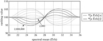
While listening to the 2 million tokens, our learner's cue constraints gradually move away from 100·0. The final perception grammar and three intermediate stages are shown in Fig. 7, where the constraints for the sibilant /ʃ/ are connected by a solid curve, and those for /s/ by a dotted curve. We can see, for instance, that for a spectral mean value of 24·0 Erb (2896 Hz), the dotted curve ends up having a ranking value of 105·0, and the solid curve one of 95·0. This means that the cue constraint *[24·0 Erb]/s/ ends up being ranked much higher than *[24·0 Erb]/ʃ/, and thus the token [24·0 Erb] is most often perceived as /ʃ/ in the final perception grammar (not always, because of the evaluation noise). In general, the lowest curve determines which category is perceived most often at any specific spectral mean value in Fig. 7.
A virtual learner acquiring the perception of the two sibilant categories of English: perception grammars after 2,000, 20,000, 200,000 and 2,000,000 input tokens.

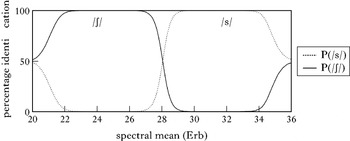
A complete OT analysis of a problem generally involves two parts, namely a description of the constraint ranking and a description of what outputs the grammar assigns to all of its inputs. While the ranking of all 322 constraints is given in Fig. 7, a description of the workings of the grammar would involve giving 161 input–output pairs, perhaps in the form of 161 perception tableaux that are analogous to tableau (2). And even these 161 tableaux would not suffice, because as a result of the evaluation noise of Stochastic OT it is fully possible that the same spectral mean value is sometimes perceived as /ʃ/, and sometimes as /s/. A full account of how the 161 spectral mean values are handled by the perception grammar therefore involves giving for each of the 161 spectral mean values the probability that it is perceived as /ʃ/ and the probability that it is perceived as /s/. An estimate of these is given in Fig. 8. This figure has been computed by running each of the 161 spectral mean values through the final perception grammar 100,000 times (with an evaluation noise of 2·0, as during learning), and noting how often the output was /ʃ/; dividing each of the 161 results by 100,000 yields an estimate of the probability that each spectral mean is classified as /ʃ/.Footnote 11 The probability of classifying it as /s/ is estimated in an analogous way.
Identification curves for the virtual listener of Fig. 7 (final state).

In Fig. 8 we see that the probability of perceiving /ʃ/ is greatest for those spectral values x for which the curve of *[x Erb]/ʃ/ lies furthest below the curve *[x Erb]/s/ in Fig. 7. This is a general property of Stochastic OT: the further constraint A is ranked above constraint B, the smaller the chance that B will overcome A at evaluation time.
Figure 8 confirms that the Gradual Learning Algorithm leads to optimal perception if the learner is given sufficient information. In the regions where she has heard a large number of spectral mean tokens (i.e. between approximately 23 and 33 Erb, as can be seen from inspecting Fig. 6), Fig. 8 shows that the learner has become an optimal (probability-matching) listener. For instance, the spectral mean of 27·5 Erb has (according to Fig. 8) a 75% probability of being perceived as /ʃ/ and a 25% chance of being perceived as /s/; hence, the odds of perceiving 27·5 Erb as /ʃ/ are three times as high as the odds of perceiving it as /s/; this ratio of 3 to 1 corresponds exactly to the relative heights of the two curves in Fig. 6 at [27·5 Erb].
However, the learner does not become optimal if she is given too little information. In the left periphery of the auditory space (around 21 Erb), the probability that such a spectral mean value was intended as /ʃ/ is very much higher than that it was intended as /s/, and this would predict that a probability-matching listener perceives such spectral mean values as /ʃ/ 100% of the time. Nevertheless, Fig. 8 shows that in this region the learner's perception grammar varies between perceiving /ʃ/ and /s/. This imperfection arises because the learner has not heard enough peripheral tokens to drag the two curves apart in this region.Footnote 12 The same holds for the right periphery of the auditory space (around 35 Erb).
It is interesting to see for which spectral mean values the probabilities are maximal. The probability-matching criterion would predict that the probabilities would be maximal in the regions near 20 and 36 Erb, but the scarcity of such tokens has moved the point of maximal separation quite far toward the centres of the two categories, i.e. towards 25·3 and 30·7 Erb. The spectral mean values for which the two curves are furthest apart are approximately 24·9 and 31·1 Erb. These locations can thus be said to represent the least confusable spectral mean tokens, and will turn out to be relevant when we consider how the listener of Fig. 7 will pronounce /ʃ/ and /s/ herself.
5.5 The near-optimal English listener's preferred production: the prototype effect
In a bidirectional model of phonetics, the cue constraints and rankings used by the listener in perception are also used in her phonetic implementation. When implementing an articulation, the cue constraint *[20·0 Erb]/s/ is read as ‘an /s/ should not be produced with a spectral mean of [20·0 Erb]’, and so on.
In (4) we see how the virtual learner of §5.4 would now produce an /s/, if only the cue constraints and rankings of Fig. 7 were involved.
(4)

The candidate [31·1 Erb] in (4) wins because the curve of the cue constraints for /s/ in Fig. 7 is lowest at this value (which is also where the two curves are maximally separated). If we compare this phonetic output to the token with the highest frequency in the distribution of Fig. 6, which has 30·7 Erb, we can see that our speaker produces an /s/ that has shifted slightly by 0·4 Erb from the /s/ that is most commonly produced by her surroundings.
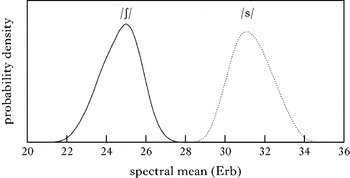
We now show that the shift is actually larger than the 0·4 Erb seen in (4). As a result of the evaluation noise of Stochastic OT, the winner in (4) will not always be 31·1 Erb. Instead, the winner will be the spectral mean value whose cue constraint (for /s/) happens to be lowest-ranked when evaluation noise is added to the ranking of each constraint. If we apply the same evaluation noise as in perception, namely with a standard deviation of 2·0, all spectral mean values with a ranking not much higher than that of *[31·1 Erb]/s/ are also likely to win. In Fig. 7 we see that the curve of *[x Erb]/s/ has a low plateau in the whole region between, say, 30·0 and 32·8 Erb, and these are all quite likely to win. The right-hand side of Fig. 9 shows the distribution of spectral values that we obtain by running the category /s/ 10 million times through production tableaux with the rankings of Fig. 7. The average spectral mean of the /ʃ/ category is 24·69 Erb, that of the /s/ category 31·35 Erb. The size of the shift (from the original 25·5 and 30·5 Erb) towards the periphery is therefore approximately 0·83 Erb.
Output distributions of the inverted perception grammar (distributions of ‘prototypes’).

What is behind this shift? From the discussion at the end of §5.4 we can infer that a probability-matching learning algorithm works in such a way that the constraints for values that are least likely to have been intended by the speaker as anything other than the dominant category in that region tend to be lowered furthest. Very roughly, the learning algorithm causes cue constraints to end up ranked lowest in auditory regions where the learner has heard the largest number of least confusable tokens. Teleologically speaking, our speaker prefers to produce an /s/ that is more peripheral than the average token that she has heard herself, because the auditory distance of such a token from the competing /ʃ/ is larger. What we observe here is the prototype effect in OT (Boersma Reference Boersma, Fanselow, Féry, Vogel and Schlesewsky2006). This phenomenon has been attested in experiments in the laboratory: when speakers of a language are asked to choose the best auditory instance of a sound category, they choose a more peripheral token than they would actually produce themselves (Johnson et al. Reference Johnson, Flemming and Wright1993), apparently because they choose the token that is least likely to present any other category than the one requested. It is important to note that although this explanation is couched in teleological terms (as if the listener-speaker knows about this), the underlying mechanism is not explicitly goal-oriented at all (and does not even know about auditory distance): the prototype effect occurs in OT simply because people employ in production the same cue constraint rankings that have optimised their prelexical perception.
The conclusion must be that learners will end up preferring more peripheral tokens than they have heard on average in their language environment. This would predict a sound shift if real learners really did that. But the phonetic implementation process of real speakers is not determined solely by their cue constraints. Articulatory considerations will be seen to keep the prototype effect within bounds.
5.6 Really speaking involves more constraints: the articulatory effect
Something is wrong with the assumption in §5.5 that phonetic implementation involves cue constraints alone. In real production the speaker is restricted by articulatory constraints as well. For instance, we can define the constraint *[31·2 Erb] as the articulatory constraint whose ranking reflects the articulatory effort associated with producing a spectral mean of 31·2 Erb. In the following we assume the independently plausible hypothesis (§§2.1, 4) that articulatory effort is minimal (though definitely not zero) for central auditory values of the spectral mean, and that more peripheral auditory values are harder to produce. If this hypothesis is correct (it at least explains the central tendency in single-sibilant inventories in §2.1), the articulatory constraints for peripheral auditory values must be ranked higher than those for more central auditory values.
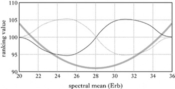
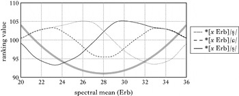
In the production of a sound, articulatory constraints interact with the cue constraints. This is illustrated with the production grammar in Fig. 10, where articulatory constraints are represented with a thick grey curve, following a parabolic shape reminiscent of effort curves found in biophysics (Hoyt & Taylor Reference Hoyt and Taylor1981). The cue constraints have the same rankings as in the perception grammar in Fig. 7, and are again represented as solid and dotted curves. Following Kirchner (Reference Kirchner1998), we assume for simplification that the ranking of articulatory constraints is fixed and not influenced by language-specific learning.Footnote 13
A production grammar for the two sibilant categories in English.

The interactions of articulatory and cue constraints in production become clear in the tableau in (5), where our learner tries to articulate /s/.
(5)

The candidate [31·1 Erb], which was the winner in the tableau without articulatory constraints in (4), no longer wins, because its articulation involves more effort than that of [30·7 Erb], which is the new winner. Loosely speaking, candidates below [30·7 Erb] are too indistinctive and candidates above [30·7 Erb] are too hard (note that in this tableau *[30·8 Erb] outranks *[30·7 Erb]/s/ despite the fact that in the region of 30·7 and 30·8 Erb the articulatory curve in Fig. 8 lies below the cue curve for /s/; there is no contradiction: in stochastic OT, constraints that are as closely ranked as these two will be ranked in the opposite order in a non-negligible fraction of the evaluations).
While the bidirectional use of cue constraints causes the categories to drift apart auditorily (§5.5), the presence of the articulatory constraints checks this expansion and drives the production distributions back towards the centre of the spectral mean continuum. Figure 11 shows the production distributions, estimated by running each sibilant category 10 million times through the grammar of Fig. 10 with an evaluation noise of 2·0.
The production distributions for the two sibilant categories in English.

The average spectral mean of the /ʃ/ category is 25·31 Erb, and that of the /s/ category is 30·70 Erb. When we compare this with the averages of Fig. 6 (25·5 and 30·5 Erb) and Fig. 9 (24·69 and 31·35 Erb), we conclude that the articulatory constraints have effectively prevented the categories from drifting apart auditorily: our English learner produces nearly the same average spectral means as her parents. Apparently, the articulatory effect has cancelled out the prototype effect. This balance of powers was first noted and modelled by Boersma (Reference Boersma, Fanselow, Féry, Vogel and Schlesewsky2006).
There is an important difference between the distributions in Fig. 6 and Fig. 11. In Fig. 6 the standard deviations of the two distributions are 1·13 Erb, and in Fig. 9 they are 1·03 and 1·06 Erb. In Fig. 11, however, the standard deviations are only 0·85 and 0·86 Erb: the distributions are narrower. Apparently, the articulatory effect has caused, in addition to the shift, an entrenchment of the produced distribution when compared with the distribution heard. This sharpening is an important property of our model, which will be seen to help to make the distributions stable over the generations (§5.7) and to allow the model to be compared favourably to other models (§7.4).
The near-exact cancelling of the articulatory and prototype effects is a direct result of our choice of parameters: knowing that English has a stable sibilant system, we chose the height of the articulatory curve to be the one in Fig. 10, not a higher or lower one. In this sense, the parameters of the model have been established on the basis of language data. Therefore we have to question the equal sizes of the prototype effect and the articulatory effect, and will do so in §§5.8 and 5.9. First, however, we show that the language simulated in §§5.4–5.6 is indeed stable over the generations.
5.7 Simulating sound change: a stable language
Are the average spectral means of the English sibilants, namely 25·5 and 30·5 Erb, indeed stable over the generations, or do they slowly drift? We test this by simulating the acquisition of the two sibilants over nine more generations.
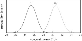
Some care has to be taken in how the produced spectral mean values of the first generations of learners are fed to the second generation. We cannot transmit the distribution of Fig. 11 directly from speaker to learner, because the only variation in the spectral mean values of Fig. 11 is due to decision noise in production. That is, the standard deviation of 0·85 Erb only reflects the evaluation noise in the production tableaux. The listener will be confronted with this source of variation (and not be able to normalise it away), but also with some non-normalisable between-speaker variation (because real learners will hear multiple speakers), some random variation within the speaker's muscle system (which is independent from the speaker's evaluation noise), the background noise in the air and the noise in the learner's ear. We represent these influences on the spectral mean together as transmission noise, with a standard deviation of 0·80 Erb. More precisely, the second generation of learners will be presented with spectral mean tokens computed from the grammar in Fig. 10, where to each token produced we add a value drawn randomly from a Gaussian curve with a mean of zero and a standard deviation of 0·80 Erb. The resulting distribution of spectral mean input values for generation 2 is given in Fig. 12, which was estimated by running each sibilant category 10 million times through the grammar of Fig. 10 with an evaluation noise of 2·0 and a transmission noise of 0·80 Erb. The standard deviations are approximately 1·17 Erb.
The sibilant environment of the second generation of learners.

Our second generation is thus represented by a learner who acquires a perception grammar in the way described in §5.4, on the basis of outputs of generation 1 modified by transmission noise (we again assume that the learner can distinguish the categories from each other). This learner then turns into a speaker by including articulatory constraints, as described in §5.6. We then feed tokens produced by this speaker, modified by 0·80 Erb transmission noise, to a new learner, our third generation. This learner acquires again a perception grammar and a production grammar; her transmitted output is used as input to the fourth learner, and so on.
In total we simulate this acquisition process for 10 learners in a row, with the simplifying assumption that every learner stands for a whole generation of speaker-listeners. Every learner receives 1 million /ʃ/ and 1 million /s/ tokens, and has a plasticity of 0·01 and an evaluation noise of 2·0.
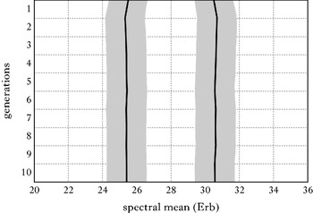
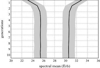
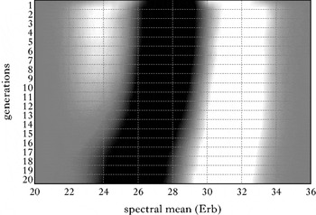
Over the generations, the English spectral mean values stabilise at about 25·40 and 30·60 Erb, and the standard deviations stabilise at about 1·18 Erb. This is shown in Fig. 13, where the black curves connect the single-speaker averages and the grey areas represent the standard deviations of distributions like those in Figs 6 and 12 (i.e. including transmission noise).
The spectral means of the two English sibilants and their stable learning over 10 generations.

Our simulated English (Fig. 6) turns out to be boringly constant (Fig. 13). There is no real change between the output of generation 1 and the output of generation 10 (except that the distributions are no longer Gaussian, but slightly skewed, as in Fig. 12). The next question is whether a language with different auditory distributions than Fig. 6 is equally stable, or whether it instead drifts away from its initial distributions.
5.8 Simulating sound change: a language with an exaggerated contrast is unstable
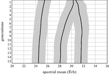
Here we simulate the learning of a language with a much more extreme two-sibilant contrast than English, i.e. [ʂ] vs. [&sdsqrb;], with spectral means of 23·0 and 33·0 Erb. Except for these initial distributions, everything else (including the shape and height of the articulatory constraint curve of Fig. 10) is the same in this simulation as in the one of §§5.4–5.7.
Figure 14 shows the result. For this ‘exaggerated English’, the second generation more or less learns the oversized range, although they reduce it to a much more moderate contrast of 24·83~31·18 Erb. Apparently, the articulatory effect outweighs the prototype effect for this generation; this comes as no surprise, since the articulatory curve in Fig. 10 (in the regions of 24·83 and 31·18 Erb) approaches the cue-constraint curve. The third generation has already shifted the system towards an unmarked articulatorily-perceptually balanced [ʃ] and [s]. Within two generations, the learners have changed the exaggerated English into plain English.
The development of the two sibilants in ‘exaggerated English’ over 10 generations.

The conclusion is that the articulatory and prototype effects can act independently, and work together to establish, non-teleologically, an optimal balance between articulatory ease and auditory contrast.
5.9 Simulating sound change: a language with a confusable contrast is unstable
If the optimal balance achieved in Figs 13 and 14 is characteristic of two-sibilant inventories in general, then the 25·4~30·6 Erb inventory should emerge for every possible initial inventory. The two cases that yet have to be investigated in this respect are the case of an initial ‘confusable’ English, where the categories are closely spaced, and the case of an initial ‘skewed’ English, where the categories are not positioned symmetrically around 28·0 Erb (as they are in Figs 13 and 14).
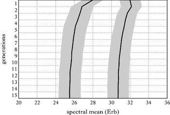
The two cases are combined in the simulation of Fig. 15, a language with initial sibilants at 28·0 and 32·0 Erb, which is both skewed (one sibilant has a central, the other a high spectral mean) and relatively confusable (the difference is only 4·0 Erb, rather than the 5·0 Erb of the earlier simulations).
The development of the two sibilants in ‘skewed and confusing English’ over 15 generations.

The first generation of learners moves the spectral mean values apart (to 26·8 and 32·2 Erb), immediately reaching an English-like distance of about 5 Erb. Apparently, the prototype effect plays a very fast role here; this confirms the repulsive dynamic nature of the present model and shows that the model will be able to handle phonetic enhancement and chain shifts. The articulatory effect is also seen to play a role, because the amount the lower category moves down (i.e. to the left in the figure) is larger than the amount the top category moves up. This effect works quite slowly, however: it takes quite a number of generations to obtain a perfectly symmetric inventory. The cause of the slowness is that the upper category ‘wants’ to move down but that this is hampered both by the repulsive force from the lower category and from the fact that the lower category itself experiences an upward bias from the articulatory effect. Nevertheless, a symmetric English-like inventory is eventually reached.
We can conclude from Figs 13–15 that our model predicts that, independently of the situation in generation 1, the inventory always evolves towards the same two auditory values. In other words, all stable languages with two sibilants are like English (or French, or German).
So we see that optimal dispersion indeed happens. Figs 13–15 all show the effect of the excluded centre (§2.1): the region around 28 Erb is avoided in languages with two sibilants. The next step is to look at other kinds of sibilant inventories: which of the dispersion effects will we see?
6 Larger, smaller and different inventories
In order to find all six dispersion effects discussed in §2.1, the present section discusses inventories with three and four categories (cf. Fig. 5). As special cases we also discuss an inventory with a single category and an inventory containing a non-contiguous category.
6.1 The Polish three-sibilant inventory: a chain shift
Polish used to have the sibilants /ʃ s&phosupj; s/ (Carlton Reference Carlton1991). If the dispersion principle is correct, and if the spectral mean is the only auditory cue that distinguishes these three sibilants, such an inventory cannot be stable. The simulation in Fig. 16 shows what happens if we start out with a language whose sibilants have spectral means of 25·5, 30·3 and 30·7 Erb (in order to make our point, we have taken values for /s&phosupj;/ and /s/ that are closer together than they probably actually were in medieval Polish).
The development of the three sibilants in Polish over 15 generations.

The first striking phenomenon that Fig. 16 shows is that the /s&phosupj;/~/s/ contrast is phonetically enhanced: the palatalised alveolar (the middle category) lowers its spectral mean beyond 29 Erb, i.e. into the [ɕ] region. This is reported to have happened in real Polish in the 13th century (Stieber Reference Stieber1952, Carlton Reference Carlton1991). The second thing that happens is that the laminal postalveolar (the sound on the left in Fig. 16) shifts down towards the apical postalveolar (‘retroflex’) [ṣ], which is reported to have happened in real Polish in the 16th century (Rospond Reference Rospond1971, though this sound is usually transcribed as postalveolar /ʃ/; see the discussion in Hamann Reference Hamann2004). Our simulation (when compared with the English simulations) confirms Jones' (Reference Jones2001) proposal that this second shift was caused by the first, i.e. that we are observing a contrast-enhancing push chain here: the /ʃ/ category is shifted down as a result of the approach by the lowering /ɕ/. Furthermore, we can observe the equally contrast-enhancing shift (again proposed by Jones Reference Jones2001) of the alveolar /s/ towards a more peripheral [&sdplus;], its present-day location (Puppel et al. Reference Puppel, Nawrocka-Fisiak and Krassowska1977). This simulation thus explains the present Polish sibilant system /ṣ ɕ &sdplus;/, which has spectral means very close to the 24·46, 28·08 and 31·59 Erb found here (the three female speakers recorded for the study by Zygis & Hamann Reference Zygis and Hamann2003 have average values of 24·40, 27·82 and 31·29 Erb). The grammar acquired by the fifteenth generation in Fig. 16 is given in Fig. 17; the articulatory constraint curve is the same as in Fig. 10. As before, this grammar is bidirectional. When given a certain spectral mean value, the grammar will most likely perceive it as the category for which the cue constraint at that spectral mean value is the lowest of the three. When given a category, the grammar will produce a spectral mean value where both the relevant cue constraint curve and the articulatory constraint curve are low; the average realised spectral mean values are 24·46, 28·08 and 31·59 Erb, as mentioned above. We have thus established an account of the Polish sibilant inventory without using dispersion constraints: only the cue and articulatory constraints of Fig. 17 are necessary (cf. Padgett & Zygis Reference Padgett and Zygis2003, who did use dispersion constraints for this example).
A production grammar for the three sibilant categories in Polish.

When we compare Fig. 16 to Fig. 15, we see all the dispersion effects discussed in §2.1. First, the centre category (around 28·0 Erb) is back in the picture. Second, the dispersion in Fig. 16 is even: both pairs of adjacent categories are removed from each other by approximately 3·6 Erb. Third, we see that the size of the auditory space is greater when there are three categories (7·1 Erb) than when there are two (5·2 Erb). Fourth, from the widths of the grey areas we see that the stable variation within a category is somewhat smaller when there are three categories (namely 1·12 Erb for the middle category and 1·15 Erb for the peripheral categories) than when there are two (1·18 Erb, according to §5.7). Fifth, we have observed a push chain when a lowering mid category caused the bottom category to lower as well. Sixth, we will observe a drag chain if we remove the bottom category from the final state in Fig. 16: from the simulation in §5.9 we know that the original mid category will move down to 25·4 Erb, allowing the top category to move down from 31·6 to 30·6 Erb. We conclude that we have faithfully modelled all aspects of auditory dispersion by assuming bidirectionality of cue constraints and a U-shaped articulatory effort curve, as in the production grammars in Figs 10 and 17.
6.2 A four-sibilant inventory
The largest inventory we consider is one with four sibilants, like Toda in Fig. 5. Independently of where the centres of the categories lie in the environment of the learners of the first generation, the centres of the categories evolve towards values around 24·4, 26·5, 29·5 and 31·6 Erb, i.e. the distances between the categories are again smaller than in the three-sibilant case, while the total space taken up has again increased (although very little). The spacing between the categories is somewhat greater in the middle than at the edges, probably because at the edges the limiting effect of the articulatory constraints is greater (this can be seen as a more precise formulation of §2.1.3). The final standard deviations are 1·13 Erb for the two outer categories and 1·22 Erb for the two inner categories, i.e. a bit larger than in the three-sibilant case.
We conclude that all dispersion effects identified in §2.1 remain valid in larger inventories (except the unexpectedly high within-category variation in the four-sibilant inventory, for which we have no explanation).
6.3 A one-sibilant inventory
The smallest inventory we consider is one with a single sibilant. The first generation of learners already turns up with a category centred at the centre of the auditory continuum, i.e. 28·0 Erb, and the standard deviation will be and stay a gigantic 3·03 Erb. The cause of this situation is that the learners do not learn: if the only category along the continuum is the unspecified sibilant /S/, they will perceive any spectral mean value as /S/, and therefore never make a mistake. As a result, all cue constraints stay ranked at 100·0, and in production the decision about which auditory value to pronounce is determined partly by which cue constraint happens to be lowest ranked, partly by the articulatory constraints.
The reader may object that the predicted one-shot shift to the centre is unrealistic, yet this is what we predict will happen in the absence of other phonological entities. In practice it will be very difficult to find such a situation: the single (retracted apico-alveolar) sibilant of Iberian Spanish, for instance, must cope with the existence of a rather strident /θ/ in the same language.
6.4 Can non-contiguous categories be learned?
The present model does not involve any representation of auditory distance. That is, the learner represents nothing more than 161 values along the spectral mean continuum, and does not necessarily know that they are ordered in a natural way. For instance, the virtual learner never needs to know that the spectral mean associated with the 37th value along the continuum (i.e. 23·6 Erb) lies in between those of the 27th value (22·6 Erb) and the 47th value (24·6 Erb). As a result, the constraint set of our virtual learner can easily represent an inventory where category 1 has spectral means around 26·5, 28·5 and 30·5 Erb, whereas category 2 has spectral means around 25·5, 27·5 and 29·5 Erb (as was mentioned in note 9). The question naturally arises, however, whether such discontiguous categories are not only representable, but learnable as well.
The answer turns out to be that discontiguous categories are ‘semi-learnable’: if the learner's environment contains a discontiguous category, then the learner's final category may still be discontiguous, but less so than the one in her environment, and within a number of generations the language will have changed into one with only contiguous categories.
An example is shown in Fig. 18. The initial inventory has a simple (monomodal) category (which we arbitrarily label /ʃ/) centred at 28·0 Erb with the usual relative frequency of occurrence of 50%, plus a bimodal category (which we label /s/) with a peak centred at 31·0 Erb with a relative frequency of 37·5% and a peak centred at 25·0 Erb with a relative frequency of 12·5%; all three peaks have a standard deviation of 1·13 Erb. Thus, both categories are equally likely, and the upper part of /s/ is three times more likely than the lower part.
The demise of a bimodally distributed category. Black=/ʃ/, white=/s/.

Figure 18 shows that the following generations continue to associate the /s/ category with two peaks. However, the lower peak shrinks slowly, and has almost disappeared after generation 11. After 20 generations, the English inventory has arisen again.
We conclude that in our model non-contiguous categories are learnable, but not stable over the generations. The ultimate cause of the development into monomodal distributions can be explained with Fig. 18 in the following way. The fact that the upper peak of /s/ is taller than the lower peak causes an asymmetry in the regions of confusion. That is, the region of confusion between the lower peak and /ʃ/ lies somewhat further from the centre of the continuum (namely around 26·0 Erb, which is 2·0 Erb away) than the region of confusion between the lower peak and /ʃ/ does (around 29·5 Erb, which is only 1·5 Erb away). As a result, /ʃ/ will shift down (i.e. to the left), which then pushes the lower peak of /s/ down into an articulatory more effortful region (push chain) and allows the upper peak of /s/ to come down into a less effortful region (drag chain). As a result, the articulatory bias against the lower peak of /s/ becomes greater than the articulatory bias against the upper peak, and this causes a slight preference in production for selecting tokens from the upper peak. This process is self-reinforcing, because it moves the boundaries between the three categories down.
We do not yet know how to assess our predicted relative learnability of bimodal distributions. If there exist mechanisms that cause such distributions to arise, we must be able to observe them in real languages, because such distributions are predicted to take ten generations to become monomodal. Whether actual languages do have this kind of transitory allophony in sibilants remains to be seen.Footnote 14
7 Discussion
Our simulations within a bidirectional model of phonetics realistically predict that a language with one, two, three or four sibilants automatically evolves towards a stable dispersed system, i.e. one that has single-peaked categories equally spaced along the auditory spectral mean continuum. The end result of such an evolution is independent of the spectral means of the categories in the first generation: given the number of categories, the resulting final categories will always be monomodal and have the same averages and standard deviations. Another thing our simulations have modelled realistically is the diachronic development of the sibilant inventory of Polish.
Our approach reconciles the standpoint of innocent misapprehension with that of auditory dispersion: speakers are not goal-oriented, but at the same time sound change tends to minimise perceptual confusion. Sound change at the level of the language learner is thus non-teleological, whereas at the abstract level of the observed language it is teleological. In this section we discuss the required assumptions and parameters of our model and compare them with those of earlier models.
7.1 General assumption 1: multiple levels of representation
If one wanted to express both phonetic and phonological considerations within OT's usual two-level unidirectional grammar model, one would have to mix detailed phonetic with discrete phonological representations (as in Flemming's 2002 OT version of Dispersion Theory). The reduction to non-teleological underlying mechanisms achieved in the present paper, by contrast, requires us to regard phonetic and phonological representations as separate and as equally important. This is accomplished by the model in Figs 2 and 3, in which the discrete phonological surface form and the detailed phonetic form are distinct representations connected by constraints in a way similar to how faithfulness constraints tend to connect the underlying form and the phonological surface form.
Proposing just one phonological surface form and one phonetic form does not suffice for a full-fledged model of phonology and phonetics. In order for the phonology to be able to handle alternations and metrical structure, we need at least an underlying phonological form as well. And if we want to distinguish more rigorously between the auditory and articulatory aspects of phonetics than we have done here, and if we want to distinguish between form and meaning in the lexicon (Apoussidou Reference Apoussidou2007: ch. 6), we arrive at the five-level OT (or HG) model in Fig. 19.
The bigger picture.

The arrows in Fig. 19 have been drawn in parallel to show that although the connections between the representations are local (e.g. cue constraints connect auditory to surface form and faithfulness constraints connect surface to underlying form, but there are no direct connections from auditory to underlying form), the optimisations are performed globally, i.e. by having constraints at different levels interact with each other. In our case of sibilant production, for instance, cue constraints (between auditory and surface form) have to be able to interact with articulatory constraints (at articulatory form); in other cases (Boersma Reference Boersma2007a, Reference Boersmab), cue constraints have been shown to interact with faithfulness constraints as well.
The full model of Fig. 19 thus rigorously separates the two discrete phonological representations from the two continuous phonetic representations, and is therefore compatible with many areas of current phonological investigation. At the same time, this model allows the phonology and phonetics to interact through global evaluation, thus reconciling the observation that phonological elements seem to be discrete with the observation that continuous-phonetic considerations seem to influence phonological behaviour.
7.2 General assumption 2: bidirectionality
Beside featuring multiple levels, the model has to be bidirectional, in the sense that the same constraints are used for modelling the speaker and the listener: the prototype effect arises because the constraint ranking that optimises the mapping from phonetic to surface form is reused in production (Boersma Reference Boersma, Fanselow, Féry, Vogel and Schlesewsky2006).
Within Optimality Theory, bidirectionality has been investigated in some depth by Blutner (Reference Blutner2000), Zeevat & Jäger (Reference Zeevat, Jäger, de Jongh, Nilsenová and Zeevat2002) and Jäger (Reference Jäger, Zeevat and Blutner2003). These proposals (for cases of competition in semantics and pragmatics) try to optimise the listener and the speaker at the same time. Jäger (Reference Jäger, Zeevat and Blutner2003) 's paper is very close to the present one in its general methodology of simulating acquisition and evolution and in its line of thought; for instance, Jäger presents several cases of language types that are both representable in UG and learnable, but unstable over the generations. However, Jäger's Bidirectional Gradual Learning Algorithm relies on a slightly teleological feature of evaluation in production: every candidate form in a production tableau has to be ‘hearer-optimal’, i.e. if taken as the input to a comprehension tableau (with the same rankings) it should be mapped to a meaning identical to the input of the production tableau.Footnote 15 This explicitly listener-oriented evaluation procedure thus militates against ambiguous (i.e. poorly ‘dispersed’) forms in production, and Jäger relies on it for establishing the diachronic emergence of pragmatic case marking (which enhances the semantic contrast between subject and object). It would be interesting to investigate whether our arguably simpler procedure (optimise comprehension only, then just speak) would be able to handle the complex cases that Jäger discusses.
Outside OT, bidirectionality has been proposed for an exemplar model of phonology. In exemplar theory (Johnson Reference Johnson, Johnson and Mullennix1997, Lacerda Reference Lacerda1997), the listener stores in her memory the actual phonetically detailed tokens (‘exemplars’) she hears, together with their category labels. Pierrehumbert (Reference Pierrehumbert, Bybee and Hopper2001) proposes that the listener will subsequently use the same exemplars in production. It has been claimed by both Lacerda (Reference Lacerda1997: 27) and Pierrehumbert (Reference Pierrehumbert, Bybee and Hopper2001: 143) that a prototype effect similar to the one we derived in §5.5 will arise in listener's goodness ratings (although neither Lacerda nor Pierrehumbert provides the simulations to prove this).Footnote 16 Blevins (Reference Blevins2004: 285–289) proposes that the shifted ‘prototypes’ (i.e. the ‘best’ exemplars in goodness ratings) will be used in production as well (2004: 288), ultimately leading to chain shifts. That this is indeed possible in exemplar theory was proven by the simulations by Wedel (Reference Wedel2004: 140–169, Reference Wedel2006: 261–269), which use a device for detecting ambiguous tokens, i.e. tokens whose auditory values lie in the regions of overlap between two categories. By refusing to store the ambiguous tokens as exemplars at all, or by allowing them to be stored in the incorrectly perceived category (rather than in the category intended by the speaker, as happens e.g. in our lexical supervision), Wedel derives the required repulsion of categories.Footnote 17 The similarity between Wedel's simulations and ours is that the prototype effect is caused by avoiding regions of overlap (because cue constraints don't move apart in those regions, or because exemplar storage fails in those regions). The difference is that in our model the prototype effect is intrinsic to the bidirectional use of constraints, so that this model, in contrast to Wedel's, makes the empirical prediction that dispersion-like effects must appear in all areas of the grammar, not just in the ‘phonetics’. In §8 we speculate on possible applications.
All in all, our model seems to be the one in which the prototype effect in perception and its repulsive effect in production come about most directly and forcefully. Given bidirectional OT with optimisation of comprehension, we would in fact need complex additional machinery if we did not want categories to repel each other. The fact that this simplest possible bidirectional OT model already exhibits this effect, an effect that arguably contributes to the success of the species that have it, suggests the idea that biological evolution may well have selected bidirectional constraint competition as a general decision-making mechanism, especially if similar phenomena will turn out to occur in other parts of the grammar (see again §8).
7.3 Assumptions required to go beyond the limitations of the present paper
Our present simple implementation of the model comes with several limitations.
Consider the problem mentioned in §5.4 that it is unrealistic to assume an initial state with fully random prelexical perception together with perfect lexical representations. In a more realistic simulation we will have to take into account the likely fact that the contrast between the categories /s/ and /ʃ/, which has to have been acquired before these categories can be used in lexical entries, has emerged in the learner as the result of prior distributional learning, which should have given a non-trivial initial ranking of the cue constraints. An explicit proposal was provided by Boersma et al. (Reference Boersma, Escudero and Hayes2003). We will also have to take into account the likely fact that lexical representations are acquired in concurrence with prelexical perception. An explicit proposal was provided by Apoussidou (Reference Apoussidou2007). Both refinements will require a comprehensive simulation that is far outside the scope of the present paper.
Another limitation is that our model makes no explicit provisions for diachronic merger. This is because we assumed that even if two categories were very close to each other, as in the initial situation of Fig. 16, the learner was given correct labels by her lexicon. However, a beginning learner does not know beforehand how many sibilants her future language has, and therefore at least has to rely on a stage of distributional learning, in which she establishes the number of categories: if the distributions of two adjacent adult categories overlap too much, these distributions may not form separate peaks and the infant may posit a single category instead of two (e.g. Boersma et al. Reference Boersma, Escudero and Hayes2003); if she does, a merger has occurred. The comprehensive simulation mentioned in the previous paragraph will take care of this situation. Thus, the present model, combined with the independently needed earlier stage of category creation, accounts for both chain shift and merger.
In the present paper we have limited ourselves to a case with a single auditory dimension. Boersma (Reference Boersma2007c) applies the present model to a case with two auditory continua, namely the simulation of an inventory with five vowels within a vowel space that has two auditory dimensions: height (first formant) and backness (second formant). The number of cue constraints scales linearly with the number of continua: if we divide the height and the backness continuum into 100 points each, we require 200 cue constraints per vowel (Boersma & Escudero Reference Boersma and Escudero2008). Boersma's (Reference Boersma2007c) simulations yield the expected dispersion effects for vowels. It is imaginable that for cases with many auditory dimensions, the simulations might interestingly end up in locally optimal inventories, rather than in the globally optimally dispersed inventories found in the present paper; in fact, globally optimal inventories can be defined in Harmonic Grammar and in Maximum Entropy grammars, but not in OT, as simulations involving eternal optimisation by Boersma (Reference Boersma2003a) have shown.
Finally, we have limited our discussions to fixed locations of category centres, rather than acknowledging the fact that speakers adapt their auditory spaces to pragmatic circumstances on the fly. Such facts could be included in a way analogous to Boersma's (Reference Boersma1998: 208–215) modelling of the dependence of auditory forms on stress and context. Under circumstances of extra articulatory effort (e.g. fast speech), for instance, speakers could indiscriminately raise the rankings of all articulatory constraints by the same amount (Boersma Reference Boersma1998: 275). The auditory values will then become less dispersed immediately (i.e. without learning), just as in the real world. Under circumstances of extra clarity (e.g. addressing a crowd), speakers could raise the rankings of all cue constraints, as well as perhaps those of all faithfulness constraints (Boersma Reference Boersma1998: 275), sensorimotor constraints and lexical constraints. The auditory values are then predicted to become more peripheral immediately (i.e. without learning), just as in the real world. In other words, our model could account for instant adjustments in hyper- and hypospeech (Lindblom Reference Lindblom, Hardcastle and Marchal1990a) with an intricacy familiar from the multitude of more discrete constraint-ranking proposals in the OT literature.
7.4 Assumed devices
Beside the general assumptions of multiple representations and bidirectionality mentioned in §§7.1 and 7.2, our model may require some devices more specific to auditory dispersion. In this section we mention these assumptions and compare them with those of the main non-OT account (exemplar theory; see §2.2) and the main previous OT accounts (Flemming, Padgett and Sanders; see §2.3).
Our first assumption is that of the existence of transmission noise. We think that this is not controversial, and would be included in any explicit model of language transfer. The transmission noise is not represented in the mind or brain of the speaker-listener, but comes for ‘free’ in the transmission between the speaker's production decision and the listener's auditory-phonetic input.
Our second assumption is that of the greater articulatory effort associated with peripheral auditory values. This assumption also appears explicitly in Flemming (1995: 46), and would probably be required in Wedel's (Reference Wedel2004, Reference Wedel2006) exemplar-based dispersion model if it wanted to account for central tendencies.
Our next assumption involves the way in which the auditory information associated with a category is stored in the brain. One could store this information in a small number of parameters, such as the basic statistics (average and standard distribution) of the spectral mean distribution, or with the help of category boundaries, or as a prototype; OT dispersion theory, for instance, seems to require a storage in terms of prototypes, because categories are expressed with auditory values such as ‘low F2’. In the present model, none of these parameters is represented, although they could be computed from identification curves such as Fig. 8, distributions such as Fig. 11 or tableaux such as (4). We know of no proposals in the literature that are based on stored statistics, boundaries or prototypes and that come with a learning procedure that exhibits dispersion effects. Another problem with representing such parameters would be that in a full model they would have to be additional representations, appearing in between a granular auditory representation, such as the one coming in from the auditory nerve, and the phonological surface level at which the categories are represented; in the present model, the cue constraints are the direct connections between the auditory and the phonological level.
An alternative way of storing the auditory information is by using episodic memory. Exemplar theory requires the listener to store every category as a set of multiple exemplars, each of which records all auditory values associated with a specific auditory event that the listener has heard; our model does not need to store exemplars, because the frequency effects that exemplar theory ascribes to the multiplicity of exemplars tend to derive automatically from the rankings of the many constraints. The most costly method of storing the auditory information would be in terms of joint distributions of auditory values. For instance, the vowel space discussed in §7.3 would require 10,000 points to maintain a joint distribution for the two continua; in other words, models that store distributions directly scale poorly (i.e. exponentially) with the number of dimensions. In our model, the distributions are only very indirectly represented in the rankings of the cue constraints, and the model scales well (i.e. linearly) with the number of dimensions (§7.3). We cannot yet assess how the exemplar models of Lacerda (Reference Lacerda1997) and Pierrehumbert (Reference Pierrehumbert, Bybee and Hopper2001) scale with increasing dimensionality, because they only address single continua.
For the stability of the standard deviation of a category over the generations, our model has to assume nothing: the stability is an automatic consequence of the balance between the entrenchment effect of the articulatory constraints (§5.6) and the transmission noise. By contrast, exemplar theory has to invoke special measures to keep the standard deviation stable, as noted by Pierrehumbert (Reference Pierrehumbert, Bybee and Hopper2001: 149–152): if speakers just randomly choose from among their previously stored exemplars, the transmission noise will soon increase the variation between the exemplars of the category; as a consequence, Pierrehumbert has to propose that speakers use an average of multiple exemplars, and this leads to the required entrenchment. Wedel (Reference Wedel2006) calls this averaging ‘within-category blending inheritance’; the present model, by contrast, can get by with choosing a single existing auditory value.
Our model does not have to represent or compute auditory distance. In most exemplar models, listeners need auditory distances to compute the degree to which an existing exemplar is activated (Nosofsky Reference Nosofsky1988: 701, Kruschke Reference Kruschke1992: 23, Johnson Reference Johnson, Johnson and Mullennix1997: 147, Pierrehumbert Reference Pierrehumbert, Bybee and Hopper2001: 141; an exception is Lacerda Reference Lacerda1997), and when production is included in the model, speakers need auditory distance to compute the contribution of various exemplars in establishing the ‘entrenchment’ that has to undo the effects of the transmission noise (Pierrehumbert Reference Pierrehumbert, Bybee and Hopper2001: 149). A very far-reaching representation of auditory distance is needed in OT Dispersion Theory (Flemming Reference Flemming1995) to assess violations of MinDist. For instance, a language user with categories (or rather, category prototypes) A, B and C has to compute all distances A–B, B–C and A–C, and subsequently to decide which of these is the smallest. In all these models, the computation of auditory distance is regarded as a phenomenon that comes for free; to complete these models, however, an explicit account would have to be given of the underlying mechanism that computes such auditory distances, which seems to require a non-trivial future extension to these models. In our model, by contrast, auditory distance does not have to be computed directly at any point, nor is it represented explicitly at any point; auditory distance effects do arise (as in the identification curves of Fig. 8), but they emerge indirectly from the underlying mechanism of acquired constraint ranking, which reflects auditory confusability more directly than auditory distance (see note 13 for some empirical support). In our model, a possible unwanted side effect of not representing auditory distance, namely the learnability of the non-existent or very rare non-contiguous categories, is counteracted by the inherent instability of such categories over the generations (§6.4).Footnote 18
Finally, the present model does not represent any devices explicitly oriented to the goal of improving dispersion, such as the dispersion constraints MinDist (Flemming Reference Flemming1995), Space (Padgett Reference Padgett2003a, Reference Padgettb) or  n-P (Sanders Reference Sanders2003). Whether this means that dispersion constraints are superfluous for phonological theory depends on the question of whether they can be used for other things beside evaluating inventories. For instance, dispersion constraints have been used to describe diachronic phonetic enhancement (Sanders Reference Sanders2003: 123). Since phonetic enhancement is also a feature of our model (§§5.9, 6.1), dispersion constraints do not seem to be required for modelling such phenomena. An opposing use of MinDist has been to describe neutralisation effects: because of the way MinDist has been formulated (loosely ‘small auditory distances between contrasting categories are not allowed’), one way to satisfy it is to neutralise the contrast completely. One such effect, namely unconditional diachronic merger, is handled in our model by the innocent misapprehension that takes place in the infant's distributional learning stage (§7.3). The other effect, namely conditional merger, involves the phonologically more interesting cases of assimilation and positional neutralisation (e.g. Flemming 1995: 119–151). The bidirectional phonology and phonetics model generally accounts for such phenomena by ranking cue constraints over faithfulness constraints (Boersma Reference Boersma2007a: 2035).Footnote 19 A rigorous analysis in these terms of all effects ascribed to dispersion constraints in the literature falls outside the scope of the present paper.
7.5 Sensitivity to the parameter settings
The present model requires six parameters: the shape and height of the fixed articulatory effort curve (Figs 10 and 17), the amount of transmission noise (0·8 Erb), the plasticity (0·01), the number of training data (1 million per category), the granularity of the spectral mean continuum (0·1 Erb) and the effective resolution (0·5 Erb).
The results are not qualitatively sensitive to the exact values of these parameters. Raising the effort curve or making it steeper toward the sides will move the emerging category centres further towards each other, whereas raising the transmission noise will move them further apart. Raising the plasticity by a factor of 10 moves the curves of the cue constraints slightly further apart, although this effect can be compensated by reducing the number of training data by a factor of 10. Even reducing the number of training data by 99%, i.e. to 20,000 (thus stopping after the second step in Fig. 7), gives very similar results to those found in the reported simulations: the only difference is that the category centres will turn up somewhat closer together (e.g. by 15% for English). Raising the granularity of the spectral mean continuum by a factor of 10, so that the spacing is 0·01 Erb, does not change any results at all: the results will be identical to the ones reported as long as the spacing is several times smaller than the transmission noise and the effective resolution; this proves that the Gaussian dent method of §5.3 is a correct way to turn a continuum into a set of discrete points. Finally, reducing the effective resolution from 0·5 Erb to zero, effectively making the constraints insensitive to their neighbours, causes fewer tokens to appear in each spectral mean value, hence a reduction of the distance by which the cue constraints will move; but the overall phenomena (prototype effect, entrenchment, stability) do not qualitatively change.
7.6 Dependence on the specific framework of constraint interaction
Our model does not depend on the particular framework in which one models constraint interaction. Although our simulations in §§5 and 6 were done in Stochastic OT, they can equally well be done with Noisy HG (Boersma & Escudero Reference Boersma and Escudero2008), which is Harmonic Grammar (Smolensky & Legendre Reference Smolensky and Legendre2006) with additive evaluation noise, or with Maximum Entropy models (Goldwater & Johnson Reference Goldwater, Johnson, Spenader, Eriksson and Dahl2003). For the simple one-dimensional learning cases in §5.3, Noisy HG is identical to Stochastic OT, and the learning algorithm for Noisy HG (Boersma & Escudero Reference Boersma and Escudero2008) is identical to the Gradual Learning Algorithm for Stochastic OT (the algorithm for Noisy HG is generally identical to Soderstrom et al.'s Reference Soderstrom, Mathis and Smolensky2006 learning algorithm for non-noisy HG). For our case, the difference between Stochastic OT and Noisy HG therefore lies not in perception, but only in production. In Noisy HG, the height of the articulatory effort curve has no influence on the result; only its shape counts: with the shape of Fig. 10, two-category learners will end up with category centres of 25·6 and 30·4 Erb. For Maximum Entropy grammars, which have a different way of determining winning candidates, tableau (3) still holds: the learning algorithm (Jäger Reference Jäger, Zaenen, Simpson, King, Grimshaw, Maling and Manning2007) is generally identical to that of HG and Noisy HG. In Maximum Entropy, the shape of the acquired perception grammar is similar, though not identical, to Fig. 7; however, no entrenchment effect is produced, so that a succession of two-category learners will ultimately end up smoothing out the two categories; a stable situation is reached only if the transmission noise is unrealistically set to zero. We conclude that with all three constraint-based frameworks, the prototype effect is in full operation, but only Stochastic OT and Noisy HG exhibit the equally required entrenchment effect.
7.7 Are phonological features innate or emergent?
In this paper we have used /ʃ/ and /s/ as arbitrary labels that had no preference for any specific positions along the spectral mean continuum. Given this arbitrariness, our model seems slightly more compatible with the viewpoint that phonological features themselves are emergent (Boersma Reference Boersma1998, Blevins Reference Blevins2004, Mielke Reference Mielke2004) than with the viewpoint that phonological features are innate. This is because innate features just seem to be in the way of our learning procedures. For instance, if distributional learning creates three peaks, and therefore three categories, along an auditory continuum, it is easier to give these categories arbitrary labels than to associate them to innate feature values, a procedure that would require an additional mapping device. We realise, though, that the controversial issue of innateness vs. emergence is too big for the present paper.
8 Conclusion: the innocent emergence of optimal dispersion
The two assumptions of multiple levels and bidirectionality have explained the origins and stability of auditory dispersion over the generations. It has turned out that if the auditory category centres are too wide apart, the learner's articulatory effect will be greater than her prototype effect, forcing her to shift her production partly towards a smaller, more naturally dispersed inventory, and that if the auditory category centres are too close, the learner's articulatory effect will be smaller than her prototype effect, forcing her to shift her production towards a larger, again more naturally dispersed inventory. Over the generations, every language innocently evolves towards a stable, typologically natural inventory that strikes an optimal balance between articulatory ease and auditory contrast. Everything else being equal, we expect a stable language with two or three sibilants to have the same auditory inventory as English or Polish. In reality, of course, the inventory will be influenced by the rest of the phonological system of the language, because tout se tient.
Our findings are relevant for constraint-based phonological theory, because they show that dispersion effects emerge automatically and non-teleologically in the phonology–phonetics interface, and that therefore phonological theory does not have to take them into account at higher levels such as in the phonological surface form (by dispersion constraints) or in the relation between underlying and surface form (by faithfulness constraints).
By deriving dispersion directly from independently needed cue constraints and the independently defended idea of bidirectionality, the results provide support for the idea that humans use constraint ranking or weighting as a decision mechanism (but no support for more linguistically specific concepts of OT such as factorial typology, innate constraints or richness of the base). We have noted that dispersion can be achieved in exemplar theory as well, namely by extending its basic idea with blending inheritance (Pierrehumbert Reference Pierrehumbert, Bybee and Hopper2001) and lexical decision failures (Wedel Reference Wedel2004, Reference Wedel2006). Both frameworks are a priori plausible, because both have their roots in explicit models of the brain: exemplar theory in models of episodic memory, and OT/HG in connectionist models. The empirical difference between the two frameworks as regards dispersion is that the constraint-based model predicts that dispersion effects pervade every level of processing where connecting constraints are used bidirectionally: the bidirectional use of faithfulness constraints (between surface and underlying form in Fig. 19) yields homophony avoidance, the bidirectional use of lexical constraints (between underlying form and morpheme in Fig. 19) yields homonymy avoidance; even in OT semantics, bidirectionality of constraints is predicted to lead to listener-oriented effects in production. By contrast, current exemplar models do not predict such effects, unless more extensions are added. In the end, whether the correct model of human language processing will be similar to a constraint-based model or to an exemplar-based model, or to a synthesis of the two, will depend on future research on overt human behaviour (linguistics and psycholinguistics) as well as on future research on the underlying mechanism (the brain).
 ] and any more fortis varieties. For most languages the sources do not make a principled distinction.