2 Modified Hasegawa–Wakatani model

Hasegawa–Wakatani model (HWM) describes the dynamics of the fluctuations of the electrostatic potential $\unicode[STIX]{x1D711}$ and the electron density $n$ in the $x{-}y$ plane perpendicular to the magnetic field (Hasegawa & Wakatani Reference Hasegawa and Wakatani1983). The equilibrium density gradient is held fixed in the HWM. One of the two equations in the model enforces the steady current and the other is the electron continuity. The electric current flows in the direction perpendicular to the magnetic field due to the ion polarization drifts and in the parallel direction due to the resistive motion of the electron fluid. The electron resistive current is proportional to the sum of the electric force and the density gradient with the coefficient being the conductivity $\unicode[STIX]{x1D70E}$. Typical units of the HWM are $\unicode[STIX]{x1D70C}_{s}$ for the spatial scale, $L_{n}/c_{s}$ for the time, $(T_{e}\unicode[STIX]{x1D70C}_{s}/eL_{n})$ and $(n_{0}\unicode[STIX]{x1D70C}_{s}/L_{n})$ for $\unicode[STIX]{x1D711}$ and $n$, respectively, where $L_{n}$ is the length scale of the equilibrium density, $c_{s}=\sqrt{T_{e}/M_{i}}$ and $\unicode[STIX]{x1D70C}_{s}=c_{s}/\unicode[STIX]{x1D6FA}_{i}$. The electron temperature is $T_{e}$, the electron charge $e$, the ion mass $M_{i}$, the ion gyro-frequency $\unicode[STIX]{x1D6FA}_{i}$ and the background density $n_{0}$.

The modified version of the HWM (mHWM) excludes the resistive damping of the zonal mode which changes only along the direction of the background density gradient (Numata, Ball & Dewar Reference Numata, Ball and Dewar2007). In dimensionless form the mHWM is

(2.1)$$\begin{eqnarray}\displaystyle & \displaystyle \unicode[STIX]{x2202}_{t}\unicode[STIX]{x1D714}+[\unicode[STIX]{x1D711},\unicode[STIX]{x1D714}]=\unicode[STIX]{x1D6FC}(\tilde{\unicode[STIX]{x1D711}}-{\tilde{n}})-\unicode[STIX]{x1D708}\unicode[STIX]{x1D6FB}_{\bot }^{4}\unicode[STIX]{x1D714}, & \displaystyle\end{eqnarray}$$

(2.2)$$\begin{eqnarray}\displaystyle & \displaystyle \unicode[STIX]{x2202}_{t}n+[\unicode[STIX]{x1D711},n]=-\unicode[STIX]{x2202}_{y}\unicode[STIX]{x1D711}+\unicode[STIX]{x1D6FC}(\tilde{\unicode[STIX]{x1D711}}-{\tilde{n}})-\unicode[STIX]{x1D708}\unicode[STIX]{x1D6FB}_{\bot }^{4}n, & \displaystyle\end{eqnarray}$$

where $\unicode[STIX]{x1D714}=\unicode[STIX]{x1D6FB}_{\bot }^{2}\unicode[STIX]{x1D711}$ is the vorticity, $\tilde{\unicode[STIX]{x1D711}}=\unicode[STIX]{x1D711}-\bar{\unicode[STIX]{x1D711}}$ and ${\tilde{n}}=n-\bar{n}$ are the non-zonal parts. The zonal components $\bar{\unicode[STIX]{x1D711}}$ and $\bar{n}$ are independent of $y$ because they are the averages of the corresponding fluctuations over $y$. With the units, the gradient of the equilibrium density $n_{0}$ is fixed to be $\unicode[STIX]{x1D6FB}n_{0}=-\hat{\boldsymbol{x}}$. On the left-hand sides of (2.1) and (2.2) the Poisson brackets, e.g. $[\unicode[STIX]{x1D711},\unicode[STIX]{x1D714}]=(\hat{\boldsymbol{z}}\times \unicode[STIX]{x1D735}_{\bot }\unicode[STIX]{x1D711})\boldsymbol{\cdot }\unicode[STIX]{x1D735}\unicode[STIX]{x1D714}$, denote the $\boldsymbol{E}\times \boldsymbol{B}$ advection. The electron diamagnetic drift is along $y$, and the magnetic field is along $z$. The terms $\unicode[STIX]{x1D6FC}(\tilde{\unicode[STIX]{x1D711}}-{\tilde{n}})$ in (2.1) and (2.2) come from the divergence of the parallel resistive current and the parallel compression, respectively. Variation along the magnetic-field direction is parametrized by $\unicode[STIX]{x1D6FC}$ that is proportional to $\unicode[STIX]{x1D70E}$ and inversely proportional to the square of a typical length scale along $z$. Since $\unicode[STIX]{x1D70E}$ increases with the electron temperature $T_{e}$, the parameter $\unicode[STIX]{x1D6FC}$ is roughly larger for higher $T_{e}$. Electrons are almost adiabatic if $\unicode[STIX]{x1D6FC}>1$. Artificial hyper-diffusion of order four is introduced in order to cut off the smaller-scale non-zonal fluctuations with the coefficient $\unicode[STIX]{x1D708}$. For the zonal fields artificial diffusion of order 2 with different coefficient $\bar{\unicode[STIX]{x1D708}}$ is used.

Evolution of the non-zonal fields is reduced from (2.1) and (2.2)

(2.3)$$\begin{eqnarray}\displaystyle & \displaystyle (\unicode[STIX]{x2202}_{t}+\bar{V}\unicode[STIX]{x2202}_{y}+\unicode[STIX]{x1D708}\unicode[STIX]{x1D6FB}_{\bot }^{4})\tilde{\unicode[STIX]{x1D714}}+[\tilde{\unicode[STIX]{x1D711}},\tilde{\unicode[STIX]{x1D714}}]-\bar{\unicode[STIX]{x1D6F1}}^{\prime \prime }=\bar{V}^{\prime \prime }\unicode[STIX]{x2202}_{y}\tilde{\unicode[STIX]{x1D711}}+\unicode[STIX]{x1D6FC}(\tilde{\unicode[STIX]{x1D711}}-{\tilde{n}}), & \displaystyle\end{eqnarray}$$

(2.4)$$\begin{eqnarray}\displaystyle & \displaystyle (\unicode[STIX]{x2202}_{t}+\bar{V}\unicode[STIX]{x2202}_{y}+\unicode[STIX]{x1D708}\unicode[STIX]{x1D6FB}_{\bot }^{4}){\tilde{n}}+[\tilde{\unicode[STIX]{x1D711}},{\tilde{n}}]-\bar{\unicode[STIX]{x1D6E4}}^{\prime }=(-1+\bar{n}^{\prime })\unicode[STIX]{x2202}_{y}\tilde{\unicode[STIX]{x1D711}}+\unicode[STIX]{x1D6FC}(\tilde{\unicode[STIX]{x1D711}}-{\tilde{n}}), & \displaystyle\end{eqnarray}$$

where $\bar{V}=\unicode[STIX]{x2202}_{x}\bar{\unicode[STIX]{x1D711}}$ is the zonal flow, the Reynolds stress $\bar{\unicode[STIX]{x1D6F1}}=\overline{\tilde{v}_{x}\tilde{v}_{y}}=-\overline{\unicode[STIX]{x2202}_{x}\tilde{\unicode[STIX]{x1D711}}\unicode[STIX]{x2202}_{y}\tilde{\unicode[STIX]{x1D711}}}$ and the particle transport $\bar{\unicode[STIX]{x1D6E4}}=\overline{{\tilde{n}}\tilde{v}_{x}}=-\overline{{\tilde{n}}\unicode[STIX]{x2202}_{y}\tilde{\unicode[STIX]{x1D711}}}$. It is convenient to express (2.3) and (2.4) in the Fourier space in the $y$ direction. The Fourier modes of $\tilde{\unicode[STIX]{x1D711}}(x,y,t)$ and ${\tilde{n}}(x,y,t)$ with the wavenumber $k$ are $\tilde{\unicode[STIX]{x1D711}}_{k}(x,t)=|\tilde{\unicode[STIX]{x1D711}}_{k}|\text{e}^{\text{i}\unicode[STIX]{x1D703}_{k}^{\unicode[STIX]{x1D711}}}$ and ${\tilde{n}}_{k}(x,t)=|{\tilde{n}}_{k}|\text{e}^{\text{i}\unicode[STIX]{x1D703}_{k}^{n}}$, respectively. Upon multiplying (2.3) and (2.4) in the Fourier space by $-\tilde{\unicode[STIX]{x1D711}}_{k}^{\ast }$ and ${\tilde{n}}_{k}^{\ast }$, respectively, and taking the real parts, one obtains the evolution equations for the kinetic energy $K_{k}={\textstyle \frac{1}{2}}|\unicode[STIX]{x1D6FB}_{\bot }\tilde{\unicode[STIX]{x1D711}}_{k}|^{2}$ and the particle-density energy $P_{k}={\textstyle \frac{1}{2}}|{\tilde{n}}_{k}|^{2}$

(2.5)$$\begin{eqnarray}\displaystyle & \displaystyle \unicode[STIX]{x2202}_{t}K_{k}=\bar{V}\unicode[STIX]{x1D6F1}_{k}^{\prime }-\unicode[STIX]{x1D6FC}|\tilde{\unicode[STIX]{x1D711}}_{k}|^{2}(1-\unicode[STIX]{x1D6FD}_{k}\cos \unicode[STIX]{x1D6FF}_{k})+\text{Re}\{\tilde{\unicode[STIX]{x1D711}}_{k}^{\ast }[\tilde{\unicode[STIX]{x1D711}},\tilde{\unicode[STIX]{x1D714}}]_{k}\}-(\text{HL})+S, & \displaystyle\end{eqnarray}$$

(2.6)$$\begin{eqnarray}\displaystyle & \displaystyle \unicode[STIX]{x2202}_{t}P_{k}=(1-\bar{n}^{\prime })\unicode[STIX]{x1D6E4}_{k}+\unicode[STIX]{x1D6FC}|\tilde{\unicode[STIX]{x1D711}}_{k}|^{2}\unicode[STIX]{x1D6FD}_{k}(\cos \unicode[STIX]{x1D6FF}_{k}-\unicode[STIX]{x1D6FD}_{k})-\text{Re}\{{\tilde{n}}_{k}^{\ast }[\tilde{\unicode[STIX]{x1D711}},{\tilde{n}}]_{k}\}-(\text{HL}), & \displaystyle\end{eqnarray}$$

where $\unicode[STIX]{x1D6FD}_{k}=|{\tilde{n}}_{k}|/|\tilde{\unicode[STIX]{x1D711}}_{k}|$ is the ratio of the amplitudes and $\unicode[STIX]{x1D6FF}_{k}=\unicode[STIX]{x1D703}_{k}^{\unicode[STIX]{x1D711}}-\unicode[STIX]{x1D703}_{k}^{n}$ the cross-phase, $S=\unicode[STIX]{x2202}_{x}\text{Re}(\tilde{\unicode[STIX]{x1D711}}_{k}^{\ast }\unicode[STIX]{x2202}_{x}\unicode[STIX]{x2202}_{t}\tilde{\unicode[STIX]{x1D711}}_{k})$ the surface term and HL the hyper-dissipation. The particle transport is $\unicode[STIX]{x1D6E4}_{k}=k|\tilde{\unicode[STIX]{x1D711}}_{k}|^{2}\unicode[STIX]{x1D6FD}_{k}\sin \unicode[STIX]{x1D6FF}_{k}$ and the Reynolds stress $\unicode[STIX]{x1D6F1}_{k}=-k\text{Im}(\tilde{\unicode[STIX]{x1D711}}_{k}^{\ast }\unicode[STIX]{x2202}_{x}\tilde{\unicode[STIX]{x1D711}}_{k})$. The primes mean derivatives with respect to $x$. One notes that the energy-exchange term between the non-zonal fluctuation and the zonal flow in (2.5) is the sum of two terms, $\bar{V}\unicode[STIX]{x1D6F1}_{k}^{\prime }=-\bar{V}^{\prime }\unicode[STIX]{x1D6F1}_{k}+\unicode[STIX]{x2202}_{x}(\bar{V}\unicode[STIX]{x1D6F1}_{k})$, the former of which is usually cited as the zonal-flow shearing on the fluctuating eddies.

In the linear phase, after the plasma is disturbed by an infinitesimally small perturbation, the plasma may become unstable. Since $K_{k}$ is driven by $-\unicode[STIX]{x1D6FC}|\tilde{\unicode[STIX]{x1D711}}_{k}|^{2}(1-\unicode[STIX]{x1D6FD}_{k}\cos \unicode[STIX]{x1D6FF}_{k})$ in (2.5), for a certain mode $\tilde{\unicode[STIX]{x1D711}}_{k}$ to grow in time $\unicode[STIX]{x1D6FD}_{k}$ is necessarily larger than one when all fields are sufficiently weak. For such an unstable mode the resistive response works as a loss of power $-\unicode[STIX]{x1D6FC}|\tilde{\unicode[STIX]{x1D711}}_{k}|^{2}(\unicode[STIX]{x1D6FD}_{k}-\cos \unicode[STIX]{x1D6FF}_{k})$ to $P_{k}$. Since the particle transport $\unicode[STIX]{x1D6E4}_{k}$ powers the growth of ${\tilde{n}}_{k}$ in (2.6), the cross-phase needs to be positive, $\unicode[STIX]{x1D6FF}_{k}>0$, for the growth of ${\tilde{n}}_{k}$ in order to keep $\unicode[STIX]{x1D6FD}_{k}>1$. On the other hand, if $\unicode[STIX]{x1D6FD}_{k}<\cos \unicode[STIX]{x1D6FF}_{k}$ the perturbation $\tilde{\unicode[STIX]{x1D711}}_{k}$ decreases in time. In order to keep $\unicode[STIX]{x1D6FD}_{k}<\cos \unicode[STIX]{x1D6FF}_{k}$${\tilde{n}}$ the perturbation cannot increase in time. It is thus necessary that $\unicode[STIX]{x1D6E4}_{k}$ be negative, that is, $\unicode[STIX]{x1D6FF}_{k}<0$. For a mode of $\cos \unicode[STIX]{x1D6FF}_{k}<\unicode[STIX]{x1D6FD}_{k}<1$, which is a very small window for a highly adiabatic electron plasma, it is possible that $\unicode[STIX]{x1D6FF}_{k}$ is positive and the mode is decaying. Energy is transferred to other modes by nonlinear interactions and may be used to excite the zonal fields.

Upon taking the zonal parts of (2.1) and (2.2) one obtains the evolution equations of the zonal fields

(2.7)$$\begin{eqnarray}\displaystyle & \displaystyle \unicode[STIX]{x2202}_{t}\bar{V}=-\unicode[STIX]{x2202}_{x}(\bar{\unicode[STIX]{x1D6F1}}+\bar{\unicode[STIX]{x1D708}}\unicode[STIX]{x2202}_{x}^{3}\bar{V}), & \displaystyle\end{eqnarray}$$

(2.8)$$\begin{eqnarray}\displaystyle & \displaystyle \unicode[STIX]{x2202}_{t}\bar{n}=-\unicode[STIX]{x2202}_{x}(\bar{\unicode[STIX]{x1D6E4}}+\bar{\unicode[STIX]{x1D708}}\unicode[STIX]{x2202}_{x}^{3}\bar{n}). & \displaystyle\end{eqnarray}$$

After multiplying (2.7) by $\bar{V}$ and (2.8) by $\bar{n}$ one finds that the zonal kinetic energy $\bar{V}^{2}/2$ is driven by the non-zonal turbulence $-\bar{V}\bar{\unicode[STIX]{x1D6F1}}^{\prime }$ and that the zonal-density energy $\bar{n}^{2}/2$ by $-\bar{n}\bar{\unicode[STIX]{x1D6E4}}^{\prime }$. Since $\bar{\unicode[STIX]{x1D6F1}}=\sum _{k}\unicode[STIX]{x1D6F1}_{k}$, the exchange of the kinetic energy between the zonal and non-zonal parts is exactly balanced out.

For the purpose of studying the cross-phase it is better to reduce (2.3) for $\tilde{\unicode[STIX]{x1D711}}$. After the inverse of the Laplacian $\unicode[STIX]{x1D6FB}_{\bot }^{-2}$ is applied, equation (2.3) changes to

(2.9)$$\begin{eqnarray}(\unicode[STIX]{x2202}_{t}+\bar{V}\unicode[STIX]{x2202}_{y}+\unicode[STIX]{x1D708}\unicode[STIX]{x1D6FB}_{\bot }^{4})\tilde{\unicode[STIX]{x1D711}}+\unicode[STIX]{x1D6FB}_{\bot }^{-2}[\tilde{\unicode[STIX]{x1D711}},\tilde{\unicode[STIX]{x1D714}}]-\bar{\unicode[STIX]{x1D6F1}}=2\unicode[STIX]{x1D6FB}_{\bot }^{-2}\unicode[STIX]{x2202}_{x}(\bar{V}^{\prime }\unicode[STIX]{x2202}_{y}\tilde{\unicode[STIX]{x1D711}})+\unicode[STIX]{x1D6FC}\unicode[STIX]{x1D6FB}_{\bot }^{-2}(\tilde{\unicode[STIX]{x1D711}}-{\tilde{n}}).\end{eqnarray}$$

After the Fourier transformation in $y$ one obtains the equation of $\unicode[STIX]{x1D6FF}_{k}$ (Kim, An & Min Reference Kim, An and Min2019a)

(2.10)$$\begin{eqnarray}\displaystyle \unicode[STIX]{x2202}_{t}\unicode[STIX]{x1D6FF}_{k}={\mathcal{H}}_{k}+{\mathcal{Z}}_{k}+{\mathcal{N}}_{k}, & & \displaystyle\end{eqnarray}$$

where ${\mathcal{H}}_{k}$ is homogeneous and explicitly independent of the zonal fields,

(2.11)$$\begin{eqnarray}\displaystyle {\mathcal{H}}_{k}=k\frac{\text{Re}({\tilde{n}}_{k}^{\ast }\tilde{\unicode[STIX]{x1D711}}_{k})}{|{\tilde{n}}_{k}|^{2}}+\unicode[STIX]{x1D6FC}\left(\frac{\text{Im}\{\tilde{\unicode[STIX]{x1D711}}_{k}^{\ast }[\unicode[STIX]{x1D6FB}_{\bot }^{-2}(\tilde{\unicode[STIX]{x1D711}}-{\tilde{n}})]_{k}\}}{|\tilde{\unicode[STIX]{x1D711}}_{k}|^{2}}-\frac{\text{Im}({\tilde{n}}_{k}^{\ast }\tilde{\unicode[STIX]{x1D711}}_{k})}{|{\tilde{n}}_{k}|^{2}}\right), & & \displaystyle\end{eqnarray}$$

${\mathcal{Z}}_{k}$ explicitly depends on $\bar{V}$ and $\bar{n}^{\prime }$,

(2.12)$$\begin{eqnarray}\displaystyle {\mathcal{Z}}_{k}=-k\bar{n}^{\prime }\frac{\text{Re}({\tilde{n}}_{k}^{\ast }\tilde{\unicode[STIX]{x1D711}}_{k})}{|{\tilde{n}}_{k}|^{2}}+2\frac{\text{Im}\{\tilde{\unicode[STIX]{x1D711}}_{k}^{\ast }[\unicode[STIX]{x1D6FB}_{\bot }^{-2}\unicode[STIX]{x2202}_{x}(\bar{V}^{\prime }\unicode[STIX]{x2202}_{y}\tilde{\unicode[STIX]{x1D711}})]_{k}\}}{|\tilde{\unicode[STIX]{x1D711}}_{k}|^{2}}, & & \displaystyle\end{eqnarray}$$

and the non-zonal part

(2.13)$$\begin{eqnarray}\displaystyle {\mathcal{N}}_{k}=-\frac{\text{Im}\{\tilde{\unicode[STIX]{x1D711}}_{k}^{\ast }\unicode[STIX]{x1D6FB}_{\bot }^{-2}[\tilde{\unicode[STIX]{x1D711}},\tilde{\unicode[STIX]{x1D714}}]_{k}\}}{|\tilde{\unicode[STIX]{x1D711}}_{k}|^{2}}+\frac{\text{Im}\{{\tilde{n}}_{k}^{\ast }[\tilde{\unicode[STIX]{x1D711}},{\tilde{n}}]_{k}\}}{|{\tilde{n}}_{k}|^{2}}. & & \displaystyle\end{eqnarray}$$

By introducing $\unicode[STIX]{x1D6FF}_{0k}$ as the solution of ${\mathcal{H}}_{k}(\unicode[STIX]{x1D6FF}_{0k})=0$ one may separate $\unicode[STIX]{x1D6FF}_{k}=\unicode[STIX]{x1D6FF}_{0k}+\unicode[STIX]{x1D6FF}_{1k}$ so that the explicit dependence on the zonal fields is collected in $\unicode[STIX]{x1D6FF}_{1k}$

(2.14)$$\begin{eqnarray}\displaystyle \unicode[STIX]{x1D6FF}_{0k}=\tan ^{-1}\left[\frac{k}{\unicode[STIX]{x1D6FC}}\left(1+\frac{\unicode[STIX]{x1D6FD}_{k}^{2}}{k_{\bot }^{2}}\right)^{-1}\right], & & \displaystyle\end{eqnarray}$$

where $k_{\bot }=|\unicode[STIX]{x1D6FB}_{\bot }\tilde{\unicode[STIX]{x1D711}}_{k}|/|\tilde{\unicode[STIX]{x1D711}}_{k}|$ is the typical inverse scale of $\tilde{\unicode[STIX]{x1D711}}_{k}$. In the case of a near-adiabatic steady state, equation (2.10) leads to

(2.15)$$\begin{eqnarray}\sin \unicode[STIX]{x1D6FF}_{1k}\approx \unicode[STIX]{x1D6FD}_{k}\left[\sqrt{k^{2}+\unicode[STIX]{x1D6FC}^{2}\left(1+\frac{\unicode[STIX]{x1D6FD}_{k}^{2}}{k_{\bot }^{2}}\right)^{2}}\right]^{-1}({\mathcal{Z}}_{k}+{\mathcal{N}}_{k}).\end{eqnarray}$$

Figure 1.

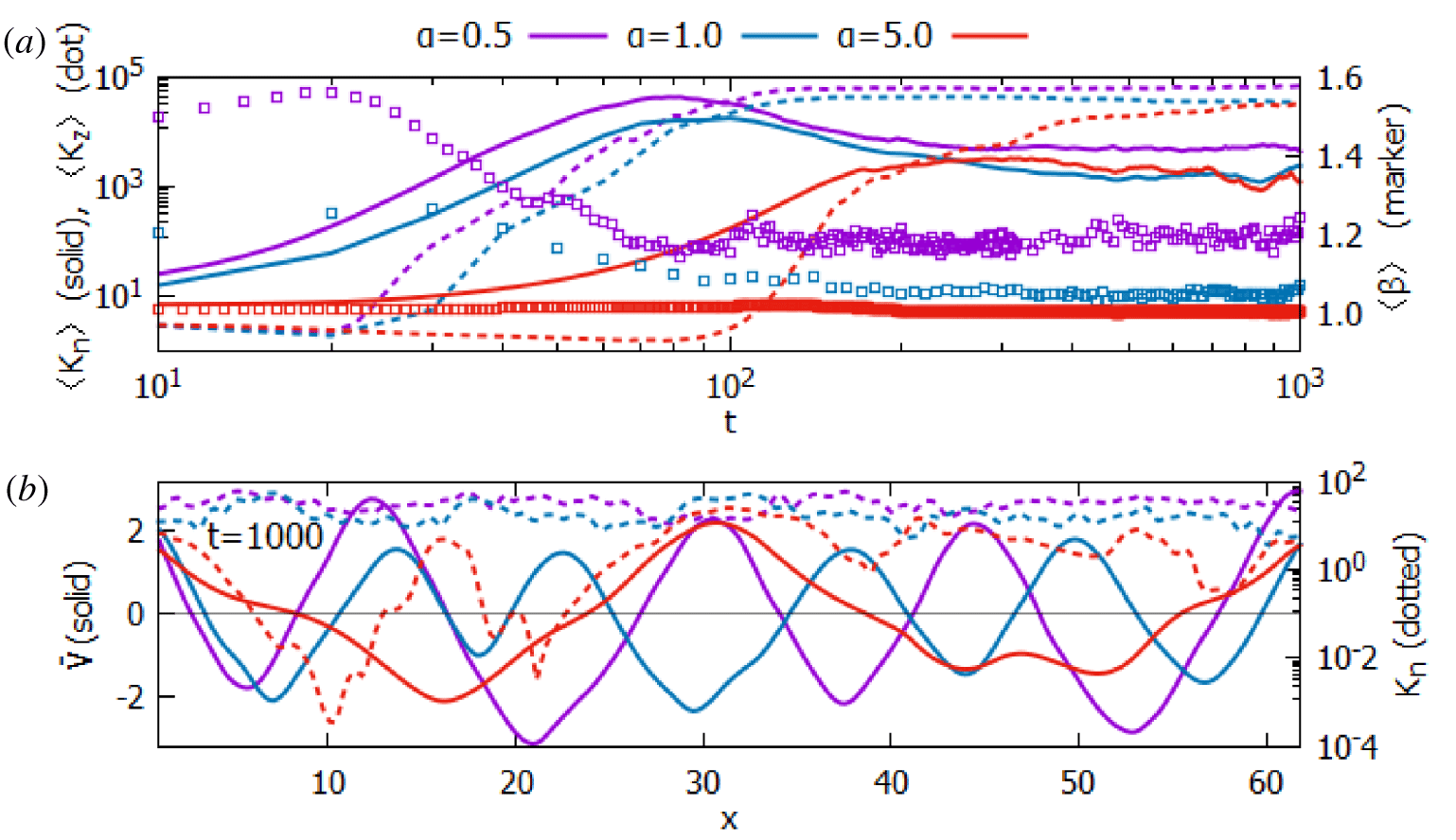
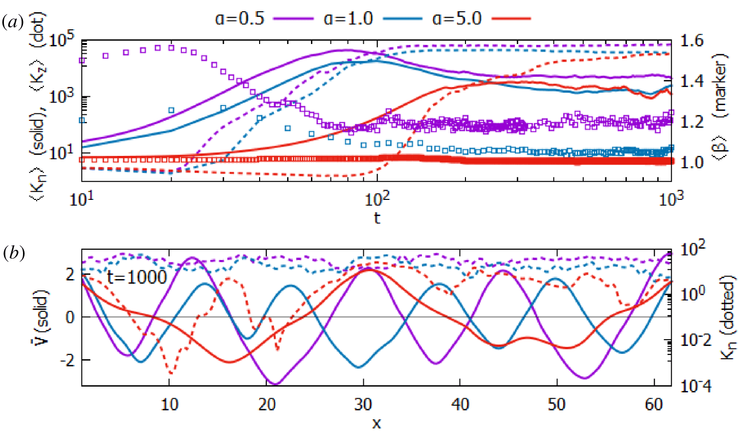
Evolution toward quasi-steady state and the profiles of the zonal field and the turbulence for $\unicode[STIX]{x1D6FC}=0.5$, 1.0 and 5.0. (a) Change in time of the zonal and non-zonal kinetic energies, $\langle K_{z}\rangle$ (dotted line) and $\langle K_{n}\rangle$ (solid line), and $\langle \unicode[STIX]{x1D6FD}\rangle$ (with markers) which is the square root of the ratio between the non-zonal particle density and the potential energies. (b) The zonal flow $\bar{V}$ and the non-zonal kinetic energy $K_{n}$ summed over the $y$ axis.

3 Results and discussion

Equations (2.1) and (2.2) are numerically integrated in time on the BOUT$++$ platform (Dudson et al. Reference Dudson, Umansky, Xu, Snyder and Wilson2009). A square domain of length $L=20\unicode[STIX]{x03C0}$ is turned into the set of $256^{2}$ equally spaced grid points with the spacing $\unicode[STIX]{x0394}x=\unicode[STIX]{x0394}y\approx 0.25$. For the differentials in space, a fourth-order finite-difference scheme is used and the advance in time is made possible by PVODE with adaptive time stepping. In order to treat the Poisson brackets, the Arakawa scheme (Arakawa Reference Arakawa1966) is adopted. The simulation starts from the initial state of zero density perturbation and non-zero pseudo-random vorticity $\unicode[STIX]{x1D714}(x,y)=10^{-2}\sum _{j,k=1}^{15}\cos (2j\unicode[STIX]{x03C0}x/L+\unicode[STIX]{x1D703}_{j})\cos (2k\unicode[STIX]{x03C0}y/L+\unicode[STIX]{x1D703}_{k})$ with random phase constants $\unicode[STIX]{x1D703}$. The fluctuations are enforced to satisfy the periodic boundary conditions. We consider the cases of a near-adiabatic electron response so that the parameter $\unicode[STIX]{x1D6FC}$ in (2.1) and (2.2) is set to 5 if not stated otherwise. The coefficient of the fourth-order hyper-diffusion is $\unicode[STIX]{x1D708}=1\times 10^{-4}$ for the non-zonal fields. The diffusion coefficient of the zonal fields is $\bar{\unicode[STIX]{x1D708}}=1\times 10^{-2}$. Zonal flow is self-consistently generated from the non-zonal fields by the dynamics of (2.1) and (2.2). The simulation result for the case of $\unicode[STIX]{x1D6FC}=5.0$ is most interesting so that this result is mainly highlighted and compared to the case where the zonal flow is specified to be a sinusoidal profile.

Gross features of the simulations with $\unicode[STIX]{x1D6FC}=0.5$, 1.0 and 5.0 are plotted in figure 1. In the upper part the evolutions toward quasi-steady state are shown of the kinetic energies of the zonal $\langle K_{z}\rangle =\int \text{d}x\,\text{d}y\bar{V}(x)^{2}/2$ and the non-zonal $\langle K_{n}\rangle =\int \text{d}x\,\text{d}y|\unicode[STIX]{x1D6FB}_{\bot }\tilde{\unicode[STIX]{x1D711}}|^{2}/2$ flows and $\langle \unicode[STIX]{x1D6FD}\rangle =\sqrt{\int \text{d}x\,\text{d}y{\tilde{n}}^{2}/\int \text{d}x\,\text{d}y\tilde{\unicode[STIX]{x1D711}}^{2}}$, which represents a global measure for the adiabaticity. It is found that the non-zonal fluctuations grow initially and the zonal flows become excited out of the non-zonal turbulence. For smaller $\unicode[STIX]{x1D6FC}$, the linear growth of the non-zonal fluctuations is faster, the zonal flows appear earlier and the fluctuations saturate sooner. By the time $t=10^{3}$, $\langle K_{z}\rangle$ becomes greater than $\langle K_{n}\rangle$ by more than an order of magnitude and both of them saturate at higher levels for smaller $\unicode[STIX]{x1D6FC}$. $\langle \unicode[STIX]{x1D6FD}\rangle$ becomes saturated at larger value for smaller $\unicode[STIX]{x1D6FC}$. This is because the main destabilizing factor in the HWM is the adiabaticity between $\tilde{\unicode[STIX]{x1D711}}$ and ${\tilde{n}}$, which is inversely related to $\unicode[STIX]{x1D6FC}$. In the lower part of figure 1 the profiles of the zonal flow and the distributions of the non-zonal kinetic energy $K_{n}(x)=\int \text{d}y|\unicode[STIX]{x1D6FB}_{\bot }\tilde{\unicode[STIX]{x1D711}}|^{2}/2$ are plotted for the same three $\unicode[STIX]{x1D6FC}$ at $t=10^{3}$.

Peak speed of the zonal flows is around 2 and $\bar{V}$ values vary quasi-periodically across $x$ with a different periodicity between $L_{x}/2$ and $L_{x}/5$ depending on $\unicode[STIX]{x1D6FC}$. This is because most non-zonal energy is carried by the large-scale (wavenumber $k\ll 1$ in $x$) fluctuations. For $\unicode[STIX]{x1D6FC}=5.0$ zonal flow mostly extracts energy from the period-two non-zonal fluctuations. Right portion of $\bar{V}$ of $\unicode[STIX]{x1D6FC}=5.0$, by the way, needs more time to saturate (see figure 3). A striking difference between the less adiabatic cases of $\unicode[STIX]{x1D6FC}=0.5$ and 1.0 and the highly adiabatic case of $\unicode[STIX]{x1D6FC}=5.0$ is the turbulence distribution. In the former cases the turbulence is widespread, not particularly localized where $|\bar{V}|$ is large and its peaks are not prominent. For $\unicode[STIX]{x1D6FC}=5.0$, in contrast, the non-zonal fluctuations are well separated, being localized where $\bar{V}$ is fast at $x\approx 16$ and 30. Incidentally, the right part of $\bar{V}$ around $x\approx 47$ has not yet reached the stationary state by $t=10^{3}$. Since such localization is unique and interesting, further analysis of the results in the case of $\unicode[STIX]{x1D6FC}=5.0$ continues.

Such localization by the zonal flow has been reported in the presence of the zonal flow being forced externally, instead of being self-consistently derived from the mHWE (Kim et al. Reference Kim, Min and An2019b). A sinusoidally varying zonal flow $\bar{V}(x)=2\cos (4\unicode[STIX]{x03C0}x/L)$ is enforced and the non-zonal fluctuations are computed accordingly. The zonal density, in contrast, is allowed to evolve based on (2.1) and (2.2). Forced ZF model takes advantage of analytical understandings of the linear state in the presence of the zonal flow. It was reported that the linear eigenmodes are localized around a positive peak of $\bar{V}$ (Kim, Min & An Reference Kim, Min and An2018). After an initial exponential growth of the perturbation, the level of the non-zonal fluctuations increases, the nonlinear $\boldsymbol{E}\times \boldsymbol{B}$ advection terms in (2.3) and (2.4) become dominant and the growth of the zonal density follows (Kim et al. Reference Kim, Min and An2019b). As a result, the growth of the fluctuations slows down and by the time $t=10^{3}$ they saturate.

Figure 2.

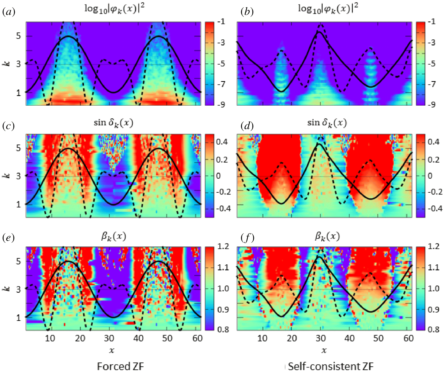
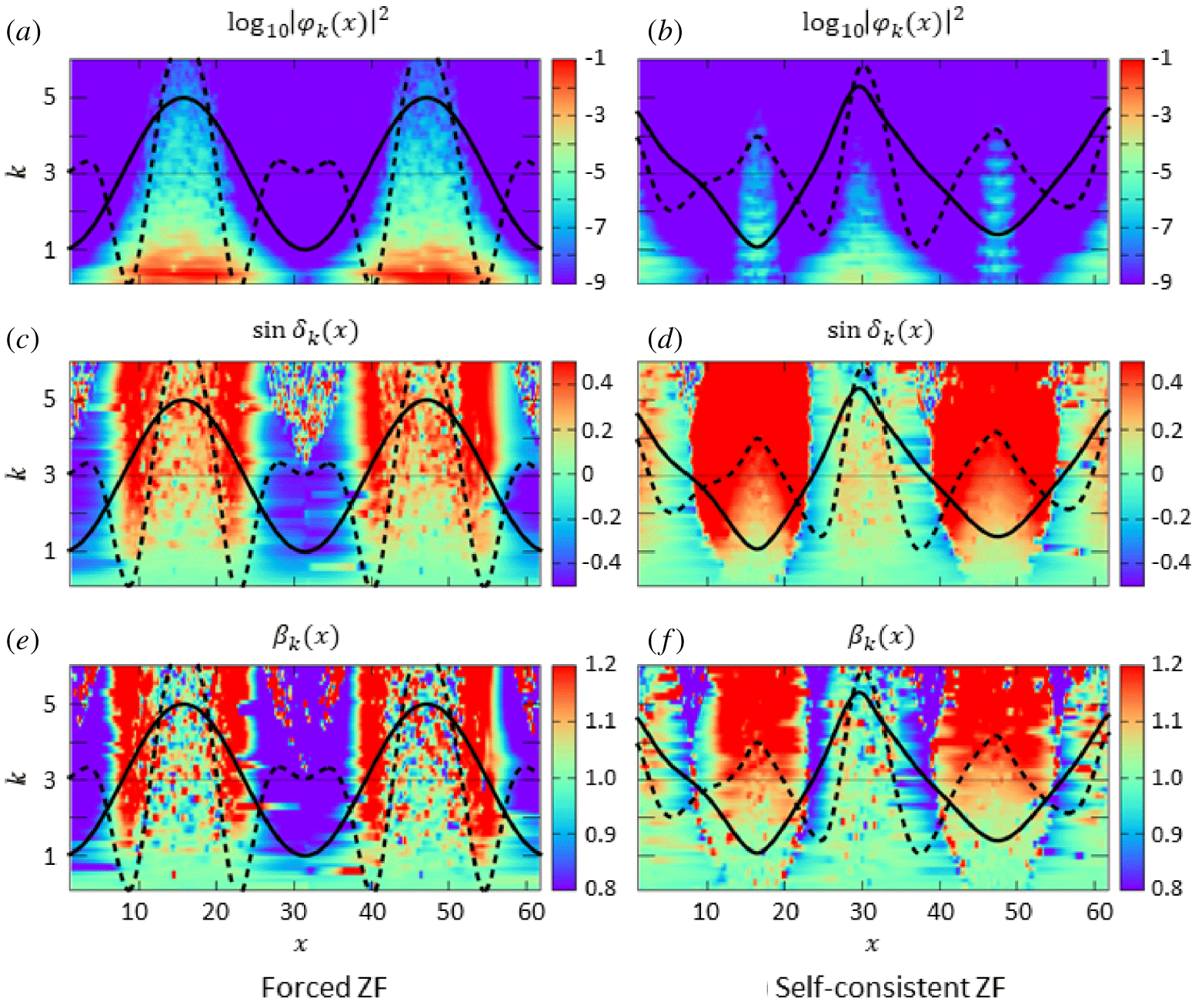
Self-consistent non-zonal turbulence of $\unicode[STIX]{x1D6FC}=5$ (b,d,f) is compared to the case of externally forced zonal flow $\bar{V}=-2\cos (x/5)$ (a,c,e) at a quasi-steady state around $t=2\times 10^{3}$. From panel (a,b): colour maps in the $x{-}k$ plane of the turbulence distribution $|\tilde{\unicode[STIX]{x1D711}}_{k}|^{2}$, the sine of the cross-phase $\sin \unicode[STIX]{x1D6FF}_{k}$ and the ratio between the particle density and the potential $\unicode[STIX]{x1D6FD}_{k}=|{\tilde{n}}_{k}|/|\tilde{\unicode[STIX]{x1D711}}_{k}|$. Superimposed are the zonal flow (black solid line), in the scale between $-3$ and 3, and the zonal-density gradient (black dotted line) in the scale between $-0.6$ and 0.6.

Figure 3.

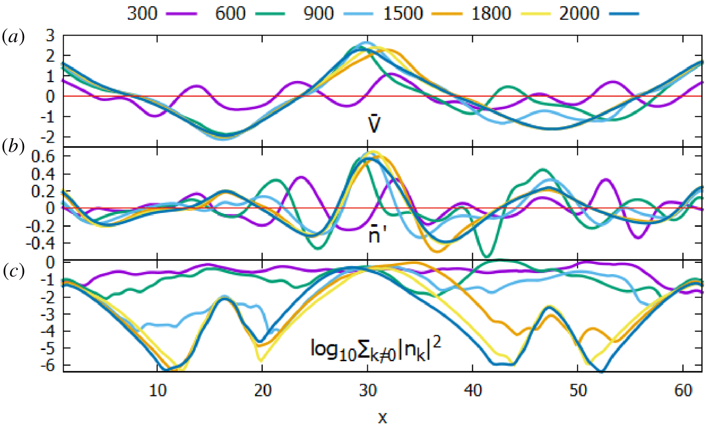
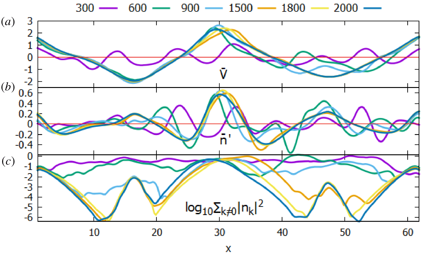
The profiles of the zonal flow $\bar{V}$ (a), the zonal-density gradient $\bar{n}^{\prime }$ (b) and the non-zonal density fluctuations $\sum _{k}|{\tilde{n}}_{k}|^{2}$ (c) at representative times $t=3\times 10^{2}$, $6\times 10^{2}$, $9\times 10^{2}$, $1.5\times 10^{3}$, $1.8\times 10^{3}$ and $2\times 10^{3}$.

Results of two simulations with ZF either being forced or self-consistent in the case of $\unicode[STIX]{x1D6FC}=5.0$ are compared in figure 2. Spectral distributions of $\tilde{\unicode[STIX]{x1D711}}_{k}(x)$, $\sin \unicode[STIX]{x1D6FF}_{k}(x)$ and $\unicode[STIX]{x1D6FD}_{k}(x)$ around $t=10^{3}$ for the forced case and around $t=2\times 10^{3}$ for the self-consistent case are shown in the figure. In panel (a,b) it is shown that, in both cases, the fluctuations are well separated and are localized where $\bar{V}$ (black solid line in the figure) is a positive (along the electron diamagnetic drift) peak. Similarity between the two cases stops, however, where $\bar{V}$ is a negative peak: turbulence is localized in the relatively narrow region in the dynamically consistent case while it is absolutely weak in the forced case. This is because, in the self-consistent case, fast ZF needs strong turbulence as an energy supplier in contrast to the forced fast ZF. In the steady state of the self-consistent turbulence the Reynolds stress supports the zonal flow by (2.7), $\bar{\unicode[STIX]{x1D6F1}}^{\prime }=-\bar{\unicode[STIX]{x1D708}}\unicode[STIX]{x2202}_{x}^{4}\bar{V}$. Since the supplied power by the non-zonal fluctuations is $-\bar{V}\bar{\unicode[STIX]{x1D6F1}}^{\prime }$, $\bar{\unicode[STIX]{x1D6F1}}^{\prime }$ needs to be positive and peaked where $\bar{V}$ is a negative local peak. As a result, the zonal-density gradient $\bar{n}^{\prime }$ (black dotted line in the figure) is almost zero in the forced case (2.8) whereas it develops a positive peak in the self-consistent case, which will be explained in the next paragraph. In the forced case, contrary to the conventional wisdom, the turbulence level at a negative peak of $\bar{V}$ where $\bar{V}^{\prime }=0$ is weaker than where $\bar{V}^{\prime }$ is large ($x=7.5\unicode[STIX]{x03C0}$ and $12.5\unicode[STIX]{x03C0}$). This is because the zonal flow is already set up when the plasma equilibrium is disturbed. Linear study finds the perturbation decays fastest where $\bar{V}$ is a negative maximum (Kim et al. Reference Kim, Min and An2018). In the nonlinear phase, therefore, the nonlinear effect is not large and turbulence is kept small even in the saturated state if $\bar{V}$ is large enough (Kim et al. Reference Kim, Min and An2019b). The energy spectrum depends on the sign of $\bar{V}$ at the peak locations: where positive around $x=30$ the fluctuations of small $k<1$ are energetic whereas at negative peaks the energy is spread over the fluctuations with wider range of $k$ up to around 2. Spectral distributions are more closely examined below. In figure 2(c,d) $\unicode[STIX]{x1D6FF}_{k}$ of the energetic fluctuations are small and positive where $\bar{V}$ is a positive peak for both cases of forced and self-consistent ZFs. Around where $\bar{V}$ is a negative peak, $\unicode[STIX]{x1D6FF}_{k}$ values in the self-consistent case are also positive so that the plasma needs to be unstable to balance the damping. In the narrow layer where $|\tilde{\unicode[STIX]{x1D711}}_{k}|^{2}$ is negligibly small, $\unicode[STIX]{x1D6FF}_{k}$ are negative. It is consistent with the fact that the fluctuation is weak because positive $\unicode[STIX]{x1D6FF}_{k}$ drives the density fluctuations unstable in (2.6). In the forced case, the region of weak fluctuations where $\bar{V}$ is a negative peak accordingly corresponds to negative $\unicode[STIX]{x1D6FF}_{k}$. Since $\tilde{\unicode[STIX]{x1D711}}$ is driven unstable if $\unicode[STIX]{x1D6FD}_{k}>1$ (2.5), one finds in figure 2(e,f) that $\unicode[STIX]{x1D6FD}_{k}<1$ in the regions of weak turbulence for both cases.

Figure 4.

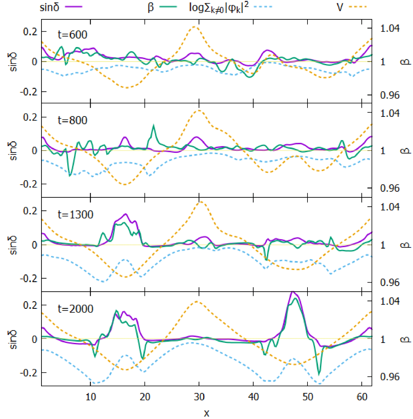
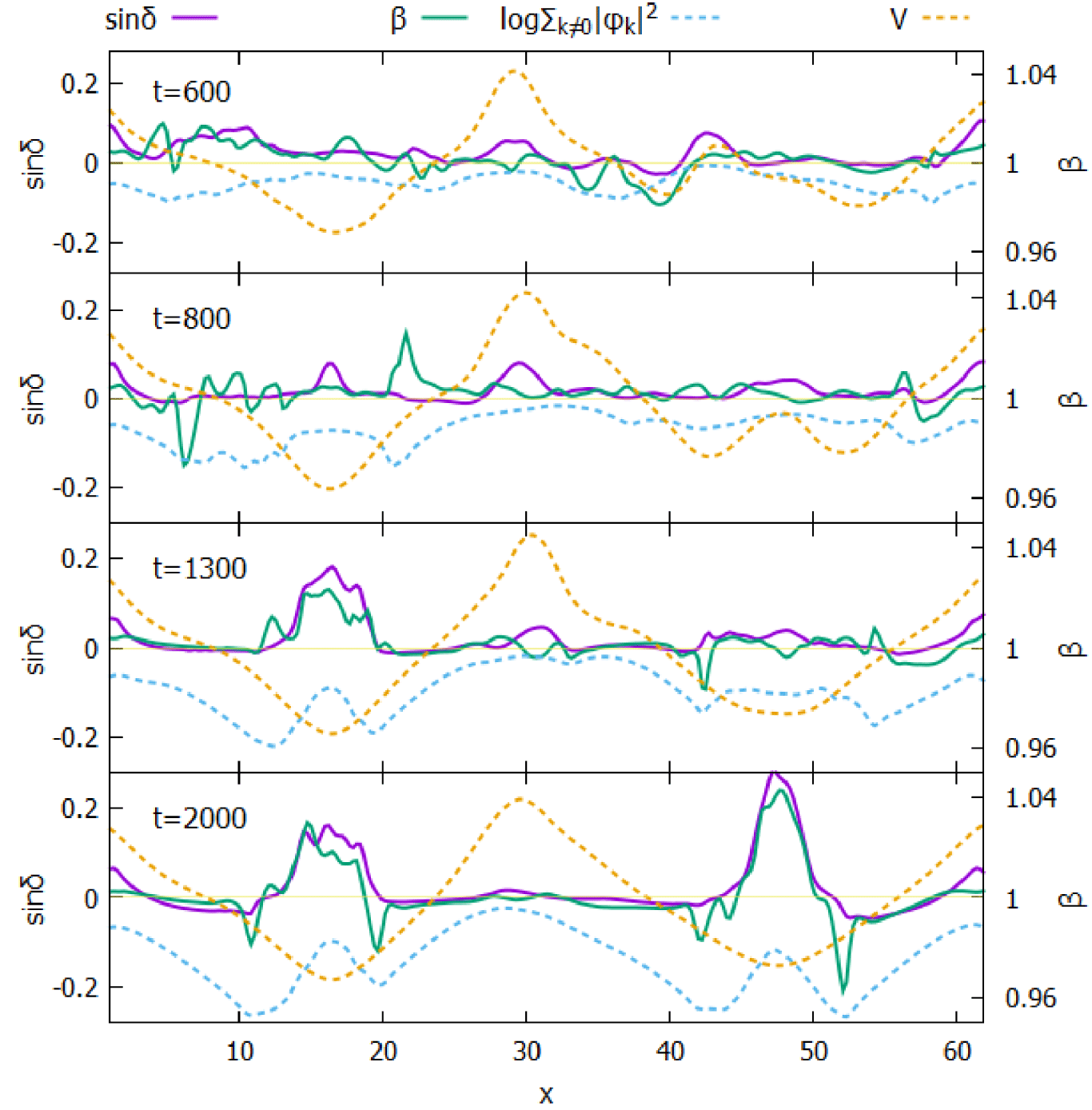
The profiles of 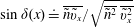$\sin \unicode[STIX]{x1D6FF}(x)\doteq \overline{{\tilde{n}}\tilde{v}_{x}}/\sqrt{\overline{{\tilde{n}}^{2}}\,\overline{\tilde{v}_{x}^{2}}}$ and 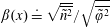$\unicode[STIX]{x1D6FD}(x)\doteq \sqrt{\overline{{\tilde{n}}^{2}}}/\sqrt{\overline{\tilde{\unicode[STIX]{x1D711}}^{2}}}$ at representative times $t=6\times 10^{2}$, $8\times 10^{2}$, $1.3\times 10^{3}$ and $2\times 10^{3}$. Superimposed are the zonal flow $\bar{V}$ (yellow dotted line) and the fluctuation distribution (blue dotted line) respectively scaled to fit in the frames.

Turbulence in the case of a dynamically generated ZF is further analysed for $\unicode[STIX]{x1D6FC}=5.0$ in the following. Figure 3 shows the profiles of $\bar{V}$ (a), $\bar{n}^{\prime }$ (b) and the non-zonal-density fluctuations $\sum _{k}|{\tilde{n}}_{k}|^{2}$ (c) at representative times $t=3\times 10^{2}$, $6\times 10^{2}$, $9\times 10^{2}$, $1.5\times 10^{3}$, $1.8\times 10^{3}$ and $2\times 10^{3}$. Part of $\bar{V}$ profile around $x=16$ becomes quasi-stationary by the time $t=600$ whereas the right part of the profile around $x=47$ does not reach quasi-steady state until $t=1500$ while the middle portion around $x=30$ keeps oscillating in time. Similarly to $\bar{V}$, $\bar{n}^{\prime }$ and $\sum _{k\not =0}|{\tilde{n}}_{k}|^{2}$ evolve in time as the right part settles down later, lagging the left, while the central region oscillates. It is interesting to note that there are twice as many peaks of $\bar{n}^{\prime }$ as of $\bar{V}$ and, unlike $\bar{V}$, only the positive peaks of $\bar{n}^{\prime }$ are coincident with the locations of the localized turbulence. In the steady state, particle transport supports the zonal-density profile from (2.8), $\bar{\unicode[STIX]{x1D6E4}}=-\bar{\unicode[STIX]{x1D708}}\unicode[STIX]{x2202}_{x}^{3}\bar{n}$. Where $\bar{\unicode[STIX]{x1D6E4}}$ is positive and narrowly peaked symmetrically around $x_{0}$, $\bar{n}^{\prime \prime \prime }$ is negatively peaked and $\bar{n}^{\prime \prime }$ crosses zero from positive to negative at $x_{0}$. Therefore $\bar{n}^{\prime }$ is positively peaked at $x_{0}$. If $\bar{n}$ is diffusively dissipated, $\unicode[STIX]{x1D708}_{2}\bar{n}^{\prime \prime }$, instead of $-\bar{\unicode[STIX]{x1D708}}\unicode[STIX]{x2202}_{x}^{4}\bar{n}$, the balance would be $\bar{\unicode[STIX]{x1D6E4}}=\unicode[STIX]{x1D708}_{2}\bar{n}^{\prime }$ and the turbulence would be still strong at the positive peaks of $\bar{n}^{\prime }$. Non-zonal fluctuations show an interesting feature during relaxation. Both in the left and right parts, depending on the locations, the fluctuations decay in time with different rates: in the regions of peak zonal flow they decrease slower and reach a stationary state sooner. Since the fluctuations in the narrow regions surrounding the peaks of $\bar{V}$ keep declining before saturation, fluctuations are trapped in the regions around the peaks of $\bar{V}$ and they are separated from each other.

Plots in figure 4 represent the degree of difference between $\tilde{\unicode[STIX]{x1D711}}$ and ${\tilde{n}}$, which is the cause of the instability. The profiles of 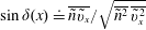$\sin \unicode[STIX]{x1D6FF}(x)\doteq \overline{{\tilde{n}}\tilde{v}_{x}}/\sqrt{\overline{{\tilde{n}}^{2}}\,\overline{\tilde{v}_{x}^{2}}}$ and 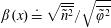$\unicode[STIX]{x1D6FD}(x)\doteq \sqrt{\overline{{\tilde{n}}^{2}}}/\sqrt{\overline{\tilde{\unicode[STIX]{x1D711}}^{2}}}$, where over-lines means summations over the $y$ axis, are shown in figure 4 at times $t=6\times 10^{2}$, $8\times 10^{2}$, $t=1.3\times 10^{3}$ and $2\times 10^{3}$. Also included in the figures are the zonal flow $\bar{V}$ (yellow dotted line) and the fluctuation distribution (blue dotted line) that are properly rescaled to fit. By $t=10^{3}$ both $\sin \unicode[STIX]{x1D6FF}$ and $\unicode[STIX]{x1D6FD}$ become pronounced as high as 0.2 and 1.04 respectively around $x=16$, where $\bar{V}$ is negative and fast and the turbulence is locally peaked, and stay almost unchanged afterwards. Later, by $t=1.6\times 10^{3}$, they also become locally large around $x=47$ where $\bar{V}$ is another negative maximum. This suggests that the degree of deviation from the adiabatic state, however small but finite, is important in forming the profiles of the zonal flow that is fast and negative and the turbulence. Another point to notice is that, where the zonal flow changes directions, $\sin \unicode[STIX]{x1D6FF}<0$ and $\unicode[STIX]{x1D6FD}<1$ by the time $t=2\times 10^{3}$. It is checked that the feature holds up to $t=2\times 10^{4}$.

Figure 5.

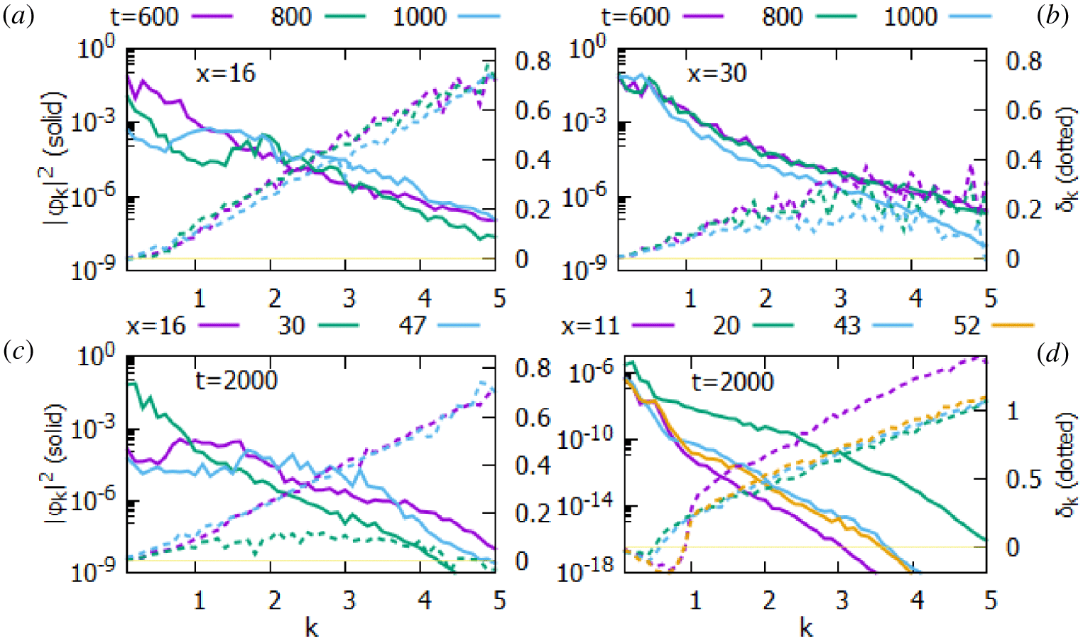
Spectrum and the cross-phase where the turbulence is either locally strong or weak: at $x=16$ (a), where $\bar{V}$ is negative and large, and $x=30$ (b) where $\bar{V}$ is positive and large, each averaged over a time interval $\unicode[STIX]{x0394}t=200$ centred at $t=6\times 10^{2}$, $8\times 10^{2}$ and $10^{3}$, respectively. Spectra and the cross-phases at a quasi-steady state (averaged between $t=1.8\times 10^{3}$ and $2\times 10^{3}$) where the turbulence level is locally strong (c) and negligibly weak (d).

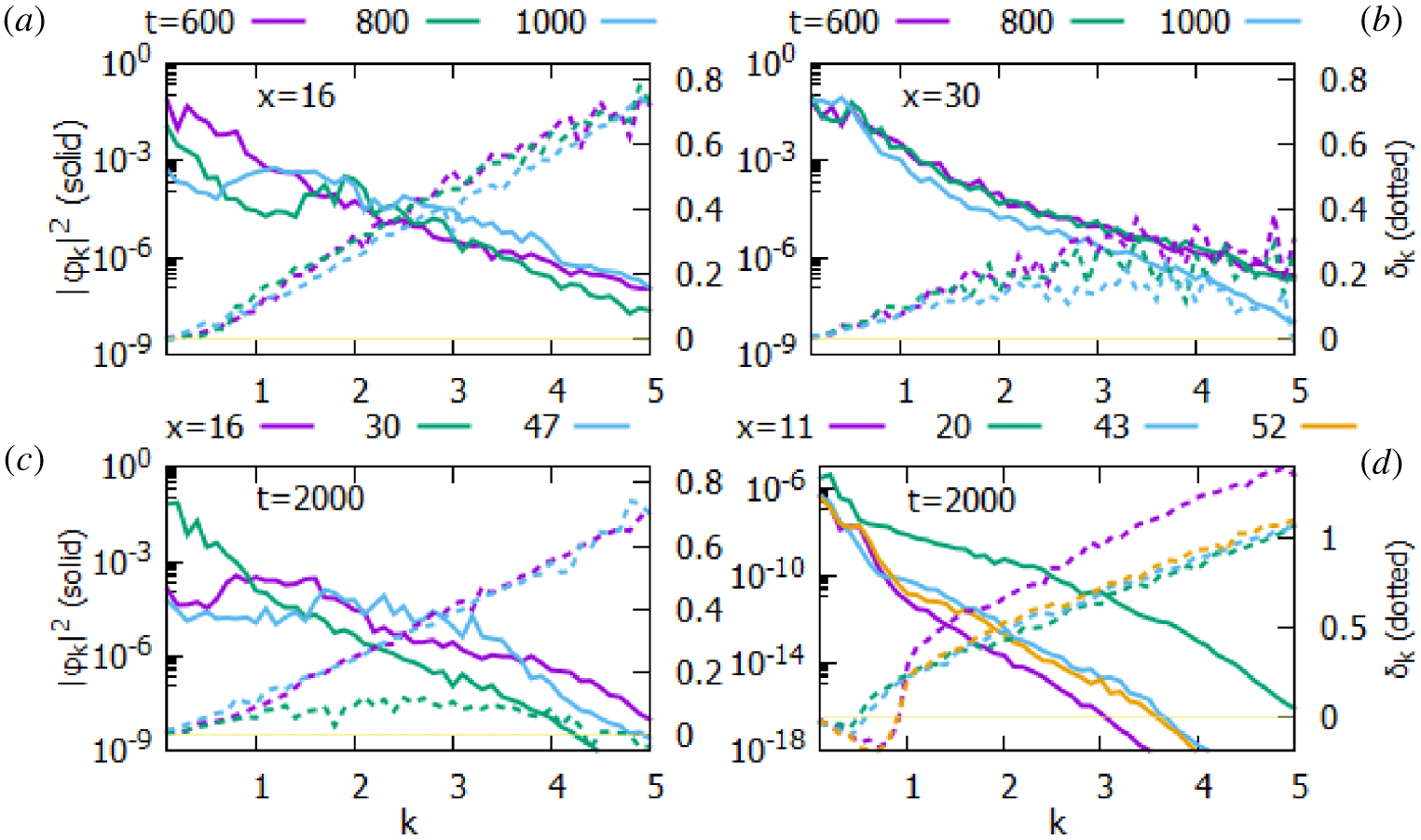
In order to further examine the characteristics of the turbulence, the spectral distribution of $|\tilde{\unicode[STIX]{x1D711}}_{k}|^{2}$ and $\unicode[STIX]{x1D6FF}_{k}$ at significant locations are shown in figure 5. Near $x=16$ the energy spectrum changes from being peaked near $k\ll 1$ at $t=600$ to being broadly peaked around $1\leqslant k\leqslant 2$ after the appearance of a sub-peak around $k\approx 2$ at $t=800$ (a). By $t=2\times 10^{3}$ the energy spectrum at $x=47$ similarly becomes broad in $k$, not sharply peaked at low $k$ (c). Yet the spectrum at $x=30$ remains peaked near the lowest $k$ (b,c). At all three locations $\unicode[STIX]{x1D6FF}_{k}$ is found to increase in terms of $k$. Since $\unicode[STIX]{x1D6FF}_{k}$ at $x=30$ is smaller than at $x=16$, the effective cross-phase at $x=16$ and 47 is larger than at $x=30$ (see figure 4). Also shown are the spectra at the locations of minimal fluctuation, $x=11$, 20, 43 and 52, at $t=2\times 10^{3}$ (d). Albeit small, they are peaked at the lowest possible $k$ and $\unicode[STIX]{x1D6FF}_{k}$ of $k\ll 1$ is found to be negative.

Figure 6.

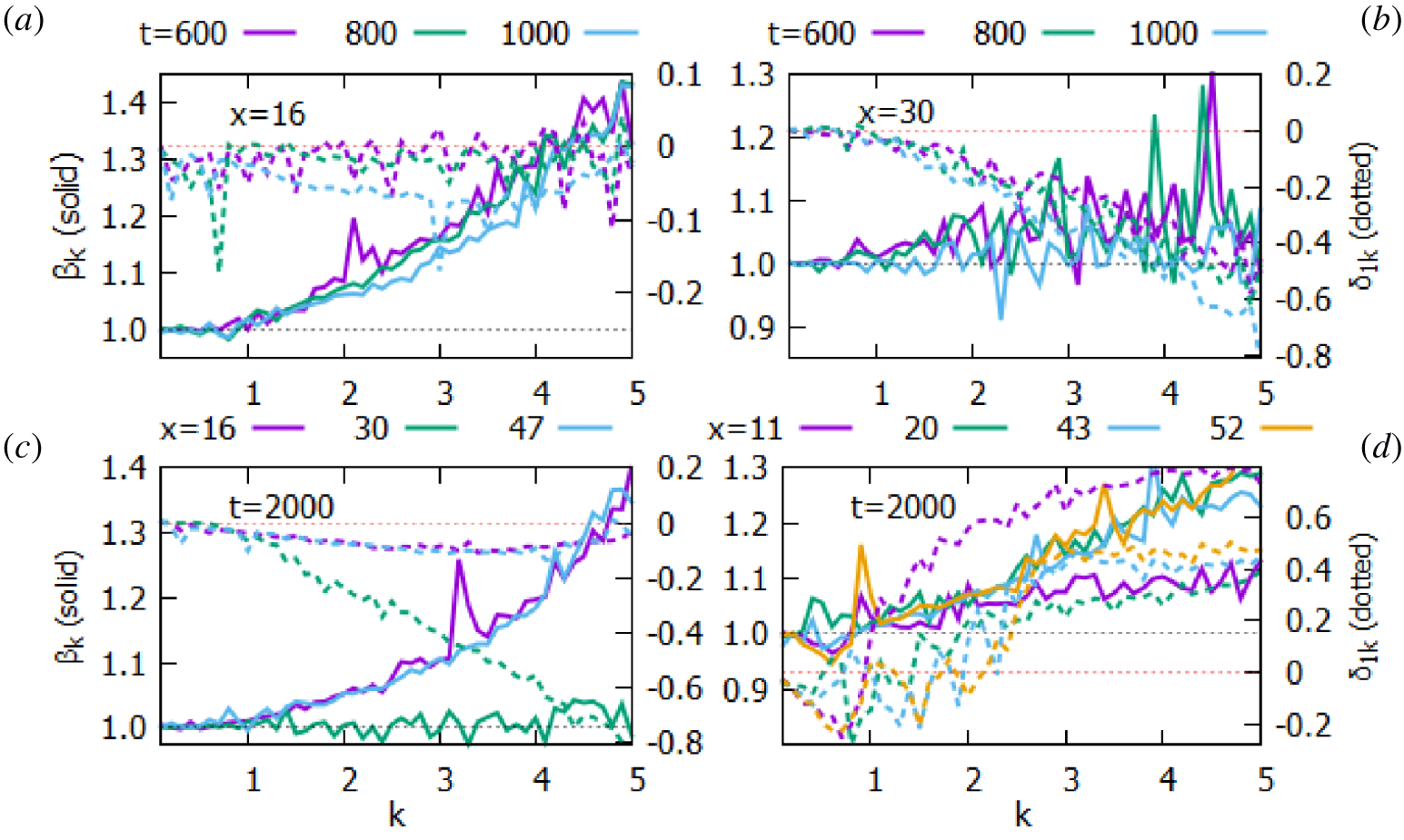
The ratio $\unicode[STIX]{x1D6FD}_{k}=|{\tilde{n}}_{k}|/|\tilde{\unicode[STIX]{x1D711}}_{k}|$ and the cross-phase $\unicode[STIX]{x1D6FF}_{1k}$, that is explicitly dependent on the zonal fields, where the turbulence is either locally strong or weak: at $x=16$ (a), where $\bar{V}$ is negative and large, and $x=30$ (b) where $\bar{V}$ is positive and large, each averaged over a time interval $\unicode[STIX]{x0394}t=200$ centred at $t=6\times 10^{2}$, $8\times 10^{2}$ and $10^{3}$. $\unicode[STIX]{x1D6FD}_{k}=|{\tilde{n}}_{k}|/|\tilde{\unicode[STIX]{x1D711}}_{k}|$ and $\unicode[STIX]{x1D6FF}_{1k}$ at a quasi-steady state (averaged between $t=1.8\times 10^{3}$ and $2\times 10^{3}$) where the turbulence level is locally strong (c) and negligibly weak (d).

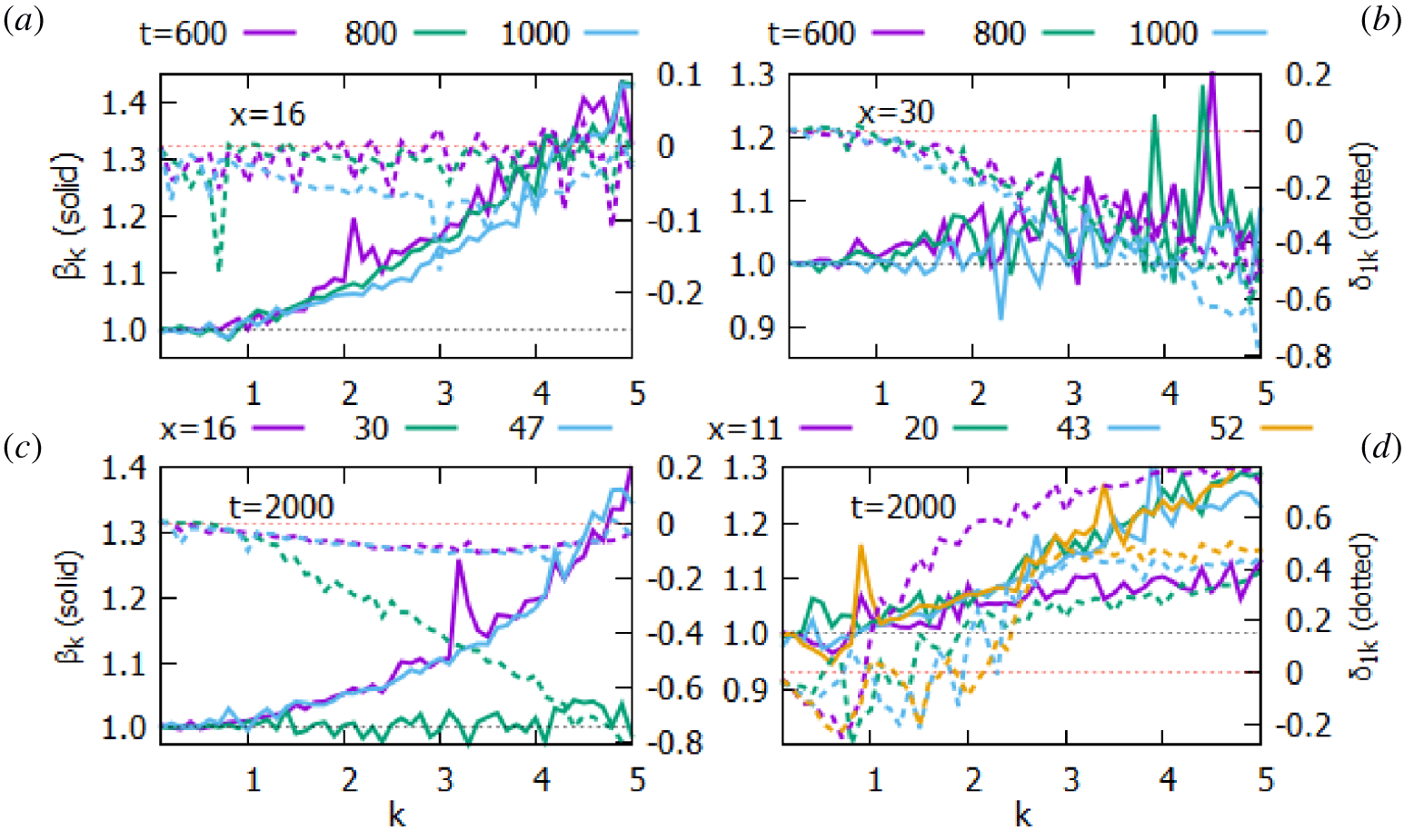
In figure 6 $\unicode[STIX]{x1D6FD}_{k}$ values at $x=16$ and $47$ are larger than at $x=30$, which are nearly 1 all over $k$. Also plotted in the figure is the spectral distribution of $\unicode[STIX]{x1D6FF}_{1k}$ obtained by the subtraction $\unicode[STIX]{x1D6FF}_{k}-\unicode[STIX]{x1D6FF}_{0k}$, which contains explicit contributions of $\bar{V}$ and $\bar{n}^{\prime }$. At a quasi-steady state at $t=2\times 10^{3}$ it is found that $\unicode[STIX]{x1D6FF}_{1k}$ of the fluctuations at $x=16$, 47 and 30 are all negative (c). This means that the zonal fields $\bar{V}$ and $\bar{n}^{\prime }$ reduce the cross-phase around the peaks of $\bar{V}$. As a result the instability is tamed and the fluctuation level becomes lower. Since the fluctuation energy is concentrated in low-$k$ modes at $x=30$, such reduction of the cross-phase is not as relevant as at $x=16$ and 47. It is clear that $\unicode[STIX]{x1D6FF}_{k}$ at the locations of minimal fluctuation is negative for $k<1$ because of $\unicode[STIX]{x1D6FF}_{k}$ being negative (d).

In summary, for $\unicode[STIX]{x1D6FC}=5.0$, the fluctuations are limited around the peaks of the zonal flow that is generated dynamically by the non-zonal turbulence. Depending on the direction of the zonal flow, the fluctuations exhibit different characteristics: at a positive peak of $\bar{V}$ low-$k$ fluctuations are strong whereas most energy is carried by the fluctuations of $1\leqslant k\leqslant 2$ at a negative peak. As a result, the turbulence around the region of positive peak of $\bar{V}$ is present in a wider region than that of the negative peak of $\bar{V}$ if the fluctuations are not far from isotropic. Since the cross-phase increases with $k$, the fluctuations where $\bar{V}$ is a negative peak are effectively further away from being adiabatic than where $\bar{V}$ is a positive peak. In between the regions of fast $\bar{V}$ exist narrow layers of negligible fluctuations. They are formed by stabilization of the energetic fluctuations through the reductions of $\unicode[STIX]{x1D6FF}_{k}$ to be negative and of $\unicode[STIX]{x1D6FD}_{k}$ below 1 by the zonal fields.