1 Introduction
Vortex rings are one of the fundamental vortices which appear in various flows. They are formed when fluid is ejected into a quiescent fluid from a circular hole whose size ranges from human lips to volcanoes. They also appear as coherent structures in a circular jet. An important feature of vortex rings is that vortex tubes have curvature, which distinguishes them from line vortices. Curvature has significant effects on the dynamics of a vortex ring. A vortex ring propagates owing to self-induced velocity due to curvature (Saffman Reference Saffman1992; Fukumoto & Moffatt Reference Fukumoto and Moffatt2000). More importantly, curvature deforms the core of a vortex ring to give rise to short-wave instabilities (Hattori & Fukumoto Reference Hattori and Fukumoto2003; Fukumoto & Hattori Reference Fukumoto and Hattori2005).
Currently, two types of short-wave instabilities are known for vortex rings: elliptic instability and curvature instability. The elliptic instability of a vortex ring was established about four decades ago; Widnall & Tsai (Reference Widnall and Tsai1977) showed that the strain induced on the core of a vortex ring by itself resonates with two neutral waves to give rise to an instability. The essential mechanism had been understood for a strained line vortex by Moore & Saffman (Reference Moore and Saffman1975) and Widnall & Tsai (Reference Widnall and Tsai1976). Their theoretical results were in reasonable agreement with the experimental results of Widnall & Sullivan (Reference Widnall and Sullivan1973), which supports that the observed growth of bending waves is due to the elliptic instability. On the other hand, the curvature instability was first found theoretically by Hattori & Fukumoto (Reference Hattori and Fukumoto2003) and Fukumoto & Hattori (Reference Fukumoto and Hattori2005); it is caused by the dipolar field which is self-induced on the core of a vortex ring and resonates with two neutral waves as in the case of elliptic instability. One of the important differences between the elliptic and curvature instabilities is the set of azimuthal wavenumbers of the coupled waves:
 $(m,m+2)$
, where
 $m$
is an integer, in the elliptic instability and
 $(m,m+1)$
in the curvature instability. The curvature instability has been shown to exist theoretically also for Hill’s spherical vortices (Hattori & Hijiya Reference Hattori and Hijiya2010) and helical vortices (Hattori & Fukumoto Reference Hattori and Fukumoto2009, Reference Hattori and Fukumoto2010, Reference Hattori and Fukumoto2011, Reference Hattori and Fukumoto2012, Reference Hattori and Fukumoto2014).
It should be pointed out that the above results for the curvature instability and the results of Widnall & Tsai (Reference Widnall and Tsai1977) are obtained for Kelvin’s vortex ring for which vorticity is constant inside the core at the leading order of perturbation expansion and vanishes outside the core. However, the vortex rings observed in experiments usually have smooth vorticity distributions which are often approximated by Gaussian distributions. Recently, Blanco-Rodríguez & Le Dizès (Reference Blanco-Rodríguez and Le Dizès2016) and Blanco-Rodríguez & Le Dizès (Reference Blanco-Rodríguez and Le Dizès2017) have shown theoretically that vortex rings which have Gaussian distributions of azimuthal vorticity and velocity at the leading order are also subjected to elliptic and curvature instabilities. They found that some important features of the instabilities are quite different from those of Kelvin’s vortex ring. In fact, characteristics of the waves on the Gaussian vortices change dramatically when there exists a critical layer whose radius satisfies
 $$\begin{eqnarray}\displaystyle \unicode[STIX]{x1D714}-ku_{\unicode[STIX]{x1D719}}^{(0)}(r)-m\unicode[STIX]{x1D6FA}^{(0)}(r)=0, & & \displaystyle\end{eqnarray}$$
where
 $\unicode[STIX]{x1D714}$
is the oscillation frequency,
 $k$
and
 $m$
are the azimuthal and circumferential wavenumbers, respectively, and
 $u_{\unicode[STIX]{x1D719}}^{(0)}(r)$
and
 $\unicode[STIX]{x1D6FA}^{(0)}(r)$
are the azimuthal velocity and angular velocity distributions of the vortices, respectively; some waves are damped with non-vanishing decay rate in the inviscid limit and the dispersion curves are distorted (Le Dizès Reference Le Dizès2004; Fabre, Sipp & Jacquin Reference Fabre, Sipp and Jacquin2006). It turns out that the curvature instability is much more affected by the presence of critical layers than the elliptic instability. However, there do exist unstable modes of the curvature instability of which growth rates can be comparable to those of the elliptic instability in the presence of azimuthal velocity.
Experimental results on the instability of a vortex ring (Maxworthy Reference Maxworthy1972; Widnall & Sullivan Reference Widnall and Sullivan1973; Maxworthy Reference Maxworthy1977; Dazin, Dupont & Stanislas Reference Dazin, Dupont and Stanislas2006a ,Reference Dazin, Dupont and Stanislas b ; Thompson, Leweke & Hourigan Reference Thompson, Leweke and Hourigan2007; Gan, Nickels & Dawson Reference Gan, Nickels and Dawson2011) have not been fully understood in spite of many efforts; one of the reasons for this is that it is not always easy to measure detailed structures of destabilized vortex rings. Numerical results have revealed some features of the elliptic instability; a map of unstable modes has been obtained recently by Gargan-Shingles, Rudman & Ryan (Reference Gargan-Shingles, Rudman and Ryan2016) for vortex rings with swirl, where swirl implies the azimuthal or toroidal component of velocity in the present paper. See also Mao & Hussain (Reference Mao and Hussain2017) for transient growth and Shariff, Verzicco & Orlandi (Reference Shariff, Verzicco and Orlandi1994) for early pioneering work. However, clear evidence of the curvature instability has not been observed in experiments or numerical simulations as far as the authors know.
In the present paper, we study the linear instability of vortex rings by direct numerical simulation (DNS); Gaussian vortex rings which have swirl in general are considered as a base flow. Our first aim is to show that curvature instability exists in reality by DNS. After confirming its existence, the growth rates of the unstable eigenmodes are evaluated and compared to theoretical results. The structures of the unstable eigenmodes are also revealed. Nonlinear effects are also investigated to observe whether weakly nonlinear saturation occurs or not.
The paper is organized as follows. In § 2 we describe the numerical procedure. In § 3 some important features of numerically obtained base flow are presented. The linear stability results are shown in § 4, while nonlinear effects are studied in § 5. We conclude in § 6.
2 Numerical procedure
2.1 Outline
Flow model and coordinate system.

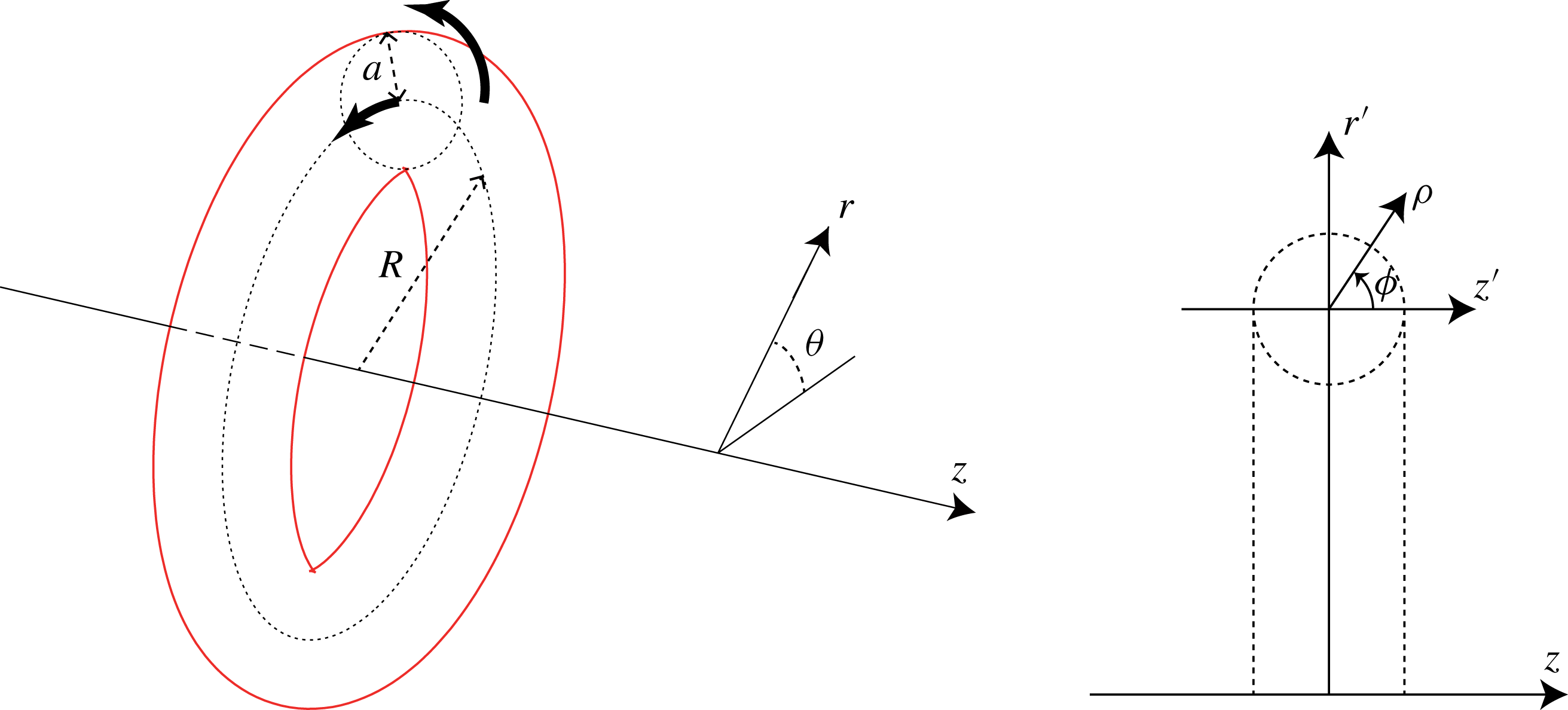
We consider the instability of a vortex ring in an incompressible viscous fluid (figure 1); the vortex ring has swirl in general. We take a cylindrical coordinate system
 $(r,\unicode[STIX]{x1D703},z)$
, where the axis of symmetry of the undisturbed vortex ring coincides with the
 $z$
axis. The numerical domain is
 $0\leqslant r\leqslant L_{r}$
,
 $0\leqslant \unicode[STIX]{x1D703}\leqslant 2\unicode[STIX]{x03C0}$
and
 $0\leqslant z\leqslant L_{z}$
. Periodic boundary conditions are assumed in the
 $z$
direction; the spatial period in the
 $z$
direction is taken sufficiently long so that the growth rate of an unstable mode is nearly the same as that for the infinitely long case.
The task consists of two steps: first, a quasi-steady base flow is obtained by solving the axisymmetric Navier–Stokes equations; next, the linearized Navier–Stokes equations are integrated for a sufficiently long time to obtain the most unstable mode when it exists. The details are described below.
2.2 Numerical methods
The incompressible Navier–Stokes equations are written as
 $$\begin{eqnarray}\displaystyle \frac{\unicode[STIX]{x2202}\boldsymbol{u}}{\unicode[STIX]{x2202}t}+\boldsymbol{u}\boldsymbol{\cdot }\unicode[STIX]{x1D735}\boldsymbol{u} & = & \displaystyle -\unicode[STIX]{x1D735}p+\unicode[STIX]{x1D708}\unicode[STIX]{x1D6FB}^{2}\boldsymbol{u},\end{eqnarray}$$
 $$\begin{eqnarray}\displaystyle \unicode[STIX]{x1D735}\boldsymbol{\cdot }\boldsymbol{u} & = & \displaystyle 0,\end{eqnarray}$$
where
 $\boldsymbol{u}$
is the velocity,
 $p$
is the pressure and
 $\unicode[STIX]{x1D708}$
is the kinematic viscosity; the constant density is set to
 $\unicode[STIX]{x1D70C}_{0}=1$
. To obtain a base flow, we set
 $\boldsymbol{u}=u(t,r,z)\boldsymbol{e}_{r}+v(t,r,z)\boldsymbol{e}_{\unicode[STIX]{x1D703}}+w(t,r,z)\boldsymbol{e}_{z}$
, where
 $\boldsymbol{e}_{r},\boldsymbol{e}_{\unicode[STIX]{x1D703}}$
and
 $\boldsymbol{e}_{z}$
are the unit vectors in the
 $r$
,
 $\unicode[STIX]{x1D703}$
and
 $z$
directions; it is pointed out that
 $v(r,z)$
is included since we consider a vortex ring with swirl in general. The resulting axisymmetric Navier–Stokes equations are solved numerically. For the spatial discretization, the sixth-order accurate compact scheme (Lele Reference Lele1992) is used in the
 $r$
direction, while the Fourier spectral method is used in the
 $z$
direction, in which the periodic boundary conditions are imposed. The singularity at
 $r=0$
is avoided by expanding the
 $r$
axis to
 $-L_{r}\leqslant r\leqslant L_{r}$
and placing no grid point at
 $r=0$
. The Poisson equation can be decomposed into a set of ordinary differential equations for a single Fourier mode, which are also solved by the sixth-order accurate compact scheme. For the temporal discretization, the Crank–Nicolson scheme is used for the viscous terms, while the second-order Adams–Bashforth method is used for the other terms. For details, see appendix A.
To obtain the unstable mode, we solve the linearized Navier–Stokes equations
 $$\begin{eqnarray}\displaystyle \frac{\unicode[STIX]{x2202}\boldsymbol{u}^{\prime }}{\unicode[STIX]{x2202}t}+\boldsymbol{u}_{b}\boldsymbol{\cdot }\unicode[STIX]{x1D735}\boldsymbol{u}^{\prime }+\boldsymbol{u}^{\prime }\boldsymbol{\cdot }\unicode[STIX]{x1D735}\boldsymbol{u}_{b} & = & \displaystyle -\unicode[STIX]{x1D735}p^{\prime }+\unicode[STIX]{x1D708}\unicode[STIX]{x1D6FB}^{2}\boldsymbol{u}^{\prime },\end{eqnarray}$$
 $$\begin{eqnarray}\displaystyle \unicode[STIX]{x1D735}\boldsymbol{\cdot }\boldsymbol{u}^{\prime } & = & \displaystyle 0,\end{eqnarray}$$
where
 $(\boldsymbol{u}^{\prime },p^{\prime })$
is the linear disturbance and
 $\boldsymbol{u}_{b}$
is the base flow which is obtained numerically and is frozen in time after the relaxation process; this frozen-in-time assumption is valid because the time scale of viscous diffusion is much larger than the characteristic time of instabilities and is justified by DNS in § 5. Since the base flow is axisymmetric, the above equations are separable for Fourier modes in
 $\unicode[STIX]{x1D703}$
. Thus we take
 $\boldsymbol{u}^{\prime }=\hat{\boldsymbol{u}}(r,z)\text{e}^{\text{i}N_{\unicode[STIX]{x1D703}}\unicode[STIX]{x1D703}}$
, where
 $N_{\unicode[STIX]{x1D703}}$
is a positive integer. The same methods of discretization as those for the base flow are employed. In appendix B, the accuracy of the numerical method is checked.
2.3 Initial conditions
To obtain a base flow, we start with Gaussian distributions for both vorticity
 $\unicode[STIX]{x1D714}_{\unicode[STIX]{x1D703}}$
and swirl velocity
 $v$
. After a transient time evolution the distributions converge to quasi-steady state; the details are shown in § 3.
To obtain an unstable mode, the vorticity distribution of the disturbance is randomized initially for
 $Re=10^{4}$
. The disturbance energy decays at the early stage of time evolution as irrelevant modes decay. However, as unstable modes grow the energy tends to an exponential growth. The most unstable eigenmode is obtained approximately after a sufficiently long time
 $t=100$
–
 $200(R/u_{\unicode[STIX]{x1D719},max})$
, where
 $R$
and
 $u_{\unicode[STIX]{x1D719},max}$
are the radius of the vortex ring and the maximum circumferential velocity, respectively. On the other hand, the initial vorticity distribution for
 $Re=5\times 10^{4}$
is set to the unstable mode already obtained for a case close to the case under consideration. In this case the disturbance energy settles quickly to an exponential growth and the computational time is reduced.
2.4 Simulation parameters
The parameters which should be specified in the present problem are summarized here. The base flow is characterized by the circulation
 $\unicode[STIX]{x1D6E4}$
and the radius
 $R$
of the vortex ring, the radius
 $a$
of the vortex core and the maximum swirl velocity
 $v_{max}$
. The centre of the vortex core is defined as the position
 $(r_{c},z_{c})$
at which the Stokes streamfunction is maximum in the frame moving with the vortex ring; then the ring radius is given by
 $R=r_{c}$
and the core radius is defined by
 $a^{2}=\int [(r-r_{c})^{2}+(z-z_{c})^{2}]\unicode[STIX]{x1D714}_{\unicode[STIX]{x1D703}}\,\text{d}r\,\text{d}z/\int \unicode[STIX]{x1D714}_{\unicode[STIX]{x1D703}}\,\text{d}r\,\text{d}z$
. Three non-dimensional parameters are important: the Reynolds number
 $Re=\unicode[STIX]{x1D6E4}/(2\unicode[STIX]{x03C0}\unicode[STIX]{x1D708})=\unicode[STIX]{x1D6FA}_{max}^{(0)}a_{0}^{2}/\unicode[STIX]{x1D708}$
, the thickness or ratio of the core to radius of the ring
 $\unicode[STIX]{x1D700}=a/R$
and the swirl parameter
 $W=0.638v_{max}/u_{\unicode[STIX]{x1D719},max}\approx v_{max}/(\unicode[STIX]{x1D6FA}_{max}^{(0)}a_{0})$
, where the numerical factor
 $0.638$
is peculiar to the Gaussian distribution of vorticity. Here,
 $a_{0}$
is the initial core radius and
 $u_{\unicode[STIX]{x1D719},max}$
and
 $\unicode[STIX]{x1D6FA}_{max}^{(0)}=\unicode[STIX]{x1D6E4}/(2\unicode[STIX]{x03C0}a_{0}^{2})$
are the maximum circumferential velocity and the maximum angular velocity around the vortex core, respectively; it is pointed out that
 $\unicode[STIX]{x1D6FA}_{max}^{(0)}$
is defined for the initial Gaussian vorticity distribution as in Blanco-Rodríguez & Le Dizès (Reference Blanco-Rodríguez and Le Dizès2017).
The parameters listed above change in general as time proceeds and the base flow settles to a quasi-steady state. The circulation is nearly conserved, which implies the Reynolds number is nearly constant. The thickness grows in time, while the swirl parameter decays. How they evolve is shown in § 3 along with how to set parameter values. In § 4 we choose the core radius
 $a$
as the length scale and the inverse of the angular velocity
 $1/\unicode[STIX]{x1D6FA}_{max}^{(0)}$
as the time scale; all quantities are non-dimensionalized using these scales unless stated explicitly.
The disturbance is characterized by the wavenumber
 $N_{\unicode[STIX]{x1D703}}$
in the
 $\unicode[STIX]{x1D703}$
direction. The wavenumber is scaled as
 $$\begin{eqnarray}\displaystyle k=N_{\unicode[STIX]{x1D703}}a/R=\unicode[STIX]{x1D700}N_{\unicode[STIX]{x1D703}}, & & \displaystyle\end{eqnarray}$$
when the length of the circle along the centre of the vortex ring
 $2\unicode[STIX]{x03C0}R$
is non-dimensionalized by
 $a$
. The relation (2.5) implies that the wavenumber
 $k$
is quantized for fixed
 $\unicode[STIX]{x1D700}$
since
 $N_{\unicode[STIX]{x1D703}}$
is an integer. On the other hand, we want to change
 $k$
continuously in order to explore the curvature and elliptic instability, both of which are due to parametric resonance of two waves. Thus we allow
 $\unicode[STIX]{x1D700}$
to vary around a prescribed value. For example, the wavenumber
 $k$
is
 $1.144$
at one of the crossing points of the dispersion curves of
 $m=0$
and
 $m=1$
waves giving rise to curvature instability; we choose
 $N_{\unicode[STIX]{x1D703}}=11$
for a prescribed value of
 $\unicode[STIX]{x1D700}_{0}=0.1$
, which gives the actual value
 $\unicode[STIX]{x1D700}=k/N_{\unicode[STIX]{x1D703}}=0.104$
. The difference from the prescribed value of the thickness is bounded as
 $|\unicode[STIX]{x1D700}-\unicode[STIX]{x1D700}_{0}|/\unicode[STIX]{x1D700}_{0}\lesssim 1/(2N_{\unicode[STIX]{x1D703}})=\unicode[STIX]{x1D700}/(2k)$
(Gargan-Shingles et al.
Reference Gargan-Shingles, Rudman and Ryan2016); this difference is sufficiently small after the growth rate is scaled taking account of dependence on
 $\unicode[STIX]{x1D700}$
.
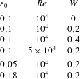
The actual values of the base flow parameters are chosen as listed in table 1. In order to study curvature instability, we consider thin vortex rings at high Reynolds numbers. We set the Reynolds number to
 $Re=10^{4}$
, while
 $Re=5\times 10^{4}$
is also used for comparison. The prescribed values of the thickness are
 $\unicode[STIX]{x1D700}_{0}=0.1$
and
 $0.18$
, while
 $\unicode[STIX]{x1D700}_{0}=0.05$
is also used for a limited number of cases. The swirl parameter is set to
 $W=0,0.2$
and
 $0.4$
as in Blanco-Rodríguez & Le Dizès (Reference Blanco-Rodríguez and Le Dizès2017); in this range of
 $W$
the swirl is sufficiently small that the swirling jet instability is not present. The range of wavenumber is set to
 $1\leqslant k\leqslant 4$
or
 $1\leqslant k\leqslant 4.5$
depending on the case.
Grid spacing in
 $r$
direction. Grid B.

Base flow parameters.

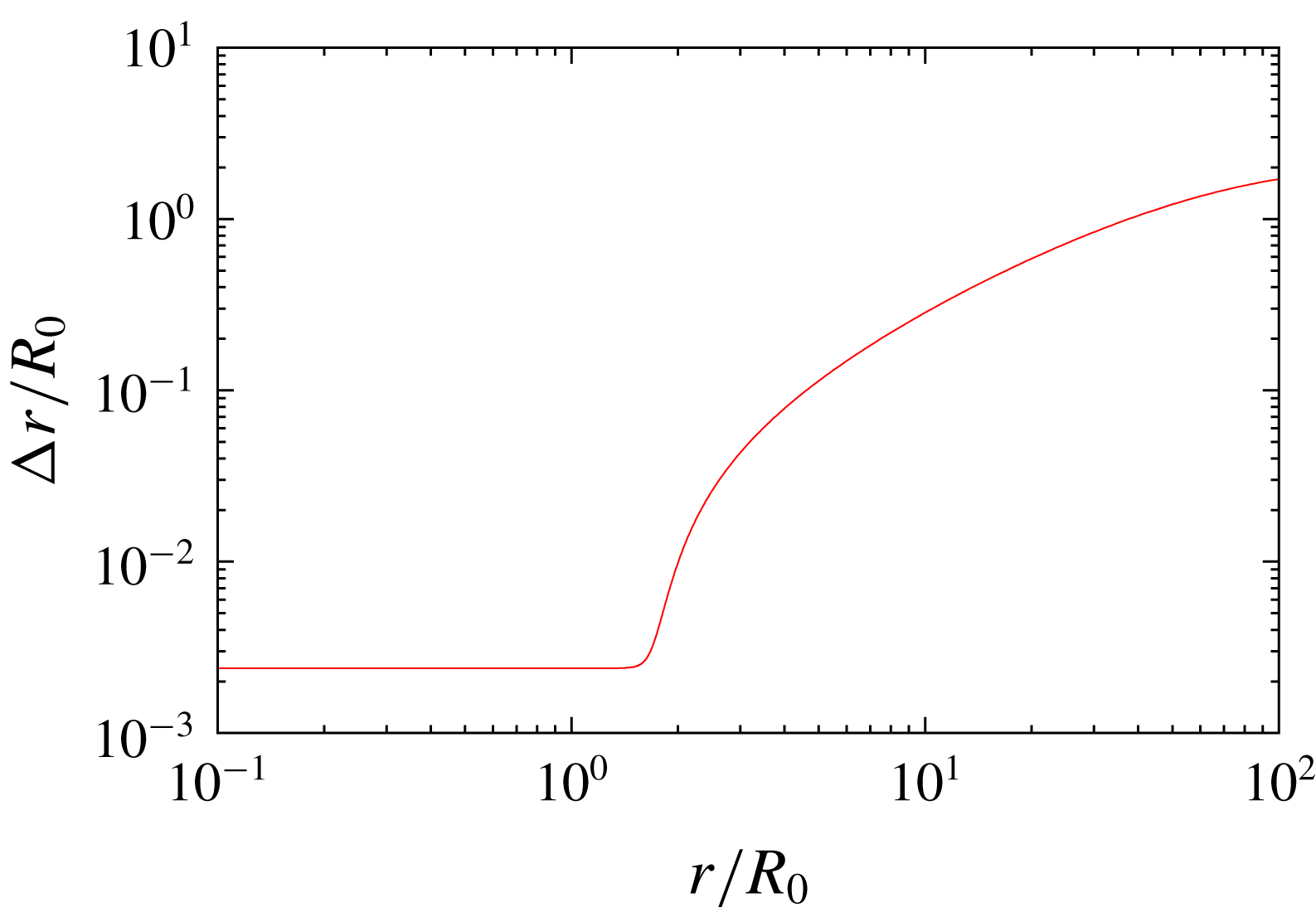
The radial size of the domain is set to
 $L_{r}=100R_{0}$
, where
 $R_{0}$
is the initial radius of the vortex ring. Slip boundary conditions are imposed at
 $r=L_{r}$
. Imposing slip boundary conditions is equivalent to placing virtual vortices called image vortices outside the domain (Saffman Reference Saffman1992). The strength and the radial position of the image vortices become weaker and farther, respectively, as
 $L_{r}$
increases. Therefore, the outer boundary is set sufficiently far to make the effect of the image vortices negligible; see appendix B for dependence on
 $L_{r}$
. This large value of
 $L_{r}$
does not lead to a large number of grid points since non-uniform stretched grids are used in the
 $r$
direction (figure 2); the grid size at
 $r=L_{r}$
is
 $\unicode[STIX]{x0394}r=2R_{0}$
. The axial size of the domain is set to
 $L_{z}=4\unicode[STIX]{x03C0}/3R_{0}$
with periodic boundary conditions. This means that we actually simulate a row of vortex rings. However, for this value of
 $L_{z}$
, the effect of distant rings remains small compared to the self-induced effect of the ring on itself. The grid parameters are listed in table 2. The minimum grid size
 $\unicode[STIX]{x0394}r_{min}$
in the
 $r$
direction and the uniform grid spacing
 $\unicode[STIX]{x0394}z$
in the
 $z$
direction should be small enough to resolve waves on the vortex core; for
 $Re=10^{4}$
the minimum numbers of grid points within the diameter of the vortex core are
 $83$
and
 $98$
in the
 $r$
and
 $z$
directions, respectively, while the numbers of points are doubled for
 $Re=5\times 10^{4}$
since fine structures may appear as viscous diffusion becomes weak. We have confirmed that the grid resolution is sufficient (see appendix B). The time step
 $\unicode[STIX]{x0394}t$
is set proportional to the minimum grid size (table 2); for the dependence on the time step, also see appendix B, which shows that it is sufficiently small to give accurate results. The total time of integrating the linearized equations is
 $100$
–
 $200(R/u_{\unicode[STIX]{x1D719},max})$
, for which the error of the growth rate of a curvature instability mode is less than
 $0.01\,\%$
.
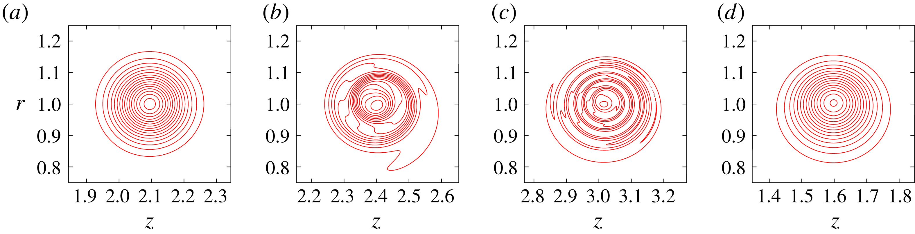
Time evolution of a vortex ring. Contours of
 $v$
. Here
 $Re=10^{4},\unicode[STIX]{x1D700}=0.1,W=0.2$
;
 $t=0,1,3,12$
. Contour levels are
 $v/W=0.0638n$
(
 $n=1,2,\ldots$
).

Grid parameters.

3 Base flow
In this section we show how we obtain the quasi-steady state of the vortex ring that is used as a base flow. Starting from Gaussian distributions of azimuthal vorticity and swirl velocity (figure 3), the vortex ring reaches a quasi-steady state after a certain time of evolution. There are subtle issues concerning controlling parameters
 $\unicode[STIX]{x1D700}$
and
 $W$
since they both evolve in time; how we control them is also explained.
Figure 3 shows the time evolution of a vortex ring by contours of
 $v$
for
 $Re=10^{4}$
,
 $W=0.2$
. After transient evolution (figure 3
b,c) the vortex ring reaches a quasi-steady state by
 $t=12$
(figure 3
d). For an exact steady state of inviscid axisymmetric flow
 $\unicode[STIX]{x1D714}_{\unicode[STIX]{x1D703}}/r$
becomes a function of the Stokes streamfunction
 $\unicode[STIX]{x1D6F9}$
when
 $W=0$
, while
 $rv$
becomes a function of
 $\unicode[STIX]{x1D6F9}$
when
 $W\neq 0$
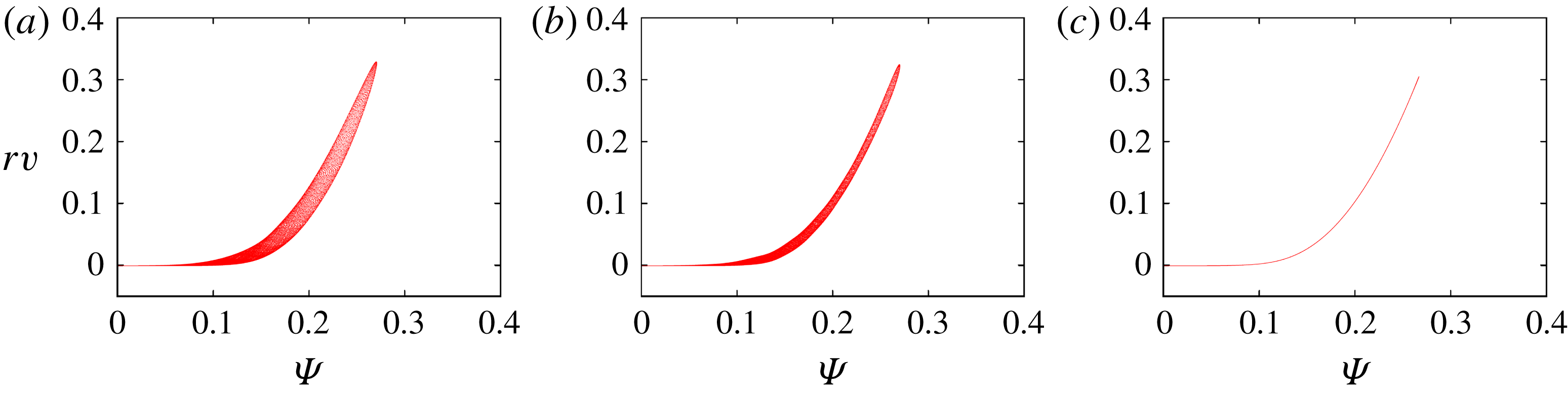
. This is confirmed in figure 4 which shows scatter plots of
 $\unicode[STIX]{x1D6F9}$
and
 $rv$
. The thickness of the scatter plot becomes small as time proceeds; at
 $t=12$
we obtain a good functional relation between
 $\unicode[STIX]{x1D6F9}$
and
 $rv$
. We also confirmed a functional relation between
 $\unicode[STIX]{x1D6F9}$
and
 $\unicode[STIX]{x1D714}_{\unicode[STIX]{x1D703}}/r$
for
 $W=0$
, but this result is not shown here since it is well documented in previous works (Shariff et al.
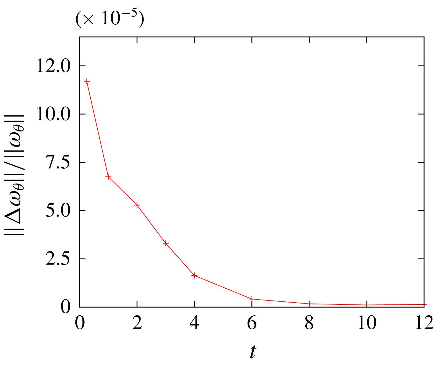
Reference Shariff, Verzicco and Orlandi1994). Quasi-steadiness is also checked by the
 $L^{2}$
-norm of
 $$\begin{eqnarray}\displaystyle \unicode[STIX]{x0394}\unicode[STIX]{x1D714}_{\unicode[STIX]{x1D703}}=\unicode[STIX]{x1D714}_{\unicode[STIX]{x1D703}}(t+\unicode[STIX]{x0394}t,r,z+U\unicode[STIX]{x0394}t)-\unicode[STIX]{x1D714}_{\unicode[STIX]{x1D703}}(t,r,z), & & \displaystyle\end{eqnarray}$$
which is the difference of the azimuthal vorticity between two adjacent time steps (figure 5); here
 $U$
is the translating velocity (figure 6
b). It is observed that the difference decreases as time proceeds and becomes close to zero after
 $t\approx 10$
.
Scatter plot of
 $\unicode[STIX]{x1D6F9}$
and
 $rv$
. Here
 $Re=10^{4},\unicode[STIX]{x1D700}=0.1,W=0.2$
;
 $t=1,3,12$
.

The
 $L^{2}$
-norm of
 $\unicode[STIX]{x0394}\unicode[STIX]{x1D714}_{\unicode[STIX]{x1D703}}=\unicode[STIX]{x1D714}_{\unicode[STIX]{x1D703}}(t+\unicode[STIX]{x0394}t,r,z+U\unicode[STIX]{x0394}t)-\unicode[STIX]{x1D714}_{\unicode[STIX]{x1D703}}(t,r,z)$
. Here
 $Re=10^{4},\unicode[STIX]{x1D700}=0.1,W=0.2$
.

Time evolution of (a) squared core radius and (b) translating velocity. Here
 $Re=10^{4},\unicode[STIX]{x1D700}=0.1,W=0,0.2,0.4$
. The slope of the dot-dashed line in (a) is
 $4\unicode[STIX]{x1D708}$
.

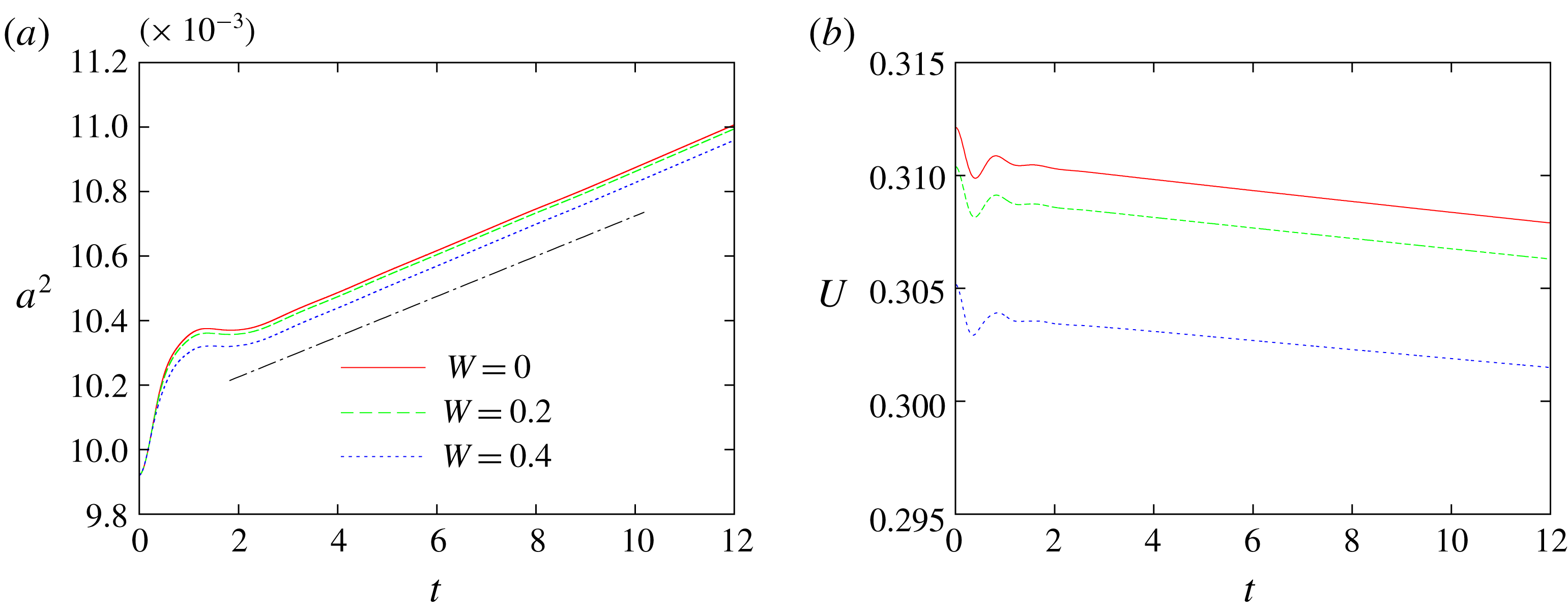
Figure 6 shows the time evolution of squared core radius and translating velocity of a vortex ring. The vortex core spreads due to viscous diffusion as
 $$\begin{eqnarray}\displaystyle a^{2}(t)=a_{0}^{2}+4\unicode[STIX]{x1D708}t & & \displaystyle\end{eqnarray}$$
after a transient behaviour which depends on the initial conditions (initial transient). The increase of the core radius affects resonance condition of curvature and elliptic instabilities since the wavenumber non-dimensionalized by the core radius determines the condition. This figure also shows the effects of swirl: both the core radius and translating velocity decrease slightly for larger swirl. The latter result is in agreement with analytical results (Widnall, Bliss & Zalay Reference Widnall, Bliss, Zalay, Olsen, Goldburg and Rogers1971).
Time evolution of swirl parameter: (a)
 $W$
and (b)
 $Wa$
. Here
 $Re=10^{4},5\times 10^{4}$
,
 $W\approx 0.2$
.

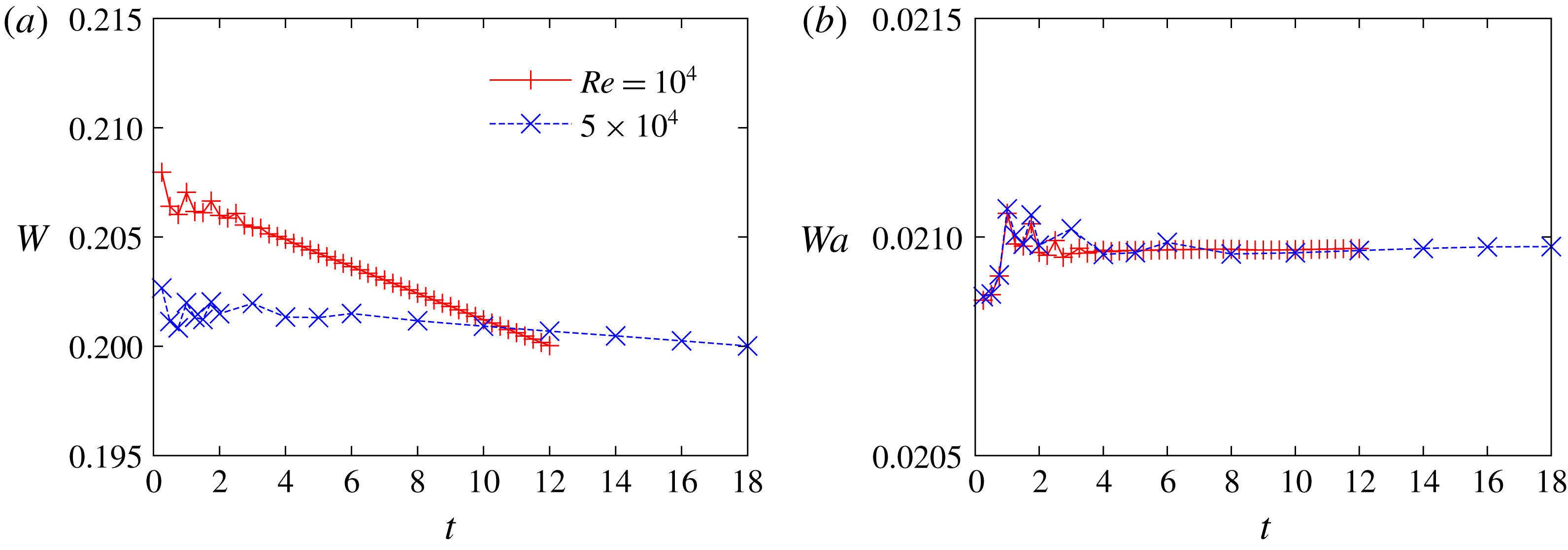
Figure 7 shows time evolution of the swirl parameter
 $W=0.638v_{max}/u_{\unicode[STIX]{x1D719},max}$
. The swirl velocity decreases monotonically after an initial transient. This result is explained as follows. Since the angular momentum
 $A_{z}\approx v_{max}\unicode[STIX]{x03C0}a^{2}R$
is approximately constant, we have
 $$\begin{eqnarray}\displaystyle v_{max}\propto \frac{1}{a^{2}} & & \displaystyle\end{eqnarray}$$
when the ring radius is nearly constant. On the other hand, since the circulation is also approximately constant, we have
 $$\begin{eqnarray}\displaystyle u_{\unicode[STIX]{x1D719},max}\propto \frac{\unicode[STIX]{x1D6E4}}{2\unicode[STIX]{x03C0}a}. & & \displaystyle\end{eqnarray}$$
Therefore, the ratio decreases with time as
 $W\propto a^{-1}$
, which is confirmed in figure 7(b). The initial values of the core radius and the swirl parameter are determined taking account of their time evolutions so that they become prescribed values when the flow becomes quasi-steady. The results shown below are based on the quasi-steady states at
 $t=12$
and
 $18$
for
 $Re=10^{4}$
and
 $5\times 10^{4}$
, respectively.
4 Results
In this section we show linear stability results. First, the overall features of the linear instability are shown by growth rate and oscillation frequency plotted against azimuthal wavenumber; mode structures are identified for some typical unstable modes. Next, we focus on two curvature instability modes to make comparison between numerical and theoretical results. Finally, other modes of interest are shown and discussed.
4.1 Growth rate
The unstable modes obtained at large
 $t$
are proportional to
 $\text{e}^{(\unicode[STIX]{x1D70E}+\text{i}\unicode[STIX]{x1D714})t}$
. The growth rate
 $\unicode[STIX]{x1D70E}$
and oscillation frequency
 $\unicode[STIX]{x1D714}$
are shown as a function of the azimuthal wavenumber
 $k$
in figures 8–11. The Reynolds number is fixed at
 $10^{4}$
. The thickness
 $\unicode[STIX]{x1D700}$
is approximately
 $0.1$
in figures 8–10 and
 $0.18$
in figure 11. The swirl parameter
 $W$
is
 $0$
,
 $0.2$
and
 $0.4$
in figures 8, 9 and 10, respectively, while it is also set to
 $0.2$
in figure 11.
Several peaks of the growth rate are observed in each case; the width of the peaks is narrow for
 $\unicode[STIX]{x1D700}_{0}=0.1$
as the instability is mostly due to parametric resonance and it becomes wide for
 $\unicode[STIX]{x1D700}_{0}=0.18$
as the width is essentially proportional to
 $\unicode[STIX]{x1D700}_{0}$
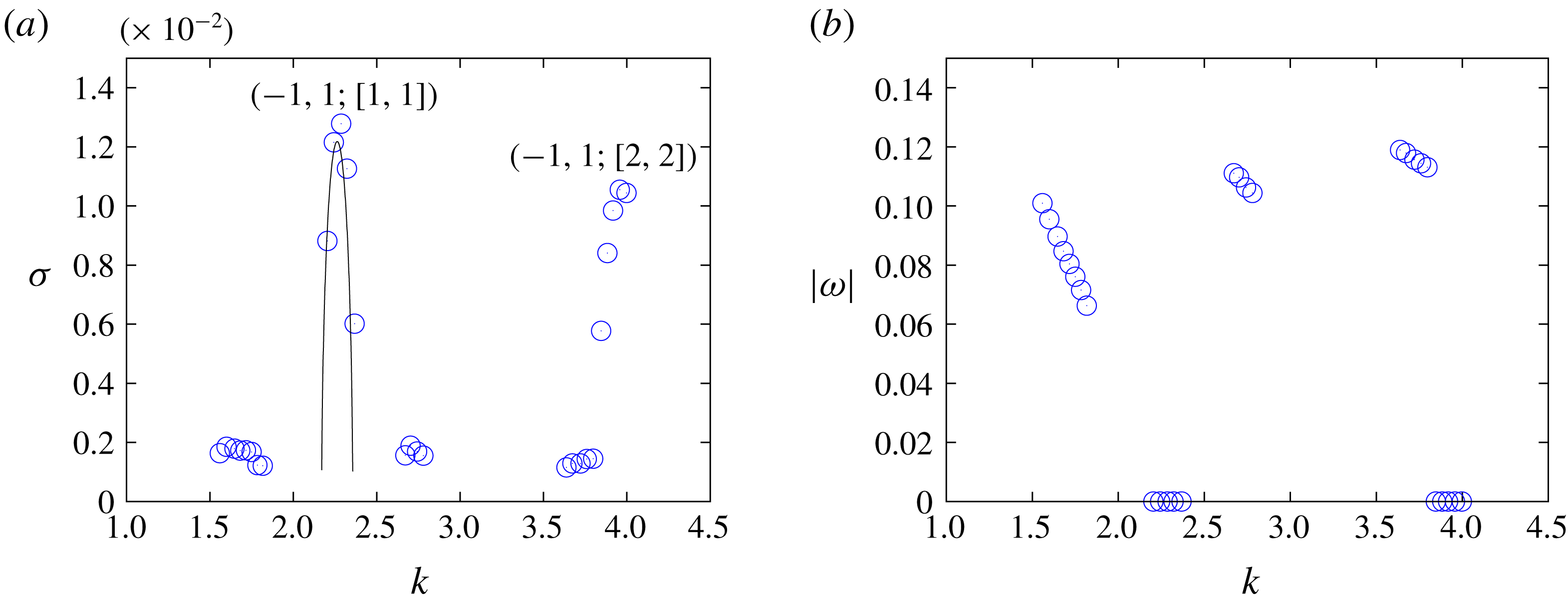
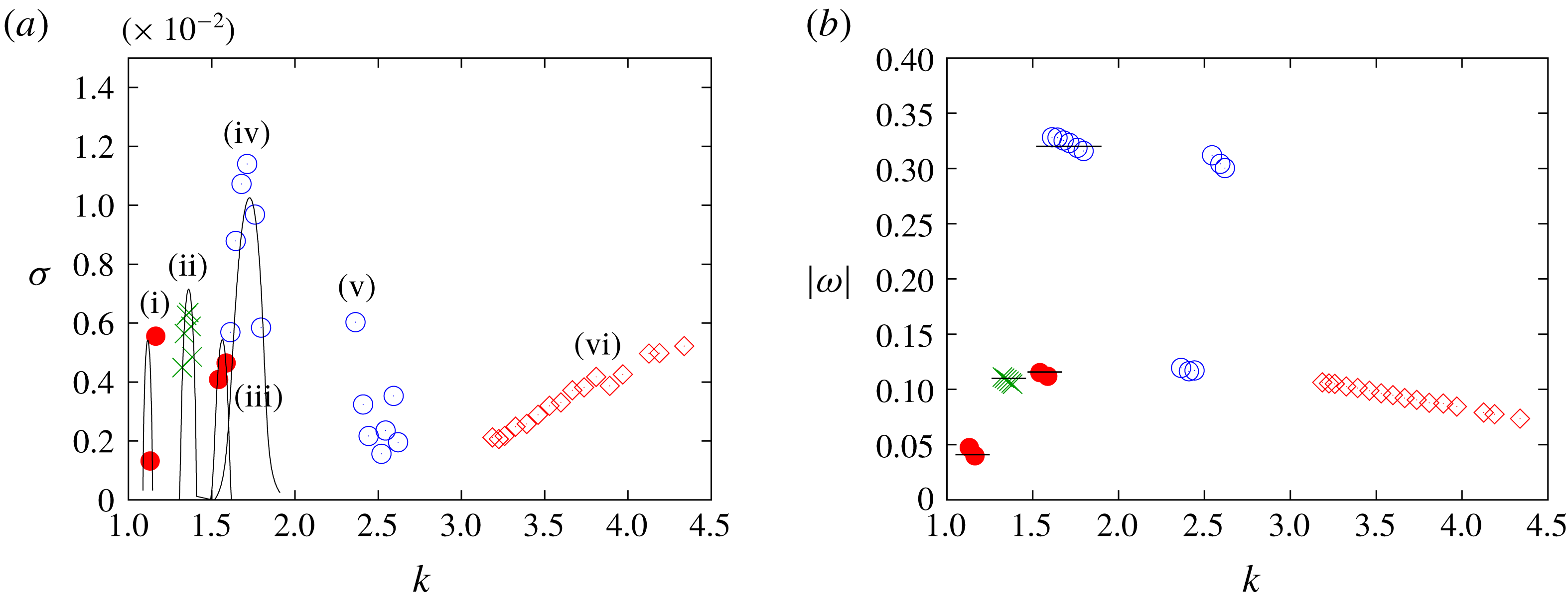
. In these figures typical modes are identified by their structures. The instability is due to either the curvature instability (marked by filled circles and crosses) or the elliptic instability (marked by open circles) except for the spiral modes (marked by diamonds for
 $W=0.4$
). Most of the modes are composed of two inertial waves which are indexed by the branch of dispersion curves. For example, the most unstable mode for
 $\unicode[STIX]{x1D700}_{0}=0.1$
and
 $W=0$
(figure 8) is due to elliptic instability and consists of the
 $m=\pm 1$
inertial waves of the first branches which crosses at
 $(k,\unicode[STIX]{x1D714})=(2.333,0)$
so that it is labelled as
 $(-1,1;[1,1])$
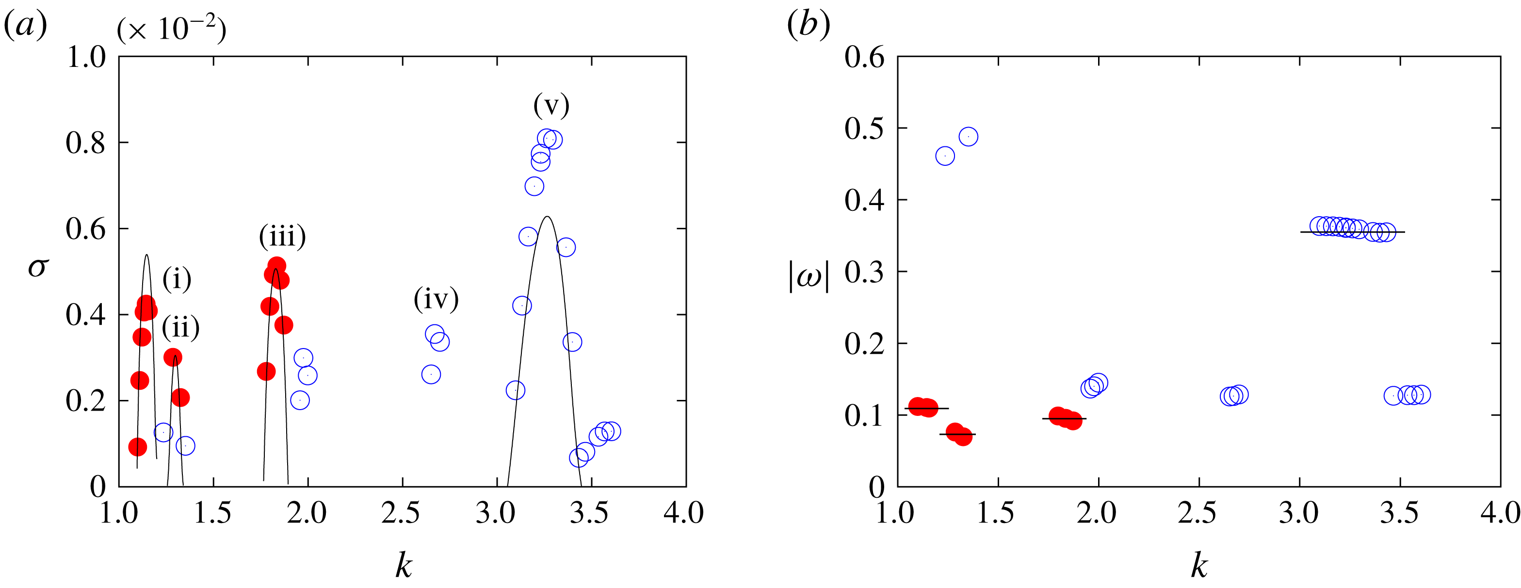
. The mode labelled by (i) for
 $\unicode[STIX]{x1D700}_{0}=0.1$
and
 $W=0.2$
(figure 9) is due to curvature instability and consists of the
 $m=-1$
inertial wave of the first branch and the
 $m=0$
inertial wave of the third branch, which crosses at
 $(k,\unicode[STIX]{x1D714})=(1.14,-0.11)$
, so that it is denoted as
 $(-1,0;[1,3])$
. It is pointed out that the sign of
 $m$
and thereby the order of the indices of the branches are different from Blanco-Rodríguez & Le Dizès (Reference Blanco-Rodríguez and Le Dizès2017) since we choose
 $k$
to be positive in the present work:
 $(-1,0;[1,3])$
with
 $(k,\unicode[STIX]{x1D714})=(1.14,-0.11)$
in the present work corresponds to
 $(m_{A},m_{B})=(0,1)$
and
 $(l_{A},l_{B})=(3,1)$
with
 $(k,\unicode[STIX]{x1D714})=(-1.14,0.11)$
in Blanco-Rodríguez & Le Dizès (Reference Blanco-Rodríguez and Le Dizès2017). Theoretical values for some typical modes taken from Blanco-Rodríguez & Le Dizès (Reference Blanco-Rodríguez and Le Dizès2016) and Blanco-Rodríguez & Le Dizès (Reference Blanco-Rodríguez and Le Dizès2017) are also included by lines in figures 8–11.
(a) Growth rate (
 $\unicode[STIX]{x1D70E}=\text{Im}(\unicode[STIX]{x1D714})$
) and (b) frequency (
 $\text{Re}(\unicode[STIX]{x1D714})$
) plotted against azimuthal wavenumber. Here
 $\unicode[STIX]{x1D700}_{0}=0.1$
,
 $Re=10^{4},W=0$
. All modes are due to elliptic instability marked by open circles. The lines show theoretical values (Blanco-Rodríguez & Le Dizès Reference Blanco-Rodríguez and Le Dizès2016).

(a) Growth rate and (b) frequency plotted against azimuthal wavenumber. Here
 $\unicode[STIX]{x1D700}_{0}=0.1$
,
 $Re=10^{4},W=0.2$
. Filled circles: curvature instability; open circles: elliptic instability. The lines show theoretical values (Blanco-Rodríguez & Le Dizès Reference Blanco-Rodríguez and Le Dizès2016, Reference Blanco-Rodríguez and Le Dizès2017). Some typical modes are identified: (i)
 $(-1,0;[1,3])$
, (ii)
 $(-1,0;[1,4])$
, (iii)
 $(-1,0;[2,4])$
, (iv)
 $(-1,1;[2,1])$
, (v)
 $(-2,0;[2,2])$
.

(a) Growth rate and (b) frequency plotted against azimuthal wavenumber. here
 $\unicode[STIX]{x1D700}_{0}=0.1$
,
 $Re=10^{4},W=0.4$
. The symbols and lines are the same as in figure 9, while the crosses and the diamonds correspond to three-wave modes and spiral modes, respectively. Modes are (i)
 $(-1,0;[1,3])$
, (ii) three-wave mode, (iii)
 $(-1,0;[3,2])$
, (iv)
 $(-2,0;[1,1])$
, (v)
 $(-2,0;[1,2])$
, (vi) spiral mode.

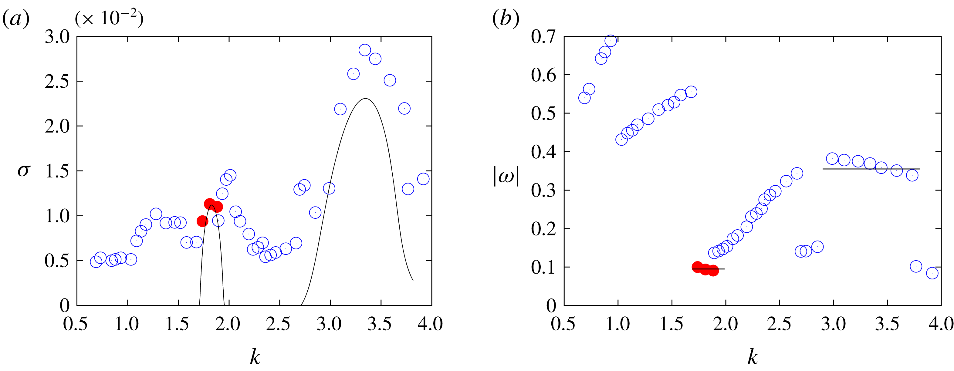
(a) Growth rate and (b) frequency plotted against azimuthal wavenumber. Here
 $\unicode[STIX]{x1D700}_{0}=0.18$
,
 $Re=10^{4},W=0.2$
. The symbols and lines are the same as in figure 9.

For
 $\unicode[STIX]{x1D700}_{0}=0.1$
and
 $W=0$
(figure 8) the instability is due to elliptic instability. The growth rate of curvature instability for
 $W=0$
is too small to be the most unstable mode or be captured by numerical simulation. Two modes have large growth rates; the indices of the branches of the two waves are the same and they are often called principal modes. The frequency is zero for these modes. The values of the growth rate are in good agreement with theory. There are also modes with small growth rate and non-zero frequency; the indices of the two inertial waves are different for these modes.
For
 $\unicode[STIX]{x1D700}_{0}=0.1$
and
 $W=0.2$
(figure 9) three modes of curvature instability are identified: (i)
 $(-1,0;[1,3])$
, (ii)
 $(-1,0;[1,4])$
and (iii)
 $(-1,0;[2,4])$
. The other modes are due to elliptic instability; two modes are identified: (iv)
 $(-1,1;[2,1])$
and (v)
 $(-2,0;[2,2])$
. They are also found in previous works for a strained vortex and a vortex pair (Lacaze, Ryan & Le Dizès Reference Lacaze, Ryan and Le Dizès2007; Roy et al.
Reference Roy, Schaeffer, Le Dizès and Thompson2008). It is known that asymmetric modes like
 $(-2,0;[2,2])$
have large growth rate when the swirl is added. In the present range of wavenumber
 $1\leqslant k\leqslant 4$
, the most unstable mode is the elliptic instability of
 $(-2,0;[2,2])$
, while the second most unstable mode is the curvature instability of
 $(-1,0;[2,4])$
. All modes are oscillatory having non-zero frequencies. The values of the growth rate are in good agreement for the curvature instability of
 $(-1,0;[2,4])$
, while some differences are observed for the elliptic instability of
 $(-2,0;[2,2])$
and the curvature instability of
 $(-1,0;[1,3])$
. The growth rate of the curvature instability modes will be compared carefully to theory in the next subsection.
For
 $\unicode[STIX]{x1D700}_{0}=0.1$
and
 $W=0.4$
(figure 10) three modes of curvature instability are identified: (i)
 $(-1,0;[1,3])$
, (ii) three-wave mode and (iii)
 $(-1,0;[3,2])$
. The structure of the three-wave mode is detailed later in § 4.3.2. Three modes of elliptic instability are also observed. Two modes having larger growth rate are identified: (iv)
 $(-2,0;[1,1])$
and (v)
 $(-2,0;[2,1])$
(see also figure 22
b). Again these modes are also found in previous works (Lacaze et al.
Reference Lacaze, Ryan and Le Dizès2007; Roy et al.
Reference Roy, Schaeffer, Le Dizès and Thompson2008). The spiral mode is different from the other modes in that its growth rate does not have a clear peak; it extends in the wavenumber range
 $3.2\leqslant k$
. The structure of this mode is discussed in § 4.3.3.
We show the case
 $\unicode[STIX]{x1D700}_{0}=0.18$
and
 $W=0.2$
in figure 11 to see the effects of the core size by comparing to figure 9. Only one mode of curvature instability
 $(-1,0;[2,4])$
survives as the growth rate of elliptic instability increases as
 $\unicode[STIX]{x1D700}^{2}$
which is faster than that of curvature instability
 $\unicode[STIX]{x1D700}$
. The band width of each mode broadens as is observed for the most unstable mode at
 $k\approx 3.4$
due to elliptic instability. As a result the vortex ring is unstable at any wavenumber
 $k$
in the present range.
4.2 Typical curvature instability modes and critical layer damping
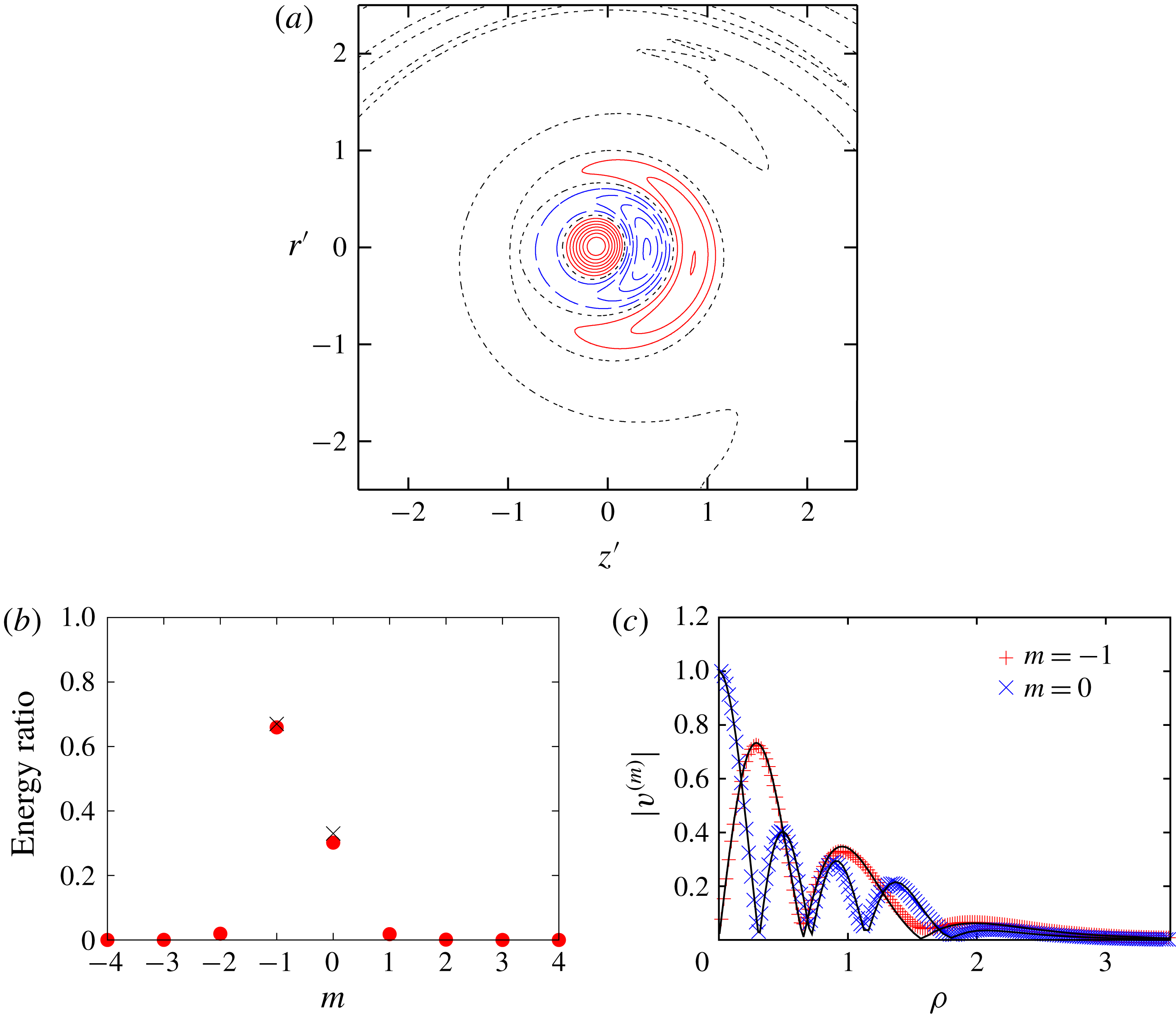
Mode structure. The
 $(-1,0;[2,4])$
mode with
 $(k,\unicode[STIX]{x1D714})=(1.853,-0.095)$
. Here
 $W=0.2$
,
 $Re=10^{4}$
,
 $\unicode[STIX]{x1D700}_{0}=0.1$
. (a) Contours of azimuthal component of vorticity
 $\unicode[STIX]{x1D714}_{\unicode[STIX]{x1D703}}$
:
 $\unicode[STIX]{x1D714}_{\unicode[STIX]{x1D703}}>0$
(solid),
 $\unicode[STIX]{x1D714}_{\unicode[STIX]{x1D703}}=0$
(dotted) and
 $\unicode[STIX]{x1D714}_{\unicode[STIX]{x1D703}}<0$
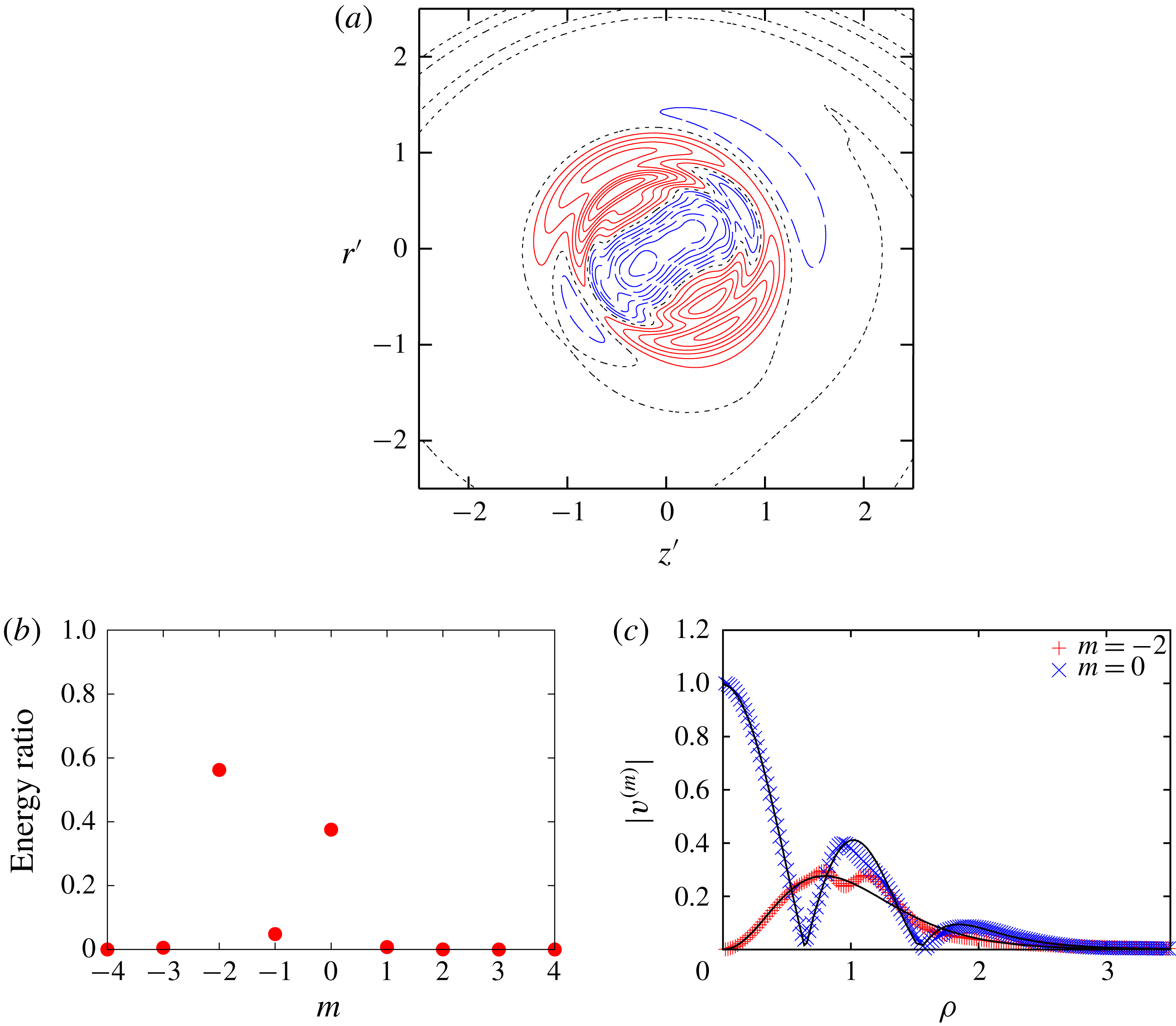
(dashed). (b) Ratio of energy; filled circles: DNS; crosses: theory. (c) Radial distribution of
 $v^{(m)}$
; symbols: DNS; lines: theory.

Next, we focus on the two modes of curvature instability for
 $W=0.2$
:
 $(-1,0;[1,3])$
and
 $(-1,0;[2,4])$
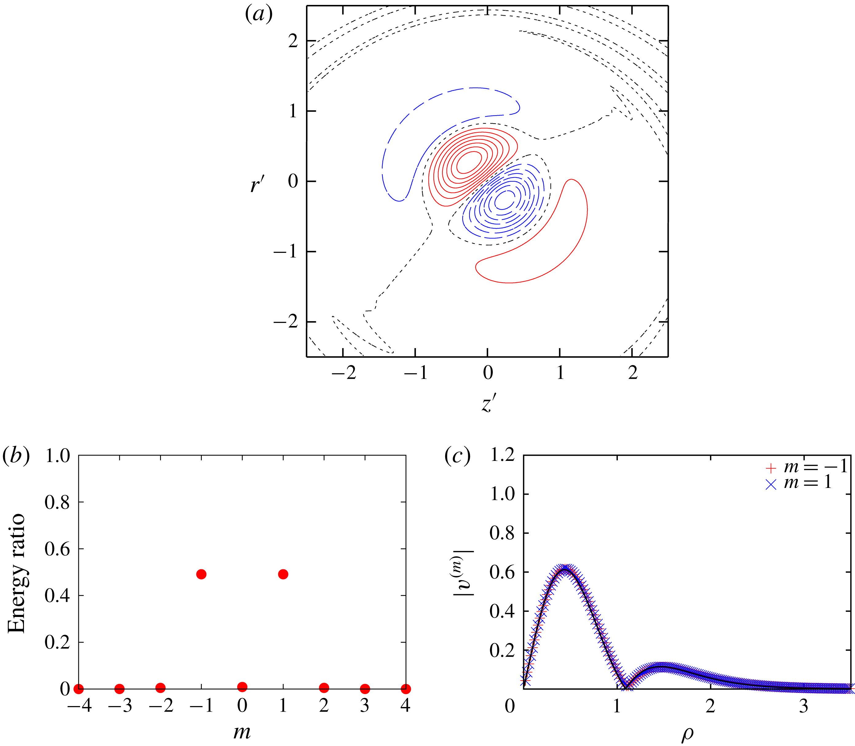
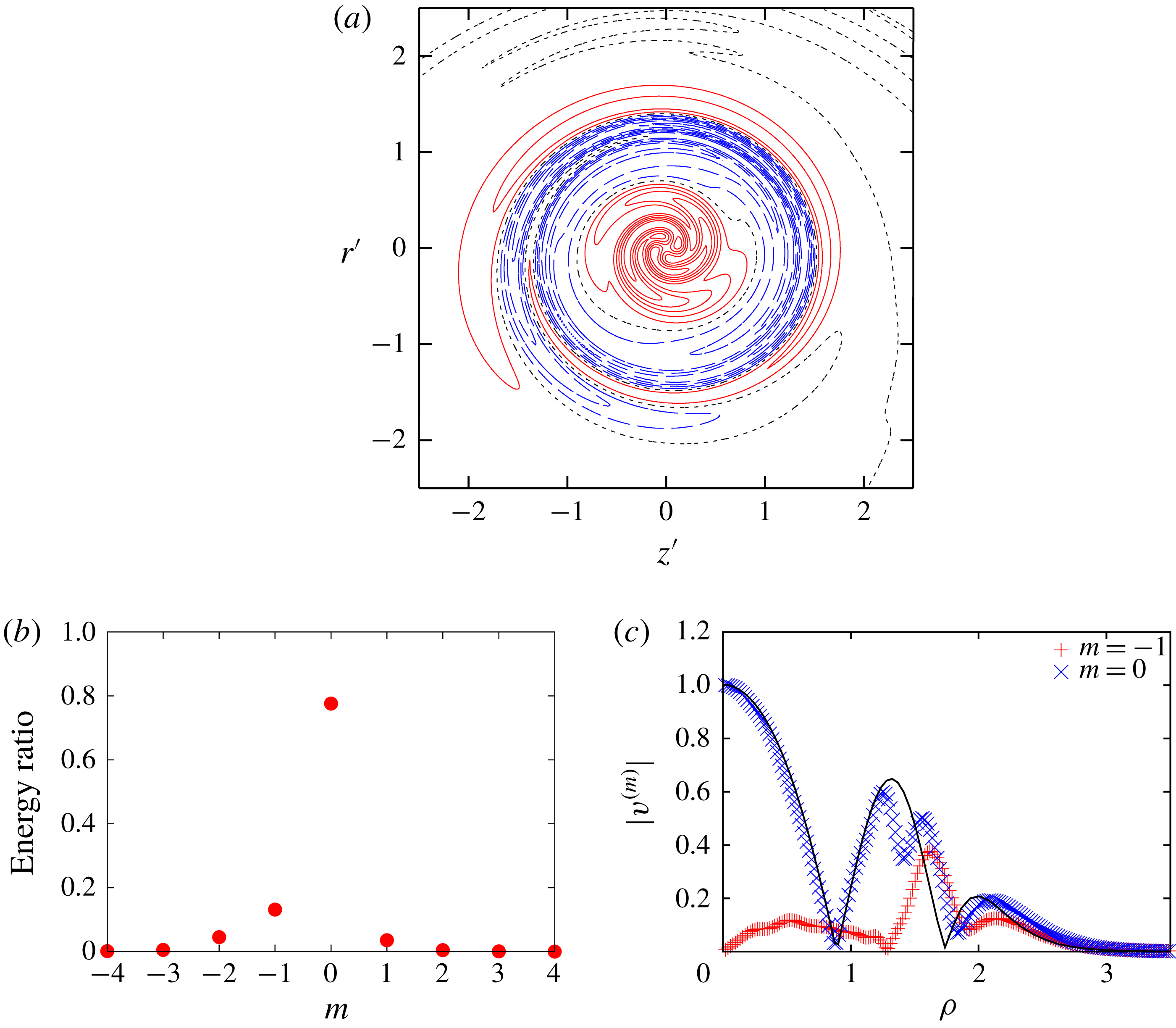
. Figure 12 shows the structure of the curvature instability mode
 $(-1,0;[2,4])$
. Contours of azimuthal vorticity
 $\unicode[STIX]{x1D714}_{\unicode[STIX]{x1D703}}$
are shown in figure 12(a). This figure is similar to figure 7(e) in Blanco-Rodríguez & Le Dizès (Reference Blanco-Rodríguez and Le Dizès2017). In order to reveal the mode structure, we decompose the unstable mode as
 $$\begin{eqnarray}\displaystyle \hat{\boldsymbol{u}}(r,z)=\mathop{\sum }_{m}\boldsymbol{u}^{(m)}(\unicode[STIX]{x1D70C})\text{e}^{\text{i}m\unicode[STIX]{x1D719}}, & & \displaystyle\end{eqnarray}$$
where
 $(\unicode[STIX]{x1D70C},\unicode[STIX]{x1D719})$
is the local polar coordinate system of which origin is the centre of the vortex core of the base flow in the
 $rz$
-plane (figure 1). In figure 12(b) the ratio of energy is plotted against
 $m$
. It shows that this mode consists of
 $m=-1$
and
 $m=0$
waves and the values are in good agreement with theory. The structure of each wave is shown by the radial distribution of the azimuthal component of the velocity field
 $v$
in figure 12(c). The number of points where the magnitude of the wave vanishes (
 $r=0$
excluded) coincides with the index of the branch; in the present case the
 $m=-1$
wave has two zeros, while the
 $m=0$
wave has four zeros. Thus the mode is labelled as
 $(-1,0;[2,4])$
. Theoretical results are also shown in figure 12(c); they are in excellent agreement with the numerical results.
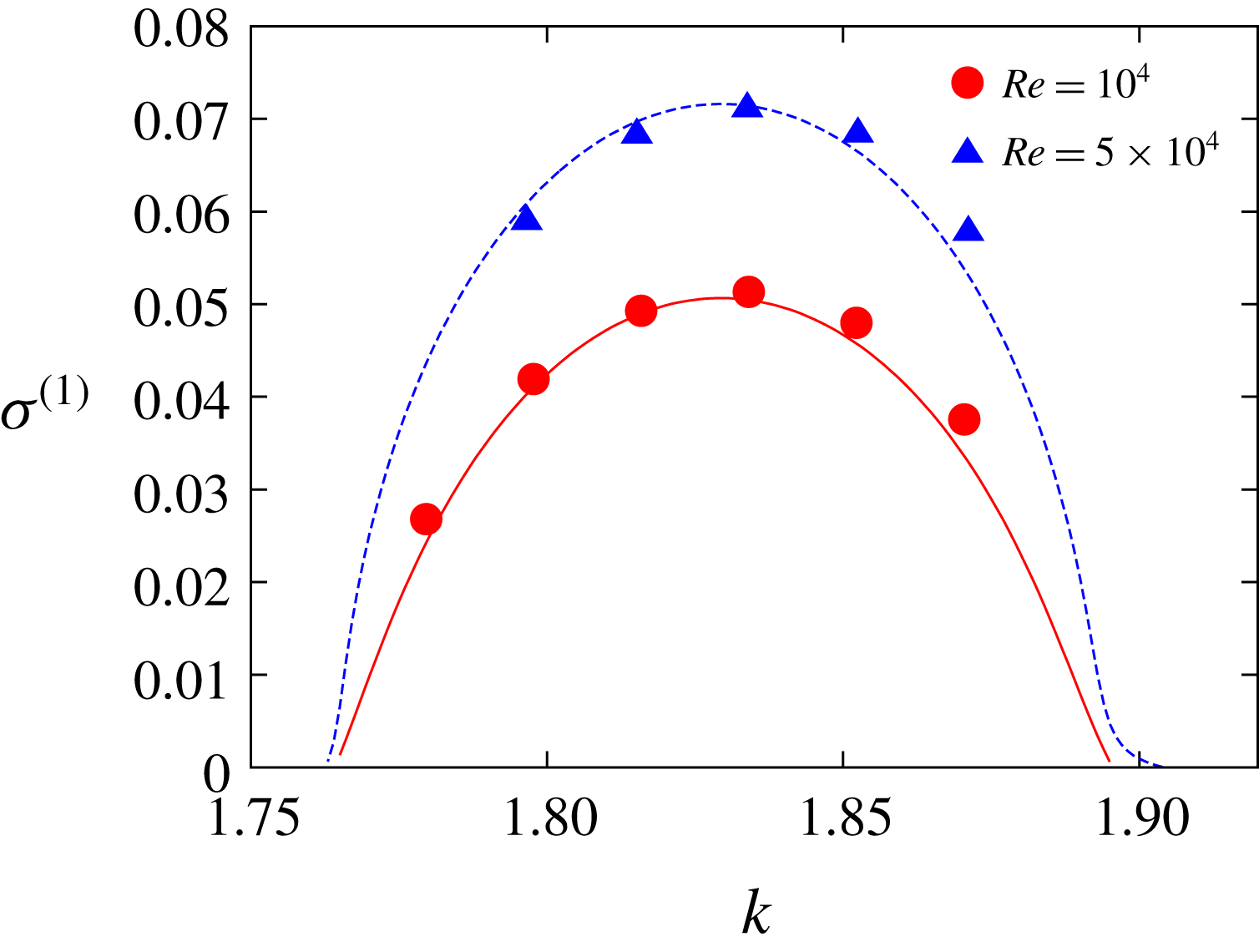
Growth rates. Here
 $W=0.2$
,
 $(-1,0;[2,4])$
mode,
 $\unicode[STIX]{x1D700}_{0}=0.1$
,
 $Re=10^{4},5\times 10^{4}$
. Symbols: DNS; lines: theory.

Figure 13 compares the growth rate with theory (Blanco-Rodríguez & Le Dizès Reference Blanco-Rodríguez and Le Dizès2017) for the curvature instability mode
 $(-1,0;[2,4])$
. In this figure the growth rate is divided by
 $\unicode[STIX]{x1D700}$
:
 $\unicode[STIX]{x1D70E}^{(1)}=\unicode[STIX]{x1D70E}/\unicode[STIX]{x1D700}$
. They are also in good agreement having approximately the same maximum and band width. It is pointed out that the critical layer damping is small for this mode (Blanco-Rodríguez & Le Dizès Reference Blanco-Rodríguez and Le Dizès2017).
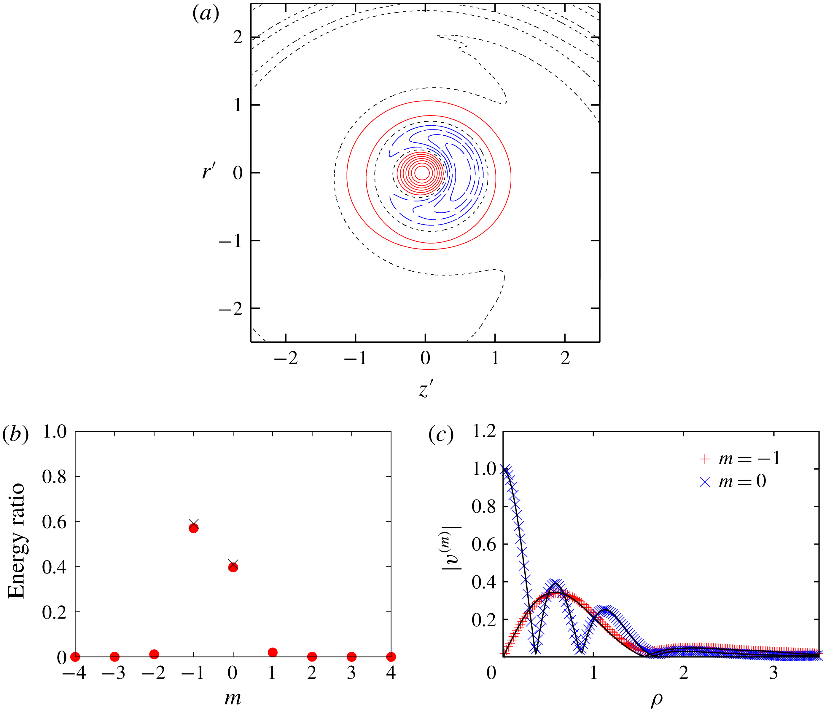
Mode structure. The
 $(-1,0;[1,3])$
mode with
 $(k,\unicode[STIX]{x1D714})=(1.144,-0.110)$
. Here
 $W=0.2$
,
 $Re=10^{4}$
,
 $\unicode[STIX]{x1D700}_{0}=0.1$
. (a) Contours of azimuthal component of vorticity
 $\unicode[STIX]{x1D714}_{\unicode[STIX]{x1D703}}$
:
 $\unicode[STIX]{x1D714}_{\unicode[STIX]{x1D703}}>0$
(solid),
 $\unicode[STIX]{x1D714}_{\unicode[STIX]{x1D703}}=0$
(dotted) and
 $\unicode[STIX]{x1D714}_{\unicode[STIX]{x1D703}}<0$
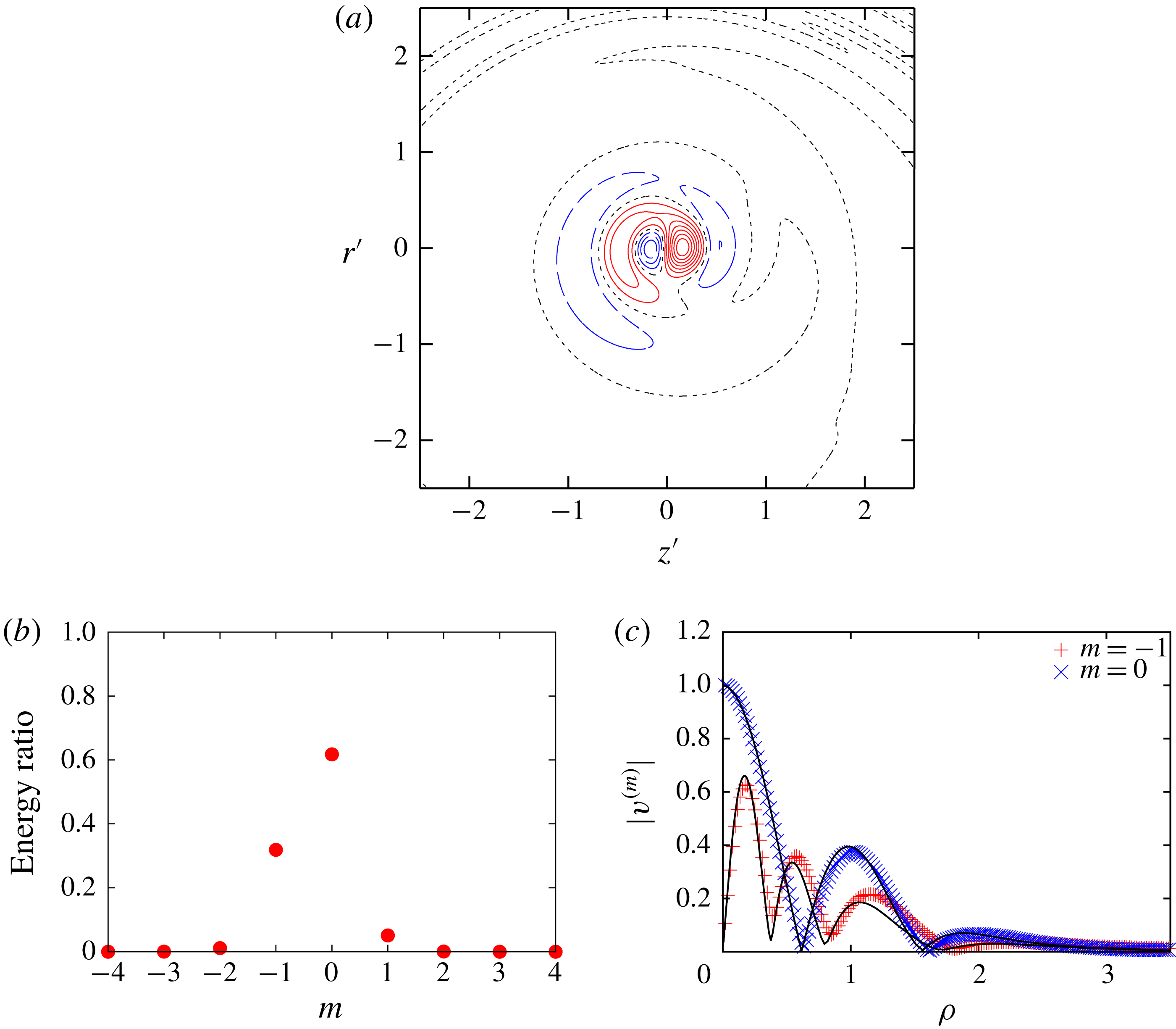
(dashed). (b) Ratio of energy; filled circles: DNS; crosses: theory. (c) Radial distribution of
 $v^{(m)}$
; symbols: DNS; lines: theory.

Figure 14 shows the structure of the curvature instability mode
 $(-1,0;[1,3])$
. Again the vorticity distribution is similar to the theoretical results (Blanco-Rodríguez & Le Dizès Reference Blanco-Rodríguez and Le Dizès2017). This mode consists of the
 $m=-1$
inertial wave of the first branch and the
 $m=0$
inertial wave of the third branch (figure 14
b,c). The radial distributions are in good agreement between the theoretical and numerical results (figure 14
c).
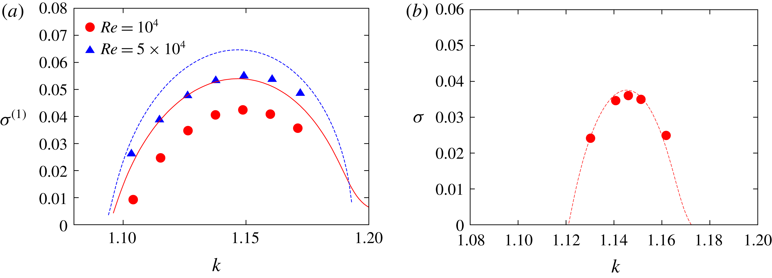
Growth rates. Here
 $W=0.2$
,
 $(-1,0;[1,3])$
mode. (a)
 $\unicode[STIX]{x1D700}_{0}=0.1$
,
 $Re=10^{4},5\times 10^{4}$
, (b)
 $\unicode[STIX]{x1D700}_{0}=0.05$
,
 $Re=10^{4}$
. Symbols: DNS; lines: theory.

Figure 15(a) compares the growth rate with theory (Blanco-Rodríguez & Le Dizès Reference Blanco-Rodríguez and Le Dizès2017) for the curvature instability mode
 $(-1,0;[1,3])$
. In contrast to figure 13 for the mode
 $(-1,0;[2,4])$
, the numerical results are smaller than the theoretical values for
 $\unicode[STIX]{x1D700}_{0}=0.1$
; the maximum growth rate is
 $\unicode[STIX]{x1D70E}^{(1)}=0.0424$
, which is
 $22\,\%$
smaller than the theoretical value
 $\unicode[STIX]{x1D70E}^{(1)}=0.0541$
; it is worth noting that the difference between the numerical and theoretical values does not depend on the Reynolds number very much. For
 $Re=5\times 10^{4}$
, the maximum growth rate is
 $\unicode[STIX]{x1D70E}^{(1)}=0.0549$
and the theoretical value is
 $\unicode[STIX]{x1D70E}^{(1)}=0.0646$
; the difference
 $0.0097$
for
 $Re=5\times 10^{4}$
is close to
 $0.0117$
for
 $Re=10^{4}$
. This suggests that the difference is not due to viscous diffusion. However, the difference becomes small for small core
 $\unicode[STIX]{x1D700}_{0}=0.05$
(figure 15
b). It is most likely that the difference for
 $\unicode[STIX]{x1D700}_{0}=0.1$
is due to the change in the critical layer damping as discussed below.
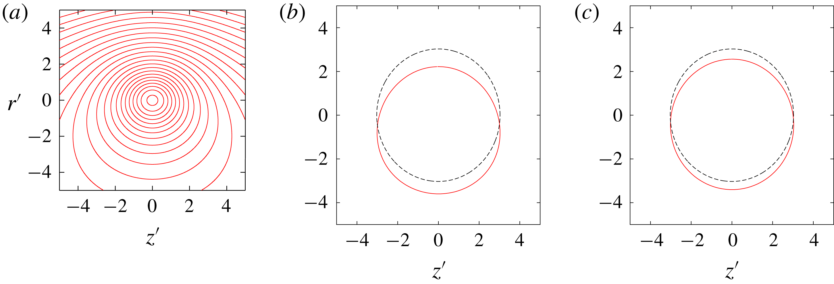
Theoretically, the critical layer damping is evaluated for the inertial waves on a straight axisymmetric vortex. However, the core of a vortex ring is deformed because of the curvature effects (figures 3 and 16
a); deformation is significant for larger
 $\unicode[STIX]{x1D700}$
. We resort to a heuristic argument to estimate the effect of deformation on the critical layer damping since rigorous analysis is difficult and beyond the scope of the present paper. It would be reasonable to approximate the critical layer on a deformed core by a streamline on which the averaged angular velocity
 $\overline{\unicode[STIX]{x1D6FA}}$
of a fluid particle satisfies an averaged version of equation (1.1)
 $$\begin{eqnarray}\displaystyle \unicode[STIX]{x1D714}-k\overline{u_{\unicode[STIX]{x1D719}}}-m\overline{\unicode[STIX]{x1D6FA}}=0. & & \displaystyle\end{eqnarray}$$
Figure 16(b,c) compares the approximated and theoretical critical layers for the
 $m=-1$
inertial wave of
 $(k,\unicode[STIX]{x1D714})=(1.14,-0.11)$
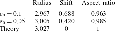
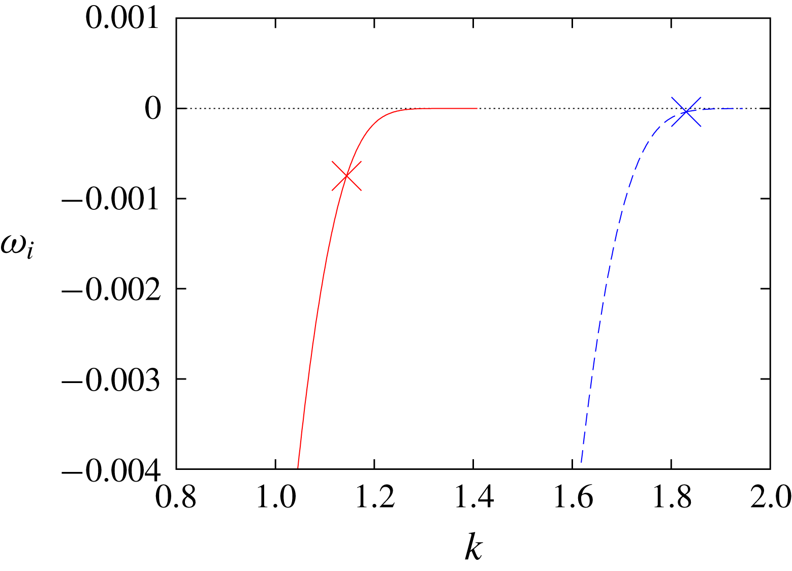
. The approximated critical layers are subjected to three types of deformation: they change in size (radius), shift downward and are elliptically deformed. Table 3 quantifies the deformation, where the elliptical deformation is measured by the aspect ratio which is the ratio of the short to long axis. On the other hand, the critical layer damping depends crucially on the position of the critical layer. Figure 17 shows the critical layer damping, which is the imaginary part of
 $\unicode[STIX]{x1D714}$
, plotted against the wavenumber
 $k$
for the first and second branches of the
 $m=-1$
inertial wave. The modes corresponding to the crossing points
 $(-1,0;[1,3])$
and
 $(-1,0;[2,4])$
are marked by symbols. A simple calculation shows that the theoretical growth rate almost agrees with the numerical value for
 $(-1,0;[1,3])$
if we replace the theoretical critical layer damping
 $-0.00075$
by
 $-0.003$
. This corresponds to
 $k=1.07$
in figure 17, which is
 $6.1\,\%$
smaller than
 $k=1.14$
at the crossing point. The deformation of the critical layer for
 $\unicode[STIX]{x1D700}_{0}=0.1$
is
 $2.0\,\%,23\,\%$
and
 $3.7\,\%$
in radius, shift and elliptical deformation, respectively. Therefore, the deformation of the critical layer can change the critical layer damping with the same order of magnitude observed in figure 15(a). Moreover, the change should be small for
 $\unicode[STIX]{x1D700}_{0}=0.05$
since deformation is small and it should be also small for
 $(-1,0;[2,4])$
since the critical layer damping for the mode
 $(-1,0;[2,4])$
is much smaller than that for
 $(-1,0;[1,3])$
as shown in figure 17. This heuristic argument explains why the difference between numerical and theoretical growth rates is large in figure 15(a), but not in figures 13 and 15(b), although it should be supported by more rigorous analysis.
(a) Streamlines of the base flow and (b,c) approximated (solid line) and theoretical (dashed line) positions of the critical layers of the inertial wave of
 $m=-1$
and
 $(k,\unicode[STIX]{x1D714})=(1.14,-0.11)$
,
 $Re=10^{4}$
,
 $W=0.2$
. (a,b)
 $\unicode[STIX]{x1D700}_{0}=0.1$
,
 $t=12$
, (c)
 $\unicode[STIX]{x1D700}_{0}=0.05$
,
 $t=16$
.

Deformation of critical layers.

Critical layer damping of the first and second branches. Here
 $W=0.2$
,
 $m=-1$
. Solid line: first branch; dashed line: second branch. The crosses correspond to the crossing points
 $(-1,0;[1,3])$
(
 $k=1.14$
on the first branch) and
 $(-1,0;[2,4])$
(
 $k=1.83$
on the second branch).

4.3 Other modes of interest
Here we focus on some other modes which are typical or interesting by showing the mode structures. The Reynolds number and the thickness are fixed to
 $10^{4}$
and
 $0.1$
, respectively.
4.3.1 Elliptic instability
Mode
 $(-1,1;[1,1]),k=2.333,\unicode[STIX]{x1D714}=0$
(elliptic instability). Here
 $W=0,Re=10^{4},\unicode[STIX]{x1D700}_{0}=0.1$
. (a) Contours of azimuthal component of vorticity
 $\unicode[STIX]{x1D714}_{\unicode[STIX]{x1D703}}:\,\unicode[STIX]{x1D714}_{\unicode[STIX]{x1D703}}\,>\,0$
(solid),
 $\unicode[STIX]{x1D714}_{\unicode[STIX]{x1D703}}=0$
(dotted) and
 $\unicode[STIX]{x1D714}_{\unicode[STIX]{x1D703}}<0$
(dashed). (b) Ratio of energy. (c) Radial distribution of
 $v^{(m)}$
; symbols: DNS; lines: theory.

Figure 18 shows the elliptic instability mode
 $(-1,1;[1,1])$
for
 $W=0$
. It is a well-known mode showing bending deformation in the direction of stretching due to the straining component of the base flow. The two inertial waves are symmetric: the energy ratio of each wave is
 $0.5$
(figure 18
b) and the radial distributions of the waves coincide (figure 18
c). The radial distributions are in excellent agreement between the theoretical and numerical results.
Mode
 $(-2,0;[1,2]),k=2.411,\unicode[STIX]{x1D714}=-0.119$
(elliptic instability). Here
 $W=0.4,Re=10^{4},\unicode[STIX]{x1D700}_{0}=0.1$
. (a) Contours of azimuthal component of vorticity
 $\unicode[STIX]{x1D714}_{\unicode[STIX]{x1D703}}$
:
 $\unicode[STIX]{x1D714}_{\unicode[STIX]{x1D703}}>0$
(solid),
 $\unicode[STIX]{x1D714}_{\unicode[STIX]{x1D703}}=0$
(dotted) and
 $\unicode[STIX]{x1D714}_{\unicode[STIX]{x1D703}}<0$
(dashed). (b) Ratio of energy. (c) Radial distribution of
 $v^{(m)}$
; symbols: DNS; lines: theory.

Figure 19 shows the elliptic instability mode
 $(-2,0;[1,2])$
for
 $W=0.4$
. The
 $m=-2$
wave of this mode has peaks near
 $\unicode[STIX]{x1D70C}\approx a$
, where the radial distribution of this wave is disturbed; differences between the numerical and theoretical results are observed near this point. This may be due to
 $O(\unicode[STIX]{x1D700}^{2})$
effects although it remains to be accounted for. Corresponding narrow peaks are observed near
 $\unicode[STIX]{x1D70C}=a$
in the mode structure (figure 19
a).
4.3.2 Curvature instability
Mode
 $(-1,0;[3,2]),k=1.603,\unicode[STIX]{x1D714}=-0.112$
(curvature instability). Here
 $W=0.4,Re=10^{4},\unicode[STIX]{x1D700}_{0}=0.1$
. (a) Contours of azimuthal component of vorticity
 $\unicode[STIX]{x1D714}_{\unicode[STIX]{x1D703}}$
:
 $\unicode[STIX]{x1D714}_{\unicode[STIX]{x1D703}}>0$
(solid),
 $\unicode[STIX]{x1D714}_{\unicode[STIX]{x1D703}}=0$
(dotted) and
 $\unicode[STIX]{x1D714}_{\unicode[STIX]{x1D703}}<0$
(dashed). (b) Ratio of energy. (c) Radial distribution of
 $v^{(m)}$
; symbols: DNS; lines: theory.

Figure 20 shows the curvature instability mode
 $(-1,0;[3,2])$
for
 $W=0.4$
. The energy ratio of the
 $m=0$
wave is larger than that of the
 $m=-1$
wave; this is contrasted to the two modes of
 $W=0.2$
. Theoretical and numerical results are in good agreement in figure 20(c), confirming that the theory is correct also for
 $W=0.4$
.
Mode
 $(-1,0,1;[2,2,D]),k=1.389,\unicode[STIX]{x1D714}=-0.106$
(three-wave mode). Here
 $W=0.4,Re=10^{4},\unicode[STIX]{x1D700}_{0}=0.1$
. (a) Contours of azimuthal component of vorticity
 $\unicode[STIX]{x1D714}_{\unicode[STIX]{x1D703}}$
:
 $\unicode[STIX]{x1D714}_{\unicode[STIX]{x1D703}}>0$
(solid),
 $\unicode[STIX]{x1D714}_{\unicode[STIX]{x1D703}}=0$
(dotted) and
 $\unicode[STIX]{x1D714}_{\unicode[STIX]{x1D703}}<0$
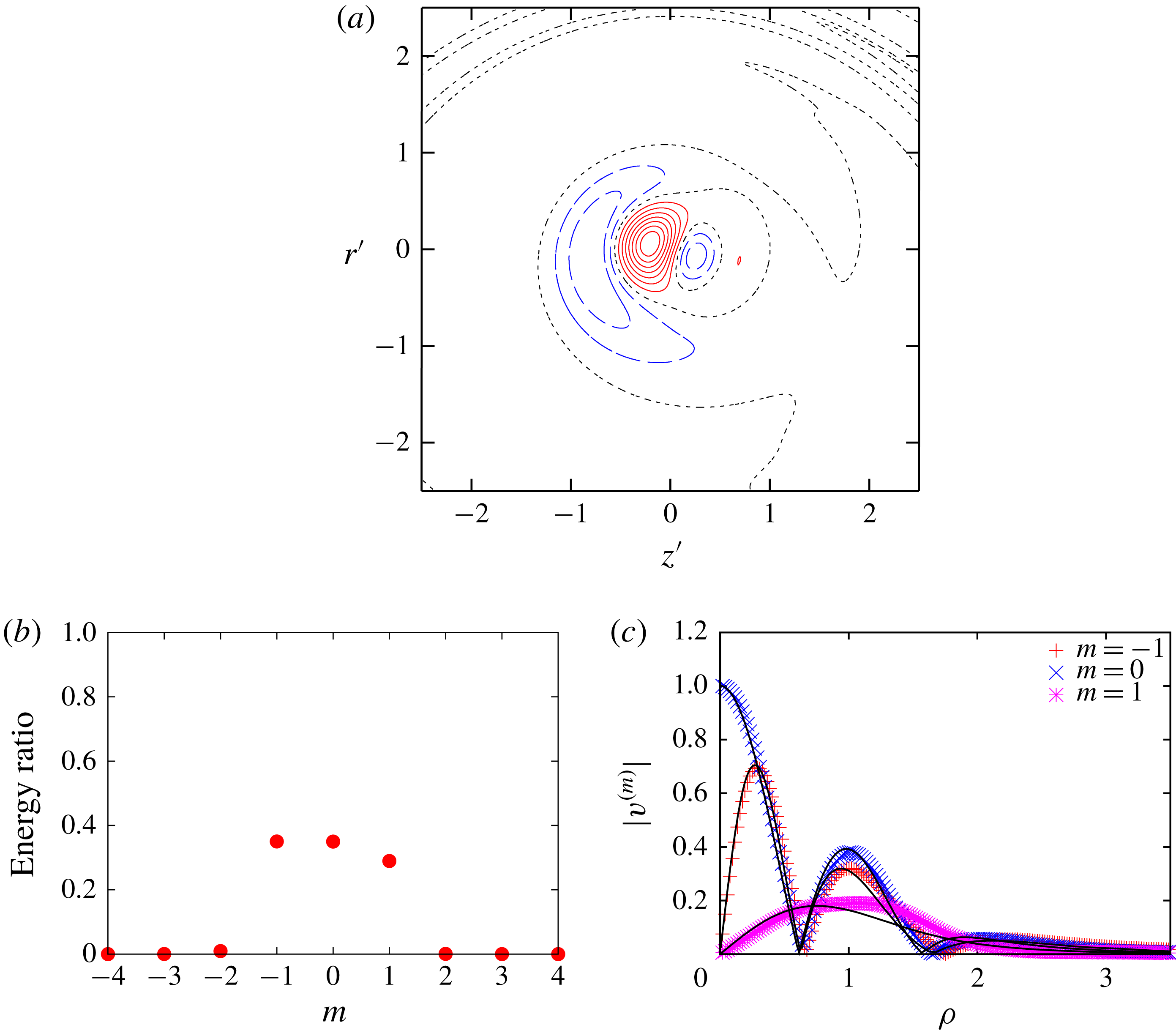
(dashed). (b) Ratio of energy. (c) Radial distribution of
 $v^{(m)}$
; symbols: DNS; lines: theory.

Figure 21 shows the three-wave mode of
 $(k,\unicode[STIX]{x1D714})=(1.389,-0.106)$
for
 $W=0.4$
. It consists of the
 $m=-1,0$
and
 $1$
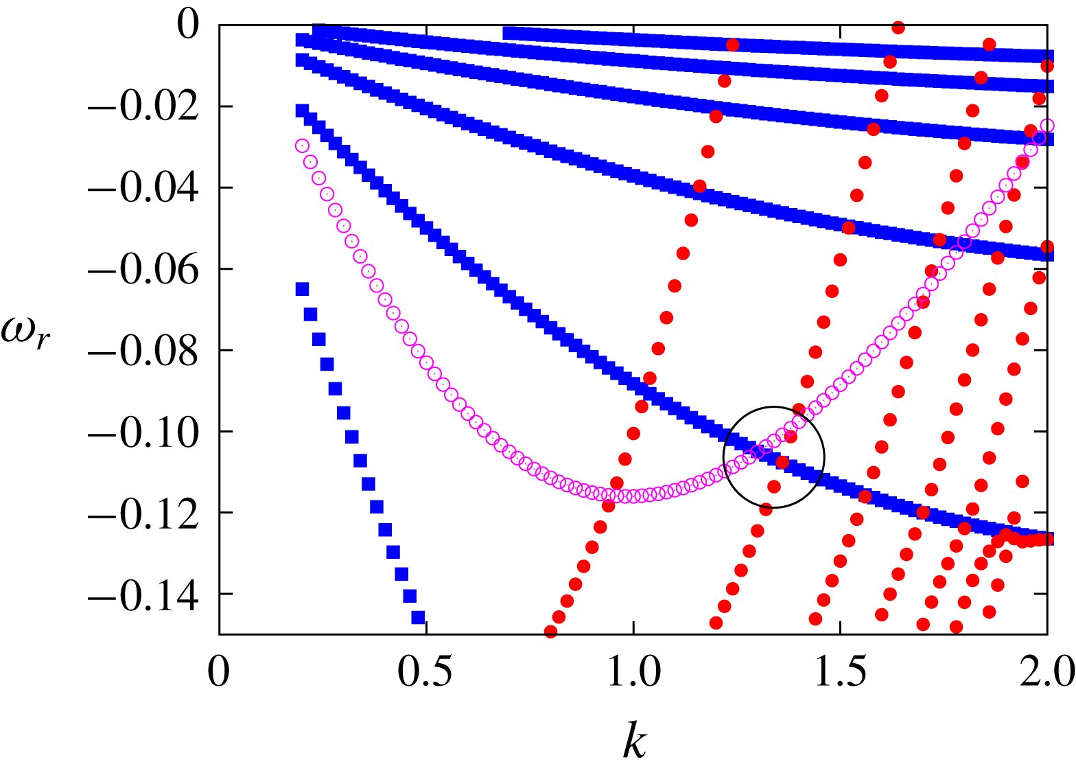
inertial waves. The energy ratios of the three waves are similar. The displacement mode (Fabre et al.
Reference Fabre, Sipp and Jacquin2006) of the
 $m=1$
wave happens to come close to the crossing point of the
 $m=-1$
and
 $m=0$
waves as shown in figure 22 so that the three waves interact with each other; thus, it is essentially a curvature instability mode. The interaction with the displacement mode would affect the growth rate; although it is of some interest to evaluate it analytically, it is avoided in the present paper since it requires elaborate calculations.
Dispersion curves. Here
 $Re=10^{4},W=0.4$
. Filled circles:
 $m=-1$
; squares:
 $m=0$
; open circles:
 $m=1$
(displacement mode). The large circle marks the crossing point of the three-wave mode.

4.3.3 Spiral mode
Spiral mode
 $(-1,0),k=4.231,\unicode[STIX]{x1D714}=-0.078$
. Here
 $W=0.4$
,
 $Re=10^{4},\unicode[STIX]{x1D700}_{0}=0.1$
. (a) Contours of azimuthal component of vorticity
 $\unicode[STIX]{x1D714}_{\unicode[STIX]{x1D703}}$
:
 $\unicode[STIX]{x1D714}_{\unicode[STIX]{x1D703}}>0$
(solid),
 $\unicode[STIX]{x1D714}_{\unicode[STIX]{x1D703}}=0$
(dotted) and
 $\unicode[STIX]{x1D714}_{\unicode[STIX]{x1D703}}<0$
(dashed). (b) Ratio of energy. (c) Radial distribution of
 $v^{(m)}$
; symbols: DNS; lines: theory.

Spiral mode
 $(-1,0),k=4.231,\unicode[STIX]{x1D714}=-0.078$
. Here
 $W=0.4$
,
 $Re=10^{4},\unicode[STIX]{x1D700}_{0}=0.18$
. (a) Contours of azimuthal component of vorticity
 $\unicode[STIX]{x1D714}_{\unicode[STIX]{x1D703}}$
:
 $\unicode[STIX]{x1D714}_{\unicode[STIX]{x1D703}}>0$
(solid),
 $\unicode[STIX]{x1D714}_{\unicode[STIX]{x1D703}}=0$
(dotted) and
 $\unicode[STIX]{x1D714}_{\unicode[STIX]{x1D703}}<0$
(dashed). (b) Ratio of energy. (c) Radial distribution of
 $v^{(m)}$
; symbols: DNS; lines: theory.

Figure 23 shows the spiral mode with
 $k=4.231$
for
 $W=0.4$
. It consists of
 $m=-1$
and
 $m=0$
waves; the energy ratio of the
 $m=0$
wave is much larger than that of the
 $m=-1$
wave. This
 $m=-1$
wave cannot be identified in the dispersion curves. Ring structures of strong azimuthal vorticity are observed for
 $1.4a\lesssim \unicode[STIX]{x1D70C}\lesssim 2a$
; correspondingly in this region of
 $\unicode[STIX]{x1D70C}$
the radial distribution of the
 $m=0$
wave differs between theoretical and numerical results. This spiral mode is similar to those observed in Roy et al. (Reference Roy, Schaeffer, Le Dizès and Thompson2008). It seems that this kind of modes appears at large wavenumbers and high Reynolds numbers.
In order to explore the nature of this instability mode, the case with thinner (
 $\unicode[STIX]{x1D700}_{0}=0.05$
) and thicker (
 $\unicode[STIX]{x1D700}_{0}=0.18$
) core is investigated. For
 $\unicode[STIX]{x1D700}_{0}=0.05$
, no instability is found. For
 $\unicode[STIX]{x1D700}_{0}=0.18$
, an unstable mode having spiral structures similar to those of
 $\unicode[STIX]{x1D700}_{0}=0.1$
(figure 23
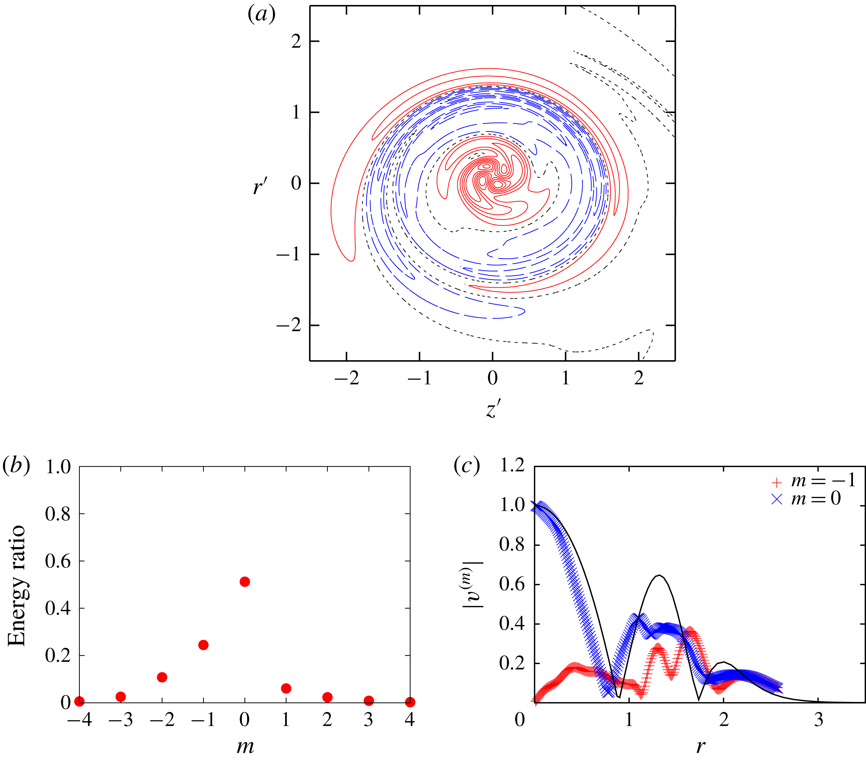
a) is found (figure 24). However, the energy ratio is much different; the
 $m=-1$
and
 $m=0$
waves have
 $24.5\,\%$
and
 $51.2\,\%$
of the total energy, respectively, while they are
 $13.1\,\%$
and
 $77.6\,\%$
for
 $\unicode[STIX]{x1D700}_{0}=0.1$
(figure 23
b). Since the amplitude of the mode is proportional to the square root of the energy, the amplitude ratio of the
 $m=-1$
wave to the
 $m=0$
wave for
 $\unicode[STIX]{x1D700}_{0}=0.18$
is
 $\sqrt{0.245/0.512}=0.692$
and that for
 $\unicode[STIX]{x1D700}_{0}=0.1$
is
 $\sqrt{0.131/0.776}=0.411$
; thus the amplitude ratio for
 $\unicode[STIX]{x1D700}_{0}=0.18$
is
 $0.692/0.411=1.68$
times larger than that for
 $\unicode[STIX]{x1D700}_{0}=0.1$
. This ratio is close to that of
 $\unicode[STIX]{x1D700}_{0}$
:
 $1.68\approx 0.18/0.1=1.8$
. This suggests that this
 $m=-1$
wave is not an inertial wave since the amplitude ratio should be independent of
 $\unicode[STIX]{x1D700}_{0}$
at the leading order for parametric resonance. Instead it can be
 $O(\unicode[STIX]{x1D700})$
component created by the
 $m=0$
wave and the
 $O(\unicode[STIX]{x1D700})$
dipole component of the base flow. The growth rate for
 $\unicode[STIX]{x1D700}_{0}=0.18$
is
 $\unicode[STIX]{x1D70E}=0.0193$
, which is
 $3.8$
times larger than that for
 $\unicode[STIX]{x1D700}_{0}=0.1$
. This suggests that the growth rate of the spiral mode is essentially proportional to
 $\unicode[STIX]{x1D700}_{0}^{2}$
as the value
 $3.8$
is not far from
 $(0.18/0.1)^{2}=3.24$
. It may be explained as the resonance of the
 $m=0$
wave of
 $O(1)$
and the
 $m=-1$
wave of
 $O(\unicode[STIX]{x1D700})$
by the
 $O(\unicode[STIX]{x1D700})$
dipole field, although further studies are required to understand these spiral modes.
5 Nonlinear effects
Although the main focus of the present paper is the linear instability of a vortex ring, it is also of interest and importance to investigate nonlinear time evolution of a disturbed vortex ring. We investigate nonlinear evolution of a vortex ring disturbed by a curvature instability mode focusing on the weakly nonlinear saturation.
The full nonlinear Navier–Stokes equations are solved; the Fourier spectral method is also used in the
 $\unicode[STIX]{x1D703}$
direction. The curvature instability mode of
 $(-1,0;[2,4])$
with
 $\unicode[STIX]{x1D700}_{0}=0.18$
for
 $W=0.2$
is chosen as the initial disturbance. Grid A in table 2 is used in the
 $r$
and
 $z$
directions. We assume
 $N_{\unicode[STIX]{x1D703}}$
-fold symmetry in
 $\unicode[STIX]{x1D703}$
, where
 $N_{\unicode[STIX]{x1D703}}$
is set to
 $10$
. This implies that subharmonic waves of the initial disturbance are excluded. The number of modes in the
 $\unicode[STIX]{x1D703}$
direction is
 $128$
. The Reynolds number is set to
 $Re=5000$
and
 $10^{4}$
, where the former value is used to accommodate the smallest structures that develop at the nonlinear stage. The initial energy of the disturbance is
 $0.0076\,\%$
and
 $0.0093\,\%$
of the base flow energy for
 $Re=5000$
and
 $10^{4}$
, respectively, while the effects of the initial energy are investigated for the latter case. It is pointed out that as time proceeds the core size of the vortex ring increases and the azimuthal velocity decreases because of viscous diffusion. This implies that the resonance condition of the curvature instability initially satisfied may be broken later.
Time evolution of the disturbance energy obtained by nonlinear simulation. The disturbance energy is decomposed in
 $\unicode[STIX]{x1D703}$
:
 $E_{n}=\int |\tilde{\boldsymbol{u}}_{n}|^{2}r\,\text{d}r\,\text{d}z$
, where the velocity field is decomposed as
 $\boldsymbol{u}=\sum _{n}\tilde{\boldsymbol{u}}_{n}(t,r,z)\text{e}^{\text{i}nN_{\unicode[STIX]{x1D703}}\unicode[STIX]{x1D703}}$
.

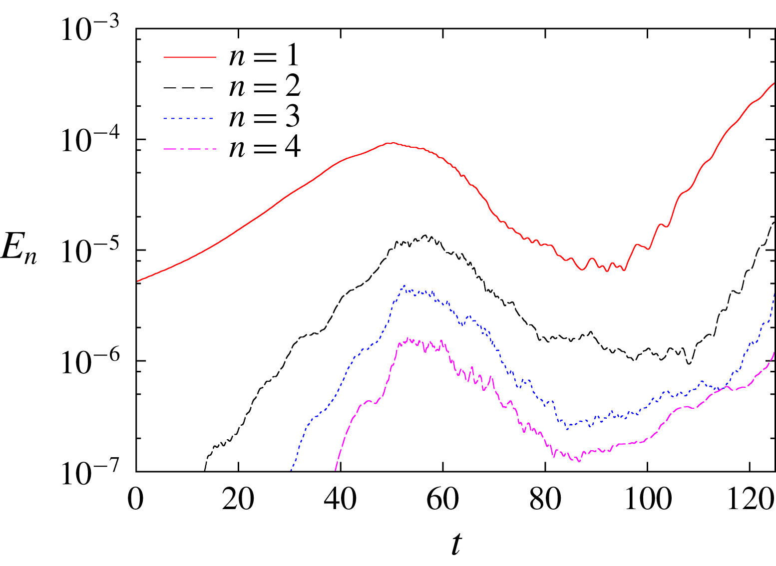
Figure 25 shows the time evolution of the disturbance energy decomposed in
 $\unicode[STIX]{x1D703}$
:
 $E_{n}=\int |\tilde{\boldsymbol{u}}_{n}|^{2}r\,\text{d}r\,\text{d}z$
, where the velocity field is decomposed as
 $\boldsymbol{u}=\sum _{n}\tilde{\boldsymbol{u}}_{n}(t,r,z)\text{e}^{\text{i}nN_{\unicode[STIX]{x1D703}}\unicode[STIX]{x1D703}}$
. At first the curvature instability mode (
 $n=1$
) grows exponentially. The growth rate is
 $\unicode[STIX]{x1D70E}=0.00803$
at
 $t=25$
; it is smaller than the observed value of
 $0.0113$
for
 $Re=10^{4}$
(figure 11) since viscous damping is stronger for
 $Re=5000$
. The higher-order modes
 $n\geqslant 2$
appear and grow faster than the main disturbance
 $n=1$
. The growth stops at
 $t\approx 50$
. Then the mode energy decreases exponentially, while the
 $n=1$
mode approaches the initial value at
 $t\approx 90$
. This is a typical behaviour predicted by weakly nonlinear analysis as explained later in some detail. Thus the peak at
 $t\approx 50$
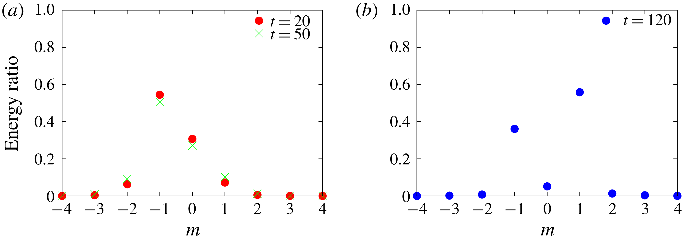
is due to weakly nonlinear saturation. Figure 26(a) shows the energy ratio of the
 $n=1$
mode at
 $t=20$
and
 $50$
. This confirms that the instability is due to the curvature instability as the energy ratio is close to that of the
 $(-1,0;[2,4])$
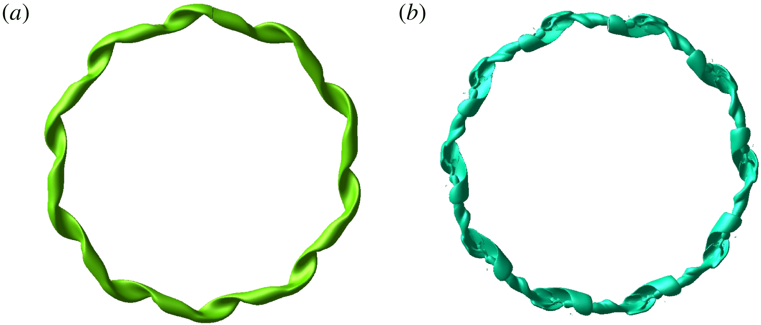
mode shown in figure 12(b). The structures of the whole vortex ring are shown in figure 27. Distortion of the ring is nearly due to the curvature instability mode at
 $t=25$
, while small-scale structures are visible at
 $t=50$
.
The mode energy starts growing again at
 $t\approx 95$
. The exponential growth rate is larger than that of the initial growth. This is due to the elliptic instability as shown below. Figure 26(b) shows the energy ratio of the
 $n=1$
mode at
 $t=120$
. It consists of
 $m=\pm 1$
waves. This elliptic instability mode corresponds to
 $(-1,1;[1,1])$
, which is shown in figure 8 for
 $W=0$
. Although the core size and the swirl parameter are set to
 $\unicode[STIX]{x1D700}=0.18$
and
 $W=0.2$
, respectively, at
 $t=0$
, they become
 $\unicode[STIX]{x1D700}\approx 0.3$
and
 $W\approx 0.12$
, respectively, at
 $t=120$
(figure 31); as a result the resonance condition for parametric instability moves from the curvature instability mode
 $(-1,0;[2,4])$
to the elliptic instability mode
 $(-1,1;[1,1])$
.
Ratio of energy of the linear mode
 $\tilde{\boldsymbol{u}}_{1}(t,r,z)$
obtained by nonlinear simulation. The linear mode is decomposed in the local polar coordinate system as in (4.1). (a) Time
 $t=20,50$
; (b)
 $t=120$
.

Structure of disturbed vortex ring obtained by nonlinear simulation. The isosurface of the magnitude of vorticity is shown. (a) Time
 $t=25$
; (b)
 $t=50$
.

Effects of the initial amplitude of the disturbance are investigated for
 $Re=10^{4}$
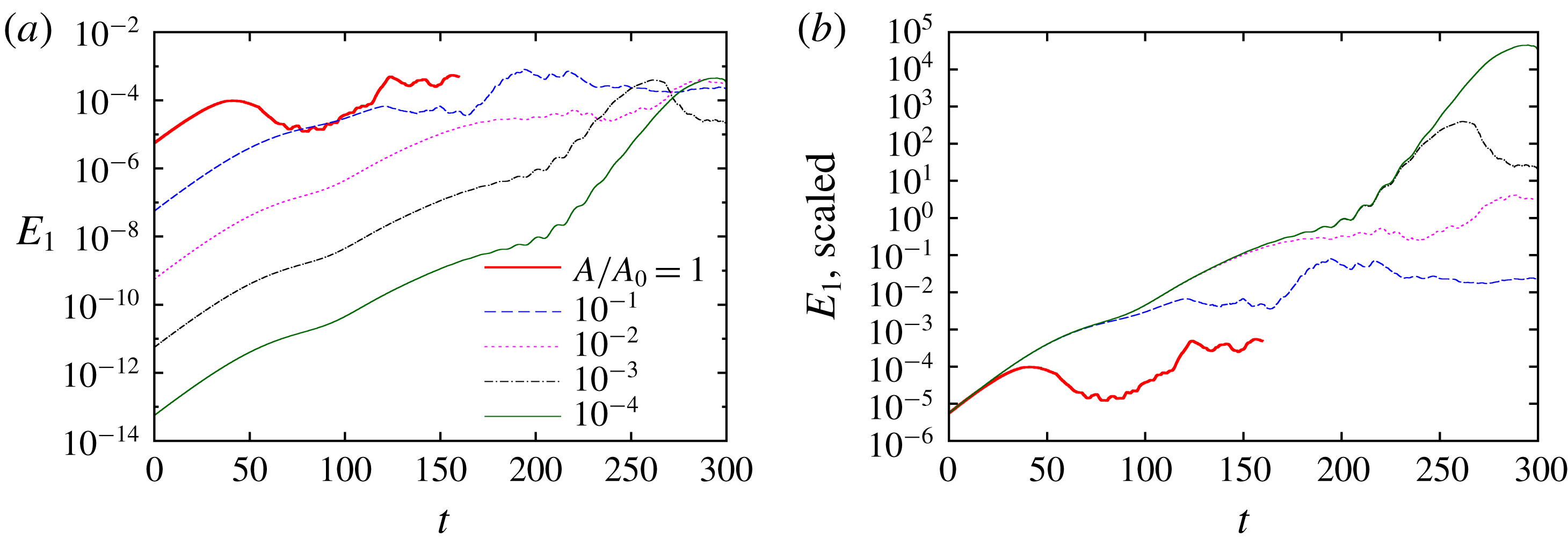
to clarify how nonlinearity leads to saturation of the curvature instability. Figure 28 compares time evolution of the energy of the linear mode
 $E_{1}$
for different values of the initial amplitude
 $A/A_{0}=1,10^{-1},\ldots ,10^{-4}$
. Figure 28(a) shows that
 $E_{1}$
saturates at
 $t=40.9,121.2$
and
 $189.1$
for
 $A/A_{0}=1,10^{-1}$
and
 $10^{-2}$
, respectively. The fact that
 $E_{1}\approx 10^{-4}$
does not depend on the initial amplitude very much supports that the saturation is due to weakly nonlinear effects. On the other hand, the elliptic instability takes over the curvature instability at
 $t\approx 200$
for
 $A/A_{0}=10^{-3}$
and
 $10^{-4}$
before saturation. In figure 28(b) the time evolutions of
 $E_{1}$
are divided by
 $(A/A_{0})^{2}$
so that they collapse at
 $t\approx 0$
. The time evolution starts to deviate from those for lower initial amplitudes when nonlinear effects become important. This shows that nonlinearity starts to affect the dynamics at
 $t\approx 20,90$
and
 $170$
for
 $A/A_{0}=1,10^{-1}$
and
 $10^{-2}$
, which are
 $20$
–
 $30$
before the saturation.
Time evolution of the disturbance energy obtained by nonlinear simulation. Here
 $Re=10^{4}$
. (a) The disturbance energy of the linear mode
 $E_{1}$
is compared for different values of the initial disturbance energy. (b) Same as (a) but the values are scaled to collapse at
 $t=0$
.

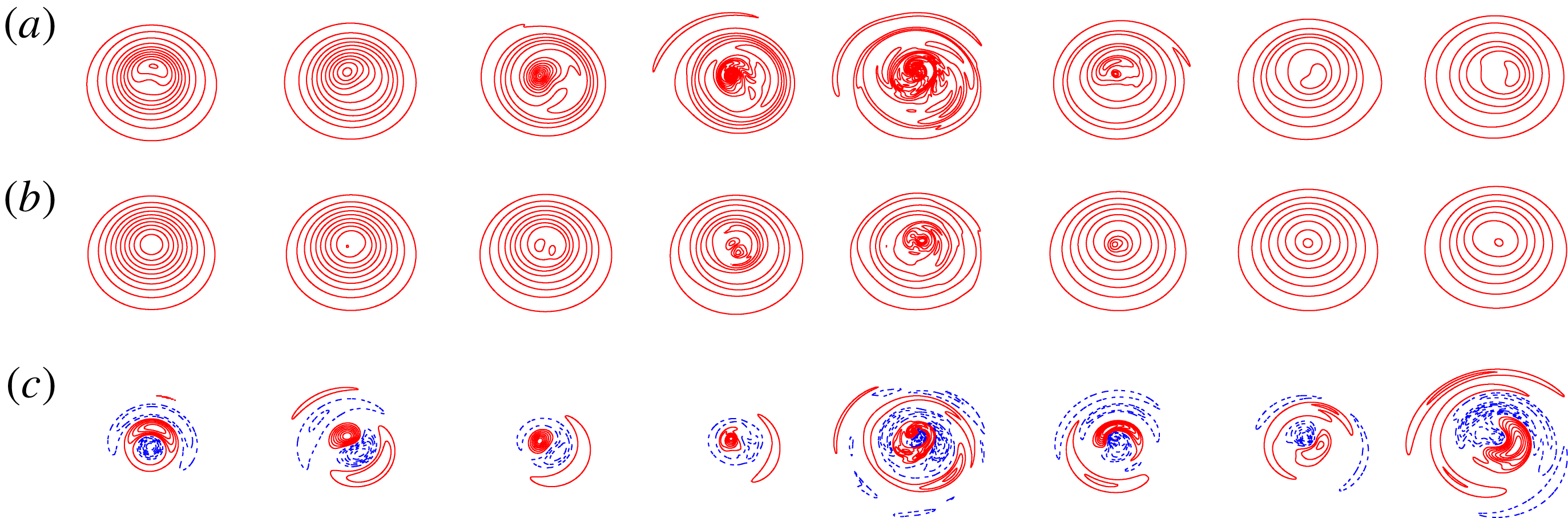
Figure 29 shows time evolution of the vortex ring by distribution of the
 $\unicode[STIX]{x1D703}$
component of vorticity on a cross-section (
 $\unicode[STIX]{x1D703}=0$
). The total vorticity
 $\unicode[STIX]{x1D714}_{\unicode[STIX]{x1D703}}$
(a), the mean vorticity
 $\tilde{\unicode[STIX]{x1D714}}_{\unicode[STIX]{x1D703},0}$
(b) and the disturbance vorticity
 $\unicode[STIX]{x1D714}_{\unicode[STIX]{x1D703}}-\tilde{\unicode[STIX]{x1D714}}_{\unicode[STIX]{x1D703},0}$
(c) are shown for
 $t=0,16,32,48,64,80,96$
and
 $112$
. It is pointed out that the contour levels are fixed for the total and mean vorticity, while they depend on the maximum value for the disturbance vorticity since the magnitude varies significantly with time. The total vorticity is significantly disturbed at
 $t=32,48$
and
 $64$
when the disturbance energy is large, while it goes back to smooth state at
 $t=96$
and
 $112$
. The same trend is also observed for the mean vorticity with lower level of disturbance. The distribution of the disturbance vorticity does not differ much from the curvature instability mode of
 $(-1,0;[2,4])$
up to
 $t=48$
. However, the distribution changes after
 $t=48$
; at
 $t=96$
and
 $112$
it shows structures of bending wave due to the elliptic instability.
Time evolution of disturbed vortex ring. Contours of
 $\unicode[STIX]{x1D703}$
component of vorticity on
 $\unicode[STIX]{x1D703}=0$
are shown. Here
 $Re=5000$
. Total vorticity
 $\unicode[STIX]{x1D714}_{\unicode[STIX]{x1D703}}$
(a), mean vorticity
 $\tilde{\unicode[STIX]{x1D714}}_{\unicode[STIX]{x1D703},0}$
(b), disturbance vorticity
 $\unicode[STIX]{x1D714}_{\unicode[STIX]{x1D703}}-\tilde{\unicode[STIX]{x1D714}}_{\unicode[STIX]{x1D703},0}$
(c). From left to right:
 $t=0,16,32,48,64,80,96,112$
. Contour levels are
 $n\unicode[STIX]{x0394}\unicode[STIX]{x1D714}$
(
 $n=\pm 1,\pm 2,\ldots$
) while
 $\unicode[STIX]{x0394}\unicode[STIX]{x1D714}=1$
for the total and mean vorticity and
 $\unicode[STIX]{x0394}\unicode[STIX]{x1D714}=|\unicode[STIX]{x1D714}_{\unicode[STIX]{x1D703}}-\tilde{\unicode[STIX]{x1D714}}_{\unicode[STIX]{x1D703},0}|_{max}/8$
for the disturbance vorticity. Positive and negative values are shown by red and blue lines, respectively.

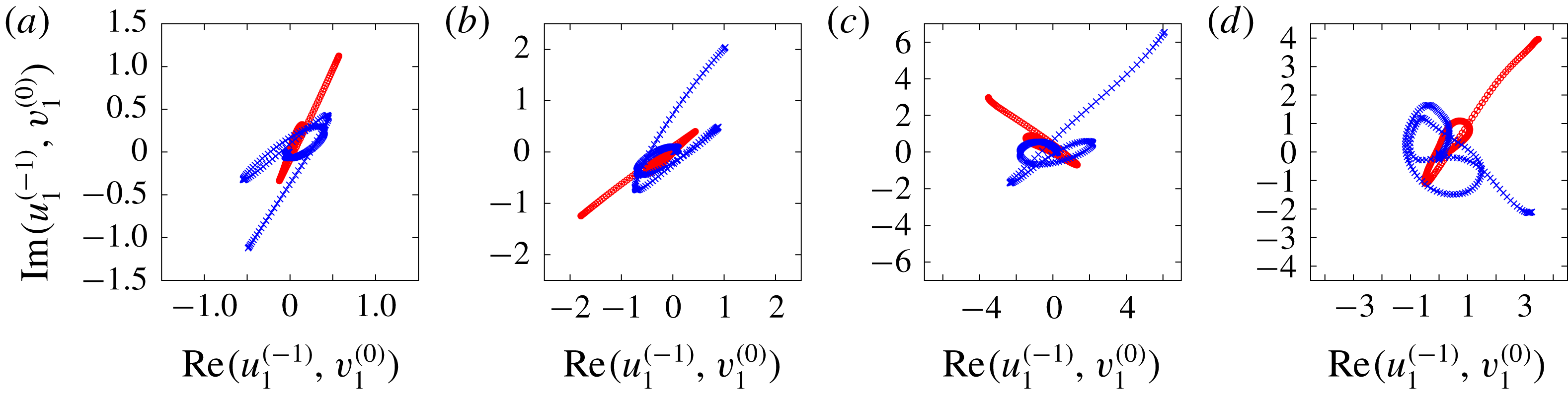
Linear modes on the complex plane. The linear modes are decomposed in the local coordinate system
 $(\unicode[STIX]{x1D70C},\unicode[STIX]{x1D719})$
, and
 $\tilde{u} _{1}^{(-1)}$
(shown by red circles) and
 $\tilde{v}_{1}^{(0)}$
(shown by blue crosses) are plotted on the complex plane. Here
 $Re=5000$
. (a) Time
 $t=0$
, (b)
 $t=20$
, (c)
 $t=48$
, (d)
 $t=60$
.

The details of weakly nonlinear saturation can be shown by the phases of the
 $m=-1$
and
 $m=0$
waves which compose the curvature instability mode. Figure 30 shows those waves on the complex plane for
 $t=0,20,48$
and
 $60$
. The linear mode
 $\tilde{\boldsymbol{u}}_{1}(t,r,z)$
is decomposed in the local coordinate system (figure 1) and
 $\tilde{u} _{1}^{(-1)}$
and
 $\tilde{v}_{1}^{(0)}$
are shown by red circles and blue crosses, respectively. The curves rotate with time since the two waves are oscillatory. The curves at
 $t=0$
and
 $t=20$
are similar in shape after rotation, while they deform gradually as time proceeds (
 $t=48$
and
 $60$
). The phase difference between
 $\tilde{u} _{1}^{(-1)}$
and
 $\tilde{v}_{1}^{(0)}$
is important here. We take the phase at maximum amplitude for each mode. Then the phase difference is
 $-177^{\circ },-151^{\circ },-93^{\circ }$
and
 $-82^{\circ }$
at
 $t=0,20,48$
and
 $60$
, respectively. The value of phase difference depends on the section or
 $\unicode[STIX]{x1D703}$
. An important point is that the phase difference increases with
 $84^{\circ }\approx \unicode[STIX]{x03C0}/2$
from the initial state
 $t=0$
to
 $t=48$
at which the curvature instability saturates. This change in the phase difference is explained in terms of the amplitude equation derived by weakly nonlinear analysis. In the simplest form, the amplitude equation is
 $$\begin{eqnarray}\displaystyle \frac{\text{d}A_{-1}}{\text{d}t} & = & \displaystyle c_{1}A_{0}+\text{i}(s_{1}|A_{-1}|^{2}+s_{2}|A_{0}|^{2})A_{-1},\end{eqnarray}$$
 $$\begin{eqnarray}\displaystyle \frac{\text{d}A_{0}}{\text{d}t} & = & \displaystyle c_{2}A_{-1}+\text{i}(s_{3}|A_{-1}|^{2}+s_{4}|A_{0}|^{2})A_{0},\end{eqnarray}$$
where
 $A_{-1}$
and
 $A_{0}$
are the complex amplitudes of the
 $m=-1$
and
 $m=0$
waves and
 $c_{i}$
and
 $s_{i}$
are real constants satisfying
 $c_{1}c_{2}>0$
(Knobloch, Mahalov & Marsden Reference Knobloch, Mahalov and Marsden1994). At the linear stage
 $|A_{-1}|$
and
 $|A_{0}|$
are sufficiently small so that the nonlinear terms are negligible; then the phase difference between
 $A_{-1}$
and
 $A_{0}$
is
 $0$
for the exponentially growing solution to equations (5.1) and (5.2). On the other hand, when the growth saturates, which implies
 $\text{d}A_{-1}/\text{d}t=\text{d}A_{0}/\text{d}t=0$
, the phase difference between
 $A_{-1}$
and
 $A_{0}$
is
 $\unicode[STIX]{x03C0}/2$
according to (5.1) and (5.2); in other words, the detuning effects of nonlinear terms stop the curvature instability. Thus the phase difference increases with
 $\unicode[STIX]{x03C0}/2$
when the growth saturates. Therefore, the change in the phase difference observed in figure 30 is a result of weakly nonlinear saturation described by the amplitude equation (Sipp Reference Sipp2000; Eloy, Le Gal & Le Dizès Reference Eloy, Le Gal and Le Dizès2000, Reference Eloy, Le Gal and Le Dizès2003).
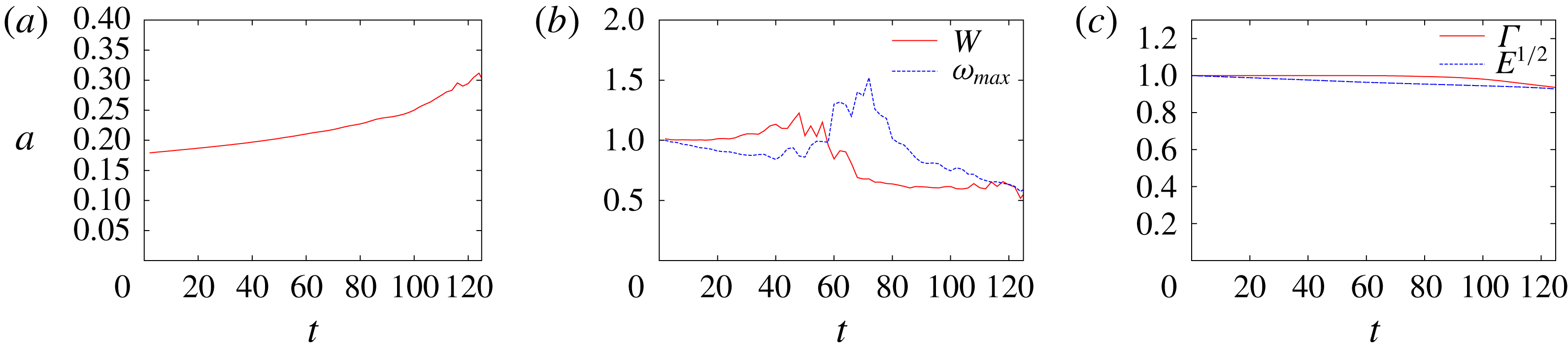
Figure 31 shows time evolution of characteristic values of the vortex ring: the core radius, the swirl parameter
 $W$
, the maximum vorticity, the circulation and the energy. Here the values are normalized by the initial values except for the core radius and the energy is plotted with its square root to be proportional to the velocity for comparison. The figure shows that the swirl parameter increases gradually before nonlinear saturation, then it drops at
 $48\lesssim t\lesssim 64$
. Correspondingly, the maximum vorticity decreases before nonlinear saturation, then it increases at
 $48\lesssim t\lesssim 70$
. Thus there are changes in the mean flow after nonlinear saturation. The viscous spreading of the core is slightly accelerated after the saturation (figure 31
a), although the circulation is nearly constant up to
 $t\approx 80$
and the decay of the energy is unaffected up to
 $t\approx 120$
(figure 31
c).
Time evolution of characteristic values of the vortex ring. Here
 $Re=5000$
. (a) Core radius, (b) swirl parameter and maximum vorticity, (c) circulation and square root of energy. Note that the values are normalized by the initial values for comparison.

To summarize, the curvature instability grows until weakly nonlinear saturation; after the saturation nonlinear effects modify the mean flow decreasing the swirl parameter and the disturbance energy decreases. It is pointed out that the secondary instability following the curvature instability is not observed.
6 Concluding remarks
We have studied the linear instability of a vortex ring with swirl with Gaussian distributions of azimuthal vorticity and velocity in its core at the leading order of the thickness by DNS: the quasi-steady base flow was obtained by solving the axisymmetric incompressible Navier–Stokes equations, then the linearized Navier–Stokes equations were solved by DNS. It was shown that the vortex rings are subjected to curvature instability as predicted analytically by Blanco-Rodríguez & Le Dizès (Reference Blanco-Rodríguez and Le Dizès2017). The structures of the unstable modes obtained numerically are in good agreement with the analytical results. For the growth rates, on the other hand, some differences between numerical and analytical results were found depending on the unstable mode. The differences are most likely due to the critical layer damping which is evaluated for the waves on axisymmetric line vortices in the analysis; the actual growth rate is affected by the deformation of the core since the damping is sensitive to the position of the critical layer. Competition between the curvature and elliptic instabilities was also investigated. When the swirl is absent, only the elliptic instability is observed since the growth rate of the curvature instability is small. When the swirl is added, sharp bands of the two instabilities are observed for small thickness
 $\unicode[STIX]{x1D700}\approx 0.1$
, while the elliptic instability dominates except for a small interval of the wavenumber for
 $\unicode[STIX]{x1D700}\approx 0.18$
. A special mode which consists of three waves was also found; although it is essentially due to the curvature instability mode of
 $(-1,0;[2,2])$
, a displacement wave of
 $m=1$
happens to be close to the corresponding crossing point of the dispersion curves and joins the unstable mode. Spiral modes which may be due to
 $O(\unicode[STIX]{x1D700}^{2})$
effects were also found. Weakly nonlinear saturation has been shown to occur by nonlinear simulation.
It is emphasized that the curvature instability has been shown by DNS for the first time; although by theoretical analysis it was first shown for Kelvin’s vortex ring (Hattori & Fukumoto Reference Hattori and Fukumoto2003; Fukumoto & Hattori Reference Fukumoto and Hattori2005) and then for a Gaussian vortex ring (Blanco-Rodríguez & Le Dizès Reference Blanco-Rodríguez and Le Dizès2017), no results from numerical simulation or experiments have been available before the present work. The present results should be taken into account carefully in interpreting the experimental results since the curvature instability can be the dominant instability for large Reynolds numbers and small thickness. In the numerical work by Gargan-Shingles et al. (Reference Gargan-Shingles, Rudman and Ryan2016), the Reynolds number is smaller than in the the present work:
 $Re=10^{4}/(2\unicode[STIX]{x03C0})=1592$
. In addition, the thickness is larger:
 $a/R=0.234$
–
 $0.344$
. These are the reasons why they did not observe the curvature instability, although the mode shown in figure 9A of Gargan-Shingles et al. (Reference Gargan-Shingles, Rudman and Ryan2016) may be due to curvature instability. Another result worth emphasizing is that the critical layer damping is sensitive to the deformation of the vortex core; the growth rate of the curvature instability mode
 $(-1,0;[1,3])$
at
 $\unicode[STIX]{x1D700}_{0}=0.1$
was found to be
 $22\,\%$
smaller than the theoretical value, while it is in good agreement for the mode
 $(-1,0;[2,4])$
. This difference is most likely due to the critical layer damping which is strong for the former but weak for the latter. This result is important not only for the curvature instability but also for any short-wave instability due to parametric resonance like elliptic instability and precession instability which occurs in a precessing cylinder (Kerswell Reference Kerswell1993; Mahalov Reference Mahalov1993; Lagrange et al.
Reference Lagrange, Eloy, Nadal and Meunier2008).
Finally, two important future works are mentioned briefly. First, nonlinear evolution of curvature instability modes should be investigated further to clarify their role in the dynamics of a vortex ring: it can lead to the breakdown of a vortex ring. Next, the curvature instability of a helical vortex should be explored; as shown theoretically by Hattori & Fukumoto (Reference Hattori and Fukumoto2009, Reference Hattori and Fukumoto2010, Reference Hattori and Fukumoto2012, Reference Hattori and Fukumoto2014) and Blanco-Rodríguez & Le Dizès (Reference Blanco-Rodríguez and Le Dizès2017), helical vortices are subjected to the curvature instability in general. This is of great importance since the helical vortices are a model of tip vortices generated by rotating wings like helicopter rotors, wind rotors and ship propellers. The curvature instability is expected to be important as the conditions for the curvature instability to be dominant are often satisfied for these rotating wings: the Reynolds number is large, the thickness is small and the base flow has a non-vanishing swirl. The numerical methods developed in Delbende, Rossi & Daube (Reference Delbende, Rossi and Daube2012) and Selçuk, Delbende & Rossi (Reference Selçuk, Delbende and Rossi2018) would be useful for this problem.
Acknowledgements
This work was supported by Collaborative Research Project 2016–2018, Institute of Fluid Science, Tohoku University. This work also received support from the French Agence Nationale de la Recherche under A*MIDEX grant ANR-11-IDEX-0001-02, the LABEX MEC project ANR-11-LABX-0092 and the ANR HELIX project ANR-12-BS09-0023-01. Y.H. is grateful to IRPHE for the kind hospitality during his visit. Numerical calculations were performed on the UV2000 at the Institute of Fluid Science, Tohoku University.
Appendix A. Details of numerical methods
In this appendix we describe the details of our numerical method. The incompressible Navier–Stokes equations are written as
 $$\begin{eqnarray}\displaystyle & \displaystyle \frac{\unicode[STIX]{x2202}u}{\unicode[STIX]{x2202}t}=-u\frac{\unicode[STIX]{x2202}u}{\unicode[STIX]{x2202}r}-\frac{v}{r}\frac{\unicode[STIX]{x2202}u}{\unicode[STIX]{x2202}\unicode[STIX]{x1D703}}-w\frac{\unicode[STIX]{x2202}u}{\unicode[STIX]{x2202}z}+\frac{v^{2}}{r}-\frac{\unicode[STIX]{x2202}p}{\unicode[STIX]{x2202}r}+\unicode[STIX]{x1D708}\left[\left(\unicode[STIX]{x1D6FB}^{2}-\frac{1}{r^{2}}\right)u-\frac{2}{r^{2}}\frac{\unicode[STIX]{x2202}v}{\unicode[STIX]{x2202}\unicode[STIX]{x1D703}}\right], & \displaystyle\end{eqnarray}$$
 $$\begin{eqnarray}\displaystyle & \displaystyle \frac{\unicode[STIX]{x2202}v}{\unicode[STIX]{x2202}t}=-u\frac{\unicode[STIX]{x2202}v}{\unicode[STIX]{x2202}r}-\frac{v}{r}\frac{\unicode[STIX]{x2202}v}{\unicode[STIX]{x2202}\unicode[STIX]{x1D703}}-w\frac{\unicode[STIX]{x2202}v}{\unicode[STIX]{x2202}z}-\frac{uv}{r}-\frac{1}{r}\frac{\unicode[STIX]{x2202}p}{\unicode[STIX]{x2202}\unicode[STIX]{x1D703}}+\unicode[STIX]{x1D708}\left[\left(\unicode[STIX]{x1D6FB}^{2}-\frac{1}{r^{2}}\right)v+\frac{2}{r^{2}}\frac{\unicode[STIX]{x2202}u}{\unicode[STIX]{x2202}\unicode[STIX]{x1D703}}\right], & \displaystyle\end{eqnarray}$$
 $$\begin{eqnarray}\displaystyle & \displaystyle \frac{\unicode[STIX]{x2202}w}{\unicode[STIX]{x2202}t}=-u\frac{\unicode[STIX]{x2202}w}{\unicode[STIX]{x2202}r}-\frac{v}{r}\frac{\unicode[STIX]{x2202}w}{\unicode[STIX]{x2202}\unicode[STIX]{x1D703}}-w\frac{\unicode[STIX]{x2202}w}{\unicode[STIX]{x2202}z}-\frac{\unicode[STIX]{x2202}p}{\unicode[STIX]{x2202}z}+\unicode[STIX]{x1D708}\unicode[STIX]{x1D6FB}^{2}w, & \displaystyle\end{eqnarray}$$
 $$\begin{eqnarray}\displaystyle & \displaystyle \frac{\unicode[STIX]{x2202}u}{\unicode[STIX]{x2202}r}+\frac{u}{r}+\frac{1}{r}\frac{\unicode[STIX]{x2202}v}{\unicode[STIX]{x2202}\unicode[STIX]{x1D703}}+\frac{\unicode[STIX]{x2202}w}{\unicode[STIX]{x2202}z}=0, & \displaystyle\end{eqnarray}$$
where
 $u,v$
and
 $w$
are the
 $r$
,
 $\unicode[STIX]{x1D703}$
and
 $z$
components of the velocity and
 $\unicode[STIX]{x1D6FB}^{2}=\unicode[STIX]{x2202}^{2}/\unicode[STIX]{x2202}r^{2}+(1/r)\unicode[STIX]{x2202}/\unicode[STIX]{x2202}r+(1/r^{2})\unicode[STIX]{x2202}^{2}/\unicode[STIX]{x2202}\unicode[STIX]{x1D703}^{2}+\unicode[STIX]{x2202}^{2}/\unicode[STIX]{x2202}z^{2}$
. The above equations are discretized in time with the second-order implicit method for the viscous terms and the Adams–Bashforth method for the other terms:
 $$\begin{eqnarray}\displaystyle \left[\frac{3}{2}-\unicode[STIX]{x1D708}\unicode[STIX]{x0394}t\unicode[STIX]{x1D6FB}^{2}\right]u^{(n+1)} & = & \displaystyle 2u^{(n)}-\frac{1}{2}u^{(n-1)}+\frac{\unicode[STIX]{x0394}t}{2}(3H_{u}^{(n)}-H_{u}^{(n-1)}),\end{eqnarray}$$
 $$\begin{eqnarray}\displaystyle \left[\frac{3}{2}-\unicode[STIX]{x1D708}\unicode[STIX]{x0394}t\unicode[STIX]{x1D6FB}^{2}\right]v^{(n+1)} & = & \displaystyle 2v^{(n)}-\frac{1}{2}v^{(n-1)}+\frac{\unicode[STIX]{x0394}t}{2}(3H_{v}^{(n)}-H_{v}^{(n-1)}),\end{eqnarray}$$
 $$\begin{eqnarray}\displaystyle \left[\frac{3}{2}-\unicode[STIX]{x1D708}\unicode[STIX]{x0394}t\unicode[STIX]{x1D6FB}^{2}\right]w^{(n+1)} & = & \displaystyle 2w^{(n)}-\frac{1}{2}w^{(n-1)}+\frac{\unicode[STIX]{x0394}t}{2}(3H_{w}^{(n)}-H_{w}^{(n-1)}),\end{eqnarray}$$
where
 $f^{(n)}$
denotes
 $f$
at the
 $n$
th time step,
 $$\begin{eqnarray}\displaystyle H_{u} & = & \displaystyle h_{u}-\frac{\unicode[STIX]{x2202}\unicode[STIX]{x1D6F7}}{\unicode[STIX]{x2202}r},\end{eqnarray}$$
 $$\begin{eqnarray}\displaystyle H_{v} & = & \displaystyle h_{v}-\frac{1}{r}\frac{\unicode[STIX]{x2202}\unicode[STIX]{x1D6F7}}{\unicode[STIX]{x2202}\unicode[STIX]{x1D703}},\end{eqnarray}$$
 $$\begin{eqnarray}\displaystyle H_{w} & = & \displaystyle h_{w}-\frac{\unicode[STIX]{x2202}\unicode[STIX]{x1D6F7}}{\unicode[STIX]{x2202}z},\end{eqnarray}$$
and
 $$\begin{eqnarray}\displaystyle h_{u} & = & \displaystyle -u\frac{\unicode[STIX]{x2202}u}{\unicode[STIX]{x2202}r}-\frac{v}{r}\frac{\unicode[STIX]{x2202}u}{\unicode[STIX]{x2202}\unicode[STIX]{x1D703}}-w\frac{\unicode[STIX]{x2202}u}{\unicode[STIX]{x2202}z}+\frac{v^{2}}{r}+\unicode[STIX]{x1D708}\left(-\frac{u}{r^{2}}-\frac{2}{r^{2}}\frac{\unicode[STIX]{x2202}v}{\unicode[STIX]{x2202}\unicode[STIX]{x1D703}}\right),\end{eqnarray}$$
 $$\begin{eqnarray}\displaystyle h_{v} & = & \displaystyle -u\frac{\unicode[STIX]{x2202}v}{\unicode[STIX]{x2202}r}-\frac{v}{r}\frac{\unicode[STIX]{x2202}v}{\unicode[STIX]{x2202}\unicode[STIX]{x1D703}}-w\frac{\unicode[STIX]{x2202}v}{\unicode[STIX]{x2202}z}-\frac{uv}{r}+\unicode[STIX]{x1D708}\left(-\frac{v}{r^{2}}+\frac{2}{r^{2}}\frac{\unicode[STIX]{x2202}u}{\unicode[STIX]{x2202}\unicode[STIX]{x1D703}}\right),\end{eqnarray}$$
 $$\begin{eqnarray}\displaystyle h_{w} & = & \displaystyle -u\frac{\unicode[STIX]{x2202}w}{\unicode[STIX]{x2202}r}-\frac{v}{r}\frac{\unicode[STIX]{x2202}w}{\unicode[STIX]{x2202}\unicode[STIX]{x1D703}}-w\frac{\unicode[STIX]{x2202}w}{\unicode[STIX]{x2202}z}.\end{eqnarray}$$
It should be pointed out that the cross terms in the viscous terms (e.g.
 $\unicode[STIX]{x1D708}(2/r^{2})\unicode[STIX]{x2202}v/\unicode[STIX]{x2202}\unicode[STIX]{x1D703}$
in (A 11)) are moved to the right-hand side together with the corresponding terms which cancel their divergent behaviour near
 $r=0$
(e.g.
 $\unicode[STIX]{x1D708}(u/r^{2})$
in (A 11)) as only the Laplacian terms are dealt with implicitly; this simplifies the numerical procedure. The function
 $\unicode[STIX]{x1D6F7}$
is obtained by solving the Poisson equation
 $$\begin{eqnarray}\displaystyle \unicode[STIX]{x1D6FB}^{2}\unicode[STIX]{x1D6F7}=\frac{\unicode[STIX]{x2202}h_{u}}{\unicode[STIX]{x2202}r}+\frac{h_{u}}{r}+\frac{1}{r}\frac{\unicode[STIX]{x2202}h_{v}}{\unicode[STIX]{x2202}\unicode[STIX]{x1D703}}+\frac{\unicode[STIX]{x2202}h_{w}}{\unicode[STIX]{x2202}z}. & & \displaystyle\end{eqnarray}$$
The boundary conditions at
 $r=\pm L_{r}$
are
 $$\begin{eqnarray}\displaystyle u=0,\quad \frac{\unicode[STIX]{x2202}}{\unicode[STIX]{x2202}r}(rv)=\frac{\unicode[STIX]{x2202}}{\unicode[STIX]{x2202}r}w=0. & & \displaystyle\end{eqnarray}$$
The velocity fields are expanded in Fourier series as
 $f=\sum _{n}\hat{f}_{m,n}(r,t)\text{e}^{\text{i}(m\unicode[STIX]{x1D703}+n\unicode[STIX]{x1D6FC}z)}$
, where
 $m=0$
for the base flow and
 $m=N_{\unicode[STIX]{x1D703}}$
for the disturbance and
 $\unicode[STIX]{x1D6FC}=2\unicode[STIX]{x03C0}/L_{z}$
. Then the equations in the Fourier space are
 $$\begin{eqnarray}\displaystyle & & \displaystyle \left[\frac{3}{2}-\unicode[STIX]{x1D708}\unicode[STIX]{x0394}t\left\{\frac{\text{d}^{2}}{\text{d}r^{2}}+\frac{1}{r}\frac{\text{d}}{\text{d}r}-\left(\frac{(|m|-1)^{2}}{r^{2}}+\unicode[STIX]{x1D6FC}^{2}n^{2}\right)\right\}\right]\hat{u} _{m,n}^{(n+1)}\nonumber\\ \displaystyle & & \displaystyle \quad =2\hat{u} _{m,n}^{(n)}-\frac{1}{2}\hat{u} _{m,n}^{(n-1)}+\frac{\unicode[STIX]{x0394}t}{2}(3{\hat{H}}_{u;m,n}^{(n)}-{\hat{H}}_{u;m,n}^{(n-1)}),\end{eqnarray}$$
 $$\begin{eqnarray}\displaystyle & & \displaystyle \left[\frac{3}{2}-\unicode[STIX]{x1D708}\unicode[STIX]{x0394}t\left\{\frac{\text{d}^{2}}{\text{d}r^{2}}+\frac{1}{r}\frac{\text{d}}{\text{d}r}-\left(\frac{(|m|-1)^{2}}{r^{2}}+\unicode[STIX]{x1D6FC}^{2}n^{2}\right)\right\}\right]\hat{v}_{m,n}^{(n+1)}\nonumber\\ \displaystyle & & \displaystyle \quad =2\hat{v}_{m,n}^{(n)}-\frac{1}{2}\hat{v}_{m,n}^{(n-1)}+\frac{\unicode[STIX]{x0394}t}{2}(3{\hat{H}}_{v;m,n}^{(n)}-{\hat{H}}_{v;m,n}^{(n-1)}),\end{eqnarray}$$
 $$\begin{eqnarray}\displaystyle & & \displaystyle \left[\frac{3}{2}-\unicode[STIX]{x1D708}\unicode[STIX]{x0394}t\left\{\frac{\text{d}^{2}}{\text{d}r^{2}}+\frac{1}{r}\frac{\text{d}}{\text{d}r}-\left(\frac{m^{2}}{r^{2}}+\unicode[STIX]{x1D6FC}^{2}n^{2}\right)\right\}\right]{\hat{w}}_{m,n}^{(n+1)}\nonumber\\ \displaystyle & & \displaystyle \quad =2{\hat{w}}_{m,n}^{(n)}-\frac{1}{2}{\hat{w}}_{m,n}^{(n-1)}+\frac{\unicode[STIX]{x0394}t}{2}(3{\hat{H}}_{w;m,n}^{(n)}-{\hat{H}}_{w;m,n}^{(n-1)}).\end{eqnarray}$$
The boundary conditions (A 15) become
 $$\begin{eqnarray}\displaystyle \hat{u} _{m,n}=0,\quad \frac{\unicode[STIX]{x2202}}{\unicode[STIX]{x2202}r}(r\hat{v}_{m,n})=\frac{\unicode[STIX]{x2202}{\hat{w}}_{m,n}}{\unicode[STIX]{x2202}r}=0. & & \displaystyle\end{eqnarray}$$
The Poisson equation for
 $\unicode[STIX]{x1D6F7}$
is also expressed in Fourier space as
 $$\begin{eqnarray}\displaystyle & & \displaystyle \left\{\frac{\text{d}^{2}}{\text{d}r^{2}}+\frac{1}{r}\frac{\text{d}}{\text{d}r}-\left(\frac{m^{2}}{r^{2}}+\unicode[STIX]{x1D6FC}^{2}n^{2}\right)\right\}\hat{\unicode[STIX]{x1D6F7}}_{m,n}\nonumber\\ \displaystyle & & \displaystyle \quad =\frac{\text{d}{\hat{h}}_{u;m,n}}{\text{d}r}+\frac{{\hat{h}}_{u;m,n}}{r}+\frac{\text{i}m}{r}{\hat{h}}_{v;m,n}+\text{i}\unicode[STIX]{x1D6FC}n{\hat{h}}_{w;m,n},\end{eqnarray}$$
with the boundary condition
 $$\begin{eqnarray}\displaystyle \frac{\unicode[STIX]{x2202}\hat{\unicode[STIX]{x1D6F7}}_{m,n}}{\unicode[STIX]{x2202}r}=0. & & \displaystyle\end{eqnarray}$$
Equations (A 16)–(A 18) and (A 20) for each Fourier mode are second-order ordinary differential equations; they are solved by a sixth-order accurate compact scheme.
The numerical method for the linear stability analysis is the same except that the nonlinear terms in
 $h_{u},h_{v}$
and
 $h_{w}$
are replaced by the corresponding linearized terms. For example,
 $h_{u}$
is replaced by
 $$\begin{eqnarray}\displaystyle {h^{\prime }}_{u} & = & \displaystyle -u_{b}\frac{\unicode[STIX]{x2202}u^{\prime }}{\unicode[STIX]{x2202}r}-\frac{v_{b}}{r}\frac{\unicode[STIX]{x2202}u^{\prime }}{\unicode[STIX]{x2202}\unicode[STIX]{x1D703}}-w_{b}\frac{\unicode[STIX]{x2202}u^{\prime }}{\unicode[STIX]{x2202}z}-u^{\prime }\frac{\unicode[STIX]{x2202}u_{b}}{\unicode[STIX]{x2202}r}-w^{\prime }\frac{\unicode[STIX]{x2202}u_{b}}{\unicode[STIX]{x2202}z}+\frac{2v_{b}v^{\prime }}{r}\nonumber\\ \displaystyle & & \displaystyle +\,\unicode[STIX]{x1D708}\left(-\frac{u^{\prime }}{r^{2}}-\frac{2}{r^{2}}\frac{\unicode[STIX]{x2202}v^{\prime }}{\unicode[STIX]{x2202}\unicode[STIX]{x1D703}}\right).\end{eqnarray}$$
Appendix B. Accuracy of numerical simulation
Growth rate obtained by different numerical settings. The curvature instability mode of
 $(-1,0;[1,3])$
with
 $\unicode[STIX]{x1D700}_{0}=0.1$
and
 $k=1.144$
.

In this appendix we check the accuracy of DNS by showing dependence on the spatial resolution, the radial domain size, the time step and the relaxation time of the base flow. We choose the curvature instability mode of
 $(-1,0;[1,3])$
with
 $\unicode[STIX]{x1D700}_{0}=0.1$
and
 $k=1.144$
. Table 4 compares the growth rate obtained for different numerical settings. In this table ‘reference’ is used for the results of the present paper. In case G, the minimum/constant grid size is doubled in the
 $r$
/
 $z$
direction, while the time step is also doubled to keep the Courant number constant. The growth rate is unchanged up to the digits shown in the table, showing that the grid resolution is sufficient and the coarser grid of case G could have been used. Having confirmed grid resolution, dependence on the radial domain size
 $L_{r}$
is checked with cases L1, L2 and L3 with
 $L_{r}/R_{0}=50,25$
and
 $10$
. Again the growth rate is unchanged up to the digits shown in the table. By halving the time step (case DT) from case G the growth rate decreases a little with
 $0.015\,\%$
change, which is sufficiently small.
In case TL, we changed the relaxation time of the base flow to
 $T_{0}=24$
, while the results shown in the present paper are based on
 $T_{0}=12$
and
 $16$
for
 $Re=10^{4}$
and
 $5\times 10^{4}$
, respectively. The growth rate decreases a little with
 $0.75\,\%$
change, which is also sufficiently small for the purposes of the present paper.