1 Introduction
Oscillatory flow around a circular cylinder or a sinusoidally oscillating cylinder in a viscous fluid otherwise at rest has been extensively investigated due to its importance as a prototypical unsteady flow around a bluff body and its relevance in engineering applications. Depending on the amplitude (
 $U_{m}$
) and the period (
 $T$
) of the oscillatory velocity, the flow can be described by two dimensionless parameters, namely, the Keulegan–Carpenter number (
 $KC$
) and the Reynolds number (
 $Re$
), which are defined as
 $KC=U_{m}T/D$
and
 $Re=U_{m}D/\unicode[STIX]{x1D708}$
, respectively, where
 $D$
and
 $\unicode[STIX]{x1D708}$
are the diameter of the cylinder and the kinematic viscosity of the fluid, respectively. The Stokes number,
 $\unicode[STIX]{x1D6FD}=Re/KC=D^{2}/(\unicode[STIX]{x1D708}T)$
, is often used as an alternative to
 $Re$
.
At low
 $KC$
and
 $\unicode[STIX]{x1D6FD}$
values, Tatsuno & Bearman (Reference Tatsuno and Bearman1990) classified the flow into eight distinct regimes corresponding to flow field symmetry features based on visualisation in the range of
 $(KC,\unicode[STIX]{x1D6FD})=({\leqslant}15,\leqslant 160)$
. Briefly, flows in regimes A and
 $\text{A}^{\ast }$
are two-dimensional (2-D) and have reflection symmetry with respect to the axis of oscillation, which is the
 $x$
-axis in the present study. This symmetry was referred to as
 $K_{x}$
symmetry (Elston, Blackburn & Sheridan Reference Elston, Blackburn and Sheridan2006) and can be defined by
 $$\begin{eqnarray}\displaystyle & \displaystyle (u,v,w)(x,y,z,t)=(u,-v,w)(x,-y,z,t), & \displaystyle\end{eqnarray}$$
 $$\begin{eqnarray}\displaystyle & \displaystyle \unicode[STIX]{x1D714}_{z}(x,y,z,t)=-\unicode[STIX]{x1D714}_{z}(x,-y,z,t), & \displaystyle\end{eqnarray}$$
where
 $x$
,
 $y$
and
 $z$
are Cartesian coordinates in the streamwise, transverse and spanwise directions, respectively;
 $u$
,
 $v$
and
 $w$
are the corresponding components of velocity; and
 $\unicode[STIX]{x1D714}_{z}$
is the vorticity in the spanwise direction. Vortex shedding occurs in regime A but not in regime
 $\text{A}^{\ast }$
. Flows in regime B are characterised by three-dimensional (3-D) mushroom-shaped flow structures along the axis of the cylinder, also known as the Honji instability (Honji Reference Honji1981). Flows in regimes C–G are all three-dimensional and break the
 $K_{x}$
symmetry. The shedding of vortices in regime C does not synchronise with oscillation of the cylinder. Transverse vortex streets are found in regimes D and E, where vortices are obliquely convected to one side of the cylinder in the cylinder oscillation directions. The oblique direction in regime E, however, intermittently switches between the two sides of the cylinder. In regime F, a vortex pair is shed diagonally with respect to the axis of oscillation every half of an oscillation period. Some of these flow regimes were further studied by Nehari, Armenio & Ballio (Reference Nehari, Armenio and Ballio2004) through both 2-D and 3-D numerical simulations.
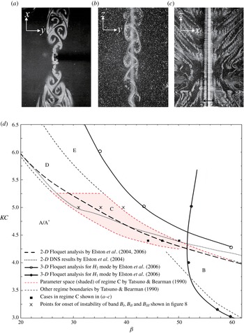
(a–c) Experimental visualisations of streaklines at
 $KC=4.4$
and different
 $\unicode[STIX]{x1D6FD}$
numbers, where the oscillation of the cylinder was in the
 $x$
-direction, reproduced from Tatsuno & Bearman (Reference Tatsuno and Bearman1990) at (a)
 $\unicode[STIX]{x1D6FD}=44.2$
, (b) 46.9 and (c) 50.1. The length of the cylinder normalised by its diameter in the test was
 $L_{z}\approx 12.1\unicode[STIX]{x03C0}$
. (d) The location of regime C flow as indicated by the shaded area, along with the boundaries of different flow regimes classified by Tatsuno & Bearman (Reference Tatsuno and Bearman1990) and numerically reproduced by Elston, Sheridan & Blackburn (Reference Elston, Sheridan and Blackburn2004) and Elston et al. (Reference Elston, Blackburn and Sheridan2006).

Among the aforementioned regimes, the mechanisms for the initiation and development of regime C flow are not fully understood. Regime C flow is characterised by fascinating flow patterns, as illustrated in figure 1 at
 $KC=4.4$
by dye streaklines (Tatsuno & Bearman Reference Tatsuno and Bearman1990). At
 $\unicode[STIX]{x1D6FD}=44.2$
, figure 1(a) shows that the dye sheets shed during the cylinder roll up to form large vortices associated with a distinctive secondary period on the
 $(x,y)$
-plane that is parallel to the oscillation axis. These vortices are arranged similarly to a von Kármán vortex street behind a cylinder in the uniform flow, only in an opposite sense of rotation. At
 $\unicode[STIX]{x1D6FD}=46.9$
, figure 1(b) shows a
 $(y,z)$
-plane view where sinusoidal flapping of oblique directions of vortex flow in the spanwise direction is observed. At
 $\unicode[STIX]{x1D6FD}=50.1$
, figure 1(c) shows an
 $(x,z)$
-plane view where large-scale vortices emanate away from the cylinder axis. In addition, the emanation directions appear to be different across the span of the cylinder, forming the shape of an X in the dye sheet arrangement and hence named the X-mode. This pattern is not unique to planar oscillatory flows as it was also found in an elliptical oscillatory flow around a circular cylinder, as reported by Yang & Rockwell (Reference Yang and Rockwell2002), in which the spanwise vortex shedding mode at
 $KC=10$
is particularly similar to the regime C flow. Note that the
 $KC$
number reported in Yang & Rockwell (Reference Yang and Rockwell2002) was defined by the wave orbital velocity magnitude on the free surface; thus, it is not directly comparable with the
 $KC$
reported in this study.
Tatsuno & Bearman (Reference Tatsuno and Bearman1990) also experimentally determined the regime boundaries in the (
 $KC,\unicode[STIX]{x1D6FD}$
)-space, as reproduced in figure 1(d). The regime C flow only appears in a confined range within
 $4.3\leqslant KC\leqslant 5.2$
and
 $27\leqslant \unicode[STIX]{x1D6FD}\leqslant 53$
. The regime C flow was further investigated by Elston et al. (Reference Elston, Sheridan and Blackburn2004, Reference Elston, Blackburn and Sheridan2006) through Floquet stability analysis and direct numerical simulations (DNS). The predicted regime boundaries (or marginal stability curves) between regime A and regime D are also presented in figure 1(d), which agree well with the experimental result. However, clear discrepancies exist among the boundaries that separate regime A and regime C. Specifically, the difference between the results of 2-D DNS and Floquet analysis (Elston et al.
Reference Elston, Sheridan and Blackburn2004) is somewhat unexpected. The reason for this difference is unclear. In addition, the regime boundaries obtained by using 2-D DNS and Floquet analysis lie above those obtained experimentally. Elston et al. (Reference Elston, Blackburn and Sheridan2006) extended their 2-D work to 3-D Floquet analysis and 3-D DNS. Two additional branches of 3-D marginal stability curves were reported, as shown in figure 1(d). The upper branch is located above the 2-D marginal curves, and the lower branch intersects with the 2-D marginal stability curves. The lower branch has
 $H_{1}$
spatio-temporal symmetry with a spanwise wavenumber of
 $k=2\unicode[STIX]{x03C0}/\unicode[STIX]{x1D706}$
ranging from 2.9 to 6.6, where
 $\unicode[STIX]{x1D706}$
is the spanwise wavelength, whereas the upper branch has
 $H_{2}$
symmetry with
 $k$
ranging from 4.6 to 8.2. Here, the
 $H_{1}$
and
 $H_{2}$
symmetries are defined as
 $$\begin{eqnarray}\displaystyle & \displaystyle H_{1}:(u,v,w)(x,y,z,t)=(-u,v,w)(-x,y,z,t+T/2), & \displaystyle\end{eqnarray}$$
 $$\begin{eqnarray}\displaystyle & \displaystyle H_{2}:(u,v,w)(x,y,z,t)=(-u,-v,w)(-x,-y,z,t+T/2). & \displaystyle\end{eqnarray}$$
The lower branch generally agrees well with the experimental regime boundary between regime
 $\text{A}^{\ast }$
and regime B. In addition, the experimental and numerical observations of the Honji instability (Honji Reference Honji1981; An, Cheng & Zhao Reference An, Cheng and Zhao2011) confirmed that regime B flow has
 $H_{1}$
symmetry at any cross-sectional plane. However, the physical meaning of the upper branch (the
 $H_{2}$
mode) is not well understood, primarily because the base flow is artificially constrained to be
 $K_{x}$
symmetric while the flow in practice at these parameters is in regime E according to the experimental results (Tatsuno & Bearman Reference Tatsuno and Bearman1990). The 3-D DNS results obtained by Elston et al. (Reference Elston, Blackburn and Sheridan2006) also suggested that flow in regime C is initially unstable to a band of wavenumbers that emanate from
 $k=0$
. The iso-surface of spanwise vorticity from the simulation at
 $(\unicode[STIX]{x1D6FD},KC,k)=(40,4.8,0.5)$
is consistent with the spanwise flapping and slantwise vortex shedding pattern, as shown in figure 1(b,c).
Dütsch et al. (Reference Dütsch, Durst, Becker and Lienhart1998) performed a 2-D numerical simulation at
 $\unicode[STIX]{x1D6FD}=35$
and decomposed the inline force on the circular cylinder into drag and inertia components according to the Morison equation. At
 $KC=5$
, where the flow belongs to regime C, the drag coefficient
 $C_{D}$
agrees well with the experimental results reported by Kuehtz (Reference Kuehtz1996), and the predicted inertia coefficient
 $C_{M}$
is only slightly lower than the experimental value. The good agreement between the 2-D numerical results and the experimental data suggests that the three-dimensionality of regime C flow has limited influence on the inline forces. Yang & Rockwell (Reference Yang and Rockwell2002) experimentally studied the spanwise flow patterns induced by wave interactions with a circular cylinder in a wave tank, where the fluid particles move in elliptical trajectories. The vortex shedding along the span of the cylinder exhibits a sinuous phase variation and thus forms a pattern of S at both low and moderate
 $KC$
numbers, which is named the S-mode. This mode involves large-scale distortions in flow patterns, which are characterised by variations in transverse velocity and streamwise vorticity with a wavelength in the range
 $1\leqslant \unicode[STIX]{x1D706}/D\leqslant 4.5$
at small
 $KC$
values or
 $10\leqslant \unicode[STIX]{x1D706}/D\leqslant 110$
at moderate
 $KC$
values. As mentioned above, this phenomenon is very similar to the observation of flow patterns in regime C by Tatsuno & Bearman (Reference Tatsuno and Bearman1990).
Nehari et al. (Reference Nehari, Armenio and Ballio2004) conducted a numerical study of 3-D flow features in regimes D and F. At
 $(KC,\unicode[STIX]{x1D6FD})=(6.5,20)$
in regime D, intermittent switching of oblique vortex shedding directions from one side of the oscillation axis to the other was observed in both 2-D and 3-D simulations, which is slightly different from the results reported by Tatsuno & Bearman (Reference Tatsuno and Bearman1990) that the direction of the transverse vortex street with this parameter set remains stationary. The total inline force acting on the cylinder and the sectional inline force are only weakly affected by the three-dimensionality of the flow, whereas the influence of flow three-dimensionality on the lift (or transverse force,
 $F_{y}$
) is apparent. In addition, the spanwise variation in the sectional transverse force is much larger than the variation in the inline force. This observation is supported by the flow features of the S-mode observed by Yang & Rockwell (Reference Yang and Rockwell2002).
The three-dimensional characteristics of regime C flows are not yet fully understood, which is possibly due to the difficulties associated with physically visualising and numerically modelling the flow. The present study aims to investigate the following aspects of the regime C flow:
(i) the onset conditions of 3-D instability,
(ii) three-dimensional flow fields and the physics behind the 3-D vortex patterns,
(iii) the intrinsic link between vortex patterns and spanwise modulations of the forces on the cylinder and
(iv) the physical mechanisms responsible for the discrepancy in the marginal stability curves obtained from the linear stability analysis and the experiments.
This numerical investigation consists of 2-D and 3-D Floquet analyses and DNS. The remainder of this paper is organised in the following manner: § 2 briefly introduces the numerical models for the Floquet analysis and DNS, the results and discussions are presented in § 3 and concluding remarks are provided in § 4. Model validation on the numerical approaches is demonstrated in the Appendix.
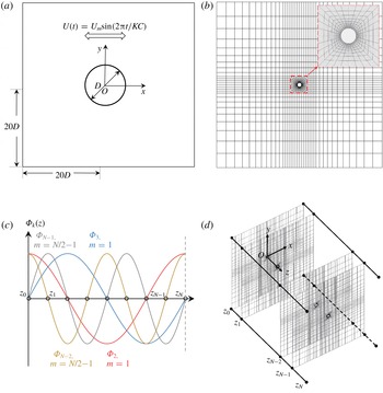
Illustrations of the physical problem and numerical implementation. (a) Schematic representation of the problem. (b) The distribution of the 2-D
 $h$
-type mesh in the
 $(x,y)$
-plane, along with a close-up view of the
 $hp$
-refined mesh around the cylinder at Lagrange interpolate order
 $N_{p}=8$
. (c) The demonstration of the corresponding Fourier basis employed by the Fourier spectral/
 $hp$
method. (d) The definition of the three-dimensional coordinate system and spanwise discretisation in the physical space after inverse Fourier transformation.

2 Numerical method
The focus of this study is the flow induced by an oscillating cylinder in still water with a given frequency and amplitude, as illustrated in figure 2. The origin of the oscillating reference frame is fixed at the centre of the circular cylinder, and its axes are referred to as
 $(x,y)$
. The size of the 2-D computational domain is
 $40D\times 40D$
, which was deemed to be adequate for the flow within the parameter space covered in this study according to Elston et al. (Reference Elston, Blackburn and Sheridan2006). The dimensionless unsteady Navier–Stokes (N–S) equations, which govern the flow, are expressed in the following form:
 $$\begin{eqnarray}\displaystyle & \displaystyle {\displaystyle \frac{\unicode[STIX]{x2202}\boldsymbol{u}}{\unicode[STIX]{x2202}t}}=-(\boldsymbol{u}\boldsymbol{\cdot }\unicode[STIX]{x1D735})\boldsymbol{u}-\unicode[STIX]{x1D735}p+Re^{-1}\unicode[STIX]{x1D6FB}^{2}\boldsymbol{u}+\boldsymbol{i}_{x}\unicode[STIX]{x1D714}\text{cos}(\unicode[STIX]{x1D714}t), & \displaystyle\end{eqnarray}$$
 $$\begin{eqnarray}\displaystyle & \displaystyle \unicode[STIX]{x1D735}\boldsymbol{\cdot }\boldsymbol{u}=0, & \displaystyle\end{eqnarray}$$
where
 $\boldsymbol{u}$
is the velocity vector,
 $p$
is the pressure field and
 $\boldsymbol{i}_{x}$
is the unit vector in the streamwise direction, acting as the direction vector of inertia force. The velocity components
 $u$
and
 $v$
are in the
 $x$
- and
 $y$
-directions, respectively. The spanwise velocity,
 $w$
, is applicable to three-dimensional simulations. The velocity components are normalised by the amplitude (
 $U_{m}$
) of the oscillation velocity, and the axes are normalised by the cylinder diameter
 $D$
.
For 2-D DNS, the above N–S equations are solved by an extensively validated spectral/
 $hp$
element method embedded in Nektar++ (Cantwell et al.
Reference Cantwell, Moxey, Comerford, Bolis, Rocco, Mengaldo, De Grazia, Yakovlev, Lombard, Ekelschot, Jordi, Xu, Mohamied, Eskilsson, Nelson, Vos, Biotto, Kirby and Sherwin2015). The same boundary conditions as those employed by Elston et al. (Reference Elston, Blackburn and Sheridan2006) are adopted and described briefly here. The velocity of the oscillating cylinder is specified as
 $U(t)=U_{m}\text{sin}(2\unicode[STIX]{x03C0}t/KC)$
and
 $V=0$
on the far-field boundaries of the computational domain because the reference frame moves with the cylinder. Consequently, zero Dirichlet velocity boundary conditions are applied on the cylinder surface. A high-order Neumann pressure boundary condition is adopted on all domain boundaries, as described by Blackburn & Henderson (Reference Blackburn and Henderson1999). Initial conditions of zero flow velocity superposed with random perturbations of
 $10^{-5}$
and pressure are employed in the simulations unless specified otherwise.
Floquet stability analysis is performed on the same 2-D mesh to investigate the 2-D and 3-D instabilities. This part can be considered an extension of the work reported by Elston et al. (Reference Elston, Blackburn and Sheridan2006) on regime C with the same numerical approach, which is not detailed here. Briefly, we intend to solve an eigenvalue problem from the linearised continuity and N–S equations. Floquet analysis examines the evolution of infinitesimal perturbations according to these linearised equations based on a
 $T$
-periodic base flow,
 $\boldsymbol{U}$
. The Floquet multiplier
 $\unicode[STIX]{x1D707}=\text{exp}(\unicode[STIX]{x1D70E}T\pm \text{i}\unicode[STIX]{x1D714}_{s}T)$
is the eigenvalue used to identify the instability of the flow, where
 $\unicode[STIX]{x1D70E}$
and
 $\unicode[STIX]{x1D714}_{s}$
denote the exponential growth rate and angular frequency. Instability occurs when
 $\unicode[STIX]{x1D70E}>0$
(perturbation increases exponentially), whereas stability is indicated by
 $\unicode[STIX]{x1D70E}<0$
(perturbation decays exponentially). The Floquet multipliers for the transition between regime A and regime C occur in complex-conjugate pairs
 $\unicode[STIX]{x1D707}=|\unicode[STIX]{x1D707}|\text{exp}(\pm \text{i}\unicode[STIX]{x1D714}_{s}T)=|\unicode[STIX]{x1D707}|\text{cos}(\unicode[STIX]{x1D714}_{s}T)\pm i|\unicode[STIX]{x1D707}|\text{sin}(\unicode[STIX]{x1D714}_{s}T)$
(Elston et al.
Reference Elston, Blackburn and Sheridan2006), where the magnitude of the Floquet multiplier is
 $|\unicode[STIX]{x1D707}|=\text{exp}(\unicode[STIX]{x1D70E}T)$
. The angular frequency
 $\unicode[STIX]{x1D714}_{s}$
is related to a new secondary period as
 $T_{s}/T=2\unicode[STIX]{x03C0}/\unicode[STIX]{x1D714}_{s}$
, or the normalised secondary frequency
 $f_{s}T=\unicode[STIX]{x1D714}_{s}/2\unicode[STIX]{x03C0}$
, leading to a quasi-periodic state in regime C. A series of Floquet multipliers are obtained at a given pair of
 $KC$
and
 $\unicode[STIX]{x1D6FD}$
over a range of spanwise wavenumbers
 $k$
. The general perturbations are expressed as a Fourier integral of eigenfunctions
 $\hat{\boldsymbol{u}}_{k}^{c}$
and
 $\hat{\boldsymbol{u}}_{k}^{s}$
throughout all wavenumbers
 $k$
,
 $$\begin{eqnarray}\displaystyle & \displaystyle \widetilde{\boldsymbol{u}}(x,y,z,t)=\int _{-\infty }^{\infty }[\hat{\boldsymbol{u}}_{k}^{c}(x,y,t)\text{cos}(2k\unicode[STIX]{x03C0}z)+\hat{\boldsymbol{u}}_{k}^{s}(x,y,t)\text{sin}(2k\unicode[STIX]{x03C0}z)]. & \displaystyle\end{eqnarray}$$
The spanwise wavenumber
 $k$
corresponds to the wavelength
 $\unicode[STIX]{x1D706}$
of the perturbation as
 $\unicode[STIX]{x1D706}=2\unicode[STIX]{x03C0}/k$
. Because modes with different
 $k$
values do not couple in the linear analysis, the Floquet multiplier for each
 $k$
can be obtained individually via subspace iterations. The iteration is performed on a Krylov subspace of 16 dimensions, initialised from a random starting vector. The leading eigenvalue and eigenmode are obtained by applying the above operation on a range of
 $k$
values.
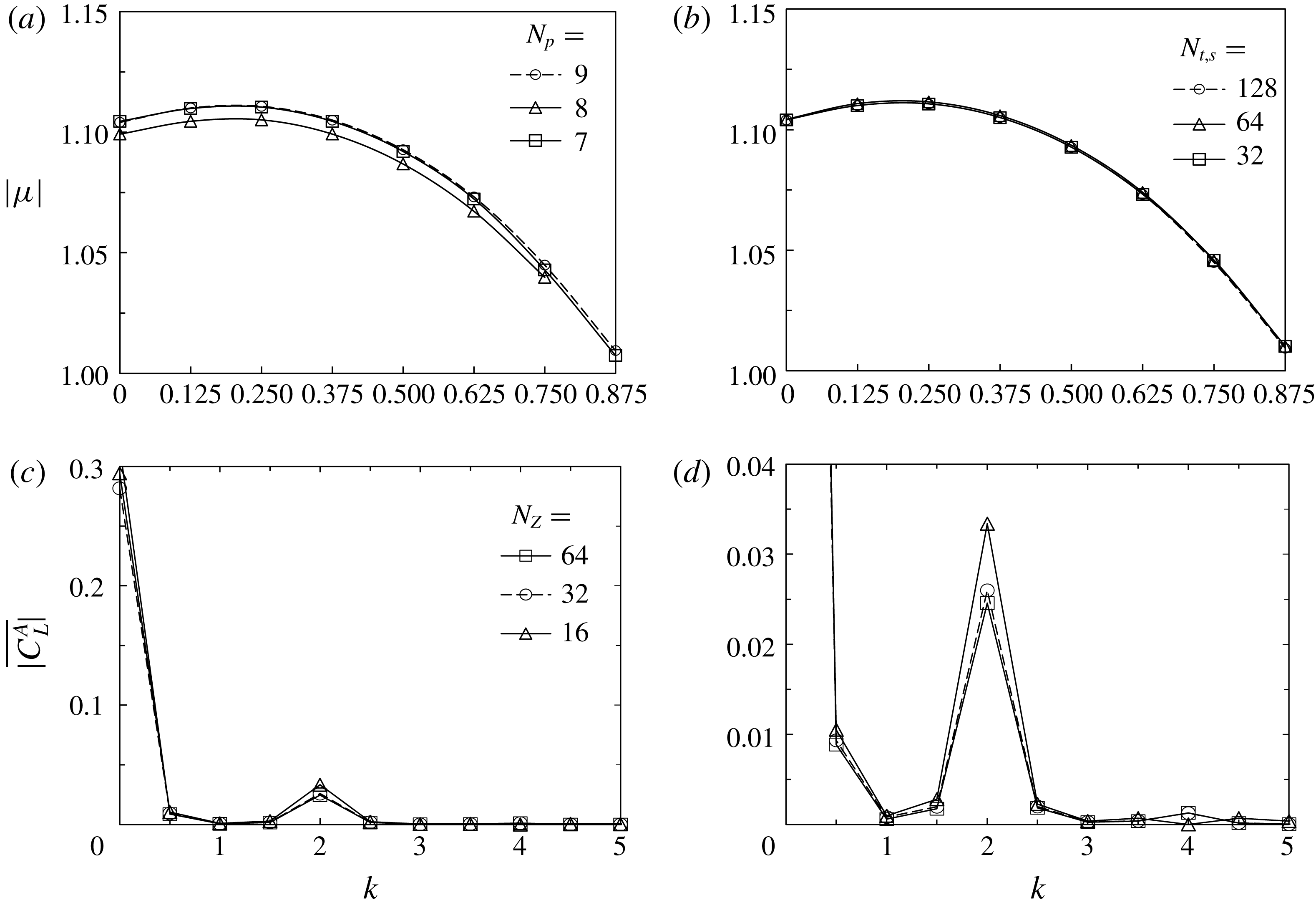
The 2-D mesh distribution adopted in the present study is shown in figure 2(b). The dependence of the numerical results on the Lagrange interpolant order
 $N_{p}$
is studied and presented in the Appendix. Specifically,
 $N_{p}=8$
is selected for both DNS and Floquet analysis in this study. A total of 256 azimuthal mesh points are uniformly distributed on the circular cylinder surface, and the size of the first layer grid from the cylinder surface is less than
 $0.01D$
, which is slightly smaller than that used in Elston et al. (Reference Elston, Blackburn and Sheridan2006). A time Fourier interpolation method is adopted to reconstruct the base flow
 $\boldsymbol{U}$
based on the data from
 $N_{t.s}=64$
time slices, which are equi-spaced in one period
 $T$
of flow oscillations. The dependence of the numerical results on
 $N_{t.s}$
is also evaluated and presented in the Appendix.
A quasi-3-D approach, where a spectral/
 $hp$
element method is employed to discretise the problem in the
 $(x,y)$
-plane with the same mesh as that used in the 2-D simulation and a Fourier discretisation is implemented in the
 $z$
-direction to resolve the full 3-D features of the flow, is used to solve the three-dimensional N–S equations (Karniadakis Reference Karniadakis1990). Hence, only a 2-D mesh is required for this quasi-3-D approach. One can refer to Bolis (Reference Bolis2013) for more details about this technique and its implementation in Nektar++. In general, the velocity vector and pressure are expressed as Fourier expansions:
 $$\begin{eqnarray}\displaystyle & \displaystyle \boldsymbol{u}(x,y,z,t)=\mathop{\sum }_{m=0}^{N_{z}/2-1}\left[\hat{\boldsymbol{u}}_{m}^{c}(x,y,t)\text{cos}\left({\displaystyle \frac{2m\unicode[STIX]{x03C0}z}{L_{z}}}\right)+\hat{\boldsymbol{u}}_{m}^{s}(x,y,t)\text{sin}\left({\displaystyle \frac{2m\unicode[STIX]{x03C0}z}{L_{z}}}\right)\right], & \displaystyle\end{eqnarray}$$
 $$\begin{eqnarray}\displaystyle & \displaystyle p(x,y,z,t)=\mathop{\sum }_{m=0}^{N_{z}/2-1}\left[\hat{p}_{m}^{c}(x,y,t)\text{cos}\left({\displaystyle \frac{2m\unicode[STIX]{x03C0}z}{L_{z}}}\right)+\hat{p}_{m}^{s}(x,y,t)\text{sin}\left({\displaystyle \frac{2m\unicode[STIX]{x03C0}z}{L_{z}}}\right)\right], & \displaystyle\end{eqnarray}$$
where each velocity component of Fourier modes
 $\hat{\boldsymbol{u}}_{m}^{c}$
(cosine part) and
 $\hat{\boldsymbol{u}}_{m}^{s}$
(sine part) is a three-dimensional velocity vector field, containing
 $(u,v,w)$
components at any Fourier order
 $m$
ranging from
 $m=0$
(2-D component) to
 $N_{z}/2-1$
with a corresponding Fourier basis
 $$\begin{eqnarray}\displaystyle & \displaystyle \unicode[STIX]{x1D6F7}_{2m}=\text{cos}\left({\displaystyle \frac{2m\unicode[STIX]{x03C0}z}{L_{z}}}\right)\quad \text{and} & \displaystyle\end{eqnarray}$$
 $$\begin{eqnarray}\displaystyle & \displaystyle \unicode[STIX]{x1D6F7}_{2m+1}=\text{sin}\left({\displaystyle \frac{2m\unicode[STIX]{x03C0}z}{L_{z}}}\right), & \displaystyle\end{eqnarray}$$
respectively (figure 2
c). Here,
 $N_{z}$
represents the spanwise resolution of the simulation because the inverse Fourier transform would yield the flow field
 $\boldsymbol{u}(x,y,z_{i},t)$
at
 $z=z_{i}$
for
 $i=0,1,\ldots ,N_{z}-1$
(figure 2
d). The Fourier mode at
 $m$
corresponds to a 3-D instability with a wavelength of
 $\unicode[STIX]{x1D706}=L_{z}/m$
or wavenumber
 $k=2\unicode[STIX]{x03C0}m/L_{z}$
.
Linear operators are applied to each component separately, and a coupling algorithm is employed to address the nonlinear part when solving the N–S equations. Apart from the periodic boundary condition enforced on the lateral boundaries that are perpendicular to the cylinder, the other boundary conditions are the same as those specified in the 2-D simulation where spanwise velocity
 $w=0$
. The Fourier expansion of pressure can be explained in the same manner as described above and is thus omitted here.
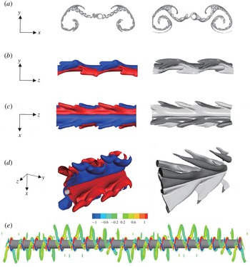
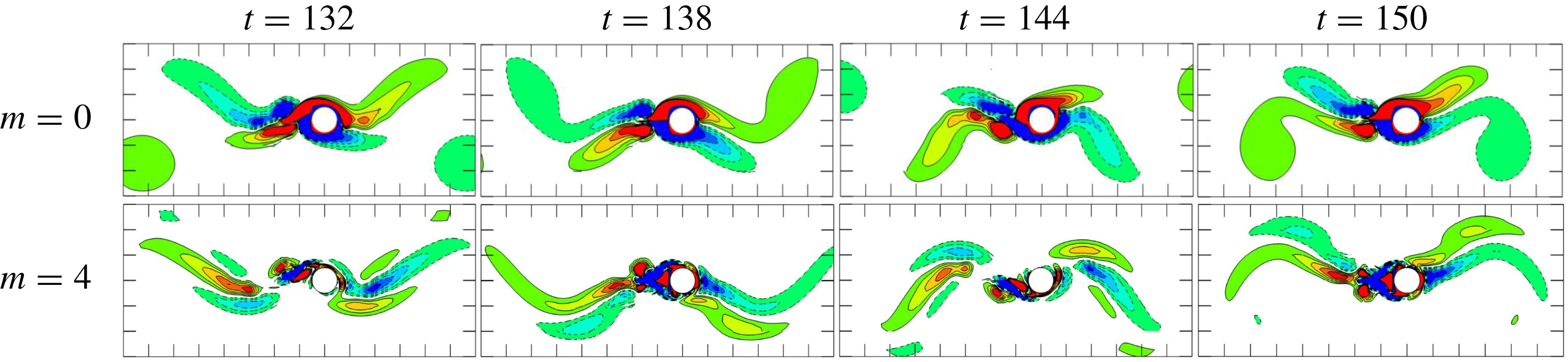
Comparison of flow visualisations between the present study (left) and published numerical results (right). (a) Streaklines of flow at
 $(KC,\unicode[STIX]{x1D6FD})=(5,36)$
, compared with Tong et al. (Reference Tong, Cheng, Zhao and An2015). (b–d) Instantaneous iso-surfaces of vorticity, compared with Elston et al. (Reference Elston, Blackburn and Sheridan2006). (e) Sectional slices of spanwise vorticity
 $\unicode[STIX]{x1D714}_{z}$
at
 $(KC,\unicode[STIX]{x1D6FD})=(4.8,40,0.5)$
.

Some of the flow visualisation results from the 2-D and 3-D DNS are compared with the published numerical results in figure 3. The 2-D streakline pattern at
 $(KC,\unicode[STIX]{x1D6FD})=(5,36)$
in figure 3(a) agrees well with that of Tong et al. (Reference Tong, Cheng, Zhao and An2015) shown on the right. The 3-D simulation results of an iso-surface of the spanwise vorticity are compared with the 3-D DNS results at
 $(KC,\unicode[STIX]{x1D6FD})=(4.8,40,0.5)$
(Elston et al.
Reference Elston, Blackburn and Sheridan2006). Although there are some subtle differences between the iso-surfaces, the three-dimensional vortex features are very similar. A sinuous switch of oblique direction along the span of the cylinder is observed from the side view in figure 3(b) and in the cross-sectional slices shown in figure 3(e). The top view in figure 3(c) presents a V-pattern. The slantwise vortex shedding is shown in the perspective view in figure 3(d).
3 Results and discussion
3.1 Stability analysis
The purpose of the Floquet stability analysis is to
(i) resolve the disparity in predicting the transition boundary between regime A and regime C by the 2-D Floquet analysis and the experimental observations, as illustrated in figure 1, and
(ii) investigate the 3-D instabilities associated with low wavenumbers, which cannot easily be resolved using 3-D DNS due to the requirement of a large spanwise domain size. The study presented in this section can be considered to be complementary to the work by Elston et al. (Reference Elston, Blackburn and Sheridan2006), where the focus was largely on 3-D instabilities with relatively high wavenumbers.
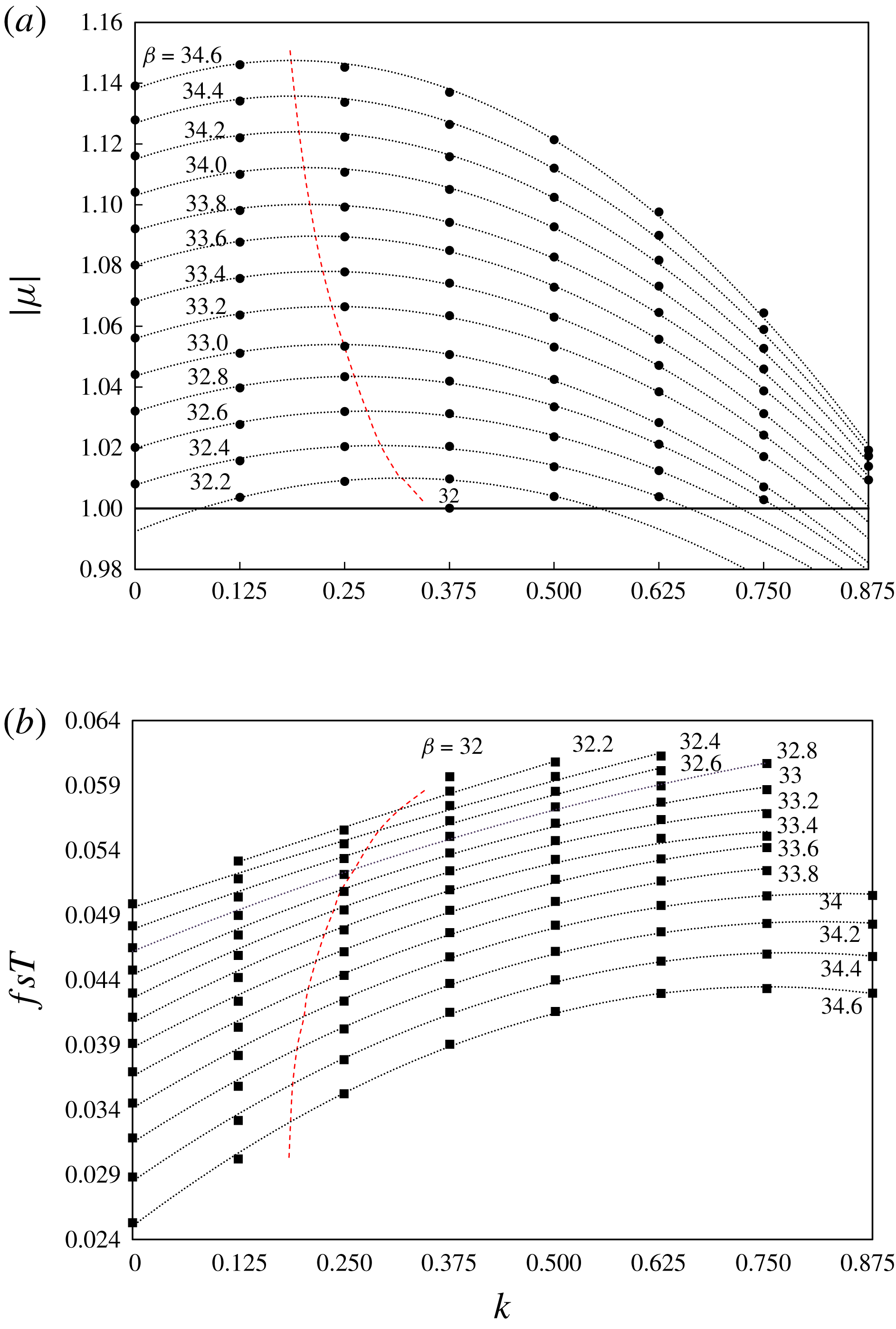
(a) Floquet multiplier with respect to different wavenumbers
 $k$
at
 $KC=5$
and (b) the corresponding normalised secondary frequency
 $f_{s}T=\unicode[STIX]{x1D703}/2\unicode[STIX]{x03C0}$
. The symbols indicate the simulated cases, and the dotted lines are curve fits using a parabolic function. The trend line of the leading instability is denoted by the dashed lines.

(a) Comparison of
 $\unicode[STIX]{x1D714}_{z}$
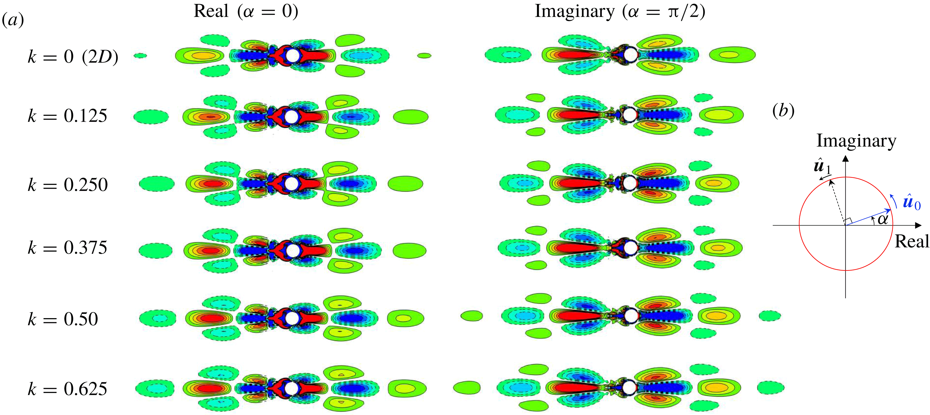
vorticity contours of the Floquet eigenmodes and (b) diagram of the phase variation in a pair of Floquet eigenmodes. Both the real and imaginary parts of the Floquet eigenmodes associated with a pair of complex-conjugate Floquet multipliers are shown for different wavenumbers (
 $k$
) at
 $(KC,\unicode[STIX]{x1D6FD})=(5,32.4)$
. Each vorticity contour is normalised by the average magnitude
 $\unicode[STIX]{x1D714}_{z}^{\ast }=\unicode[STIX]{x1D714}_{z}/\overline{|\unicode[STIX]{x1D714}_{z}|}$
.

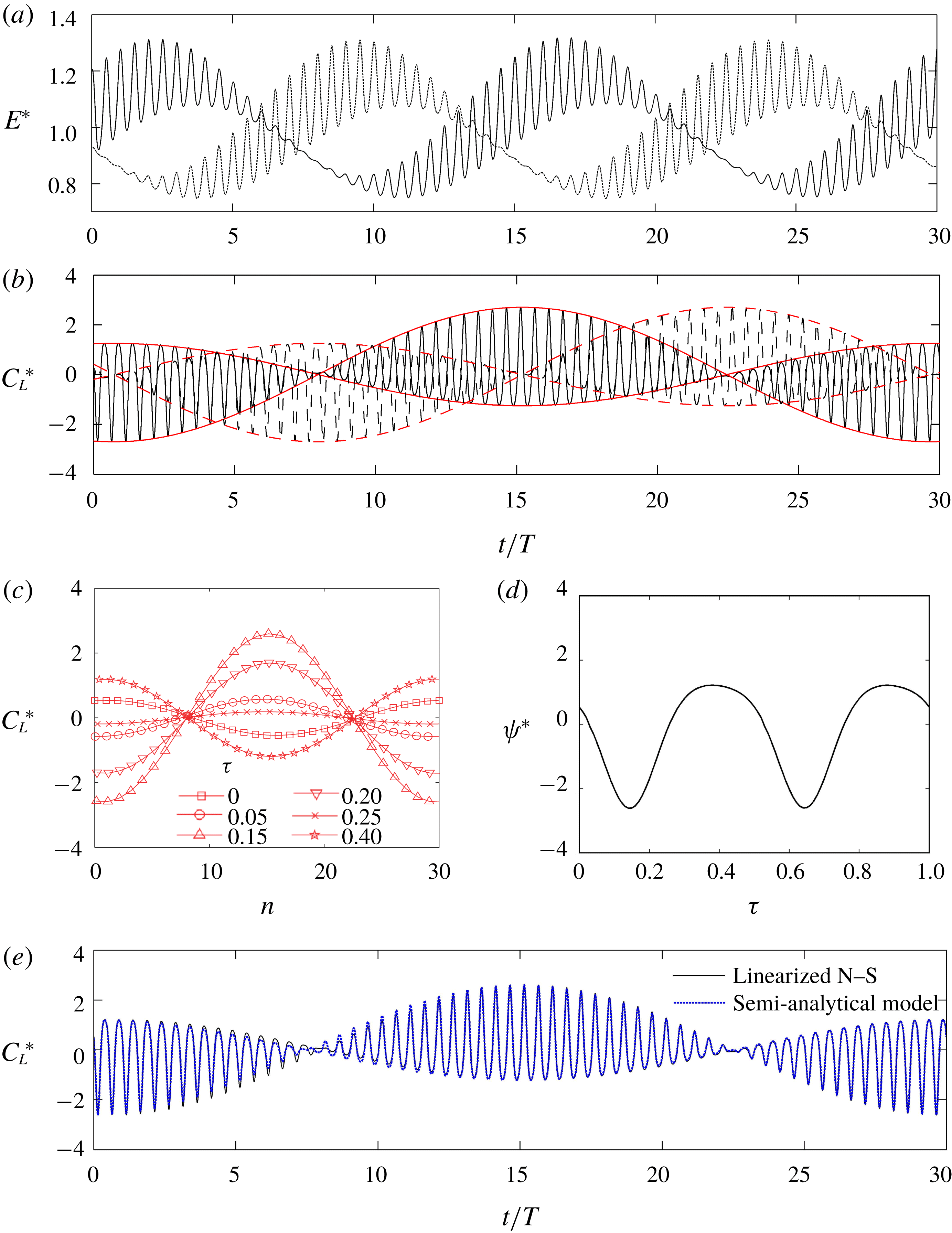
The phase variation in (a) normalised energy and (b) lift coefficient at
 $(KC,\unicode[STIX]{x1D6FD},k)=(5,34,0)$
of a pair of eigenmodes by the linearised N–S equation, where the Floquet multiplier is
 $|\unicode[STIX]{x1D707}|=1.104$
and the normalised secondary frequency is
 $f_{s}T=0.0345$
(
 $T_{s}/T=28.99$
): ——, for
 $\hat{\boldsymbol{u}}_{\mathbf{0}}$
; - - - -, for
 $\hat{\boldsymbol{u}}_{\mathbf{1}}$
; —— (red) and - - - - (red), for the envelope curve for the trace of lift coefficient. (c) The temporal variation in lift coefficient at each fixed phase of streamwise oscillation (
 $\unicode[STIX]{x1D70F}$
). (d) The function of amplitude
 $\unicode[STIX]{x1D6F9}^{\ast }$
with respect to phase variation. (e) Comparison of instantaneous lift coefficient between the result from the linearised N–S and the proposed semi-analytical model for the same case.

Figure 4 presents the variations in the Floquet multiplier and the normalised secondary frequency with wavenumber for flows at
 $KC=5$
. The base flow for the 3-D analysis is obtained with the same approach as in the 2-D Floquet analysis. The 3-D instabilities with very low wavenumbers are examined. The results suggest that the base flow is initially unstable against 3-D instabilities with
 $k=0.375$
at
 $\unicode[STIX]{x1D6FD}=32.0$
. As
 $\unicode[STIX]{x1D6FD}$
increases,
 $|\unicode[STIX]{x1D707}|>1$
at different unstable wavenumbers form a concave down shape. The wavenumber with the largest Floquet multiplier decreases with increasing
 $\unicode[STIX]{x1D6FD}$
, as indicated by the dashed line in figure 4. The unstable eigenmodes are quasi-periodic because the corresponding Floquet multiplier is a complex number. The secondary period (or frequency) is calculated from the angle of the complex Floquet multiplier, as shown in figure 4(b). The secondary frequency (
 $f_{s}$
) of the unstable eigenmode decreases with increasing
 $\unicode[STIX]{x1D6FD}$
, which agrees with the results reported by (Elston et al.
Reference Elston, Blackburn and Sheridan2006). However, at a constant
 $\unicode[STIX]{x1D6FD}$
, the frequency monotonically increases with
 $k$
, indicating possible temporal modulations of eigenmodes of different wavenumbers at different frequencies.
Figure 5(a) shows the eigenmodes for each
 $k$
in the range of 0 (2-D) to 0.625 with an interval of 0.125 at
 $(KC,\unicode[STIX]{x1D6FD})=(5,32.4)$
. Since the Floquet eigenmodes are obtained through an iteration method in which the perturbation flow field has to be normalised in each iteration, the strength of the vorticity in each plot does not necessarily reflect the amplitude of the corresponding eigenvalue (Floquet multiplier). Moreover, as shown in figure 5(b), the eigenmodes of a pair of complex conjugate Floquet multipliers shift along a circular path in the complex space with an angular frequency of
 $\unicode[STIX]{x1D714}_{s}=2\unicode[STIX]{x03C0}f_{s}$
(phase angle of the secondary period
 $\unicode[STIX]{x1D6FC}=2\unicode[STIX]{x03C0}f_{s}t$
) with a phase lag of
 $\unicode[STIX]{x03C0}/2$
. The eigenmode at phase
 $\unicode[STIX]{x1D6FC}=2\unicode[STIX]{x03C0}f_{s}(nT)$
is dependent on the number of iterations
 $n$
needed for the Floquet multiplier to reach convergence tolerance (
 $10^{-7}$
). Therefore, the phase
 $\unicode[STIX]{x1D6FC}$
at the end of each iteration for different
 $k$
is arbitrary and thus not necessarily the same. For this reason, the eigenmodes for the band of low-wavenumber instabilities (
 $k<1$
) are actually very similar to each other. Although the vorticity fields break the
 $K_{x}$
symmetry, they all possess inverse
 $K_{x}$
symmetry, which is defined as
 $\unicode[STIX]{x1D714}_{z}(x,y,z,t)=\unicode[STIX]{x1D714}_{z}(x,-y,z,t)$
. This leads to a non-zero transverse force due to the net circulation around the cylinder.
Temporal variations in the instantaneous energy of the instability and lift coefficient over one secondary period induced by a pair of eigenmodes are further examined by solving the standard linearised N–S equations of perturbations with the same base flow as that used in the Floquet analysis and the eigenmode as initial conditions, and the results are shown in figure 6(a,b). The instantaneous energy
 $E$
of the instability is calculated as
 $$\begin{eqnarray}\displaystyle & \displaystyle E=\int _{\unicode[STIX]{x1D6FA}}\Vert \hat{\boldsymbol{u}}\Vert ^{2}\,\text{d}\unicode[STIX]{x1D6FA}. & \displaystyle\end{eqnarray}$$
The instantaneous lift coefficient
 $C_{L}$
on a unit length cylinder is defined as
 $C_{L}=F_{y}/(1/2\unicode[STIX]{x1D70C}DU^{2})$
, where
 $F_{y}$
is the transverse force experienced by the cylinder. The effect of exponential growth is eliminated through the following normalisation:
 $$\begin{eqnarray}\displaystyle & \displaystyle E^{\ast }=E^{\prime }/\overline{E^{\prime }},\quad E^{\prime }=E/G^{2}, & \displaystyle\end{eqnarray}$$
 $$\begin{eqnarray}\displaystyle & \displaystyle C_{L}^{\ast }=C_{L}^{\prime }/(C_{L}^{\prime })_{std},\quad C_{L}^{\prime }=C_{L}/G, & \displaystyle\end{eqnarray}$$
 $$\begin{eqnarray}\displaystyle & \displaystyle \hat{\boldsymbol{u}}_{0}^{\ast }=\hat{\boldsymbol{u}}_{0}/G, & \displaystyle\end{eqnarray}$$
 $$\begin{eqnarray}\displaystyle & \displaystyle G=|\unicode[STIX]{x1D707}|^{t/T}, & \displaystyle\end{eqnarray}$$
where
 $G=|\unicode[STIX]{x1D707}|^{t/T}$
is the exponential growth and
 $(.)_{std}$
denotes the operator for the standard deviations. Both
 $E^{\ast }$
and
 $C_{L}^{\ast }$
vary at two distinct frequencies: one is associated with the streamwise oscillation frequency (or period) with a phase of
 $\unicode[STIX]{x1D70F}=t/T-n$
, where
 $n=\lfloor t/T\rfloor$
is the sequence number of the streamwise oscillation, and the other is associated with the secondary frequency with a phase of
 $\unicode[STIX]{x1D6FC}=2\unicode[STIX]{x03C0}f_{s}t+\unicode[STIX]{x1D6FC}_{0}$
, where
 $\unicode[STIX]{x1D6FC}_{0}$
is the initial phase. In addition, an obvious phase lag of
 $\unicode[STIX]{x03C0}/2$
exists between the secondary oscillations of
 $\hat{\boldsymbol{u}}_{0}$
and
 $\hat{\boldsymbol{u}}_{1}$
, as illustrated in figure 5. The variation trend of
 $C_{L}^{\ast }$
is further analysed by separating the variables as follows:
 $$\begin{eqnarray}\displaystyle & \displaystyle C_{L}^{\ast }=\unicode[STIX]{x1D6F9}^{\ast }(\unicode[STIX]{x1D70F})\text{cos}(\unicode[STIX]{x1D6FC}), & \displaystyle\end{eqnarray}$$
where the function
 $\unicode[STIX]{x1D6F9}^{\ast }$
represents the phase variation associated with the streamwise oscillation and
 $\text{cos}(\unicode[STIX]{x1D6FC})$
represents the modulation by the secondary frequency. The function
 $\unicode[STIX]{x1D6F9}^{\ast }$
is determined from the temporal variation in
 $C_{L}^{\ast }$
at each fixed phase of streamwise oscillation (
 $\unicode[STIX]{x1D70F}$
) (figure 6
c,d). The normalised lift coefficient at a fixed phase
 $\unicode[STIX]{x1D70F}$
of streamwise oscillation varies with the number of cycles of oscillation
 $n=t/T-\unicode[STIX]{x1D70F}$
.
 $\unicode[STIX]{x1D6F9}^{\ast }$
is a function of phase
 $\unicode[STIX]{x1D70F}$
and peaks at
 $\unicode[STIX]{x1D70F}\approx 0.15$
and 0.65. A comparison of the instantaneous
 $C_{L}^{\ast }$
obtained by the linearised simulations and by (3.6) is shown in figure 6(e). The variation in the instantaneous
 $C_{L}^{\ast }$
is characterised well by (3.6).
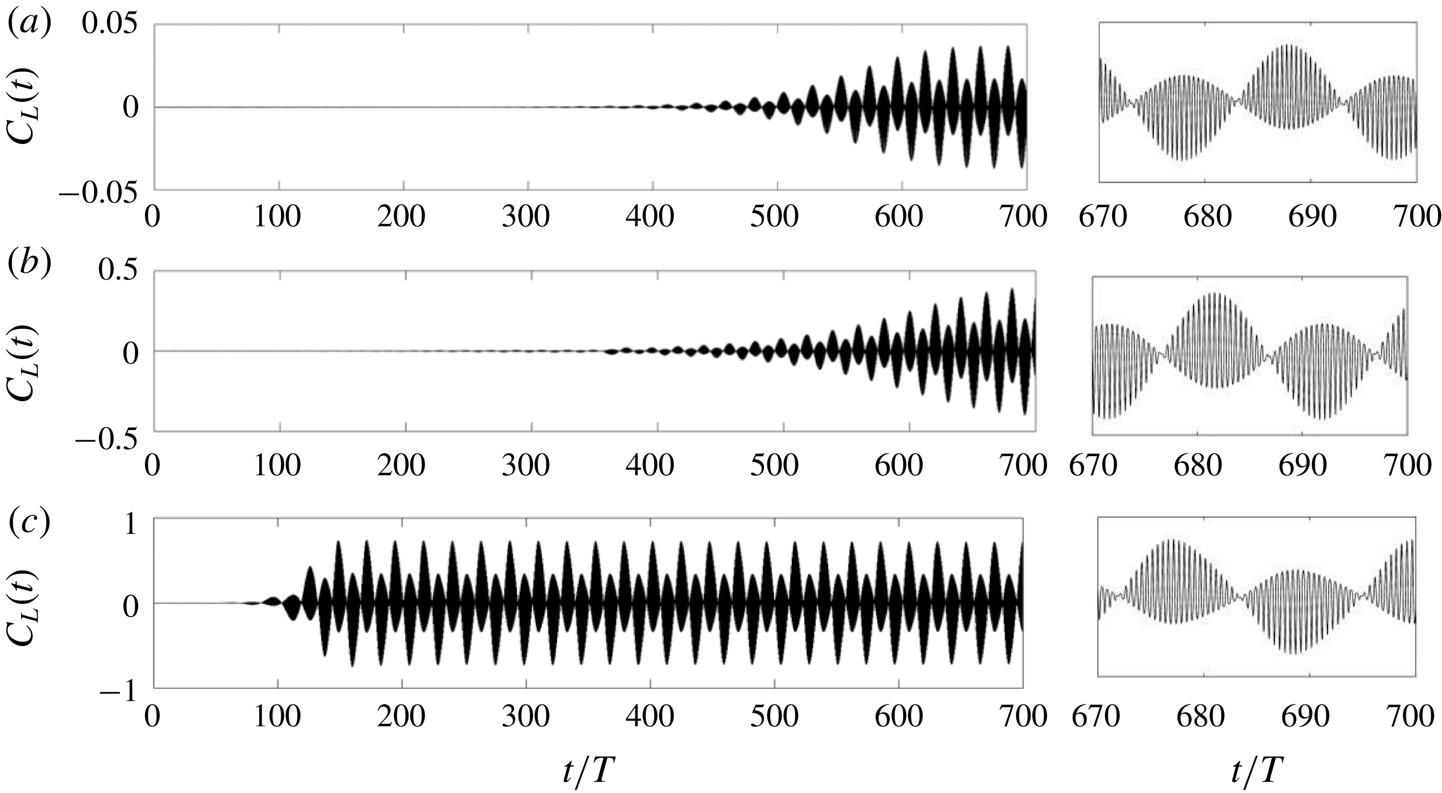
Transient transverse force coefficient and close-up view in the last 30 cycles at
 $KC=5$
and
 $\unicode[STIX]{x1D6FD}=32.4$
, 33 and 34 (from top to bottom). The corresponding frequencies for the secondary period are
 $f_{s}T=0.049$
, 0.044 and 0.041.

A series of 2-D DNS are then performed to quantify the 2-D nonlinear effect. The transient lift coefficient
 $C_{L}$
is plotted in figure 7. The appearance of a non-zero transverse force suggests the onset of flow instabilities (
 $K_{x}$
symmetry breaking and vortex shedding). Once the flow instability is initiated, the amplitude of
 $C_{L}$
increases with time and eventually reaches an equilibrium value due to the nonlinear effect. Due to the low growth rate of the instability near the critical point, it takes almost 400 cycles for the flow to reach an equilibrium state at
 $\unicode[STIX]{x1D6FD}=32.4$
and 350 cycles at
 $\unicode[STIX]{x1D6FD}=33$
. The number of cycles required for the development of an equilibrium state after the onset of instabilities decreases with increasing
 $\unicode[STIX]{x1D6FD}$
due to the increasing nonlinear effect (induced by the increasing strength of flow instabilities with
 $\unicode[STIX]{x1D6FD}$
). For example, an equilibrium state for
 $\unicode[STIX]{x1D6FD}=34$
is reached in approximately 150 cycles, which is significantly less than the 400 cycles at
 $\unicode[STIX]{x1D6FD}=32.4$
and 350 cycles at
 $\unicode[STIX]{x1D6FD}=33$
. The amplitude of the lift coefficient
 $C_{L}^{A}$
, defined as
 $[(C_{L})_{max}-(C_{L})_{min}]/2$
, also increases with
 $\unicode[STIX]{x1D6FD}$
(e.g.
 $0.040$
at
 $\unicode[STIX]{x1D6FD}=32.4$
, 0.382 at
 $\unicode[STIX]{x1D6FD}=33$
and 0.747 at
 $\unicode[STIX]{x1D6FD}=34$
) due to the increasing strength of flow instabilities with
 $\unicode[STIX]{x1D6FD}$
.
The Floquet analysis based on symmetric base flows becomes less convincing as
 $\unicode[STIX]{x1D6FD}$
increases beyond the critical symmetry breaking value (
 $\unicode[STIX]{x1D6FD}_{cr}$
) because it is not able to provide reliable information about the 3-D instability at further higher
 $\unicode[STIX]{x1D6FD}$
. Following Elston (Reference Elston2006), stability analysis based on a single 3-D instability mode is conducted for a range of
 $\unicode[STIX]{x1D6FD}$
beyond
 $\unicode[STIX]{x1D6FD}_{cr}$
, and the results are shown in figure 8. The single-mode stability analysis removes the enforcement of
 $K_{x}$
symmetry and introduces a single-mode 3-D instability with a wavelength of
 $L_{z}$
by setting
 $N_{z}=4$
. The single-mode analysis is much more computationally efficient than the full 3-D DNS, and it is able to provide realistic information about the evolution of 3-D instabilities with wavenumber. The results shown in figure 8 are similar to those shown in figure 7.18 of Elston (Reference Elston2006), who studied the instability at a fixed
 $\unicode[STIX]{x1D6FD}=40$
and
 $4.6\leqslant KC\leqslant 5.2$
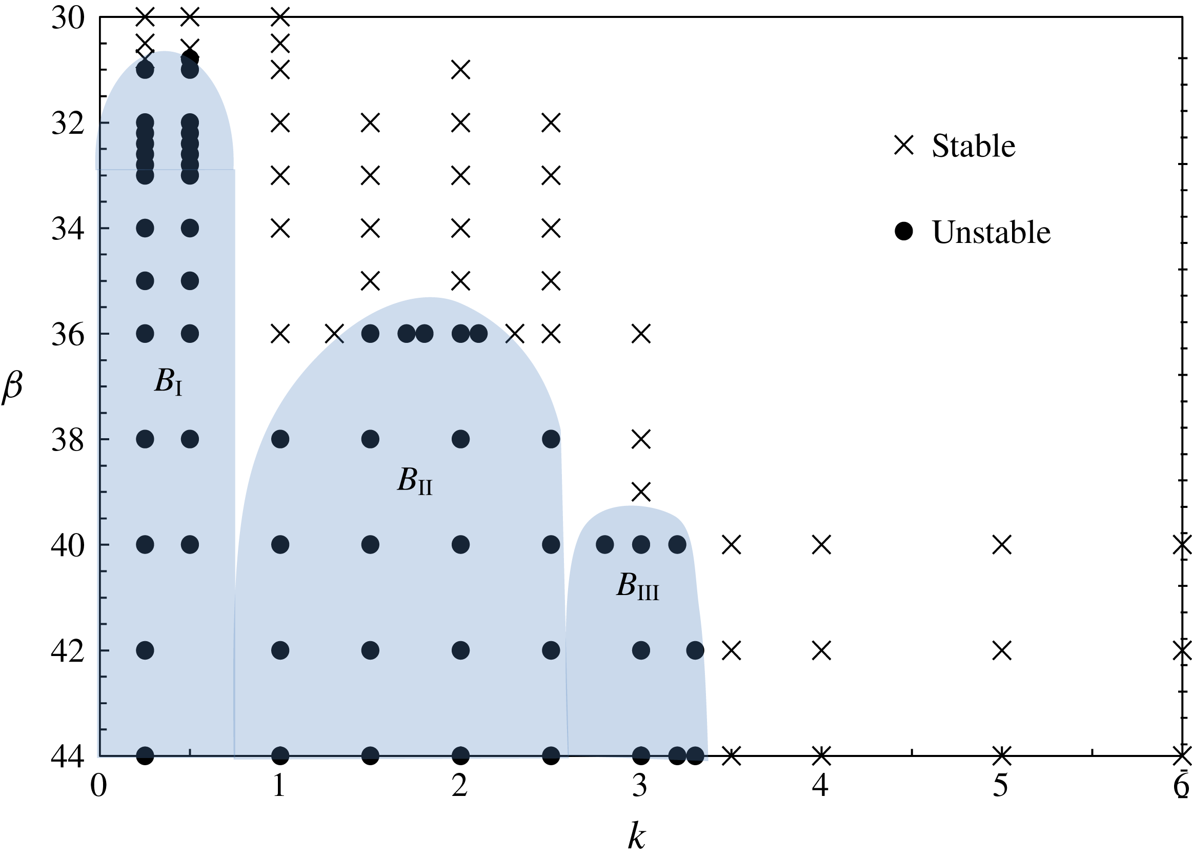
. Three bands
 $B_{\text{I}}$
,
 $B_{\text{II}}$
and
 $B_{\text{III}}$
of 3-D instabilities are identified, and the points for the onset of the instability of each band are indicated in figure 1(b):
Results of single-mode 3-D stability analysis at fixed
 $KC=5$
and
 $30\leqslant \unicode[STIX]{x1D6FD}\leqslant 44$
. The shaded regions indicate three bands of unstable 3-D instability.

(i) the band of instability
 $B_{\text{I}}$
emerges at approximately
$\unicode[STIX]{x1D6FD}_{cr}\approx 30.8$
and
$k\approx 0.5$
, which is lower than
$\unicode[STIX]{x1D6FD}_{cr}=32.0$
at
$k=0.375$
predicted by the Floquet analysis (figure 4), demonstrating the subcritical nature of the 3-D bifurcation,
(ii) the band
$B_{\text{II}}$
is centred at
$\unicode[STIX]{x1D6FD}\approx 35\sim 36$
and
$k\approx 1.75$
, which was attributed to the instability arising from regime-D-like structures in the flow by Elston et al. (Reference Elston, Blackburn and Sheridan2006),(iii) the band
$B_{\text{III}}$
is centred around
$\unicode[STIX]{x1D6FD}\approx 39\sim 40$
and
$k\approx 3$
, where the spanwise vortex pattern has been categorised into regime E.


These results agree well with the experimental results for both the lower and upper limits of
 $\unicode[STIX]{x1D6FD}$
that bound the regime C, as shown in figure 1.
The above analysis shows that the lower bound
 $\unicode[STIX]{x1D6FD}_{cr}$
for mode C is decreased from
 $\unicode[STIX]{x1D6FD}_{cr}=32.0$
to
 $\unicode[STIX]{x1D6FD}\approx 30.8$
by the single-mode 3-D instability analysis that is seeded with low-wavenumber disturbances. This substantially narrows the gap between the
 $\unicode[STIX]{x1D6FD}_{cr}$
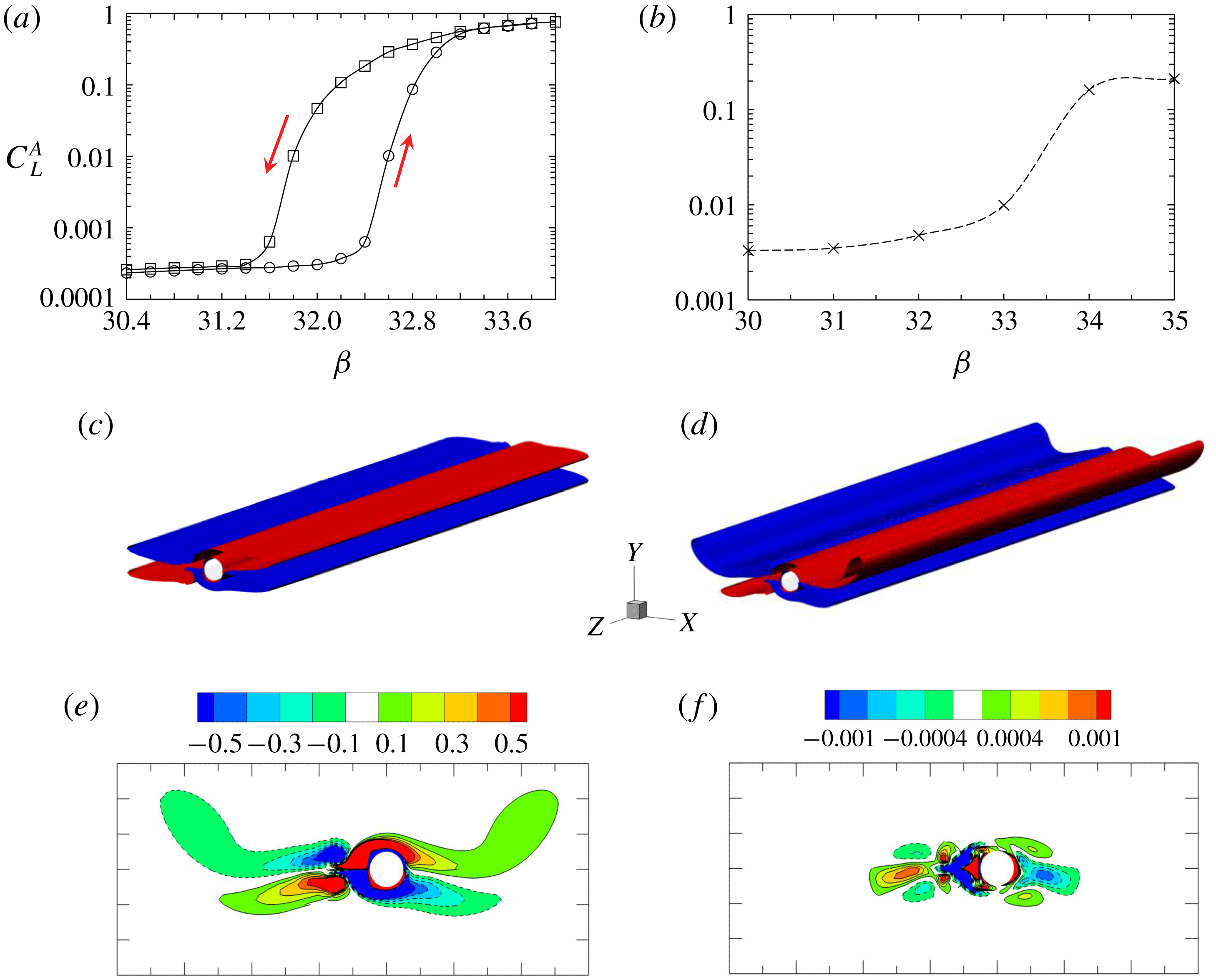
values obtained by the physical experiments and the stability analysis. The subcritical nature of the mode C instabilities is attributed to the disparity between the predicted (2-D Floquet analysis) and observed (experimental and numerical) lower bounds of
 $\unicode[STIX]{x1D6FD}_{cr}$
for regime C. This point will be further elaborated in § 3.4.
3.2 Influence of the spanwise length
In 3-D DNS, the spanwise length (
 $L_{z}$
) of the computational domain is an important parameter that potentially affects the simulation results. The Floquet analysis conducted in this study shows that the 3-D instability occurs first at low wavenumbers (lower branch). This finding suggests that a large spanwise length is required to resolve the 3-D flow. To determine an appropriate
 $L_{z}$
, the influence of the spanwise length of the computational domain is investigated.
A series of 3-D simulations are conducted at
 $(KC,\unicode[STIX]{x1D6FD})=(5,34)$
with a range of spanwise lengths of
 $L_{z}=\unicode[STIX]{x03C0}$
,
 $2\unicode[STIX]{x03C0}$
,
 $4\unicode[STIX]{x03C0}$
,
 $8\unicode[STIX]{x03C0}$
and
 $16\unicode[STIX]{x03C0}$
. The order of Fourier mode
 $m$
is converted to wavenumber as
 $k=2\unicode[STIX]{x03C0}m/L_{z}$
. Thus, the wavenumber resolved in the simulation ranges from
 $k_{min}=2\unicode[STIX]{x03C0}/L_{z}$
to
 $k_{max}=2\unicode[STIX]{x03C0}(N/2-1)/L_{z}=(N-2)\unicode[STIX]{x03C0}/L_{z}$
with an interval of
 $\unicode[STIX]{x0394}k=2\unicode[STIX]{x03C0}/L_{z}$
, where
 $N$
denotes the spanwise resolution (see figure 2). Since 3-D instabilities for flows in regime C occur within the three bands
 $B_{\text{I}{-}\text{III}}$
of relatively low wavenumbers
 $k<3.5$
for
 $\unicode[STIX]{x1D6FD}<44$
(figure 8), a spanwise resolution of
 $N=64$
(
 $m_{max}=31$
) is deemed to be sufficient to resolve all 3-D instabilities of the flow in regime C, which has been confirmed by the convergence test presented in the Appendix. Therefore,
 $N$
is fixed at 64 in the five simulation cases considered, with different
 $L_{z}$
values for simplicity, and the sequence of complex Fourier modes is up to 32.
For each case, the simulated time has been extended to at least 300 cycles to ensure fully developed instabilities. The sectional lift force
 $C_{L}(z,t)$
on 64 equi-spaced slices and the modal energy
 $E_{m}(t)$
with
 $m$
ranging from 0 to 31 are sampled at a time interval of
 $\unicode[STIX]{x0394}t/T=1/250$
. The modal energy
 $E_{m}(t)$
is estimated by
 $$\begin{eqnarray}\displaystyle & \displaystyle E={\displaystyle \frac{1}{L_{z}}}\int _{0}^{L_{z}}\int _{\unicode[STIX]{x1D6FA}}\left\Vert \hat{\boldsymbol{u}}_{m}^{c}(x,y,t)\text{cos}\left({\displaystyle \frac{2m\unicode[STIX]{x03C0}z}{L_{z}}}\right)+\hat{\boldsymbol{u}}_{m}^{s}(x,y,t)\text{sin}\left({\displaystyle \frac{2m\unicode[STIX]{x03C0}z}{L_{z}}}\right)\right\Vert ^{2}\,\text{d}\unicode[STIX]{x1D6FA}\,\text{d}z.\quad & \displaystyle\end{eqnarray}$$
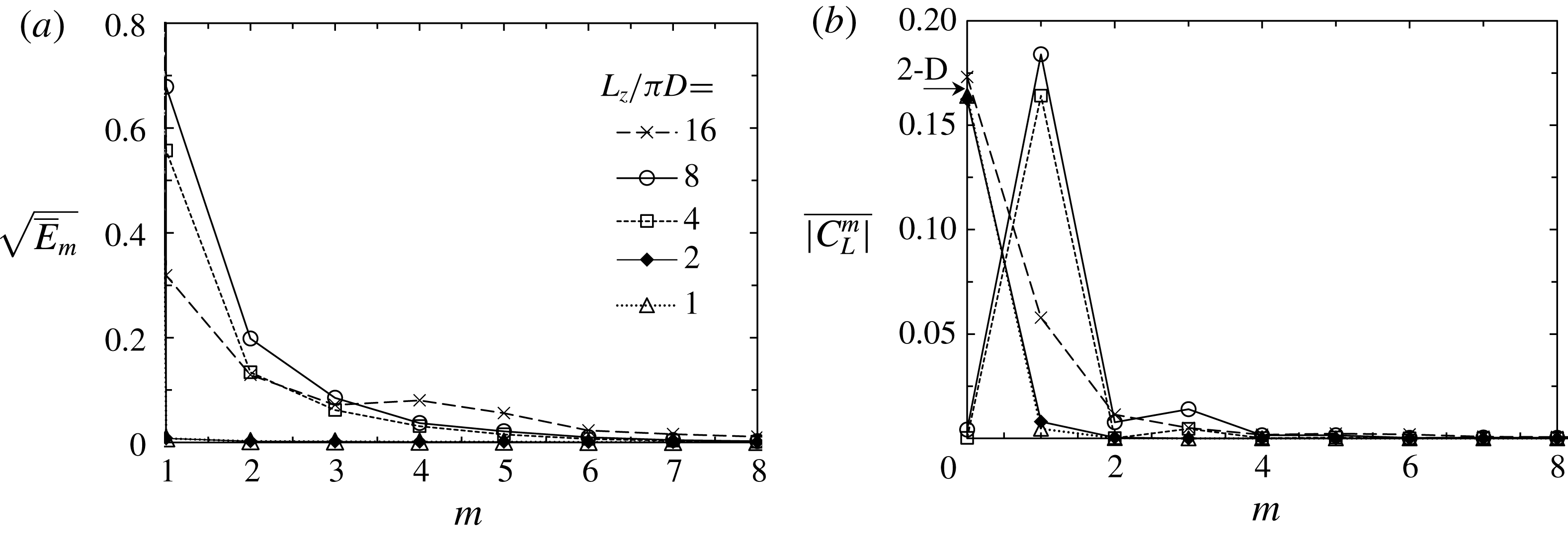
The three-dimensionality of the flow is examined by the mean 3-D modal kinetic energy
 $\overline{E}_{m}$
based on the results obtained in the last 100 cycles of the simulation (figure 9
a), and the spectrum of the mean magnitude of the lift coefficient
 $\overline{|C_{L,m}|}$
at each Fourier mode (figure 9
b), where
 $C_{L,m}(t)$
is obtained through a spatial Fourier transform of
 $C_{L}(z,t)$
.
(a) Mean 3-D modal kinetic energy and (b) the spectrum of the mean absolute value of the lift coefficient of different Fourier modes at
 $(KC,\unicode[STIX]{x1D6FD})=(5,34)$
(where the 2-D result is given by an arrow on the vertical axis). The results are averaged for the last 100 cycles, which is up to
 $t/T\sim 300$
for
 $L_{z}/\unicode[STIX]{x03C0}=1$
, 2, 4 and 8 (and the 2-D case) and up to
 $t/T=1000$
for
 $L_{z}/\unicode[STIX]{x03C0}=16$
.

For
 $L_{z}=\unicode[STIX]{x03C0}$
or
 $2\unicode[STIX]{x03C0}$
, the flow is almost two-dimensional because
 $E_{m}$
is trivial at non-zero modes. This result is expected because the 3-D instability at
 $k_{min}=2$
or 1 is stable at
 $\unicode[STIX]{x1D6FD}=34$
according to the Floquet analysis results shown in figure 4 and the single-mode analysis results shown in figure 8. However, the 3-D energy emerges in the simulations with
 $L_{z}=4\unicode[STIX]{x03C0}$
and
 $8\unicode[STIX]{x03C0}$
, and the leading 3-D instabilities of both are observed at
 $m=1$
, corresponding to
 $k_{min}=2\unicode[STIX]{x03C0}/4\unicode[STIX]{x03C0}=0.5$
for
 $L_{z}=4\unicode[STIX]{x03C0}$
and
 $k_{min}=2\unicode[STIX]{x03C0}/8\unicode[STIX]{x03C0}=0.25$
for
 $L_{z}=8\unicode[STIX]{x03C0}$
. Figure 9(b) shows that the fully developed
 $\overline{|C_{L,m=0}|}$
is similar to the 2-D result and the absence of 3-D instabilities for
 $L_{z}=\unicode[STIX]{x03C0}$
and
 $2\unicode[STIX]{x03C0}$
. The magnitudes of
 $\overline{|C_{L,m=0}|}$
are much smaller than those of
 $\overline{|C_{L,m=1}|}$
for
 $L_{z}=4\unicode[STIX]{x03C0}$
and
 $8\unicode[STIX]{x03C0}$
, which indicates that the 2-D instability has been suppressed by the onset of the 3-D instability at
 $m=1$
. The results shown in figure 9 indicate that the spanwise convergence has not been achieved for up to
 $L_{z}=16\unicode[STIX]{x03C0}$
.
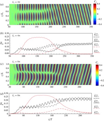
The temporal evolution and convergence of the 3-D instabilities for
 $L_{z}=4\unicode[STIX]{x03C0}$
and
 $8\unicode[STIX]{x03C0}$
are further investigated in figure 10 by plotting the
 $C_{L}(z,t)$
contour in the plane of
 $(z/L_{z},t)$
and tracking the kinetic energy of the cosine part
 $E_{m}^{cos}$
and sine part
 $E_{m}^{sin}$
of the Fourier modes at
 $m=1$
and 2. The amplitudes of
 $E_{m=1}^{cos}$
and
 $E_{m=1}^{sin}$
are almost identical for
 $t/T<120$
with
 $L_{z}=4\unicode[STIX]{x03C0}$
(figure 10
b) and
 $t/T<80$
with
 $Lz=8\unicode[STIX]{x03C0}$
(figure 10
d). Then, the deviations between them become clear until approximately
 $t/T=250$
for
 $L_{z}=4\unicode[STIX]{x03C0}$
and
 $t/T=230$
for
 $L_{z}=8\unicode[STIX]{x03C0}$
. They then both reach the equilibrium state with a fixed phase difference of approximately
 $\unicode[STIX]{x03C0}/2$
. In contrast,
 $E_{m=2}^{sin}$
transiently increases to a higher level than that at
 $m=1$
and remains stable at approximately
 $t/T=120\sim 180$
for
 $L_{z}=4\unicode[STIX]{x03C0}$
and
 $t/T=110\sim 170$
for
 $L_{z}=8\unicode[STIX]{x03C0}$
before it subsequently diminishes.
 $E_{m=2}^{cos}$
reaches a peak at approximately
 $t/T=220$
for
 $L_{z}=4\unicode[STIX]{x03C0}$
and
 $t/T=210$
for
 $L_{z}=8\unicode[STIX]{x03C0}$
before gradually diminishing soon after.
(a,c) The contour of sectional lift coefficient and (b,d) the kinetic energy of the cosine part
 $\hat{\boldsymbol{u}}_{m}^{c}$
and sine part
 $\hat{\boldsymbol{u}}_{m}^{s}$
of the primary and secondary Fourier modes at
 $(KC,\unicode[STIX]{x1D6FD})=(5,34)$
. Note that the kinetic energy is sampled discontinuously from the flow field at
 $t/T=1,2,\ldots ,n$
.

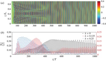
(a) The contour of the sectional lift coefficient and (b) the corresponding cycle-to-cycle-averaged modal amplitude
 $\overline{|C_{L}^{k}|}=[\int _{(n-1)T}^{nT}|C_{L}^{k}|\,\text{d}t]/T$
at wavenumbers
 $k=0$
, 0.125 and 0.25 at
 $(KC,\unicode[STIX]{x1D6FD})=(5,34)$
for
 $L_{z}=16\unicode[STIX]{x03C0}$
, where the 2-D component (
 $k=0$
) corresponds to the
 $y$
-axis on the left and the 3-D component (
 $k=0.125$
and 0.25) corresponds to the
 $y$
-axis on the right side.

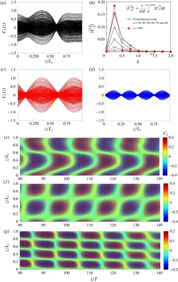
Figure 10(a) shows that the sectional
 $C_{L}(z)$
for
 $L_{z}=4\unicode[STIX]{x03C0}$
varies similarly to a standing wave with a periodically changing amplitude and two fixed nodes at
 $z/L_{z}\approx 0.1$
and 0.6 for
 $t/T<150$
. Then, the nodes transitionally move towards the high
 $z/L_{z}$
value direction and become less distinctive between
 $t/T=150$
and 200. Finally, the sectional
 $C_{L}(z)$
behaves similar to a stable travelling wave in a direction from high to low
 $z/L_{z}$
values. Although the sectional
 $C_{L}(z)$
for
 $L_{z}=8\unicode[STIX]{x03C0}$
also forms into a travelling wave, several distinct differences between figures 10(a) and 10(c) are observed: (i) the latter one appears similar to a spatial combination of a travelling wave and a standing wave at the initial stage; (ii) there is no node at
 $z/L_{z}\approx 0.1$
, and the one at
 $z/L_{z}\approx 0.6$
is less distinctive than the former one; and (iii) the travelling wave propagates in the direction from low to high
 $z/L_{z}$
values, which is opposite to that observed in the case with
 $L_{z}=4\unicode[STIX]{x03C0}$
.
The simulation time with
 $L_{z}=16\unicode[STIX]{x03C0}$
has been extended significantly (beyond 1000) to achieve an equilibrium state. This effort did not achieve a satisfactory outcome, as shown in figure 11, where considerable variations in the sectional
 $C_{L}(z)$
are observed beyond
 $t/T>1000$
. The results obtained with
 $L_{z}=16\unicode[STIX]{x03C0}$
are somewhat surprising because (i) both 2-D and leading 3-D instabilities show clear variations with time and have not reached equilibrium states up to
 $t/T=1000$
, and (ii) the 2-D instability is neither dominating over the 3-D instability, similar to the cases for
 $L_{z}=\unicode[STIX]{x03C0}$
or
 $2\unicode[STIX]{x03C0}$
, nor diminishing as the cases for
 $L_{z}=4\unicode[STIX]{x03C0}$
or
 $8\unicode[STIX]{x03C0}$
(figure 9). Given the high computational cost and no indication of convergence, the simulation was discontinued shortly after
 $t/T>1000$
. The contour of sectional
 $C_{L}(z)$
is similar to that for
 $L_{z}=8\unicode[STIX]{x03C0}$
, and the leading 3-D instability is larger than the 2-D instability according to the modal sectional
 $C_{L}(z)$
over the first 200 cycles. However, it does not evolve into a travelling mode afterwards. Rather, the 2-D instability is dominating over the 3-D instability, leading to a relatively uniform contour of
 $C_{L}(z)$
along the axis. Although the 3-D components for
 $k\geqslant 0.25$
all diminish after
 $t\approx 500$
, the leading 3-D instability at
 $k=0.125$
increases again, and the modulation of the 2-D component by the secondary frequency continues to grow.
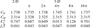
Comparison of drag (
 $C_{D}$
) and inertia (
 $C_{M}$
) force coefficients, the amplitude of the lift coefficient
 $C_{L}^{A}$
and normalised secondary frequency
 $f_{S}T$
among 2-D simulation and 3-D cases with different wavelengths at
 $(KC,\unicode[STIX]{x1D6FD})=(5,34)$
.
 $C_{D}$
and
 $C_{M}$
are determined by the Morison equation
 $F_{x}=1/2\unicode[STIX]{x1D70C}DC_{D}|U(t)|U(t)+1/4\unicode[STIX]{x1D70C}D^{2}C_{M}\,\text{d}U(t)/\text{d}t$
, where
 $\unicode[STIX]{x1D70C}$
is the density of fluid. The secondary frequency
 $f_{s}T$
is obtained from a fast Fourier transform (FFT). The results are determined from the data during
 $t/T=200\sim 300$
for
 $L_{z}/\unicode[STIX]{x03C0}=1$
, 2, 4 and 8, and are determined during
 $t/T=900\sim 1000$
for
 $L_{z}/\unicode[STIX]{x03C0}=16$
.

The influence of
 $L_{z}$
on hydrodynamic forces is quantified in table 1 by comparing the drag (
 $C_{D}$
) and inertia (
 $C_{M}$
) coefficients, the amplitude (
 $C_{L}^{A}$
) and the frequency (
 $f_{S}T$
) of
 $C_{L}$
calculated from 2-D and 3-D simulations at
 $(KC,\unicode[STIX]{x1D6FD})=(5,34)$
. Only slight differences are found for the inline force coefficients between the 2-D and 3-D simulation results. This result agrees well with the finding by Nehari et al. (Reference Nehari, Armenio and Ballio2004) that the inline force is only weakly affected by the three-dimensionality. The
 $C_{L}^{A}$
, however, shows a clear dependence on
 $L_{z}$
. The largest
 $C_{L}^{A}$
of 0.747 is obtained by the 2-D simulation. As
 $L_{z}$
increases from
 $\unicode[STIX]{x03C0}$
to
 $16\unicode[STIX]{x03C0}$
,
 $C_{L}^{A}$
initially decreases and drops to approximately 1 % of that predicted by the 2-D simulation with
 $L_{z}=4\unicode[STIX]{x03C0}$
; then,
 $C_{L}^{A}$
increases again with
 $L_{z}$
and reaches approximately 0.7 at
 $L_{z}=16\unicode[STIX]{x03C0}$
. In general,
 $C_{L}^{A}$
is significantly affected by the 3-D flow patterns, which is discussed below in detail based mainly on the results obtained with
 $L_{z}=4\unicode[STIX]{x03C0}$
and
 $8\unicode[STIX]{x03C0}$
(only briefly based on the results obtained with
 $L_{z}=16\unicode[STIX]{x03C0}$
).
The difference between the results of
 $L_{z}=4\unicode[STIX]{x03C0}$
and
 $8\unicode[STIX]{x03C0}$
is attributable to the low-wavenumber instability introduced as
 $L_{z}$
is increased from
 $4\unicode[STIX]{x03C0}$
to
 $8\unicode[STIX]{x03C0}$
, as evidenced by the results shown in figures 4 and 8. Since the wave resolution (
 $1/\unicode[STIX]{x0394}k=L_{z}/2\unicode[STIX]{x03C0}$
) increases with
 $L_{z}$
, new perturbations with lower wavenumbers than those in the simulation with
 $L_{z}=4\unicode[STIX]{x03C0}$
emerge and interact with other perturbations nonlinearly in the simulation with
 $L_{z}=8\unicode[STIX]{x03C0}$
. As the simulation progresses, all 3-D instabilities coalesce at the leading wavenumber, thus forming a pattern similar to those shown in figure 10(a,c). As illustrated in figure 9, temporal and spatial convergences of the leading wavenumber were not achieved by a further simulation with
 $L_{z}=16\unicode[STIX]{x03C0}$
. The leading 3-D instability is no longer dominated by the primary Fourier mode (
 $m=1$
) but rather by a Fourier mode with a wavenumber close to the wavenumber (
 $k=0.203$
at
 $KC=5$
and
 $\unicode[STIX]{x1D6FD}=34$
, as shown in figure 4
a) at which the maximum Floquet multiplier occurs. Since new perturbations with smaller wavenumbers will inevitably be introduced with increasing
 $L_{z}$
, it is almost practically impossible to achieve a spatial convergence for 3-D simulations with available computational resources. Despite this situation, the predicted 3-D vortex patterns are nonetheless similar to those observed in the physical experiments. The flow characteristics will be investigated based largely on the results obtained with
 $L_{z}=4\unicode[STIX]{x03C0}$
and
 $8\unicode[STIX]{x03C0}$
in the following discussions, with an expectation that they reflect the characteristics of the flow. The observed results shown in this section are explained in detail in § 3.3 based on the results of the stability analysis reported in § 3.1.
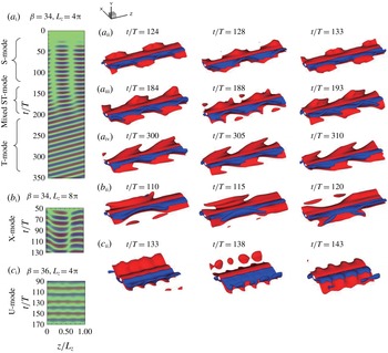
Overview of the five typical vortex patterns/modes shown by the contour of the sectional lift coefficient with colour map
 $-0.4\leqslant C_{L}\leqslant 0.4$
for (
 $a_{\text{i}},b_{\text{i}}$
) and
 $-0.8\leqslant C_{L}\leqslant 0.8$
for (
 $c_{\text{i}}$
), and instantaneous iso-surfaces of
 $\unicode[STIX]{x1D714}_{z}=\pm 0.15$
are shown. Two spanwise repetitions are plotted for (
 $a_{\text{ii}{-}\text{iv}}$
).

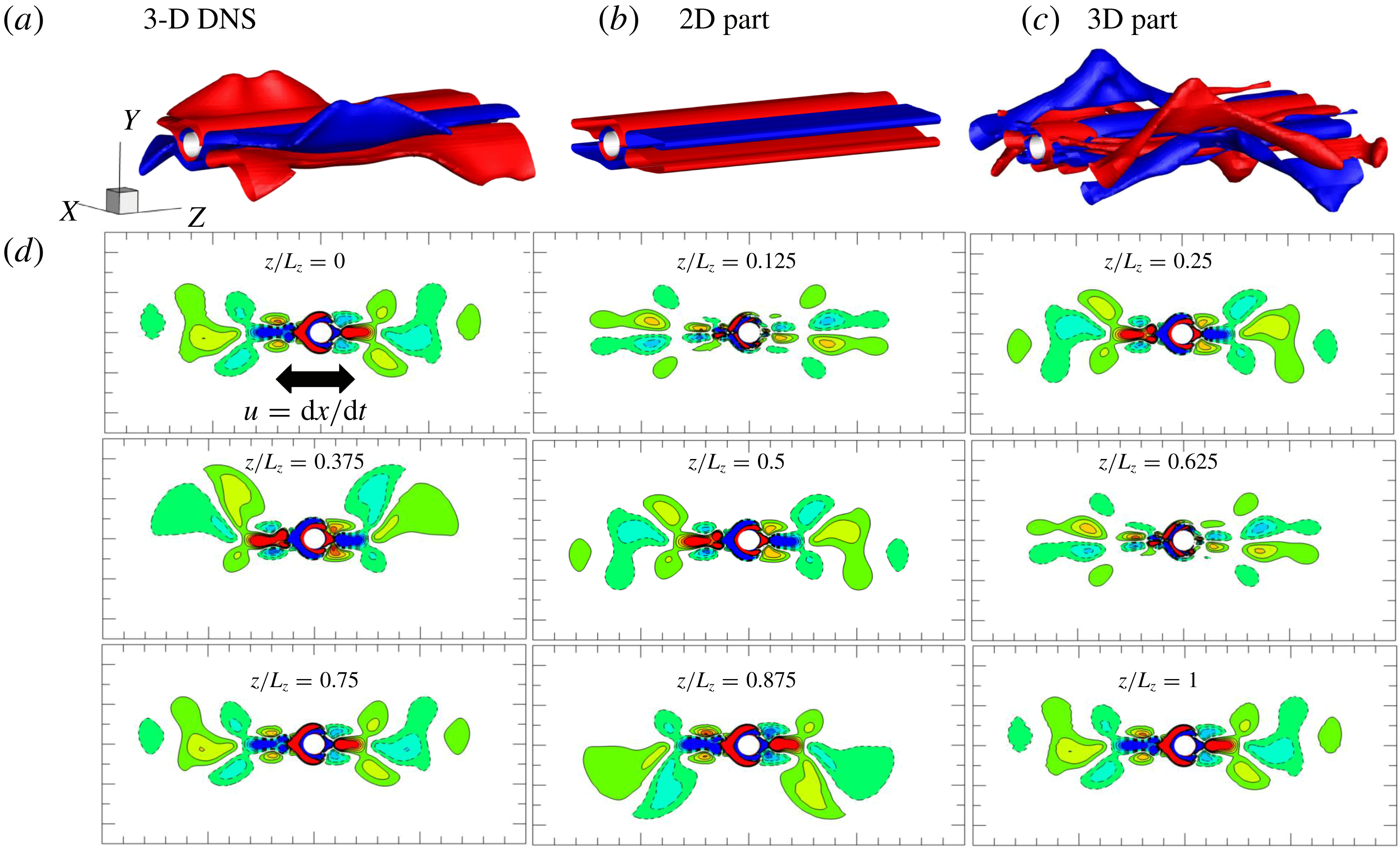
The S-mode for the case shown in figure 12(a) at
 $t/T=124.15$
when the amplitude of the secondary lift force reaches a local peak. (a–c) The vorticity iso-surface of
 $\unicode[STIX]{x1D714}_{z}=\pm 0.15$
: (a) full DNS, (b) 2-D component of DNS and (c) 3D component of DNS. (d) Cross-sectional views of vorticity contour of
 $-0.25\leqslant \unicode[STIX]{x1D714}_{z}\leqslant 0.25$
.

3.3 Three-dimensional flow pattern
The full 3-D DNS are mainly performed at a fixed
 $KC=5$
for
 $\unicode[STIX]{x1D6FD}$
ranging from 32 to 38 with an interval of
 $\unicode[STIX]{x0394}\unicode[STIX]{x1D6FD}=2$
. A few cases at
 $\unicode[STIX]{x1D6FD}=40$
are examined for the purpose of validation against Elston et al. (Reference Elston, Blackburn and Sheridan2006) and at
 $KC=4.4$
for validation against Tatsuno & Bearman (Reference Tatsuno and Bearman1990). Herein, only the results at
 $\unicode[STIX]{x1D6FD}=34$
and 36 are presented due to the similarities shared by the other cases. As shown in figure 12, five typical flow patterns/modes are observed, including
(i) the S-mode featured by sinusoidal axial variation in sectional vorticity in a form similar to a standing wave, with S representing the standing;
(ii) the T-mode featured by a travelling wave along the span of the cylinder in the form of a V-type vortex pattern, with T representing the travelling;
(iii) the mixed ST-mode characterised by a mixture of the standing–travelling wave and saddle points in the force distribution;
(iv) the X-mode characterised by X-type vortex patterns; and
(v) the U-mode characterised by a unidirectional oblique angle along the axis of the cylinder.
The flow structures and axial modulation of
 $C_{L}(z)$
in each of the modes identified above are described below.
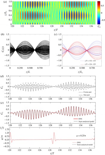
Investigation of sectional lift coefficient in the S-mode, following the same case as figure 12(a). (a) A local contour of sectional lift coefficient (
 $C_{L}(t,z)$
). (b) The transient sectional
 $C_{L}(z)$
in the plane of
 $z/L_{z}-C_{L}$
. (c) The transient sectional
 $C_{L}(z)$
from
 $t/T$
= 124 to 125 and 132 to 133 with an interval
 $\unicode[STIX]{x0394}t/T=0.04$
. (d) The transient spatial amplitude of the lift coefficient contributed by the cosine part and sine part. (e) The overall transient spatial amplitude of the lift coefficients at
 $m=1$
, extracted from DNS and predicted using the model. (f) The transient spanwise phase angle
 $\unicode[STIX]{x1D711}$
of sectional
 $C_{L}(z)$
at
 $m=1$
, extracted from DNS and predicted using the model.

3.3.1 S-mode
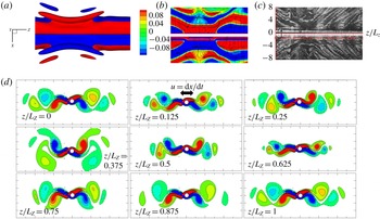
Figure 13 illustrates a typical S-mode vortex structure at
 $(KC,\unicode[STIX]{x1D6FD})=(5,34)$
with
 $L_{z}=4\unicode[STIX]{x03C0}$
by decoupling the 2-D and 3-D components in (a–c) and cross-sectional flow field in (d). According to (2.4), the 2-D component extracted from the wave space of the flow field at
 $m=0$
(figure 13
b) is equivalent to the spanwise-averaged flow field shown in figure 13(a). The 2-D component (
 $m=0$
) of the 3-D simulation still generally possesses
 $K_{x}$
symmetry, whereas that from the 2-D simulation at the same (
 $KC$
,
 $\unicode[STIX]{x1D6FD}$
) shows clear asymmetry, which is due to the suppression of the 2-D instability by the onset of 3-D instability in the 3-D simulation as discussed in § 3.2. The remaining 3-D component (figure 13
c) is obtained by subtracting the 2-D component from the overall flow field. The S-mode structure is observed clearly in figure 13(c). The sectional vorticity contours are almost symmetric about the
 $x$
-axis at
 $z/L_{z}=0.125$
and 0.625, whereas the most asymmetric patterns are observed at
 $z/L_{z}=0.375$
and 0.875. The cross-sectional flow in figure 13(c) possesses
 $z$
translation–reflection symmetry, which is defined by
 $$\begin{eqnarray}\displaystyle & \displaystyle Z_{x}:\unicode[STIX]{x1D714}_{z}(x,y,z,t)=-\unicode[STIX]{x1D714}_{z}(x,-y,z+L_{z}/2,t). & \displaystyle\end{eqnarray}$$
The dynamic loads, particularly their spanwise variations, are found to be closely associated with the three-dimensionality of the vorticity field of the flow. A more elaborate view of the
 $C_{L}(z)$
contour extracted from figure 10(a) is replotted by using the same data in the (
 $z/L_{z}$
,
 $C_{L}$
)-plane with a time interval of
 $\unicode[STIX]{x0394}t/T=0.04$
, as shown in figure 14(a). The standing-wave pattern of
 $C_{L}(z)$
in the
 $z$
-direction, with two fixed nodes at approximately
 $z/L_{z}=0.125$
and 0.625 and two fixed peak points at
 $z/L_{z}=0.375$
and 0.875, is clearly observed in figure 14(a) and further confirmed in figure 14(b). The node and peak positions correspond to the locations of the most symmetric and most asymmetric vortex patterns, respectively (figure 13
d). Furthermore, the distribution of sectional lift force at any instant is very similar to a sinusoidal function, which can be expressed in the form
 $$\begin{eqnarray}\displaystyle & \displaystyle C_{L}(t,z)=C_{L}^{A}(t)\text{cos}\left({\displaystyle \frac{2\unicode[STIX]{x03C0}z}{L_{z}}}+\unicode[STIX]{x1D711}\right), & \displaystyle\end{eqnarray}$$
where
 $C_{L}^{A}(t)$
is a time-dependent function varying with the phases of streamwise oscillation
 $\unicode[STIX]{x1D70F}=t/T-n$
and secondary oscillation
 $\unicode[STIX]{x1D6FC}=2\unicode[STIX]{x03C0}f_{s}t+\unicode[STIX]{x1D6FC}_{0}$
. Based on (3.9), the positions of the node and peak points are determined as
 $$\begin{eqnarray}\displaystyle & \displaystyle \left({\displaystyle \frac{z}{L_{z}}}\right)_{node}={\displaystyle \frac{\unicode[STIX]{x03C0}-2\unicode[STIX]{x1D711}}{4\unicode[STIX]{x03C0}}}\text{ or }{\displaystyle \frac{3\unicode[STIX]{x03C0}-2\unicode[STIX]{x1D711}}{4\unicode[STIX]{x03C0}}}, & \displaystyle\end{eqnarray}$$
 $$\begin{eqnarray}\displaystyle & \displaystyle \left({\displaystyle \frac{z}{L_{z}}}\right)_{peak}={\displaystyle \frac{\unicode[STIX]{x03C0}-\unicode[STIX]{x1D711}}{2\unicode[STIX]{x03C0}}}\text{ or }{\displaystyle \frac{2\unicode[STIX]{x03C0}-\unicode[STIX]{x1D711}}{2\unicode[STIX]{x03C0}}}, & \displaystyle\end{eqnarray}$$
with a spanwise phase angle
 $\unicode[STIX]{x1D711}$
of
 $0.25\unicode[STIX]{x03C0}$
(figure 14
c).
To quantify the modal component of the spanwise variation in the transverse force, a spatial Fourier transform is performed on the sectional transverse force at every sampled instant. The results show that the mean magnitude peaks at
 $m=1$
, whereas the magnitudes of other Fourier modes are trivial. Thus, the spanwise variation in dynamic loads is mainly modulated by the Fourier mode at
 $m=1$
, which can be decoupled in the following form:
 $$\begin{eqnarray}\displaystyle & \displaystyle C_{L}(t,z)=C_{L}^{c}(t)\text{cos}(k\unicode[STIX]{x03C0}z)+C_{L}^{s}(t)\text{sin}(k\unicode[STIX]{x03C0}z), & \displaystyle\end{eqnarray}$$
where
 $C_{L}^{c}(t)$
and
 $C_{L}^{s}(t)$
are the cosine and sine parts of the Fourier mode. The decoupled results shown in figure 13(d) reveal that
 $C_{L}^{c}(t)$
and
 $C_{L}^{s}(t)$
are approximately the same in amplitude and of the opposite signs. Furthermore, (3.12) can be simplified as
 $$\begin{eqnarray}\displaystyle & \displaystyle C_{L}(t,z)=(C_{L}^{A})^{\prime }\text{sin}[k\unicode[STIX]{x03C0}z+\unicode[STIX]{x1D719}(t)]=C_{L}^{A}\text{cos}[k\unicode[STIX]{x03C0}z+\unicode[STIX]{x03C0}/2+\unicode[STIX]{x1D719}(t)], & \displaystyle\end{eqnarray}$$
with
 $(C_{L}^{A})^{\prime }=-C_{L}^{A}$
. The spatial phase angle
 $\unicode[STIX]{x1D719}$
is given by
 $$\begin{eqnarray}\displaystyle & \displaystyle \text{tan}\unicode[STIX]{x1D719}(t)={\displaystyle \frac{C_{L}^{c}(t)}{C_{L}^{s}(t)}}. & \displaystyle\end{eqnarray}$$
Because
 $C_{L}^{c}$
and
 $C_{L}^{s}$
are opposite in sign, the time-dependent coefficient
 $C_{L}^{A}(t)$
can be written as
 $$\begin{eqnarray}\displaystyle & \displaystyle C_{L}^{A}(t)=\sqrt{2}C_{L}^{c}(t), & \displaystyle\end{eqnarray}$$
with an invariable phase angle of
 $$\begin{eqnarray}\displaystyle & \displaystyle \unicode[STIX]{x1D711}=\unicode[STIX]{x03C0}/2+\unicode[STIX]{x1D719}=\unicode[STIX]{x03C0}/4. & \displaystyle\end{eqnarray}$$
The predicted results agree well with the results extracted from the DNS, which are plotted in figure 14(e,f). The large oscillations of the predicted phase angle shown in figure 14(f) are due to numerical errors (can easily be removed), which occur at the phase where
 $C_{L}^{s}$
is close to zero (see (3.14)). By substituting (3.16) into (3.10)–(3.11), the occurrence of the standing wave with two nodes at
 $z/L_{z}=0.125$
and 0.625 and two peaks at
 $z/L_{z}=0.375$
and 0.875 can be explained.
The instantaneous vorticity contour (
 $-0.25\leqslant \unicode[STIX]{x1D714}_{z}\leqslant 0.25$
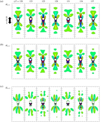
) of Fourier mode components, extracted from the wave space of the same case as figure 12(a) by Fourier decomposition for flow in the S-mode.

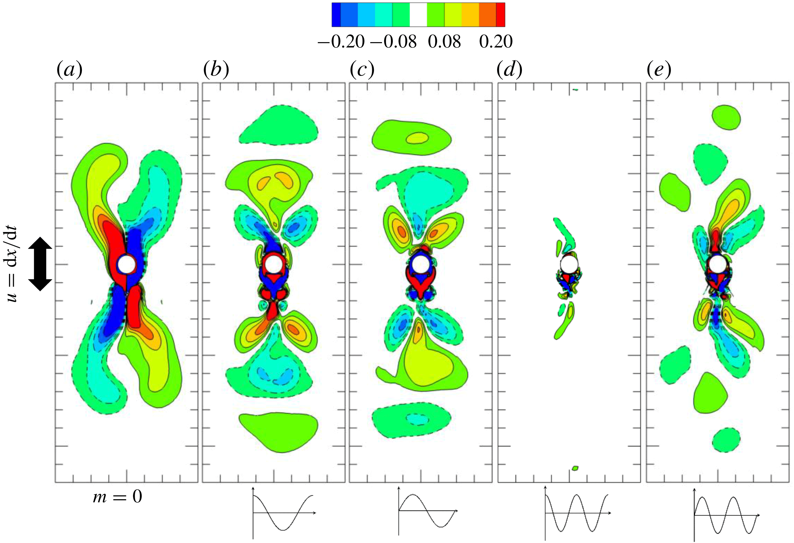
The S-mode is further demonstrated by visualising the Fourier mode components of
 $m=1$
and the sine part of
 $m=2$
in figure 15. The cosine part of
 $m=2$
is not shown here because it is trivial for the S-mode (figure 10
b). According to the Floquet analysis where
 $k=2\unicode[STIX]{x03C0}m/L_{z}$
, the only unstable Fourier mode that can be resolved with
 $L_{z}=4\unicode[STIX]{x03C0}$
is
 $m=1$
(
 $k=0.5$
). Therefore, the vorticity contours of the Fourier modes at
 $m=1$
are very similar to the eigenmodes shown in figure 5 and of an inverse
 $K_{x}$
symmetry. The large 3-D kinetic energy observed at
 $m=2$
(
 $k=0.25$
) is attributable to the nonlinear effect because the vorticity contours in figure 15(c) are clearly different from the counterpart obtained from the Floquet stability analysis by solving the linearised N–S equations (figure 5
c), particularly in terms of the symmetry status. Since the flow is generally of
 $K_{x}$
symmetry, it does not induce a lift force around the cylinder, even though its 3-D kinetic energy is the largest during
 $t/T=90$
to 200, as shown in figure 10.
3.3.2 T-mode
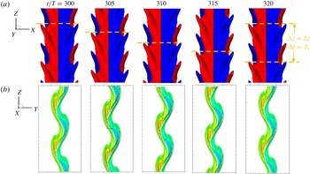
The T-mode (travelling-wave mode) is characterised by a V-shaped vortex distribution in the spanwise direction, which was also named a chevron-shaped pattern by Elston et al. (Reference Elston, Blackburn and Sheridan2006). The T-mode is developed when the flow is fully developed, as demonstrated in figure 16 at
 $(KC,\unicode[STIX]{x1D6FD})=(5,34)$
for both
 $L_{z}=4\unicode[STIX]{x03C0}$
and
 $8\unicode[STIX]{x03C0}$
. The V-shaped vortex structures travel downwards along the spanwise direction at a certain speed
 $u_{z}^{\unicode[STIX]{x1D714}_{z}}=L_{z}/T_{s}$
and have both
 $z$
translation–reflection symmetry (3.8) and
 $z$
travelling–translation symmetry, defined by
 $$\begin{eqnarray}\displaystyle & \displaystyle Z_{t}:\unicode[STIX]{x1D714}_{z}(x,y,z,t)=\unicode[STIX]{x1D714}_{z}(x,y,z-u_{z}^{\unicode[STIX]{x1D714}_{z}}\unicode[STIX]{x0394}t,t+\unicode[STIX]{x0394}t). & \displaystyle\end{eqnarray}$$
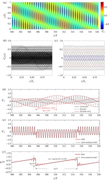
The spatio-temporal variation in
 $C_{L}(z,t)$
for a T-mode flow is in the form of a travelling wave downwards along the spanwise direction from left to right, as shown in figure 17(a). Spatially, no fixed node and peak positions are identifiable (figure 17
b). The spanwise variation in the flow field is mainly induced by a single-mode instability (
 $m=1$
), as shown in figure 9, because the 3-D instabilities at the other wavenumbers are negligible.
Demonstration of the T-mode at
 $(KC,\unicode[STIX]{x1D6FD})=(5,34)$
for
 $L_{z}=4\unicode[STIX]{x03C0}$
with two spanwise repetitions. (a) Top view for the iso-surface of
 $\unicode[STIX]{x1D714}_{z}=\pm 0.15$
and (b) slice view at
 $x=2$
of the flow field (vorticity
 $-0.5\leqslant \unicode[STIX]{x1D714}_{z}\leqslant 0.5$
is shown in colour contour, and
 $-0.15\leqslant \unicode[STIX]{x1D714}_{x}\leqslant 0.15$
is shown as contour lines).

Investigation of sectional lift coefficient in the T-mode, following the same case as figure 12. (a) A local contour of sectional lift coefficient (
 $C_{L}(t,z)$
). (b) The transient sectional
 $C_{L}(z)$
. (c) The component of
 $m=1$
of (b) from
 $t/T=300$
to
 $320$
at a fixed phase of streamwise oscillation
 $t_{0}/T=0$
(- - - -, blue), 0.1 (– ⋅ – ⋅ –, red), 0.15 (——) and 0.4 (- - - -, green). (d) The transient spatial amplitude of the lift coefficient contributed by the cosine part and sine part with envelope curves. (e) The overall transient spatial amplitude of the lift coefficient at
 $m=1$
, extracted from DNS and predicted using the model. (f) The comparison of transient spanwise phase angle
 $\unicode[STIX]{x1D711}$
of sectional
 $C_{L}(z)$
at
 $m=1$
between the results extracted from DNS and the prediction using the semi-analytical model.

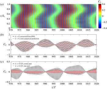
Similarly, a spatial Fourier transform was performed on the sectional lift force in the form of (3.12), and the results are shown in figure 17(d). As shown, the phase of the secondary period of the sine part
 $C_{L}^{s}$
lags
 $\unicode[STIX]{x0394}\unicode[STIX]{x1D6FC}=\unicode[STIX]{x03C0}/2$
behind the cosine part
 $C_{L}^{c}$
(similar to that in figure 6
 $b$
) and can be approximated using the semi-analytical model (3.6)
 $$\begin{eqnarray}\displaystyle & \displaystyle C_{L}^{c}(t)=\unicode[STIX]{x1D6F9}(\unicode[STIX]{x1D70F})\text{cos}(2\unicode[STIX]{x03C0}f_{s}t+\unicode[STIX]{x1D6FC}_{c0}), & \displaystyle\end{eqnarray}$$
 $$\begin{eqnarray}\displaystyle & \displaystyle C_{L}^{s}(t)=\unicode[STIX]{x1D6F9}(\unicode[STIX]{x1D70F})\text{cos}(2\unicode[STIX]{x03C0}f_{s}t+\unicode[STIX]{x1D6FC}_{s0}), & \displaystyle\end{eqnarray}$$
where
 $\unicode[STIX]{x1D6F9}$
is proportional to the streamwise phase variation function
 $\unicode[STIX]{x1D6F9}^{\ast }$
as shown in figure 6(d), while
 $\unicode[STIX]{x1D6FC}_{c0}$
and
 $\unicode[STIX]{x1D6FC}_{s0}$
are the initial phases of
 $C_{L}^{c}$
and
 $C_{L}^{s}$
, and the phase difference can be expressed as
 $$\begin{eqnarray}\displaystyle & \displaystyle \unicode[STIX]{x1D6FC}_{c0}=\unicode[STIX]{x1D6FC}_{s0}+{\displaystyle \frac{\unicode[STIX]{x03C0}}{2}}. & \displaystyle\end{eqnarray}$$
Therefore, the sectional
 $C_{L}(z)$
can be decoupled by substituting (3.18)–(3.20) into (3.12),
 $$\begin{eqnarray}\displaystyle \displaystyle C_{L}(t,z) & = & \displaystyle C_{L}^{c}(t)\text{cos}(k\unicode[STIX]{x03C0}z)+C_{L}^{s}(t)\text{sin}(k\unicode[STIX]{x03C0}z)\nonumber\\ \displaystyle & = & \displaystyle \unicode[STIX]{x1D6F9}(\unicode[STIX]{x1D70F})[\text{sin}(2\unicode[STIX]{x03C0}f_{s}t+\unicode[STIX]{x1D6FC}_{s0})\text{cos}(k\unicode[STIX]{x03C0}z)+\text{cos}(2\unicode[STIX]{x03C0}f_{s}t+\unicode[STIX]{x1D6FC}_{s0})\text{sin}(k\unicode[STIX]{x03C0}z)]\nonumber\\ \displaystyle & = & \displaystyle (C_{L}^{A})^{\prime }\text{sin}[k\unicode[STIX]{x03C0}z+\unicode[STIX]{x1D719}(t)]=C_{L}^{A}\text{cos}[k\unicode[STIX]{x03C0}z+\unicode[STIX]{x03C0}/2+\unicode[STIX]{x1D719}(t)],\end{eqnarray}$$
where
 $\unicode[STIX]{x1D713}(t)$
is determined by
 $$\begin{eqnarray}\displaystyle & \displaystyle \text{tan}\unicode[STIX]{x1D719}(t)={\displaystyle \frac{\text{sin}(2\unicode[STIX]{x03C0}f_{s}t+\unicode[STIX]{x1D6FC}_{s0})}{\text{cos}(2\unicode[STIX]{x03C0}f_{s}t+\unicode[STIX]{x1D6FC}_{s0})}}=\text{tan}(2\unicode[STIX]{x03C0}f_{s}t+\unicode[STIX]{x1D6FC}_{s0}). & \displaystyle\end{eqnarray}$$
Because of the nature of the tangent function, the phase angle can only be expressed discontinuously:
 $$\begin{eqnarray}\displaystyle & \displaystyle \unicode[STIX]{x1D719}(t)=\text{arctan}[\text{tan}(2\unicode[STIX]{x03C0}f_{s}t+\unicode[STIX]{x1D6FC}_{s0})]\in \left(-{\displaystyle \frac{\unicode[STIX]{x03C0}}{2}},{\displaystyle \frac{\unicode[STIX]{x03C0}}{2}}\right), & \displaystyle\end{eqnarray}$$
 $$\begin{eqnarray}\displaystyle & \displaystyle \unicode[STIX]{x1D711}(t)={\displaystyle \frac{\unicode[STIX]{x03C0}}{2}}+\unicode[STIX]{x1D719}(t)={\displaystyle \frac{\unicode[STIX]{x03C0}}{2}}+2\unicode[STIX]{x03C0}f_{s}t+\unicode[STIX]{x1D6FC}_{s0}-J\unicode[STIX]{x03C0}\in (0,\unicode[STIX]{x03C0}). & \displaystyle\end{eqnarray}$$
 $\unicode[STIX]{x1D711}$
is shown in figure 17(f) and compared with the results extracted from DNS. Here,
 $J$
is an integer determined by the floor or the ceiling of the rounding function
 $$\begin{eqnarray}\displaystyle & \displaystyle J=\left\lfloor 2f_{s}t+{\displaystyle \frac{\unicode[STIX]{x1D6FC}_{s0}}{\unicode[STIX]{x03C0}}}+{\displaystyle \frac{1}{2}}\right\rfloor =\left\lceil 2f_{s}t+{\displaystyle \frac{\unicode[STIX]{x1D6FC}_{s0}}{\unicode[STIX]{x03C0}}}-{\displaystyle \frac{1}{2}}\right\rceil . & \displaystyle\end{eqnarray}$$
Hence, the time-dependent coefficient
 $C_{L}^{A}(t)$
can be expressed as
 $$\begin{eqnarray}\displaystyle & \displaystyle C_{L}^{A}=(-1)^{J}\unicode[STIX]{x1D6F9}(\unicode[STIX]{x1D70F}), & \displaystyle\end{eqnarray}$$
which is consistent with the result extracted from DNS directly and shown in figure 17(e). The angular frequency of
 $\unicode[STIX]{x1D714}_{s}=2\unicode[STIX]{x03C0}f_{s}=2\unicode[STIX]{x03C0}/T_{s}=0.325$
is obtained by a linear fitting.
Investigation of sectional lift coefficient in the ST-mode, following the same case as figure 12. (a) A local contour of sectional lift coefficient (
 $C_{L}(t,z)$
). (b) The transient sectional
 $C_{L}(z)$
. (c) The component of
 $m=1$
of (b) from
 $t/T=180$
to 200 at a fixed phase of streamwise oscillation
 $t_{0}/T=0$
(- - - -, red), 0.05 (– ⋅ – ⋅ –, blue), 0.15 (——) and 0.4 (- - - -, green). (d) The transient spatial amplitude of the lift coefficient contributed by the cosine part and sine part. (e) The overall transient spatial amplitude of the lift coefficient at
 $m=1$
. (f) The transient spanwise phase angle
 $\unicode[STIX]{x1D711}$
of sectional lift coefficient at
 $m=1$
.

3.3.3 Mixed ST-mode
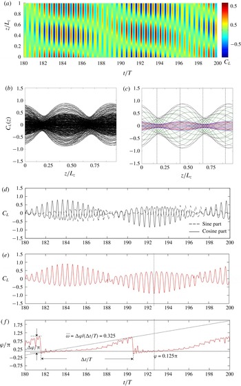
The mixed ST-mode is a transient mode between the S-mode and the T-mode, where vortex flow structures and the sectional
 $C_{L}(z)$
shift from a standing-wave behaviour to a travelling-wave behaviour, as shown in figures 12(
 $a_{\text{iii}}$
) and 18. The ST-mode is still generally a single-mode instability because the
 $C_{L}(z)$
is mainly modulated by the 3-D instability of the leading wavenumber (
 $m=1$
and
 $k=0.5$
in this case). The results are shown in figure 18(c–f), following the same approach as figure 17(c–f). There are two saddle points rather than two node points at approximately
 $z/L_{z}=(0.125+0.25)/2=0.1875$
and
 $(0.625+0.75)/2=0.6875$
and two peak points at
 $z/L_{z}=(0.375+0.5)/2=0.4375$
and
 $(0.875+1)/2=0.9375$
(figure 18
c). This mode appears when the amplitudes of the cosine part and sine part grow unequally in amplitude and the phase difference between them ranges from
 $\unicode[STIX]{x03C0}/2$
to
 $\unicode[STIX]{x03C0}$
(figure 18
d). The sectional lift force forms into a standing–travelling-wave pattern such that its amplitude variation with respect to the temporal phase of the secondary period (figure 18
a–c) is between the standing wave (figure 15
a–c) and the travelling wave (figure 17
a–c). Figure 18(f) shows that the sectional
 $C_{L}(z)$
is more similar to a standing wave with a spatial phase angle of
 $\unicode[STIX]{x1D711}=0.125\unicode[STIX]{x03C0}$
when its temporal amplitude is large, which explains the position of the saddle and peak points by substituting
 $\unicode[STIX]{x1D711}=0.125\unicode[STIX]{x03C0}$
into (3.10) and (3.11). The averaged angular frequency
 $\overline{\unicode[STIX]{x1D714}}_{s}=0.345$
is slightly larger than that of a pure travelling wave
 $\unicode[STIX]{x1D714}_{s}=0.325$
.
3.3.4 X-mode
A typical X-mode obtained through a numerical simulation with
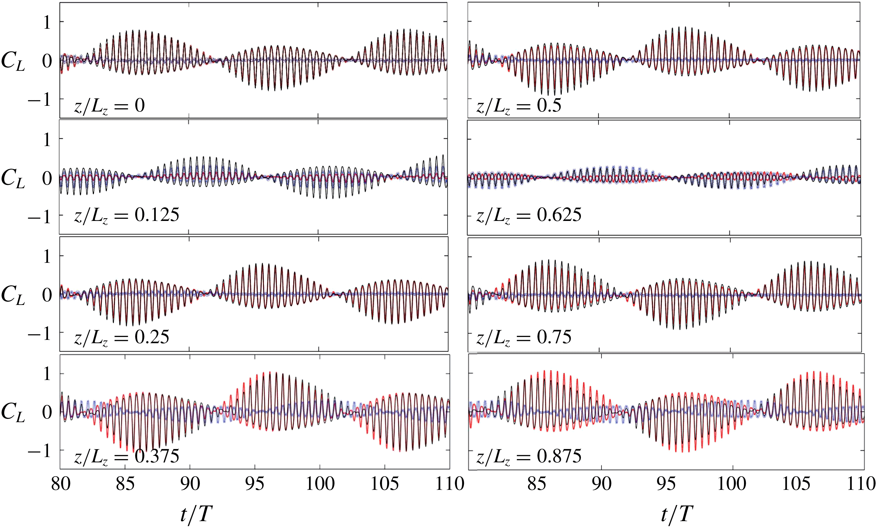
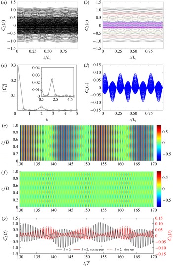
 $L_{z}=8\unicode[STIX]{x03C0}$
is shown in figure 19, and this mode was first observed by Tatsuno & Bearman (Reference Tatsuno and Bearman1990) (figure 19). The spanwise vortex tubes tilt away from the cylinder on both sides of the centre of the X-pattern at approximately
 $z/L_{z}=0.375$
. The three-dimensionality is identified through the coalescence and bifurcation of streamlines in figure 19(b), which agrees well with the photograph of dye streaklines shown in figure 19(c). The
 $z$
-slices of the flow pattern show that the vortex pattern varies greatly from
 $z/L_{z}=0$
to 0.625, whereas it varies rather slightly from
 $0.75\leqslant z/L_{z}\leqslant 1$
.
As determined from the Floquet analysis, there is only one unstable 3-D eigenmode at
 $k=0.5$
(
 $m=1$
) for
 $(KC,\unicode[STIX]{x1D6FD},L_{z})=(5,34,4\unicode[STIX]{x03C0})$
, but there are three discrete unstable modes for
 $L_{z}=8\unicode[STIX]{x03C0}$
at
 $k=0.25$
, 0.5 and 0.75 (
 $m=1$
, 2 and 3). Their linear evolution or nonlinear interaction results in spanwise modulation of the vortex pattern and of
 $C_{L}(z)$
, which differs from those modes discussed previously.
Following the same method of analysis, the transient sectional
 $C_{L}(z)$
of the X-mode is given in figure 20(a), which appears to be a combination of the features exhibited by the S-, T- and mixed ST-modes: (i) the pattern at
 $0\leqslant z/L_{z}\leqslant 0.5$
is similar to the mixed ST-mode for the saddle point, (ii) the pattern at
 $0.5\leqslant z/L_{z}\leqslant 0.75$
is similar to the S-mode for the node point and (iii) the pattern at
 $0.75\leqslant z/L_{z}\leqslant 1$
resembles the T-mode for the
 $z$
travelling–translation symmetry (3.17).
The spectrum of the mean magnitude of the lift coefficient shown in figure 20(d) suggests that the spatio-temporal modulations of the 3-D instability at
 $m=1$
(
 $k=0.25$
) and
 $m=2$
(
 $k=0.5$
) are mainly responsible for the patterns observed in figure 19(a–c). The X-mode is well developed at
 $t/T=80$
when the mean amplitudes at
 $k=0.5$
and 0.75 are approximately 30 % and 15 % of that at
 $k=0.25$
, respectively. Thus, only the components of
 $k=0.25$
and 0.5 are given in figure 20(b,c). For each of them, the sectional
 $C_{L}(z)$
forms into a standing-wave pattern or a slightly mixed standing–travelling-wave pattern. The four nodes of
 $C_{L}(z)$
of
 $m=2$
are located at
 $z/L_{z}=0$
, 0.25, 0.5 and 0.75.
The overall and decoupled sectional
 $C_{L}(z)$
at 8 equi-spaced sectional slices are plotted in figure 21. The components of
 $m=1$
and
 $m=2$
are overall in phase at
 $z/L_{z}=0.125$
but anti-phase at
 $0.625$
. The peak of the lift at
 $z/L_{z}=0.375$
is larger than that at
 $0.875$
due to the different phase lags between the components of
 $m=1$
and
 $m=2$
.
Demonstration of X-mode at
 $(KC,\unicode[STIX]{x1D6FD},L_{z})=(5,34,8\unicode[STIX]{x03C0})$
. (a) The top view iso-surface of
 $\unicode[STIX]{x1D714}_{z}=\pm 0.15$
, (b)
 $\unicode[STIX]{x1D714}_{z}$
contour and streamlines at
 $y=0$
[
 $(x,z)$
-plane], (c) experimental streaklines at
 $KC=4.4$
and
 $\unicode[STIX]{x1D6FD}=50.1$
by Tatsuno & Bearman (Reference Tatsuno and Bearman1990), and (d) cross-sectional slices of
 $\unicode[STIX]{x1D714}_{z}$
contour [
 $(x,y)$
-plane].

Investigation of 3-D instability of the X-mode at
 $(KC,\unicode[STIX]{x1D6FD},L_{z})=(5,34,8\unicode[STIX]{x03C0})$
. (a) Overall transient sectional
 $C_{L}(z)$
. (b) The temporal mean spectrum of
 $C_{L}(z)$
. (c,d) The component of
 $C_{L}(z)$
by Fourier mode at (c)
 $m=1$
(
 $k=0.25$
) and (d)
 $m=2$
(
 $k=0.5$
). (e–g) The local contours with respect to (e) the overall
 $C_{L}(t,z)$
, and (f) the component of
 $m=1$
and (g)
 $m=2$
.

The sectional lift coefficient at different slices from
 $z/L_{z}=0$
to 0.875: ——, overall 3-D result; - - - - (red), component of
 $m=1$
; *** (blue), component of
 $m=2$
.

Modal decomposition of X-mode at
 $(KC,\unicode[STIX]{x1D6FD},L_{z})=(5,34,8\unicode[STIX]{x03C0})$
shown by
 $\unicode[STIX]{x1D714}_{z}$
contours. (a) The 2-D component, (b) cosine and (c) sine components at
 $m=1$
, and (d) cosine and (e) sine components at
 $m=2$
. The corresponding Fourier basis is shown below.

For a better understanding of this pattern, visualisations of decoupled Fourier modes are shown in figure 22. The 2-D component (
 $m=0$
) generally has
 $K_{x}$
symmetry, whereas the cosine and sine Fourier coefficients at
 $m=1$
break the symmetry and resemble a mirror of each other with a different sign. Apart from these, the two Fourier modes are still similar to their counterparts in the S-mode for
 $L_{z}=4\unicode[STIX]{x03C0}$
and the Floquet eigenmode, which further indicates that the flow would be in the S- or the mixed ST-mode if only the 3-D instability at the leading wavenumber existed. A significant difference between the cosine and sine parts is observed for Fourier coefficients at
 $m=2$
, where a clear
 $K_{x}$
asymmetry of both parts is observed. Generally, the X-mode is governed by 3-D instabilities with at least two wavenumbers, which result in spatial and temporal modulations of the primary and secondary instabilities. Consequently, this mode has not been observed in cases where
 $k=0.5$
is the lowest wavenumber of the 3-D instability (
 $m=1$
).
3.3.5 U-mode
The U-mode is observed as
 $\unicode[STIX]{x1D6FD}$
is further increased from the upper bound of the X-mode. The nomenclature is borrowed from Yang & Rockwell (Reference Yang and Rockwell2002), where a unidirectional oblique direction throughout the span was reported. Thus, the overall
 $C_{L}(z)$
acting on the cylinder is no longer insignificant as in the S- or T-modes. It dominates in the spectrum of the mean amplitude of
 $C_{L}(z)$
. An example of the U-mode flow pattern is given in figure 12(c) and figure 23, which are obtained at
 $(KC,\unicode[STIX]{x1D6FD},L_{z})=(5,36,4\unicode[STIX]{x03C0})$
.
Investigation of sectional lift coefficient in the U-mode at
 $(KC,\unicode[STIX]{x1D6FD},L_{z})=(5,36,4\unicode[STIX]{x03C0})$
. (a) Transient sectional
 $C_{L}(z)$
. (b)
 $C_{L}(z)$
distinguishably shown at fixed streamwise oscillation phase
 $\unicode[STIX]{x1D70F}=0$
(——, magenta), 0.1 (
 $\cdots \cdots$
, red), 0.15 (——), 0.25 (- - - -, blue) and 0.4 (- - - -, green). (c) The spectrum of mean absolute value of lift coefficient with inset showing the 3-D components.
 $(d)$
The component of
 $m=4$
(
 $k=2$
) of (a). (e,f) The contour of (e) overall and (f) the component of
 $m=4$
(
 $k=2$
) of
 $C_{L}(z,t)$
. (g) Comparison of the amplitude of the Fourier component of
 $C_{L}(z)$
at
 $k=0$
(2-D) and 2, where different scales are indicated on the left and right vertical axes, respectively.

A comparison of instantaneous
 $\unicode[STIX]{x1D714}_{z}$
contours between the 2-D component and sine component at
 $m=4$
for the U-mode at
 $(KC,\unicode[STIX]{x1D6FD},L_{z})=(5,36,4\unicode[STIX]{x03C0})$
through modal decomposition.

Figure 23(a,b,e) shows that sectional
 $C_{L}(z)$
is significantly different from those of other modes because of a more spatially universal
 $C_{L}(z,t)$
(figure 23
e). Figure 23(c) shows that the 3-D instability peaks at
 $k=2$
(
 $m=4$
), which belongs to
 $B_{\text{II}}$
, and the instability at
 $k=0.5$
in
 $B_{\text{I}}$
is much weaker than its counterpart at
 $\unicode[STIX]{x1D6FD}=34$
due to the strong 2-D instability at
 $\unicode[STIX]{x1D6FD}=36$
. In addition, the component of
 $C_{L}(z)$
induced by the strongest 3-D instability at
 $k=2$
is also clearly different from those induced by 3-D instability of lower wavenumber in
 $B_{\text{I}}$
(e.g. figure 14
c and figure 20
c,d) for the break of reflection symmetry about
 $C_{L}(z)=0$
, and the positive and negative
 $C_{L}(z)$
alternately peaks along the axial direction (23
d,f). The amplitude of the 3-D component reaches the maximum when the amplitude of the 2-D component reaches the minimum (figure 23
g), which leads to the waviness in the contour of overall
 $C_{L}(z)$
. Figure 23(g) also indicates that the secondary period of the component at
 $k=2$
is half of that of the 2-D component because it does not flap with respect to
 $0$
, and its sine part is well correlated with the cosine part despite the former one being approximately 20 % larger than the latter. The existence of relatively steady node and peak points in figure 23(d) can be well explained through an analysis similar to (3.9)–(3.16). In addition, the non-flapping feature of the lift coefficient of the component at
 $k=2(m=4)$
can be qualitatively understood by the comparison of the corresponding instantaneous vorticity contours shown in figure 24. The
 $\unicode[STIX]{x1D714}_{z}$
contours at
 $m=0$
possess a temporal–reflection symmetry as
 $\unicode[STIX]{x1D714}_{z}(x,y,z,t)=-\unicode[STIX]{x1D714}_{z}(x,-y,z,t+T_{s}/2)$
, while those at
 $m=4$
possess an inverse temporal–reflection symmetry as
 $\unicode[STIX]{x1D714}_{z}(x,y,z,t)=\unicode[STIX]{x1D714}_{z}(x,-y,z,t+T_{s}/2)$
. The temporal variations in lift at
 $m=0$
and
 $4$
can be described by
 $C_{L}(t)=-C_{L}(t+T_{s}/2)$
and
 $C_{L}(t)=C_{L}(t+T_{s}/2)$
, respectively.
As shown in § 3.2, the U-mode was also observed in the simulation results obtained at
 $(KC,\unicode[STIX]{x1D6FD},L_{z})=(5,34,16\unicode[STIX]{x03C0})$
in figure 11, which is demonstrated by the results obtained in the last 50 periods of the simulation in figure 25. Although the simulation has not reached equilibrium, the 2-D component prevails in the spectrum of lift coefficients (figure 9), and the 3-D components for
 $k\geqslant 0.375$
have diminished. The 2-D component is not as stable as the result of the 2-D simulation (see figure 7), presumably due to the influence of low-wavenumber instabilities.
Demonstration of the U-mode using sectional lift coefficient at
 $(KC,\unicode[STIX]{x1D6FD})=(5,34)$
for
 $L_{z}=16\unicode[STIX]{x03C0}$
. (a) The contour of sectional
 $C_{L}(z)$
. (b) The 2-D component (
 $k=0$
) of DNS and semi-analytical result, which is predicted by
 $C_{L}=\unicode[STIX]{x1D6F9}(\unicode[STIX]{x1D70F})[\text{cos}(\unicode[STIX]{x1D6FC})+m]$
with
 $m=0.13$
. (c) The cosine and sine part of
 $C_{L}$
of the 3-D component of
 $k=0.125$
.

The variation in the 2-D component (
 $k=0$
) for
 $t/T>600$
(figure 11
b) breaks the spatio-temporal symmetry of the secondary period, which can be expressed by the trace of the lift coefficient:
 $$\begin{eqnarray}\displaystyle & \displaystyle C_{L}(t)=-C_{L}(t+T_{s}/2). & \displaystyle\end{eqnarray}$$
Both the amplitude and period of the secondary oscillation are different (figure 25 b), and the amplitude difference can be approximated by
 $$\begin{eqnarray}\displaystyle & \displaystyle C_{L}(t)=\unicode[STIX]{x1D6F9}(\unicode[STIX]{x1D70F})[\text{cos}(\unicode[STIX]{x1D6FC})+m], & \displaystyle\end{eqnarray}$$
where the extent of asymmetry increases with the increase in the absolute value of
 $m$
, which can be determined by
 $$\begin{eqnarray}\displaystyle & \displaystyle {\displaystyle \frac{(C_{L})_{max}}{(C_{L})_{min}}}={\displaystyle \frac{1-m}{1+m}}. & \displaystyle\end{eqnarray}$$
An approximation of
 $m=0.13$
leads to a good comparison with that by DNS, as shown in figure 25(b). Meanwhile, the variation in the leading 3-D component (
 $k=0.125$
) is modulated by the 2-D component since its amplitude reaches its peak when the amplitude of the 2-D component reaches its minimum (figure 25
c). Similar to the case of the S-mode, the cosine and sine parts are always of opposite signs, with the amplitude of the cosine part being larger than that of the sine part.
Note that the first and second examples of the U-mode are different in terms of mechanism, which leads to distinctive phenomena. The first case at
 $\unicode[STIX]{x1D6FD}=36$
results from the linear superposition of the dominating 2-D instability and weak 3-D instability at higher
 $k$
values. Meanwhile, the second case for
 $L_{z}=16\unicode[STIX]{x03C0}$
is attributable to nonlinear interactions of 2-D instability and 3-D instability at the lowest wavenumber (
 $k=0.125$
) for the following reasons: (i) this phenomenon was not observed by 2-D DNS over 700 cycles for the same
 $KC$
and
 $\unicode[STIX]{x1D6FD}$
; (ii) there is a fixed phase difference between the secondary oscillations of sectional
 $C_{L}(z)$
of
 $k=0$
and 0.125 after
 $t/T\sim 500$
, despite the different eigenfrequencies according to linear stability analysis; and (iii) the decrease in the amplitude of the 2-D instability is synchronous with the increase in the amplitude of the 3-D instability of
 $k=0.125$
after
 $t/T\sim 500$
(figure 11
b).
3.4 Hysteresis phenomenon
The final issue discussed here is the discrepancy about the transition boundary from regime A to regime C (as shown in figure 1) between physical model tests (Tatsuno & Bearman Reference Tatsuno and Bearman1990), DNS and Floquet stability analysis (Elston et al.
Reference Elston, Sheridan and Blackburn2004). To determine the reason for this discrepancy, additional 2-D DNS are performed with different initial conditions: successive initialisations by (i) increasing
 $\unicode[STIX]{x1D6FD}$
and (ii) decreasing
 $\unicode[STIX]{x1D6FD}$
from
 $\unicode[STIX]{x1D6FD}=30$
to 34 with
 $\unicode[STIX]{x0394}\unicode[STIX]{x1D6FD}=0.2$
. Each simulation lasts for 300 flow cycles to obtain equilibrium results. The amplitudes of the lift obtained by using different initial conditions are shown in figure 26(a), in which a hysteresis loop between
 $\unicode[STIX]{x1D6FD}=31.4$
and 33.2 by different initial conditions is observed. The symmetry breaking occurs at approximately
 $\unicode[STIX]{x1D6FD}=32.4$
in the case of increasing
 $\unicode[STIX]{x1D6FD}$
, which is consistent with the result of the Floquet analysis because the initial perturbation has been minimised by successively increasing the
 $\unicode[STIX]{x1D6FD}$
from the
 $K_{x}$
symmetric state. The regime C flow extends to approximately
 $\unicode[STIX]{x1D6FD}=31.4$
by decreasing
 $\unicode[STIX]{x1D6FD}$
, where perturbations with finite amplitudes are introduced. The above results confirm that the transition from regime A to regime C is subcritical. The discrepancy about the transition boundary from regime A to regime C reported in the literature is likely caused by the subcritical nature of the transition.
The subcriticality of the 3-D instability was suggested by Elston et al. (Reference Elston, Blackburn and Sheridan2006) and is demonstrated by comparing the results of the Floquet analysis and the single-mode stability analysis in § 3.1 of this study. A further trial is conducted via a single-mode stability analysis at a fixed parameter point of
 $(KC,\unicode[STIX]{x1D6FD},k)=(5,32,0.25)$
from a series of different initial conditions, which are the fully developed single-mode flow fields obtained at
 $KC=5,k=0.25,30\leqslant \unicode[STIX]{x1D6FD}\leqslant 35$
. Figure 26(b) shows that the strength of the kinetic energy of the 3-D instability depends on the initial condition, demonstrating the subcritical nature of the bifurcation.
Investigation of hysteresis phenomenon. (a) Hysteresis loop by amplitude of the lift coefficient of 2-D DNS at
 $KC=5$
with successive initialisations by increasing
 $\unicode[STIX]{x1D6FD}$
and decreasing
 $\unicode[STIX]{x1D6FD}$
. (b) Single-mode 3-D simulation at
 $(KC,\unicode[STIX]{x1D6FD},k)=(5,32,0.25)$
with different initial conditions of fully developed flow at
 $KC=5$
with
 $\unicode[STIX]{x1D6FD}$
ranging from 30 to 35 (as indicated by the horizontal axis). (c,d) The iso-surface
 $\unicode[STIX]{x1D714}_{z}=\pm 0.25$
of full 3-D DNS at
 $(KC,\unicode[STIX]{x1D6FD},L_{z})=(5,31,8\unicode[STIX]{x03C0})$
from (c) zero initial condition and (d) a fully developed flow field (at
 $\unicode[STIX]{x1D6FD}=36$
). The 2-D component (
 $m=0$
) and cosine part of
 $m=1$
of (d) are plotted in (e) and (f), respectively.

Following the same approach, 3-D simulations are conducted with two different initial conditions at
 $(KC,\unicode[STIX]{x1D6FD},L_{z})=(5,31,8\unicode[STIX]{x03C0})$
. The critical
 $\unicode[STIX]{x1D6FD}$
identified by the Floquet analysis and the experiment at
 $KC=5$
are
 $\unicode[STIX]{x1D6FD}_{cr,F}=32$
and
 $\unicode[STIX]{x1D6FD}_{cr,E}=30$
, respectively. The flow initiated with a zero initial condition evolves into regime A (figure 26
c) and that with the fully developed flow at
 $\unicode[STIX]{x1D6FD}=36$
remains in regime C after 200 cycles (figure 26
d). The flow is almost uniform in the spanwise direction (figure 26
b) with minor perturbations that are detectable by plotting the vorticity coefficients (very small values) at
 $m=1$
, as shown in figure 26(e,f).
4 Conclusions
Regime C flows around an oscillating circular cylinder have been numerically investigated by employing Floquet analysis and direct numerical simulations (DNS). The main findings are summarised below.
(i) The band of 3-D instability at low wavenumber emanating from
 $k=0$
has been detected by the Floquet analysis. The 3-D instabilities appear almost simultaneously with or even slightly before the appearance of 2-D instability. The complex-conjugate Floquet multiplier
 $\unicode[STIX]{x1D707}=|\unicode[STIX]{x1D707}|\text{exp}(\pm \text{i}\unicode[STIX]{x1D714}T)$
obtained from the Floquet analysis confirms the existence of a secondary period
 $T_{s}$
(and frequency
 $f_{s}$
), which can be determined by the angular frequency of
 $\unicode[STIX]{x1D714}_{s}=2\unicode[STIX]{x03C0}/T_{s}=2\unicode[STIX]{x03C0}f_{s}$
. The secondary frequency decreases with increasing
 $\unicode[STIX]{x1D6FD}$
and
 $k$
.
(ii) In 3-D DNS, the minimum wavenumber
 $k_{min}$
of 3-D instabilities that can be resolved is inversely proportional to
 $L_{z}$
as
 $k_{min}=2\unicode[STIX]{x03C0}/L_{z}$
. Instabilities with wavenumbers lower than
 $k_{min}$
can only be resolved by increasing
 $L_{z}$
. Since regime C flow is very sensitive to low-frequency instabilities, it is extremely challenging to achieve a spatial convergence in 3-D DNS simulations. Temporally, a 2-D or 3-D instability with a certain wavenumber can be suppressed by the other dominating instability. The simulation with a cylinder of
 $L_{z}=16\unicode[STIX]{x03C0}$
demonstrated that the competition and nonlinear interaction between the 2-D instability (
 $k=0$
) and the leading 3-D instability (
 $k=0.125$
) would take a long time to reach an equilibrium state (if it even exists). Although not all 3-D instabilities at unstable wavenumbers can be fully resolved, the predicted 3-D vortex patterns are nonetheless similar to those observed in the physical experiments because the 3-D instabilities in the first band are approximately the same.
(iii) According to the flow and force features along the span of the cylinder, the regime C flow structures are categorised into five modes, namely, the standing-wave pattern (S-mode), travelling-wave pattern (T-mode), standing–travelling-wave pattern (mixed ST-mode), X-type pattern (X-mode) and U-type pattern (U-mode), each associated with different low-wavenumber instabilities. The S-, T- and mixed ST-modes mainly result from 3-D instabilities of a single wavenumber, whereas the X-mode is related to 3-D instabilities of multiple wavenumbers. The U-mode is mainly due to the dominating 2-D instability.
(iv) Specifically, the S-mode is characterised by a sinuous phase variation of the vortex shedding in the spanwise direction, with fixed node and peak points. The T-mode is characterised by a travelling pattern of vortices along the span. As the name suggests, the mixed ST-mode is a mixture of the S-mode and T-mode. However, the X-mode replaces the S-mode when a longer spanwise length was used in the simulation, where a lower-wavenumber instability than that of the S-mode increases. The U-mode flow occurs at a parameter where 2-D instability is more dominant than any of the 3-D instabilities, leading to a relatively uniform oblique direction of vortex shedding along the span of the cylinder. For this reason, the spanwise-averaged transverse force is no longer trivial, which is different from the features observed in the other four modes.
(v) A semi-analytical model is proposed to estimate the spatio-temporal evolution of the sectional lift coefficient. The model reveals that the S-mode exists because the cosine and sine components of the leading Fourier mode are always the same in amplitude and opposite in sign. The T-mode is attributed to the invariant phase difference of
 $\unicode[STIX]{x03C0}/2$
between the cosine and sine components, while the mixed ST-mode is a transient state between the S- and T-modes. For the U-mode, the amplitude of the 3-D component always reaches its maximum when the amplitude of the 2-D component reaches its minimum.
(vi) The discrepancy between the marginal stability curves of the transition from regime A to regime C obtained from different approaches is discussed. A hysteresis phenomenon is found in both 2-D and 3-D DNS simulations. This result suggests that the bifurcation from regime A to regime C is subcritical in nature. This is attributed to the discrepancy of the marginal curves obtained by the Floquet stability analysis, DNS and the experiments reported in the literature.
Acknowledgements
The authors would like to acknowledge the support from the National Key R&D Program of China (Project ID: 2016YFE0200100). The first author would like to express sincere thanks to the University of Western Australia for the SIRF Scholarship provided to support this study. The fourth author would like to acknowledge the support of the Australian Research Council through DECRA Schemes (DE150100428). This work was supported by resources provided by the Pawsey Supercomputing Centre with funding from the Australian Government and the Government of Western Australia. The authors would like to thank Dr J. R. Elston for providing his thesis for reference.
Appendix. Model validation
Validation of the selection of interpolant order
 $N_{p}$
and the number of time slices
 $N_{t.s}$
used to reconstruct the base flow for stability analysis is shown in figure 27(a,b). The tests were conducted at
 $(KC,\unicode[STIX]{x1D6FD})=(5,34)$
, the results of which are extensively reported in this study. Three
 $N_{p}$
values were checked, and the differences between
 $N_{p}=8$
and 9 are negligible, which suggests that the selected
 $N_{p}=8$
is sufficient to produce converged results on the 2-D mesh. However, the Floquet analysis is not sensitive to
 $N_{t.s}$
, as the results obtained from 32 and 128 time slices are almost equivalent. Therefore,
 $N_{t.s}=64$
is selected because it is sufficient to accurately characterise the base flow. In addition, the results of the Floquet analysis have been validated against Elston et al. (Reference Elston, Blackburn and Sheridan2006) qualitatively and quantitatively and show great consistency, although the results are not detailed here.
Convergence results for model validation. The comparison of the magnitude of the Floquet multiplier
 $|\unicode[STIX]{x1D707}|$
for different (a) interpolant orders
 $N_{p}$
and (b) time slice numbers
 $N_{t.s}$
at
 $(KC,\unicode[STIX]{x1D6FD})=(5,34)$
with respect to different wavenumbers
 $k$
. (c) The comparison of the mean spectrum of
 $C_{L}(z)$
for different spanwise resolutions
 $N_{z}$
at
 $(KC,\unicode[STIX]{x1D6FD},L_{z})=(5,36,4\unicode[STIX]{x03C0})$
with (d) a close-up view around the peak wavenumber
 $k=2$
.

Figure 27(c,d) presents the convergence test on the spanwise resolution
 $N_{z}$
at
 $(KC,\unicode[STIX]{x1D6FD})=(5,36)$
for
 $L_{z}=4\unicode[STIX]{x03C0}$
by calculating the mean amplitude of the spectrum from FFT analysis on the lift coefficient. Three
 $N_{z}$
values were considered, and the spectra all reach maximum at non-zero wavenumber
 $k=2$
. In addition, the results from
 $N_{z}=32$
and 64 are consistent for a relative difference less than 1 %. Therefore, a conservative selection of spanwise resolution
 $N_{z}=64$
is made for the present study to strike a balance between accuracy and efficiency.