





Impact Statement
Separation zones of open-channel bifurcations have traditionally been represented as closed and two-dimensional; recent studies suggest the presence of open, three-dimensional (3-D) helical recirculation patterns. However, experimental evidence remains scarce due to flow complexity and reliance on two-dimensional observations. Here, we use particle tracking velocimetry to measure the time-averaged 3-D velocity field in a simplified bifurcation geometry. All examined configurations exhibit an open separation zone with no evidence of closed, two-dimensional recirculation. Instead, two distinct helical patterns emerge, governed by the width-to-depth aspect ratio
 $B/h$
, with a threshold near
 $B/h \approx 4$
: in shallow flows, a vertical-axis helix drives ascending recirculation from bed to free surface; in deeper flows, the axis bends from vertical to streamwise, creating a more complex motion. In both patterns, an ‘entrance gate’, a confined near-bed region close to the intersection, controls flow entry into the separation zone, with escape occurring near the surface or at mid-depth. These findings challenge the closed-zone paradigm and offer new insights for flow management in natural and artificial channels.
1. Introduction
Open-channel bifurcation flows consist of one inlet and two outlet channels. Such flows occur ubiquitously in natural and artificial hydraulic networks. Within river environments, bifurcation flows typically occur in deltas (Coffey & Shaw Reference Coffey and Shaw2017; Zou et al. Reference Zou, Zhang, Li, You and Liu2025), just upstream of islands, or at localised water intakes on watercourses for agricultural use or nuclear power plants (Neary et al. Reference Neary, Sotiropoulos and Odgaard1999). Bifurcation flows can also occur in artificial configurations, such as combined storm overflows or at three street intersections in flooded urban areas (Fagour et al. Reference Fagour, Proust and Mignot2024; Rivière et al. Reference Rivière, Travin and Perkins2014).
In both artificial and natural bifurcation flows, the issue of mass transport is of major importance. For example, sediment transport in rivers can change riverbed shapes (Calderón et al. Reference Calderón, Hamad and Escobar-Ortiz2025; Herrero et al. Reference Herrero, Bateman and Medina2015) and affect aquatic life (Best et al. Reference Best, Rhoads, Rice, Roy and Rhoads2008). Similarly, transporting scalars such as micro-pollutants during a flood event can cause several risks to human health (Fagour et al. Reference Fagour, Proust and Mignot2024). Debris transport, ranging from floating wood to urban waste, can block waterways and damage hydraulic structures. Understanding these transport dynamics is therefore crucial for environmental and engineering strategies (Ruiz-Villanueva et al. Reference Ruiz‐Villanueva, Bodoque, Díez‐Herrero, Eguibar and Pardo‐Igúzquiza2013; Yuan et al. Reference Yuan, Wan, Tang, Yan, Qiu and Gualtieri2025; Zou et al. Reference Zou, Zhang, Li, You and Liu2025).
Given the diversity of bifurcation geometries encompassing various angles, branch alignments, section geometries, slopes, bathymetry, types of banks (anthropogenic or vegetated), presence of a flood plain, etc., laboratory studies generally model these bifurcations in a very simplified form, following the foundational work of Bulle (Reference Bulle1926). These simplified geometries are characterised by a straight main open-channel connected to a perpendicular lateral branch. Both channels typically have rectangular sections of the same width, vertical smooth side walls and a horizontal bed. Despite their relative simplicity, these configurations have been the subject of numerous studies over the past century, most of which have been summarised by Alomari et al. (Reference Alomari, Yusuf, Ali and Ghazali2016), Gumgum (Reference Gumgum2025) and Ibrahim et al. (Reference Ibrahim, Ibrahim and Khan2020).
This flow is characterised by several three-dimensional (3-D) flow structures arising from the sharp upstream corner at the entrance of the lateral channel, which gives rise to a flow separation. Inertia deflects the flow towards the opposite wall, creating a low-velocity zone called the ‘separation’ zone along the inner wall. Within this separation zone (SEZ), a so-called ‘recirculation’ motion develops. Part of the flow reverses upstream, performing a revolution before leaving towards downstream. The fluid thus circulates within a large cell, classically referred to as the ‘recirculation zone’ in the literature. The terms ‘separation zone’ and ‘recirculation zone’ are often used as interchangeable terms in the literature, while having a distinct meaning, as shown in the study of an open-channel confluence by Jin et al. (Reference Jin, Ramos, Mignot, Rivière and De Mulder2023).
Traditional representations of the SEZ in the scientific literature consist of a closed semi-elliptical region that separates at the upstream edge and reattaches to the inner wall of the lateral channel (Gumgum Reference Gumgum2025; Mignot et al. Reference Mignot, Doppler, Rivière, Vinkovic, Gence and Simoens2014; Neary et al. Reference Neary, Sotiropoulos and Odgaard1999). This zone exhibits increasing length and width towards the free surface. In addition, the pioneering study by Law (Reference Law1965) showed a monotonically decreasing length-to-width ratio of the SEZ as a function of the lateral to upstream discharge distribution ratio (Kasthuri & Pundarikanthan Reference Kasthuri and Pundarikanthan1987; Lakshama Rao et al. Reference Lakshama Rao, Sridharan and Yahia Ali Baig1968; Shettar & Keshava Murthy Reference Shettar and Keshava Murthy1996). In both studies, the flow within this closed zone is usually described as being two-dimensional (2-D; with no vertical motion) and of infinite residence time, which could induce a potential trapping zone for particles. Finally, in this simplified representation, a secondary flow of streamwise axis is located near the outer wall of the lateral channel. Barkdoll et al. (Reference Barkdoll, Ettema and Odgaard1999) showed that these secondary flows depend on the lateral to upstream discharge ratio (
 $R_q$
).
Many numerical and experimental studies have sought to describe in more detail the shape of the separation zone and the corresponding recirculation flow (RF). Shettar & Keshava Murthy (Reference Shettar and Keshava Murthy1996) depicted the SEZ as a closed region in all measured flow configurations. However, it should be noted that these results are obtained through a 2-D horizontal approach, using numerical simulations averaged over the water depth. Conversely, by analysing the orientation of experimental velocity fields at different altitudes (near the bed, at mid-depth and near the surface), Neary & Odgaard (Reference Neary and Odgaard1993) showed an inhomogeneity along the vertical axis of the separation zone of the lateral channel. This result motivated the conduct of topological studies in 3-D. These studies indicated that the flow separation zone is not closed (Ramamurthy et al. Reference Ramamurthy, Qu and Vo2007). In addition, the presence of three-dimensional helical flow structures in the SEZ is characterised by numerous streamlines following a complex movement (Neary et al. Reference Neary, Sotiropoulos and Odgaard1999). It involves multiple revolutions around a vertical axis, starting from an area near the bed and going up to the free surface, before escaping downstream in the near-free-surface layer. This 3-D recirculation flow suggests that the separation zone is an open zone in certain flow conditions.
More recently, the numerical study by Momplot et al. (Reference Momplot, Lipeme Kouyi, Mignot, Rivière and Bertrand-Krajewski2017) also challenged the classical model of a closed separation zone with a 2-D recirculation flow. The authors proposed a typology of recirculation flow based on two main flow types: the standard closed separation zone with a 2-D recirculation flow, called 3-D closed recirculation, and an open separation zone presenting a three-dimensional helical flow, called 3-D helical recirculation, very similar to the observations of Neary et al. (Reference Neary, Sotiropoulos and Odgaard1999). According to the authors, this helical RF could be observed in bifurcations with low width-to-water depth ratio and high Froude numbers (
 $Fr=Q_u/\sqrt {B^2gh^3}\,$
, where
 $Q_u$
is the discharge in the upstream branch,
 $h$
is the water depth,
 $B$
is the channel width and
 $g$
is standard gravity). However, this typology was established from numerical simulations and observations only, and no detailed experimental study measuring three-dimensional velocity fields has yet confirmed or challenged it. In particular, the transition criterion proposed by Momplot et al. (Reference Momplot, Lipeme Kouyi, Mignot, Rivière and Bertrand-Krajewski2017) and the physical mechanism underlying this transition remain to be experimentally validated.
Many other free surface flows exhibit flow separation zones with complex recirculation flows. The first example is the lateral cavity flow, a free surface flow of limited velocity located along the side of a river or coastal flow, producing velocities of an order of magnitude lower than the characteristic velocity of the flow. Numerous experimental and numerical studies revealed that the recirculation flow is 3-D with limited, yet not negligible, vertical motions. It therefore does not present a zone of infinite residence time for a particle (Engelen et al. Reference Engelen, Perrot-Minot, Mignot, Rivière and De Mulder2021; Navas-Montilla et al. Reference Navas-Montilla, Martínez-Aranda, Lozano, García-Palacín and García-Navarro2021; Sandoval et al. Reference Sandoval, Mignot, Mao, Pastén, Bolster and Escauriaza2019; Tuna et al. Reference Tuna, Tinar and Rockwell2013). Entry of the recirculation flow in the cavity occurs near the bottom, where radial currents concentrate the streamlines towards the centre of the main vortex. The associated streamlines then gain altitude in the water column while gradually moving away from the centre, before escaping near the free surface (Engelen et al. Reference Engelen, Perrot-Minot, Mignot, Rivière and De Mulder2021; Tuna et al. Reference Tuna, Tinar and Rockwell2013). A second example is the junction or confluence of open-channel flow. For such flows, the sharp-edged downstream corner generates a flow separation in the downstream channel and also produces a separation zone located along the inner wall of the channel after the confluence. In the literature, the recirculation flow within a junction is generally represented in 2-D in a plane (Best & Reid Reference Best and Reid1984), with the separation zone delimited by a streamline starting from the downstream corner and reattaching to the inner wall of the downstream channel (as for bifurcation flows; Li et al. Reference Li, Yu, Ma, Wang and Nie2025). However, recent numerical works by Jin et al. (Reference Jin, Ramos, Mignot, Rivière and De Mulder2023) challenged this simplified view. The authors highlight the notable differences between the recirculation zone and the separation zone (often confused in the literature) thanks to clearer definitions and delimitation methods. The use of 3-D streamlines originating from the confluence downstream edge revealed the non-closure of the separation zone in all junction flow configurations. Moreover, the delineating surface – defined as the surface connecting all streamlines starting from the downstream corner of the junction – presents a gap near the bottom. This gap allows for the entry of the flow, generating a 3-D recirculation flow inside the separation zone before escaping downstream in the upper part of the water column. These analogies between lateral cavities, junction flows and bifurcation flows suggest that open, three-dimensional helical recirculation may be a generic feature of free-surface flows past sharp-edged geometries, rather than a peculiarity of any single geometry. In all cases, the aspect ratio between the horizontal extent of the recirculation zone and the water depth appears as a key governing parameter controlling whether the recirculation vortex remains vertically coherent or develops a more complex three-dimensional structure (Engelen et al. Reference Engelen, Perrot-Minot, Mignot, Rivière and De Mulder2021; Jin et al. Reference Jin, Ramos, Mignot, Rivière and De Mulder2023; Tuna et al. Reference Tuna, Tinar and Rockwell2013). This cross-geometry perspective motivates the present study and supports the broader applicability of its findings.
To date, no experimental study has successfully measured the spatially resolved time-averaged 3-D velocity fields in bifurcation flows. The present work thus aims to address this gap in the scientific literature and to assess: (i) whether closed separation zones actually exist in the lateral branch of a bifurcating flow and, more generally, how many recirculation patterns can be observed; (ii) how this recirculating pattern interacts with the secondary currents reported further downstream; and finally (iii) a complementary objective is to generate enriched three-dimensional experimental velocity field benchmarks required for the validation of numerical simulations of such flows.
To the best of the authors’ knowledge, this is the first experimental study to provide spatially resolved, time-averaged 3-D velocity fields in the lateral branch of a bifurcating open-channel flow, using 3-D particle tracking velocimetry (PTV). The corresponding dataset allows a direct assessment of the recirculation topology and its governing parameters, going beyond the two-dimensional or depth-averaged descriptions available in the literature. The paper is organised as follows. Section 2 presents the experimental methods and the dimensional analysis leading to the two key governing parameters (
 $Fr$
and
 $B/h$
) in our highly simplified flow and geometry configurations. Section 3 provides a detailed characterisation of a reference flow configuration. Section 4 performs a parametric study focusing on the role of the governing parameters on the recirculation axis orientation. Finally, Section 5 analyses the recirculation patterns in detail, while Section 6 draws the main conclusions.
2. Methods
2.1. Bifurcation channel
The open channel used in this study was previously used by Ibrahim et al. (Reference Ibrahim, Rivière, Lebouteiller and Mignot2022) and Mignot et al. (Reference Mignot, Cai, Polanco, Escauriaza and Rivière2017). It consists of two straight, transparent, smooth channels made of glass, with the main channel connected to the lateral branch at mid-length, forming a right angle. Both channels have rectangular cross-sections, with a width
 $B = 30\,$
cm. The length of the three branches of this intersection equals
 $L = 2\,$
m (
 $\approx 6.7B$
). The entire set-up is horizontal. The end of each channel is connected to a retention tank with a capacity of
 $0.5\,$
m3, interlinked to form a closed-loop circuit. A pump, immersed in the downstream tank, delivers water to the upstream tank through rigid pipes; the discharge is controlled by a valve, and an electromagnetic flow-meter (Proline Promag 50W Endress Hauser) provides the upstream discharge
 $Q_u$
with a measurement uncertainty
 $\Delta Q = 0.05\,$
L s−1. Once the water reaches the upstream tank, it flows through a honeycomb structure tranquillising the flow and channelising it in one direction. The flow then splits between the downstream and lateral branches to their respective retention tanks. The water collected in the lateral tank is conveyed through another rigid pipe to the downstream tank. This pipe is equipped with a second flow-meter, allowing measurement of the lateral branch discharge
 $Q_l$
(
 $\Delta Q = 0.05\,$
L s−1). Then,
 $Q_d$
can be obtained by mass conservation. The water depth is controlled by adjusting the weir crest downstream of both channels. The water height is measured using an ultrasonic sensor positioned at the midpoint of the lateral channel, one channel width downstream from the intersection. Measurements performed at several locations, including the upstream channel, the separation zone and the vena contracta, showed a maximum relative water depth difference lower than 2%. The free surface elevation, monitored continuously by the ultrasonic sensor, remained constant throughout each acquisition, confirming the steady nature of the mean flow. A schematic representation of the flow circulation and the selected control volume (CV) are shown in Figure 1. The figure also introduces the coordinate system adopted in the present study, whose origin is located at the foot of the upstream edge of the bifurcation, and X and Y axes are respectively aligned with the lateral and downstream channels. This volume includes the entire intersection area (
 $30 \times 30\,$
cm2), a portion of the upstream channel upstream from the upstream corner, as well as a large portion of the lateral channel over
 $120\,$
cm.
Sketch of the experimental bifurcation device. The control volume (CV) is represented by a red dashed line. The hourglass symbol represents the control valve, the rectangles represent the flow meters, and the star indicates the location of the ultrasonic sensor.

Figure 1 Long description
A diagram of an experimental bifurcation device. The diagram includes an upstream tank, a lateral tank, and a downstream tank. The control volume is outlined by a red dashed line. The flow meters are represented by rectangles, and the control valve is indicated by an hourglass symbol. The star marks the location of the ultrasonic sensor. The upstream tank connects to the lateral and downstream tanks, with the flow controlled by valves and measured by flow meters. The distances and dimensions are labeled, with L representing 2 meters and B representing 0.3 meters. The flow rates are denoted as Qu and Ql.
2.2. Particle tracking velocimetry
The detailed characterisation of the flow in the lateral branch requires a 3-D measurement of the flow field, measured via the 3-D-3C PTV method. The whole measurement set-up is located in a closed room, permitting the adjustment and control of the illumination. This illumination is carried out using a pulsed Bernoulli Nd:YAG laser with double cavity length,
 $532\,$
nm wavelength,
 $2 \times 200\,$
mJ power and a frequency of
 $15\,$
Hz. The laser beam, originating from the side of the lateral channel, is split into a 3-D volume by placing two cylindrical lenses of different focal lengths (15 and
 $100\,$
mm) in series oriented perpendicular to each other, allowing a Gaussian illumination distribution of a volume of
 $150 \times 50 \times 15\,\text{cm}^3$
, covering the control volume depicted in Figure 2.
Sketch of the main elements of the experimental set-up with the hydraulic channels in bifurcation arrangement, a camera block positioned under the side channel and an illumination system positioned on the left side of the side channel, allowing an illumination zone shown in green.

The seeding particles are custom-made fluorescent spherical particles elaborated using Mostefaoui et al. (Reference Mostefaoui, Lopez, Mignot and Massardier-Nageotte2024)’s protocol. They consist of
 $100 \pm 20\,{\unicode[Arial]{x03BC}}\mathrm{m}$
diameter particles made of PMMA embedded with Rhodamine B. These particles correspond to Stokes numbers ranging between
 $2\times 10^{-4}$
and
 $4\times 10^{-4}$
in all flows selected, enabling us to consider them as tracers (Xu & Bodenschatz Reference Xu and Bodenschatz2008). A few grams of particles are introduced into the downstream tank, ensuring a homogeneous distribution of tracers after approximately 30 minutes. Image acquisition is performed by a block of four 10-bit cameras designed by LaVision, known as the ‘MiniShaker TR’ system set at a spatial resolution of
 $1984 \times 1264\,$
pixels. These cameras are equipped with
 $8\,$
mm lenses and band-pass filters with a cut-off wavelength of
 $605 \pm 15$
nm, tailored to the maximum emission wavelength of the embedded Rhodamine B particles. The MiniShaker TR system is positioned under the channel at a distance of
 $80\,$
cm below the channel bed, enabling a measurement volume of
 $80 \times 50 \times 20\,\text{cm}^3$
. As the chosen control volume exceeds the maximum dimension of the camera field of view, it is concatenated from two separated fields of view overlapping by 10 cm. The continuity of the time-averaged velocity field across this overlapping region was verified for all flow configurations, confirming the consistency of the two fields of view and the absence of any systematic bias introduced by the concatenation procedure. The image processing is done using the Davis10 software, including the shake-the-box (STB) predictive algorithm developed by LaVision (Schanz et al. Reference Schanz, Gesemann and Schröder2016). All Lagrangian trajectories are obtained by applying the STB algorithm to the thousands of images acquired. The time-averaged Eulerian velocity field is then obtained by applying a binning algorithm over all trajectories, averaging the velocity components from the instantaneous trajectories of the tracked particles across a regular rectangular grid made of cells comprising 24 voxels representing
 $0.5\,$
cm in our channel (allowing a resolution of 300, 60 and approximately 10 cells across, respectively the control volume length, width and height). The averaging process uses a Gaussian weighting function, which depends on the distance between the particle position and the centre of the cell where the Eulerian velocity vector is computed. It should be noted that the near-bed region, within approximately 10% of the water depth
 $h$
from the channel floor, exhibits a higher level of noise in the time-averaged velocity fields. This is primarily attributed to optical reflections and to particle deposition close to the solid boundary, which locally reduces seeding density and the resulting number of resolved velocity vectors, thereby increasing measurement uncertainty in this region. Nevertheless, this does not affect the general shape and orientation of the flow field, which remains consistent with the well-resolved bulk of the flow.
The turbulent fluctuations induced by the channel geometry are not discussed in this study. The statistical uncertainty on the time-averaged velocity field was assessed through two distinct contributions. First, the systematic particle positioning error inherent to the STB tracking algorithm is sub-pixel, as reported by Schanz et al. (Reference Schanz, Gesemann and Schröder2016). Second, the standard deviation of the local velocity fields reaches values of the order of
 $\sigma _U=0.1$
m s−1 within the recirculation zone, where turbulence intensity is highest, while the volume-averaged standard deviation is approximately
 $0.05\,$
m s−1. The statistical uncertainty on the time-averaged velocity, estimated as
 $\sigma _U/\sqrt {N}$
with
 $N \approx 2000$
the number of samples per voxel, is therefore below
 $2 \times 10^{-3}$
m s−1 throughout the measurement volume, which is negligible relative to the mean velocities of interest. This confirms that the time-averaged fields presented hereafter are statistically converged. This convergence was verified through a dedicated convergence study presented in AppendixA. Finally, the large scale 3-D-3C Eulerian time-averaged velocity field measured over
 $L_X \times L_Y \times L_Z = 150\,\text{cm} \times 45\,\text{cm} \times h$
is available for each flow configuration, with
 $h$
the water depth (Figure 1).
2.3. Dimensional analysis
Based on the review in Section 1, this study describes the general time-averaged flow pattern in the lateral channel of the simplified bifurcation geometry with three main key features: the closed or open nature of the separation zone (SEZ closure), linked directly to the recirculation flow pattern, the main axis orientation and the lateral discharge. Under steady flow conditions, those three characteristics are dependent on eleven input dimensional variables as follows:
 \begin{equation} \text{flow pattern} = f(g, \rho , \mu , \sigma , Q_u, Q_d, Q_l, h_u, h_d, h_l, D_{\text{weir}}, B), \end{equation}
where
 $g$
is the standard gravity;
 $\rho$
the fluid density;
 $\mu$
the fluid dynamic viscosity;
 $\sigma$
the air/water surface tension;
 $Q_u$
,
 $Q_d$
and
 $Q_l$
are respectively the upstream, downstream and lateral discharge;
 $h_u$
,
 $h_d$
and
 $h_l$
the corresponding water heights;
 $D_{\text{weir}}$
is the crest height of both weirs (taken equal to each other); and
 $B$
the channel width. Considering the stage-discharge relationship at both weirs,
 $h_d$
and
 $h_l$
can be related to their respective discharges:
 $h_i = f(Q_i, D_{\text{weir}})$
. Furthermore, mass conservation provides a relationship between all three discharges:
 $Q_u = Q_l + Q_d$
. Finally, the momentum balance along the lateral channel allows deriving an additional equation linking the water heights, discharges and crest heights of the lateral and upstream channels (Ramamurthy et al. Reference Ramamurthy, Tran and Carballada1990; Rivière et al. Reference Rivière, Travin and Perkins2011). The seven flow parameters,
 $Q_u$
,
 $Q_d$
,
 $Q_l$
,
 $h_u$
,
 $h_d$
,
 $h_l$
and
 $D_{\text{weir}}$
, can then be reduced to only three key parameters using the four equations stated earlier:
 $Q_u$
(the upstream discharge),
 $Q_l$
(the lateral discharge) and
 $h_l$
(the lateral water height), which is labelled
 $h$
for the remainder of the study.
All remaining eleven parameters involve 3 scales, a length scale,
 $h$
, a mass scale,
 $\rho h^3$
, and a time scale,
 $h^3/Q_u$
. By applying the Vaschy–Buckingham
 $\Pi$
-theorem, the general flow pattern (ratio of outlet discharge, shape of the recirculation zone and axis orientation) in the lateral branch downstream of the bifurcation is a function of four dimensionless parameters:
 \begin{equation} \text{flow pattern} = \phi \left ( Re_h=\frac {4\rho Q_u}{B \mu } , We=\frac {\rho Q_u^2}{B h^2 \sigma }, Fr=\frac {Q_u}{\sqrt {B^2 h^3 g}},\frac {B}{h} \right ). \end{equation}
To simplify the analysis, it was decided to fix the discharge ratio
 $R_q=Q_l/Q_u$
to approximately 50%. In addition, the effect of this parameter was extensively studied by Ibrahim et al. (Reference Ibrahim, Rivière, Lebouteiller and Mignot2022). The present study will focus solely on the closure of the separation zone (SEZ) and its main axis orientation.
Visualisation of width-to-depth aspect ratio and squared Froude number for the 10 flow configurations measured in the present study and indicated by coloured circles. The grey markers pertain to configurations studied numerically by Momplot et al. (Reference Momplot, Lipeme Kouyi, Mignot, Rivière and Bertrand-Krajewski2017), where the squares and triangles correspond to a closed recirculation pattern and a helical recirculation pattern, respectively. The transition proposed by these authors is depicted with a dashed line.

The Weber number (
 $We$
) compares fluid inertia with surface tension effects. When
 $We$
is substantially greater than 1, it indicates that surface tension effects are negligible. Furthermore, this study takes place within the fully turbulent regime (
 $Re_h \gt 10\,000$
), ensuring that the influence of the Reynolds number remains negligible. The two main characteristics, namely, the closure of the separation zone and the recirculation flow main axis orientation, can finally be written as a function of two dimensionless parameters:
 \begin{equation} (\text{SEZ closure, axis orientation}) = \phi (Fr,\,B/h). \end{equation}
2.4. Strategy
Based on the dimensional analysis detailed earlier, the present work aims to assess the influence on the flow pattern of the two governing parameters, namely the aspect ratio (ratio of channel width to water flow depth,
 $B/h$
) and the Froude number (
 $Fr$
). Two independent series of experimental configurations are considered. The first series consists of varying the value of the Froude number of the upstream branch for two fixed values of the aspect ratio
 $B/h=2.95$
and
 $4.17$
. For each value of
 $B/h$
, three flow configurations are studied: one in each topological area as proposed by Momplot et al. (Reference Momplot, Lipeme Kouyi, Mignot, Rivière and Bertrand-Krajewski2017) and the last one just at the interface (Figure 3). The second series consists of varying the aspect ratio
 $B/h$
for seven configurations by keeping the Froude number constant
 $Fr=0.215 \pm 0.05$
: F1 for the deepest flow (
 $B/h=2.95$
); F2, F3 and F4 for intermediate flows; and F5 and F6 for shallow flows. It is to be noted that for all flows, the discharge ratio,
 $R_q=Q_l/Q_u$
, is maintained approximately constant at 49 %–53 %. All flow parameters are listed in Table 1. The chosen ranges of Fr and B/h are influenced by experimental limitations. Exploring smaller Froude numbers would require smaller particles to maintain sufficiently small Stokes numbers, at the cost of reduced light scattering, thus requiring a more powerful laser source to maintain a usable signal. However, higher Froude numbers and the corresponding higher velocities would require a higher acquisition rate than what the present laser can provide (15 Hz). Be that as it may, the selected ranges of Fr and B/h are satisfactorily consistent with those explored numerically by Momplot et al. (Reference Momplot, Lipeme Kouyi, Mignot, Rivière and Bertrand-Krajewski2017), allowing a direct comparison of present results with their typology. In Figure 3, the chosen experimental configurations are depicted by coloured circles within the
 $Fr^2$
versus
 $B/h$
space introduced by Momplot et al. (Reference Momplot, Lipeme Kouyi, Mignot, Rivière and Bertrand-Krajewski2017), along with the grey squares indicating a closed recirculation pattern and grey triangles representing a helical recirculation pattern reported by these authors. Furthermore, the transition line between these two patterns, as proposed by the authors, is depicted with a dashed line.
Experimental parameters for all flows measured for the parametric study (i) of the Froude number
 $Fr$
and (ii) of the aspect ratio
 $B/h$
. Flows F1 (blue) and F5 (red) are chosen as common to both parametric studies

Table 1 Long description
The table presents experimental parameters for various flow configurations in a parametric study. It has two series with multiple rows and columns. Column headers include Series, Flow, D_weir (mm), h (mm), Q_u (L s^-1), R_q (-), B/h (-), and Fr (-). Row labels include different flow configurations. Notable trends include varying Froude numbers and aspect ratios across different flows. Flows F1 and F5 are common to both parametric studies. The table lists specific values for each parameter in each flow configuration.
2.5. Main recirculating axis
One objective of this study is to focus on the orientation of the main recirculation axis of the recirculation zone (see Figure 4). Therefore, the proposed method for identifying this principal axis systematically characterises the 3-D shape of the main recirculating axis, regardless of its location, orientation or direction. The approach comprises the following three main steps.
-
(i) The 3-D time-average velocity gradient tensor
 $ \nabla \boldsymbol{U}$
is initially computed in the first horizontal XY plane of index
$ n$
close to the bed (
$ z/h \approx 0$
). Specifically, we look for points where two eigenvectors of
$ \nabla \boldsymbol{U}$
, denoted
$ \boldsymbol{n_{c1}}$
and
$ \boldsymbol{n_{c2}}$
, are associated with two complex conjugate eigenvalues. These two eigenvalues indicate a rotational fluid motion around an axis carried by the remaining eigenvector
$ \boldsymbol{n_r}$
of
$ \nabla \boldsymbol{U}$
, associated with a real eigenvalue.
-
(ii) The intersected position of the main recirculating axis with the search plane then corresponds to the point
$ (x_n, y_n, z_n)$
where the norm
$ \|\boldsymbol{U}(x_n, y_n, z_n)\| = \boldsymbol{U} \cdot \boldsymbol{n_r}$
. We therefore seek
$ (x_n, y_n, z_n)$
such that:
\begin{equation*} \left \{ \begin{aligned} \boldsymbol{U}(x_n, y_n, z_n) \cdot \boldsymbol{n}_{c1} &= 0 ,\\ \boldsymbol{U}(x_n, y_n, z_n) \cdot \boldsymbol{n}_{c2} &= 0 .\end{aligned} \right . \end{equation*}
This system of two equations with two unknowns is solved numerically using the iterative Newton-Raphson method. The initial value
$ (x_0, y_0)$
of this algorithm is chosen to be equal to the position of a 2-D critical point close to the winding of the streamlines in the lowest horizontal (XY) plane. It has been verified that the choice of such an initial position does not influence the result of the present algorithm. -
(iii) Once one point of the recirculation axis is identified, the next point is searched in a plane offset by an increment
$ \Delta d$
along the direction of the eigenvector
$ \boldsymbol{n_r}$
of
$ \nabla \boldsymbol{U}$
and with
$ \Delta d$
defined as half the grid size of the velocity field. The position of the algorithm’s initial guess of this new plane
$ n+1$
is taken as the projection of the previous axis point in the new plane.





Steps (ii) and (iii) are repeated until it is no longer possible to find a solution. This method thus allows for the reconstruction, point by point and plane by plane, of the entire 3-D principal axis of the recirculation flow of our bifurcation flow. Furthermore, despite the low signal-to-noise ratio near the bed, the axis detection algorithm is robust regardless of the initialisation point.
Illustration of the recirculation axis detection algorithm.

Figure 4 Long description
A diagram illustrating the recirculation axis detection algorithm in bifurcation flows. The diagram shows a helical path with an initial guess marked in red and the Newton-Rhapson method marked in magenta. The helical path is surrounded by three vectors labeled n_r, n_c1, and n_c2, representing different directions. The diagram includes a coordinate system with axes labeled e_x, e_y, and e_z. The helical path spirals upward from the base to a point labeled U(x_n, y_n, z_n), indicating the final position. The distance Δd is marked along the z-axis.
3. Description of the reference flow
This section establishes the key concepts and flow structures using the F5 flow (
 $Fr=0.22$
,
 $B/h=4.17$
) as a reference case. The structures defined here, delineating surface, recirculation flow and entrance gate, serve as the analysis framework applied to all ten configurations in the parametric study. All streamlines of the time-averaged Eulerian velocity field used in the present study are computed using the MATLAB streamline function, which implements a fourth-order Runge–Kutta scheme with linear interpolation between grid nodes. The step size was chosen to be 10 % of the grid cell.
3.1. Recirculation flow in the separation zone
The delineating surface (DS) is defined as the surface encompassing all time-averaged streamlines originating from the upstream corner of the intersection over the entire water depth (
 $x/B=y/B=0$
), which constitutes the physical separation point imposed by the geometry; it usually delimits the so-called separation zone (SEZ). Several definitions of the separation zone exist in the literature. It is defined herein as the volume bounded by the delineating surface (DS), the free surface (
 $z/h=1$
), the bed (
 $z/h=0$
) and the inner wall (
 $y/B=0$
) of the lateral branch as proposed by Jin et al. (Reference Jin, Ramos, Mignot, Rivière and De Mulder2023). However, the recirculation flow (RF) is defined by all streamlines coming from the upstream channel and which exhibit at least one revolution around the Z-axis in the lateral channel (thus exhibiting some negative longitudinal velocities
 $U_x\lt 0$
). Finally, the non-recirculation flow (NRF) is defined by all streamlines in the lateral channel that do not recirculate.
Illustration of the different structures of the F5 flow: (a) recirculation flow (RF) formed by all streamlines starting from the upstream channel and performing at least one rotation in the lateral channel are coloured by their elevation
 $z/h$
. The sections bounding this zone, upstream and downstream of the study area, are plotted in dark green. (b) Delineating surface (DS) consisting of streamlines starting from the upstream corner coloured based on their initial relative elevation
 $z_{init}/h$
. (c) Non-recirculation flow (NRF) is composed of all other non-recirculating streamlines entering the lateral channel, they are also coloured by their elevation
 $z/h$
. The surfaces delimiting this zone, upstream and downstream of the study area, are plotted in cyan.

Figure 5 illustrates these different elements for our reference flow. Figures 5a and 5c show respectively the RF and the NRF, with streamlines coloured according to the elevation
 $z/h$
. The cross-section bounding these two zones, upstream (at
 $y/B=-0.4$
) and downstream (at
 $x/B=4$
) of the study area, are plotted in dark green and cyan in Figures 5a and 5c. In Figure 5b, the DS is represented by the streamlines coloured based on their elevation at the upstream edge of the bifurcation
 $z_{\rm init}/h$
. For clarity, the latter are only plotted until they begin their first half-turn (i.e. until the longitudinal velocity
 $U_x$
becomes null before being negative). It should be noted that while the present framework follows the general approach introduced by Jin et al. (Reference Jin, Ramos, Mignot, Rivière and De Mulder2023) for open-channel confluences, slightly different conventions are adopted here. In particular, unlike Jin et al. (Reference Jin, Ramos, Mignot, Rivière and De Mulder2023), the streamlines that originate from the upstream edge in the lower part of the water column, in yellow in Figure 5b, belong to the DS. As reported by Momplot et al. (Reference Momplot, Lipeme Kouyi, Mignot, Rivière and Bertrand-Krajewski2017) and Neary et al. (Reference Neary, Sotiropoulos and Odgaard1999), Figure 5a exhibits a helical motion with a vertical axis of clockwise direction in the SEZ. This structure generates an upward fluid movement, from the bed in the upstream branch (region coloured upstream in dark green in Figure 5a) to the free surface in the lateral branch. The streamlines then exit the study area in the small area delineated in dark green. This analysis reveals that the DS does not reattach to the inner wall (
 $y/B=0$
) of the lateral channel nor to the bed channel, and presents an open surface downstream. The SEZ is thus not a closed zone for our reference flow F5.
The streamlines of the NRF (Figure 5c) can be divided into two categories according to their entry position in the lateral channel and their vertical movement: first, the streamlines located near the higher part of the water column (
 $z/h\gt 0.5$
) stay roughly at the same altitude and parallel to the outer wall (along
 $y/B=1$
); second, streamlines near the bottom of the water column (
 $z/h \lt 0.5$
) follow a more pronounced helical flow along a longitudinal axis and a clockwise direction, approaching the inner wall (
 $y/B=0$
).
In the downstream zone (
 $x/B \gt 2.1$
), the DS delimits the RF from the NRF. This demarcation is particularly visible in the plane
 $x/B=4$
, where the DS is represented by green (Figure 5a) and cyan (Figure 5c) contours. It appears that, in the downstream part of the measurement zone, the volume delineated by the DS and the free surface only contains RF (for all
 $x/B\gt 2.1$
). These observations are highly similar to those made in the numerical study on junction flows by Jin et al. (Reference Jin, Ramos, Mignot, Rivière and De Mulder2023).
3.2. Characteristics of the recirculation flow
Top view representation of recirculating streamlines of the F5 flow, whose origin comes from the region of the corner near the upstream (
 $x/B=0$
and
 $y/B=0$
), which presents multiple revolutions (1, 2, 4 and an unknown number of turns) around a vertical axis. These lines are coloured according to their elevation ratio
 $z/h$
.

Figure 6 Long description
Panel A: A line graph shows recirculating streamlines with 1 lap. The x-axis is labeled x/B and the y-axis is labeled y/B. The streamlines are colored according to their elevation ratio, with blue indicating lower elevation and red indicating higher elevation. Panel B: A line graph shows recirculating streamlines with 2 laps. The x-axis is labeled x/B and the y-axis is labeled y/B. The streamlines are colored according to their elevation ratio, with blue indicating lower elevation and yellow indicating higher elevation. Panel C: A line graph shows recirculating streamlines with 4 laps. The x-axis is labeled x/B and the y-axis is labeled y/B. The streamlines are colored according to their elevation ratio, with blue indicating lower elevation and yellow indicating higher elevation. Panel D: A line graph shows recirculating streamlines with more than 4 laps. The x-axis is labeled x/B and the y-axis is labeled y/B. The streamlines are colored according to their elevation ratio, with blue indicating lower elevation and yellow indicating higher elevation.
To illustrate the main structure of the helical RF with a vertical axis for the F5 flow, some of the streamlines are plotted in Figure 6, illustrating a 2-D top view representation of four recirculating streamlines, coloured according to their elevation
 $z/h$
. These streamlines perform 1, 2, 4 and an unknown number of turns respectively around the main recirculating axis located at
 $x/B \approx 1.25$
. They rise progressively as they undergo multiple revolutions while approaching the vertical recirculation axis.
The streamlines that perform many revolutions (
 ${\gt} 4$
) approach the main recirculation axis closely, where the spatial scales of these recirculation flows are likely smaller than the mesh size of our measured velocity field (
 $0.5\,$
cm). This limitation makes it difficult to estimate the maximum number of revolutions a streamline completes within the RF. However, all computed streamlines reach a limit of 20 revolutions before transitioning into periodic limit cycles, i.e. following the same path indefinitely, due to the finite spatial resolution of the experimental velocity field.
3.3. Entrance gate to the separation zone
The RF is a helical flow whose streamlines come from the upstream branch (Figure 5a), confined by the delineating surface (DS) at the end of the lateral channel
 $x/B \gt 3$
. This necessarily implies an opening in the DS through which all the recirculating streamlines forming the RF enter this zone. This opening will henceforth be called the ‘entrance gate to the separation zone’.
Figure 7 illustrates the flow pattern with another view angle: (i) the DS is plotted in greyed transparency, with the parts in contact with the bed and the free surface represented by dotted lines, respectively in blue and light green; (ii) the recirculating streamlines are traced up to the first cancellation of their longitudinal velocity (
 $U_x$
) and thus their first half-turn, and coloured according to their elevation
 $z/h$
as in figure 5a. The discontinuity between the blue and green lines denotes a gap in the volume delineated by the DS, the so-called entrance gate. The definition used in this paper slightly differs from that chosen by Jin et al. (Reference Jin, Ramos, Mignot, Rivière and De Mulder2023), whereas this gap starts from the junction edge. This figure highlights and indicates the longitudinal and transverse extent of the entrance gate of the SEZ, which is very limited (approximately
 $1.5 \lt x/B \lt 2.1$
and
 $0 \lt y/B \lt 0.25$
). It is to be noted that the minimum of external surfaces to the SEZ (vena contracta) is located at the same position as the lift of the DS,
 $x/B=0.8$
. An additional description of the entrance is available in the Appendix A.
Three-dimensional representation of the DS for F5 flow in transparent grey; dotted lines indicate the contacts with the bed (blue) and the surface (green). All recirculating streamlines (RF) are plotted up to their first cancellation of longitudinal velocity (
 $U_x$
) and coloured according to their elevation
 $z/h$
.

Projections of the main recirculation axes on the XZ plane (a) and the XY plane (b) for the flows of the second study (with
 $Fr=0.215 \pm 0.05$
and a varying
 $B/h$
value), F1 to F6.

4. Recirculation axis
The reference flow F5, characterised in the previous section, presents a recirculation pattern with a vertical axis extending from the channel bed to the free surface, identified using the method described in Section 2.5. The recirculation axis for the nine other flows described in Table 1 is now studied in the present section, as a function of the two parameters identified in Section 2.3, namely the aspect ratio
 $B/h$
and the Froude number
 $Fr$
.
Regarding the first series dedicated to the influence of the aspect ratio
 $B/h$
, figures 8a and 8b illustrate respectively the projection of the recirculation axes in the XZ and XY planes, for the flows F1–F6 (i.e. from the deepest to the shallowest) characterised by
 $Fr \approx 0.215$
and
 $B/h$
varying from 3 to 6. Two main orientations of the recirculation axes appear: (i) a mainly vertical orientation (for F5 and F6) for the shallow flows, labelled ‘vertical’ orientation in the sequel; and (ii) a double orientation starting with a vertical orientation from the bed to about mid-depth upstream to a horizontal orientation extending to the downstream end of the lateral branch, for the deepest flows (F1–F4), labelled ‘horizontal’ for the remaining part of this paper. The base of the vertical recirculation axis (at the bed level) moves from
 $x/B=0.2$
, for the deepest flow F1 (presenting a horizontal axis), to
 $x/B=1.45$
for the shallow flow F5 (presenting a vertical axis). It should be noted that, for flow F5, the recirculation axis exhibits a change in orientation at around
 $z/h \approx 0.4$
, transitioning from an upstream-tilted to a downstream-tilted direction above this elevation. This change does not coincide with the region of reduced data quality (mentioned in Section 2.2), which is limited to the two lowermost measurement layers (
 $z/h \lt 0.15$
). This inflection is therefore interpreted as a genuine geometric feature of the recirculation axis rather than a measurement artefact.
Regarding the second series dedicated to the influence of the Froude number
 $Fr$
, figures 9a and 9b illustrate respectively the projection of the recirculation axes in the XZ and XY planes, for the flows {F1, F1’, F1”} characterised by
 $Fr=\{0.151, 0.217, 0.256\}$
with
 $B/h=2.95$
; and {F5, F5’, F5”} with
 $Fr=\{0.220, 0.316, 0.387\}$
and
 $B/h=4.17$
. Consistently with the orientations identified above, flows F1, F1’ and F1” (
 $B/h=2.95$
) retain a horizontal orientation, and flows F5, F5’ and F5” (
 $B/h=4.17$
) retain a vertical orientation, irrespective of
 $Fr$
.
Projections of the recirculation axes in the XZ plane (a) and the XY plane (b) for flows with fixed aspect ratios
 $B/h=\{2.95, 4.17\}$
coloured respectively in shades of blue (F1, F1’ and F1”) and orange (F5, F5’ and F5”).

Figure 9 Long description
Panel A: A scatter plot shows projections of the recirculation axes in the XZ plane. The x-axis is labeled 'x/B' and ranges from 0 to 2.5. The y-axis is labeled 'z/h' and ranges from 0 to 1. The data points are colored in shades of blue and orange, representing different flows (F1, F1', F1'' in blue and F5, F5', F5'' in orange). The plot shows various trajectories of the recirculation axes, with blue points generally following a lower path and orange points showing more vertical movement. Panel B: Another scatter plot displays projections of the recirculation axes in the XY plane. The x-axis is labeled 'x/B' and ranges from 0 to 2.5. The y-axis is labeled 'y/B' and ranges from 0 to 1. Similar to Panel A, the data points are colored in shades of blue and orange. The plot indicates the horizontal spread of the recirculation axes, with blue points showing a more consistent pattern and orange points exhibiting more variation.
For the two values of
 $B/h$
, the variation of the Froude number
 $Fr$
causes a slight displacement of the longitudinal position of the base of the recirculation axis (
 $z/h \approx 0$
), but the influence of
 $Fr$
on the overall shape and orientation of the recirculation axis remains negligible.
Having shown that the recirculation axis orientation is essentially governed by
 $B/h$
, the geometry of this axis is now characterised more systematically by combining the flows of both series. Two main characteristics can be extracted from these axes: (i) the curvilinear axis length
 $L_{\rm ax}$
normalised by the water depth
 $h$
and (ii) the longitudinal position of the axis basis
 $x_{\rm ax}$
normalised by the channel width
 $B$
. Figures 10a and 10b plot these two characteristics as a function of the aspect ratio
 $B/h$
for the ten flows. It should be noted that the length of the axis
 $L_{\rm ax}/h$
was calculated only up to
 $x/B=2.25$
, which is the downstream detection limit of the horizontal recirculation axis of flow F4. The triangular and circular symbols represent, respectively, the flows presenting a vertical and horizontal recirculation axis orientation.
A transition from one recirculation axis orientation to the other can be observed for
 $B/h \approx 4$
(horizontal for F1–F4 and vertical for F5 and F6), as illustrated in Figure 8. This transition can be interpreted as a vertical confinement effect on the recirculation vortex. In shallow flows (
 $B/h \gt 4$
), the water depth is small relative to the channel width. Hence, the recirculation vortex develops primarily in the horizontal plane but is vertically confined by the bed and the free surface. This confinement constrains the vortex axis to remain vertical and forces the recirculating fluid to spiral upward along this axis before escaping near the free surface.
The effect of confinement is often observed in open channel flows, though in different configurations or patterns. For instance, a threshold aspect ratio value has been reported in lateral cavity flows (Mignot et al. Reference Mignot, Barros, Riviere and Escauriaza2026; Rivière et al. Reference Riviere, Garcia, Mignot and Travin2010) and in groyne fields (McCoy et al. Reference McCoy, Constantinescu and Weber2008; Weitbrecht et al. Reference Weitbrecht, Socolofsky and Jirka2008), where a length-to-width ratio value segregates two recirculation cell patterns. Moreover, shallow conditions promote vertically coherent, quasi-2-D horizontal vortices. Conversely, in deeper flows (
 $B/h \lt 4$
), the reduced influence of bed friction and the greater vertical extent allow the initially vertical vortex axis to tilt and reorient progressively towards a streamwise (horizontal) direction downstream. The interaction with the secondary current near the outer wall (
 $y/B=1$
) could also explain such transitions. This behaviour echoes observations in open-channel lateral cavities (Dong & Uchida Reference Dong and Uchida2024) and groynes (McCoy et al. Reference McCoy, Constantinescu and Weber2008), where increasing relative water depth promotes stronger three-dimensional vortex motions.
(a) Dimensionless lengths of the recirculation axis
 $L_{\rm ax}/h$
calculated up to
 $x/B=2.25$
, as a function of the aspect ratio
 $B/h$
for the ten flows characterised in this study. (b) Dimensionless positions of the origin of the recirculation axis
 $x_{\rm ax}/B$
at
 $z/h=0$
. See Figures 9 and 8 for the corresponding colours.

Finally, the aspect ratio
 $B/h$
thus emerges as the dominant parameter governing the recirculation pattern in open-channel bifurcations. A transition between a predominantly vertical recirculation axis (
 $B/h\gt 4$
, shallow flows) and a vertical-to-horizontal bending axis (
 $B/h\lt 4$
, deep flows) occurs at
 $B/h \approx 4$
, at least within the range of discharge ratios and weir heights explored. The Froude number
 $Fr$
, by contrast, has only a marginal influence on the axis orientation. This hierarchy of parameters, with
 $B/h$
as the primary control, constitutes a central finding of the present study. Having established
 $B/h$
as the primary governing parameter of the recirculation axis orientation, the following section examines in detail how this parameter shapes the full 3-D flow structure, including the closure nature of the separation zone, the geometry of the delineating surface, and the secondary flow patterns, by comparing the two representative configurations F1 (
 $B/h \lt 4$
) and F5 (
 $B/h \gt 4$
).
5. Similarities and differences of horizontal and vertical recirculation axis flow patterns
Building on the parametric study of Section 4, which identified
 $B/h$
as the dominant governing parameter and
 $Fr$
as having only marginal influence, this section provides a detailed characterisation of the two recirculation patterns. The first part compares the 3-D flow structures, namely the helical recirculation flow (RF) and the delineating surface (DS) in the lateral branch, presented in Section 3.1 for all six flows F1–F6. The second part focuses on a comparison of the 2-D velocity fields between flows F1 (
 $B/h = 2.95$
, horizontal axis) and F5 (
 $B/h = 4.17$
, vertical axis), taken as representative configurations of the horizontal and vertical recirculation flow patterns, respectively.
5.1. Three-dimensional flow structures
Figure 11 illustrates the RFs for flows F1–F6, and confirms that all recirculation flows present a helical motion of clockwise direction, conveying fluid from the near-bed region of the upstream branch towards a more elevated area in the downstream part of the lateral branch through an upwelling motion. This consistent clockwise rotation and associated upwelling across all six configurations suggests that the bifurcation geometry imposes a preferred rotation direction regardless of the aspect ratio
 $B/h$
. The two patterns differ, however, in the spatial organisation of this helical motion. Flows F1–F4, presenting a horizontal recirculation axis, exhibit a clockwise helix winding around an axis that is initially vertical before tilting to a streamwise direction downstream. However, for flows F5 and F6, the vertical recirculation axis conveys the recirculating fluid upward along the full height of the water column within the SEZ, before it escapes near the free surface with a much weaker helical motion of horizontal axis, further downstream.
Three-dimensional representation of the recirculation flows (RF) of configurations F1–F6. All streamlines are coloured according to their elevation
 $z/h$
. A section of the DS in the YZ plane at
 $x/B=4$
is also illustrated in green.

Figure 11 Long description
Panel F1: A 3D plot shows recirculation flows in configuration F1. The streamlines are colored according to their elevation, ranging from black to yellow. The horizontal axis is labeled x/B, the vertical axis is labeled z/h, and a section of the downstream channel in the YZ plane is illustrated in green. Panel F2: A 3D plot shows recirculation flows in configuration F2. The streamlines are colored according to their elevation, ranging from black to yellow. The horizontal axis is labeled x/B, the vertical axis is labeled z/h, and a section of the downstream channel in the YZ plane is illustrated in green. Panel F3: A 3D plot shows recirculation flows in configuration F3. The streamlines are colored according to their elevation, ranging from black to yellow. The horizontal axis is labeled x/B, the vertical axis is labeled z/h, and a section of the downstream channel in the YZ plane is illustrated in green. Panel F4: A 3D plot shows recirculation flows in configuration F4. The streamlines are colored according to their elevation, ranging from black to yellow. The horizontal axis is labeled x/B, the vertical axis is labeled z/h, and a section of the downstream channel in the YZ plane is illustrated in green. Panel F5: A 3D plot shows recirculation flows in configuration F5. The streamlines are colored according to their elevation, ranging from black to yellow. The horizontal axis is labeled x/B, the vertical axis is labeled z/h, and a section of the downstream channel in the YZ plane is illustrated in green. Panel F6: A 3D plot shows recirculation flows in configuration F6. The streamlines are colored according to their elevation, ranging from black to yellow. The horizontal axis is labeled x/B, the vertical axis is labeled z/h, and a section of the downstream channel in the YZ plane is illustrated in green.
Three-dimensional representation of the delineating surfaces (DS) of flows F1–F6. All streamlines are coloured according to their initial elevation at the upstream corner
 $z_{\rm init}/h$
. The red dotted lines indicate the contact with the bed. A section in the YZ plane of the DS at
 $x/B=4$
is also illustrated in magenta.

Figure 12 compares the DS for all six flows. Consistently with the reference case F5, all DS detach from the bed near
 $x/B \approx 1$
and none reattaches to the inner wall (
 $y/B=0$
), confirming the open nature of the SEZ across all configurations. Downstream, the DS reaches the free surface (for the vertical axis configurations) or winds around itself (for the horizontal axis configurations). Moreover, the streamlines’ winding intensity seems to increase as the aspect ratio
 $B/h$
decreases. A comparison of the non-recirculation flows (NRF) for all six flows is available in appendix.
5.2. Analysis of 2-D velocity flow fields
To complement the 3-D structures described earlier, the 2-D velocity fields in the XY and YZ planes are presented to further characterise the secondary flow patterns observed within the separation zone of the lateral branch.
The following section, therefore, focuses on the study of the dimensionless longitudinal and transverse velocities in the XY and YZ planes for both F1 (deep flow with a horizontal axis orientation) and F5 (shallow flow with a vertical orientation), allowing us to highlight those structures better. Figure 13 shows the horizontal time-averaged velocity fields, together with the corresponding 2-D pseudo-streamlines (streamlines plotted from the 2-D flow field measured at this elevation, rather than a 2-D projection of 3-D streamlines), for both F1 and F5 flows: (a) near the bottom of the channel, about mid-elevation where the streamlines enter the recirculation flow (
 $z/h = 0.15$
); (b) mid-depth (
 $z/h = 0.5$
); and (c) near the free surface (
 $z/h = 0.85$
).
Two-dimensional velocity fields in the XY plane at elevations
 $z/h = \{0.15 , 0.50, 0.85\}$
for flows F1 and F5. The velocity fields represented are coloured according to the dimensionless average streamwise velocity. A magenta isoline also illustrates the zones of zero longitudinal velocity. Pseudo-streamlines are displayed in black.

Figure 13 Long description
Panel A: The first column shows velocity fields for flow F1 at three different elevations (z/h = 0.85, 0.50, 0.15). The velocity fields are colored according to the dimensionless average streamwise velocity, with a color scale ranging from blue to red. A magenta isoline indicates zones of zero longitudinal velocity. Pseudo-streamlines are displayed in black. The x-axis is labeled x/B and ranges from -1 to 4, while the y-axis is labeled y/B and ranges from 0 to 1. Panel B: The second column shows velocity fields for flow F5 at the same elevations. The color scale, magenta isoline, and pseudo-streamlines are consistent with those in Panel A. The x-axis and y-axis labels and ranges are identical to those in Panel A.
Two-dimensional velocity fields in the YZ plane at a longitudinal position
 $x/B = \{0.80 , 2.50\}$
for flows F1 and F5. The velocity fields are coloured according to the dimensionless average transversal velocity. The blue dotted lines designate the intersection of the delineating surface with the YZ section. The cyan square symbols and orange circular symbols represent respectively in these figures, the intersection of the main recirculation axis and the intersection of a secondary flow axis. Pseudo-streamlines are displayed in black.

The velocity fields measured near the bottom of the lateral branch confirm that both flow patterns present a strong transverse flow from outside (near the outer wall, at
 $y/B=1$
) towards the inside of the separation zone (in the direction of the negative
 $Y$
-axis for
 $0.5\lt x/B\lt 3$
). Overall, the shallower flow F5 (with a vertical recirculation axis) generates larger streamwise velocity magnitudes
 $U_x$
than the deeper flow F1 (with a horizontal recirculation axis). At mid-depth, the velocity fields are very similar for both flows: the zone of negative longitudinal velocity extends from
 $x/B=0$
to 2 or 3, with the focus located around
 $x/B \approx 1.2$
corresponding to the location of the main recirculation axis. This similarity at mid-depth explains why depth-averaged or mid-depth-only observations in the literature (e.g. Kasthuri & Pundarikanthan Reference Kasthuri and Pundarikanthan1987; Lakshama Rao et al. Reference Lakshama Rao, Sridharan and Yahia Ali Baig1968; Shettar & Keshava Murthy Reference Shettar and Keshava Murthy1996) did not allow one to distinguish the two recirculation patterns. Indeed, only near-bed and near-surface measurements could reveal such a difference. Additionally, the corner vortex located near the upstream corner and present in the lower part of the water column winds in a direction opposite to that of the main recirculation axis (counter-clockwise). This recirculation, as well as the primary recirculation flow, creates a region of significantly reduced velocity that can give rise to pollutants, particle or sediment trapping phenomena (Calderón et al. Reference Calderón, Hamad and Escobar-Ortiz2025). Finally, the near-free-surface flow fields differ significantly between the two recirculation flow patterns. As seen earlier, the horizontal axis flow pattern generates a strong three-dimensional helical flow starting from the inner wall (
 $y/B=0$
) around
 $x/B \approx 2$
(but coming from lower water depths) and reaching a wider zone located at
 $y/B \approx 0.5$
for
 $0\lt x/B\lt 4$
. Conversely, for the two flows with a vertical axis, the fields near the surface remain similar to the fields at mid-depth and near the bottom, indicating a relative homogeneity over the vertical direction.
Figure 14 presents, for both flow F1 and F5, the 2-D dimensionless time-average velocity fields and corresponding pseudo-streamlines in the YZ sections located for both flows, at longitudinal positions
 $x/B = 0.8$
and
 $x/B = 2.5$
, corresponding respectively to the upstream and downstream ends of the entrance gate of the separation zone. As seen previously, the transverse velocity fields located near the upstream end of the entrance gate (
 $x/B=0.8$
) reveal, for both flows, a strong negative transverse velocity (in pink) located near the bottom of the channel going from the outer wall (
 $y/B=1$
) of the lateral branch (outside the separation zone, materialised by the blue line) towards the inner wall (
 $y/B=0$
, inside the SEZ). These observations are reversed near the free surface (in green). The F1 flow (horizontal recirculation axis) exhibits two co-rotating flows located respectively inside and outside the SEZ, carried respectively by the main and secondary recirculation axes illustrated with cyan squares and orange circles on the figures. Conversely, a single helix, corresponding to the secondary flow axis, is observed for flow F5 (vertical recirculation axis). These observations are consistent with the secondary vortices identified by Neary et al. (Reference Neary, Sotiropoulos and Odgaard1999), namely a longitudinal-axis vortex near the outer wall (
 $y/B=1$
) and a small vertical-axis corner vortex near the upstream edge (
 $x/B=0.4$
and
 $y/B=0.15$
) of the lateral branch. Similar secondary vortices were also reported in several other studies (Calderón et al. Reference Calderón, Hamad and Escobar-Ortiz2025; Gumgum & Cardoso Reference Gumgum and Cardoso2024; Momplot et al. Reference Momplot, Lipeme Kouyi, Mignot, Rivière and Bertrand-Krajewski2017).
Downstream of the entrance gate (
 $x/B=2.5$
), both flows exhibit a unique large-scale longitudinal helical flow covering the majority of the flow section, with its focus point located at the centre of the flow separation zone (delimited by the DS indicated in blue dotted lines). It is to be noted that for flow F1 (and all horizontal-axis flows), the two axes do not merge downstream: the secondary axis (in orange), located originally outside the SEZ, is pushed to the outer wall (
 $y/B=1$
) before disappearing at
 $x/B \in [0.8, 1.2]$
, leaving only the main recirculation axis in the downstream part of the lateral branch. That disappearance happens at the same longitudinal position as the tilting (from a vertical to horizontal orientation) of the main recirculation axis. Conversely, for the flow F5 (and all vertical axis flows), the secondary flow axis is observed all the way to the downstream end of the study area.
6. Discussion and conclusions
This study addressed two fundamental questions regarding the flow patterns in open-channel bifurcations: (1) what are the actual possible shapes of separation zones in the lateral branches of bifurcations, and (2) how do the different 3-D flow structures interact within the whole lateral branch. Using 3-D particle tracking velocimetry metrology, this experimental study successfully characterised the time-averaged 3-D velocity fields in a simplified bifurcation channel. By comparing the delineating surfaces (DS) and recirculation flows (RF), the observations unquestionably demonstrate that all observed flow configurations exhibit an open separation zone, with no evidence of the closed, two-dimensional recirculation patterns described in the earlier literature (Momplot et al. Reference Momplot, Lipeme Kouyi, Mignot, Rivière and Bertrand-Krajewski2017; Neary et al. Reference Neary, Sotiropoulos and Odgaard1999). This suggests that the classification proposed by Momplot et al. (Reference Momplot, Lipeme Kouyi, Mignot, Rivière and Bertrand-Krajewski2017), based on numerical simulations, does not accurately capture the three-dimensional helical structure of the recirculating flow observed in the present work. An alternative classification is therefore introduced based on the following two 3-D helical recirculation patterns: vertical-axis helical recirculation, observed in shallower flows (
 $B/h \gt 4$
), where the recirculation flow ascends from the bed to the free surface; and horizontal-axis helical recirculation, observed in deeper flows (
 $B/h \lt 4$
), where the recirculation axis transitions from vertical (upstream) to horizontal (downstream) (Jin et al. Reference Jin, Ramos, Mignot, Rivière and De Mulder2023). The aspect ratio (
 $B/h$
) emerged as the dominant parameter governing the recirculation pattern, while the Froude number (
 $Fr$
) had only a marginal effect for the present configurations. The transition between these two recirculation forms was identified at
 $B/h \approx 4$
. A key finding of this study is the presence of an ‘entrance gate’, a spatially confined region through which all recirculating streamlines enter the separation zone. Flows with a vertical recirculation axis exhibit a certain homogeneity in the vertical direction, with strong horizontal velocities and weaker vertical velocities, whereas flows with a horizontal recirculation axis demonstrate significant heterogeneity over depth, driven by a strong longitudinal helical flow.
In conclusion, this work challenges the classical depiction of bifurcation flows as closed, 2-D systems, instead revealing the prevalence of open, 3-D helical recirculation flows, already observed in other open-channel flow geometries.
Despite these novel insights, the study acknowledges certain limitations. The analysis was restricted to time-averaged velocity fields, with a reduced signal-to-noise ratio near the walls and the free surface. Additionally, quantitative vortex indicators such as vorticity fields, total vertical turbulent kinetic energy, or shear stresses were investigated. Still, they could not be reliably extracted from the present data set. The near-wall and near-bed regions, precisely where the recirculation structures are most intense, exhibit inherently high noise levels in the measured velocity field due to optical reflections and low seeding density close to those boundaries, despite repeated attempts to use different filtering methods, and could not be retained in the present analysis. Finally, as mentioned in Section 2, the experimental conditions and parameter ranges (
 $Fr$
and
 $B/h$
) were constrained by the experimental facilities. The influence of the flow pattern was also studied over a longitudinal length of 4 channel widths. The experimental facilities did not allow for a more extensive longitudinal study. A further limitation concerns the discharge ratio
 $R_q$
, which was maintained at approximately 50 % throughout all experiments (by choosing equal weir crest elevations at the two outlet channels for each configuration). While this choice was motivated by the need to isolate the effects of
 $Fr$
and
 $B/h$
, and is consistent with the approach of Ibrahim et al. (Reference Ibrahim, Rivière, Lebouteiller and Mignot2022), it raises the question of whether the two identified recirculation patterns, and the transition threshold
 $B/h \approx 4$
, remain valid for significantly different values of
 $R_q$
. It is well established that
 $R_q$
strongly influences the size and shape of the separation zone in the lateral branch (Ibrahim et al. Reference Ibrahim, Rivière, Lebouteiller and Mignot2022; Law Reference Law1965; Neary et al. Reference Neary, Sotiropoulos and Odgaard1999): a higher lateral discharge ratio widens the separation zone and displaces the reattachment point further downstream, which could in principle affect the aspect ratio of the recirculation region and thereby shift the transition threshold. It should be noted, however, that since the delineating surface does not reattach to the inner bank of the lateral branch, the reattachment point cannot be defined, making the length of the separation zone, and consequently the concept of aspect ratio, difficult to define rigorously, as previously noted by Jin et al. (Reference Jin, Ramos, Mignot, Rivière and De Mulder2023). To date, no experimental or numerical study has characterised the 3-D recirculation topology as a function of
 $R_q$
, leaving this as an open question. The present results should therefore be interpreted as established for
 $R_q \approx 50\,\%$
, and assessing the sensitivity of the recirculation patterns to the discharge ratio constitutes a natural and necessary extension of this work.
Yet, these findings provide critical insights for river and sewer network management, particularly in understanding sediment, pollutant and debris transport dynamics in bifurcation flows. In particular, the observed non-closure of separation zones indicates that recirculation regions cannot be systematically treated as isolated or inactive storage areas. Instead, they remain dynamically connected to the main time-averaged flow through the entrance gate, allowing continuous exchange of mass and momentum. On the contrary, for the instantaneous flow, this connection is ensured by the turbulent structures developing along the delineating surface, thus intermittently linking the main flow and the separation zone. Qualitatively, the computed streamlines in both recirculation patterns indicate that the recirculating fluid undergoes multiple revolutions within the SEZ before eventually escaping downstream, suggesting residence times significantly longer (but still limited) than a single flow-through time scale
 $B^2h/Q_u$
. This implies that material entering the separation zone, such as fine sediments, pollutants, or floating debris, may experience prolonged residence before being re-entrained into the main flow, rather than being either permanently trapped or instantaneously flushed. The quantification of this residence time constitutes a key priority for future work. Moreover, the presence of significant vertical mixing further enhances mass exchange by promoting transfers between near-bed and upper flow layers, thereby increasing the three-dimensionality of transport processes and reducing the predictability of one-dimensional transport models commonly used in river networks. As a result, bifurcation zones should be interpreted as dynamic exchange environments where storage and transport processes are to be accounted for, with direct implications for sediment management, pollutant dispersion and maintenance strategies in engineered and natural flow systems.
This study provides novel three-dimensional experimental velocity field benchmark data, particularly useful for the calibration of advanced numerical simulation methods, enabling a deeper exploration of flow features and a better understanding of these transitions. Future research could expand on these results by exploring a broader range of flow conditions and refining measurement techniques to capture near-wall and free-surface dynamics.
Acknowledgements
The authors would like to thank Bjarne Vincent from the Laboratoire of Mécanique des Fluides et d’Acoustique (LMFA) for his invaluable help with 3-D flow visualisation and vortex axis identification.
Data availability statement
The data that support the findings of this study are available from the corresponding author upon reasonable request.
Author contributions
All authors contributed to the conceptualisation, data curation, formal analysis, methodology, validation and visualisation. D.L., N.R. and E.M. supervised the study. The original draft of the manuscript was written by O.M. All authors reviewed and edited all previous versions of the manuscript. All authors read and approved the final manuscript.
Funding statement
This work was carried out thanks to the financial support of the University of Lyon’s LabEx iMUST (ANR-10LABX-0064), created as part of the ‘Programme d’Investissements d’Avenir’ set up by the French government and managed by the ‘Agence Nationale de la Recherche’ (ANR), the funding of a PhD extension grant by EUR H2O’Lyon (ANR-17-EURE-0018), as well as support from INSA Lyon as part of Okba Mostefaoui’s ‘INSA Lyon Environmental Issues’ MESR thesis grant.
Competing interests
The authors declare no conflict of interest.
Ethical standards
This declaration is not applicable.
Appendix A
Verification of the convergence of the measured velocity fields
This Appendix presents the convergence study of the time-averaged Eulerian velocity field for flow F5. The convergence of the three velocity components: longitudinal
 $U_x$
, transverse
 $U_y$
and vertical
 $U_z$
, was assessed near the delineating surface (DS), the area where the turbulence is the strongest. The running time-average of each velocity component is plotted as a function of acquisition time and normalised by its final mean value, so that convergence towards unity indicates statistical stationarity. Figure A1 confirms that all three components reach satisfactory convergence well before the end of the acquisition period.
Convergence verification for flow F5 of the (a) longitudinal
 $U_x$
, (b) transverse
 $U_y$
and (c) vertical
 $U_z$
velocity components as a function of acquisition time, at a point located near the delineating surface (DS). All velocity values are normalised by their respective final mean value.

Complementary analysis of the delineating surface’s entrance gate
Figures A2a and A2b illustrate, respectively in 2-D and 3-D, different cross-sections of the F5 flow’s delineating surface (DS), coloured according to
 $x/B \in [0.4, 2.4]$
, with the dotted portions of the sections corresponding to recirculating streamlines (also shown in green in the 3-D visualisation). The pink surface in Figure A2b represents the 3-D entrance gate of the SEZ, while the hatched area represents an extrapolation of the entrance gate profile towards the bed, where direct measurements are unavailable. As mentioned in Section 3.1, the cross-section at
 $x/B = 0.8$
is the first to present an inflection point near the bottom (Figure A2a), indicating a transverse flow directed from outside the SEZ towards the inner wall (
 $y/B = 0$
).
(a) Transverse sections of the DS of the F5 flow coloured according to
 $x/B \in [0.4, 2.4]$
, with the dotted portions of the sections corresponding to recirculating streamlines. (b) Three-dimensional representation of the DS with the same longitudinal sections. The green part of the DS corresponds to the recirculating streamlines, and the pink surface corresponds to the entrance gate. The hatched region denotes the extrapolated portion of the entrance gate profile towards the bed, where direct measurements are unavailable.

Three-dimensional representation of the non-recirculation flows (NRF) of configurations F1–F6. All streamlines are coloured according to their elevation
 $z/h$
. The downstream sections of the DS are illustrated in cyan at the downstream edge of the study area.

Figure A3 Long description
Panel F1: A 3D plot showing streamlines colored by elevation. The axes are labeled x/B, y/B, and z/h. The streamlines start from the upstream edge and curve towards the lateral channel. Panel F2: A 3D plot similar to Panel F1 but with different streamline patterns. The axes are labeled x/B, y/B, and z/h. Panel F3: A 3D plot with distinct streamline patterns compared to Panels F1 and F2. The axes are labeled x/B, y/B, and z/h. Panel F4: A 3D plot showing streamlines with a different configuration. The axes are labeled x/B, y/B, and z/h. Panel F5: A 3D plot with unique streamline patterns. The axes are labeled x/B, y/B, and z/h. Panel F6: A 3D plot with streamlines differing from the other panels. The axes are labeled x/B, y/B, and z/h.
It must be acknowledged that the entrance gate is located precisely in the near-bed region where measurement quality is lowest (within
 $z/h \lt 0.1$
, as discussed in Section 2). Due to optical reflections and reduced seeding density close to the channel floor, the flow field in this layer presented a reduced signal-to-noise ratio, making a direct reconstruction of the entrance gate in this region unfeasible. Its characterisation therefore relies on the three-dimensional streamlines computed by integration of the time-averaged Eulerian velocity field resolved immediately above this layer, rather than on direct velocity measurements within it. Nevertheless, three converging lines of evidence support the physical reality of this structure: (i) the longitudinal position at which the DS detaches from the bed (
 $x/B \approx 0.8$
) is remarkably consistent across all six flow configurations (F1–F6), regardless of the aspect ratio
 $B/h$
or Froude number
 $Fr$
, suggesting a geometry-driven mechanism rather than a flow-condition-dependent artefact; (ii) all recirculating streamlines, regardless of their starting elevation, trace back to this near-bed region when integrated upstream; and (iii) the strong negative transverse velocity component measured near
 $z/h = 0.15$
in the YZ cross-sections (Figure 14) is fully consistent with an inward flow feeding the separation zone from below. Taken together, these independent observations strongly suggest that the entrance gate is a robust physical feature of the flow, rather than a measurement artefact.

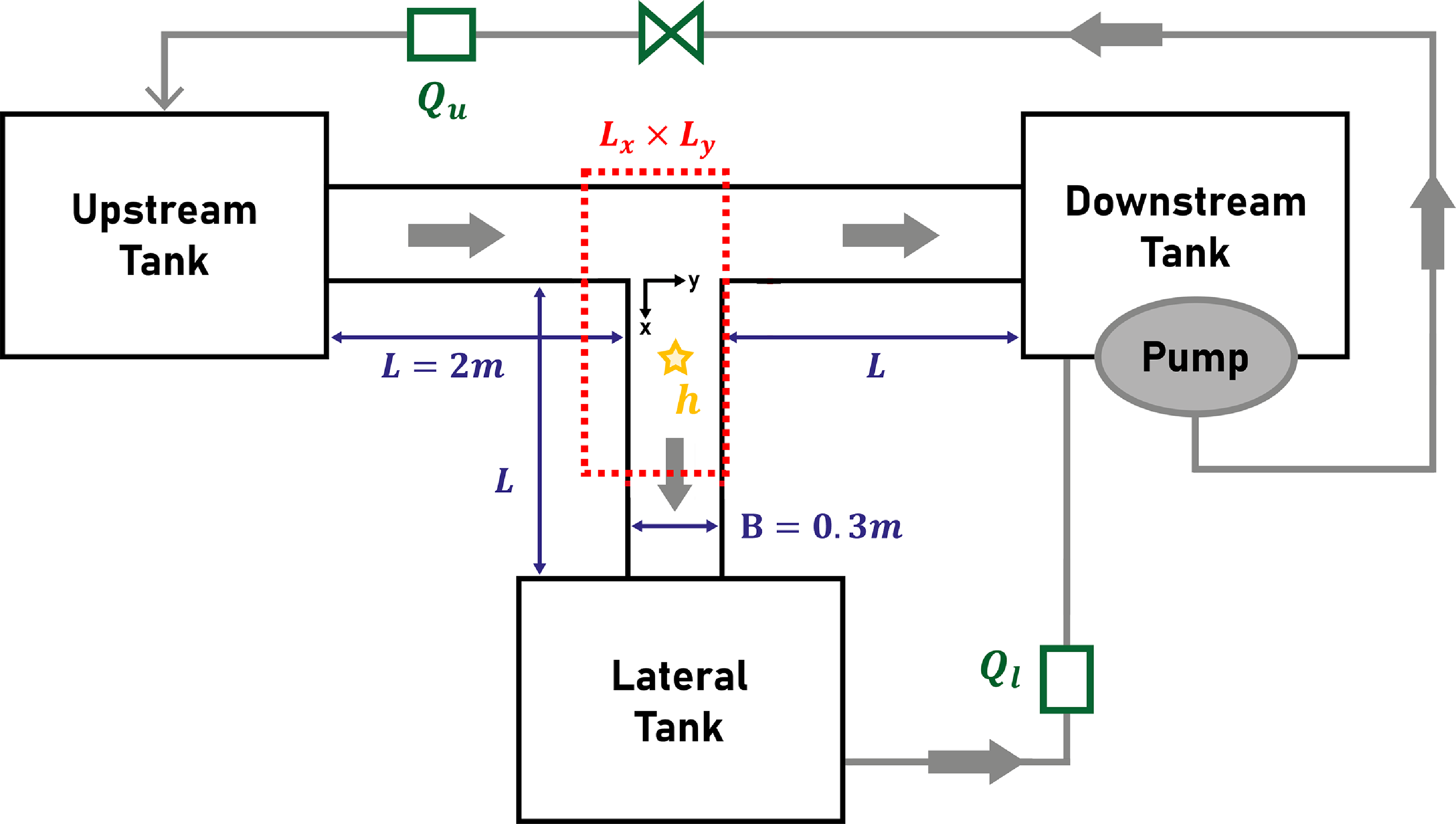
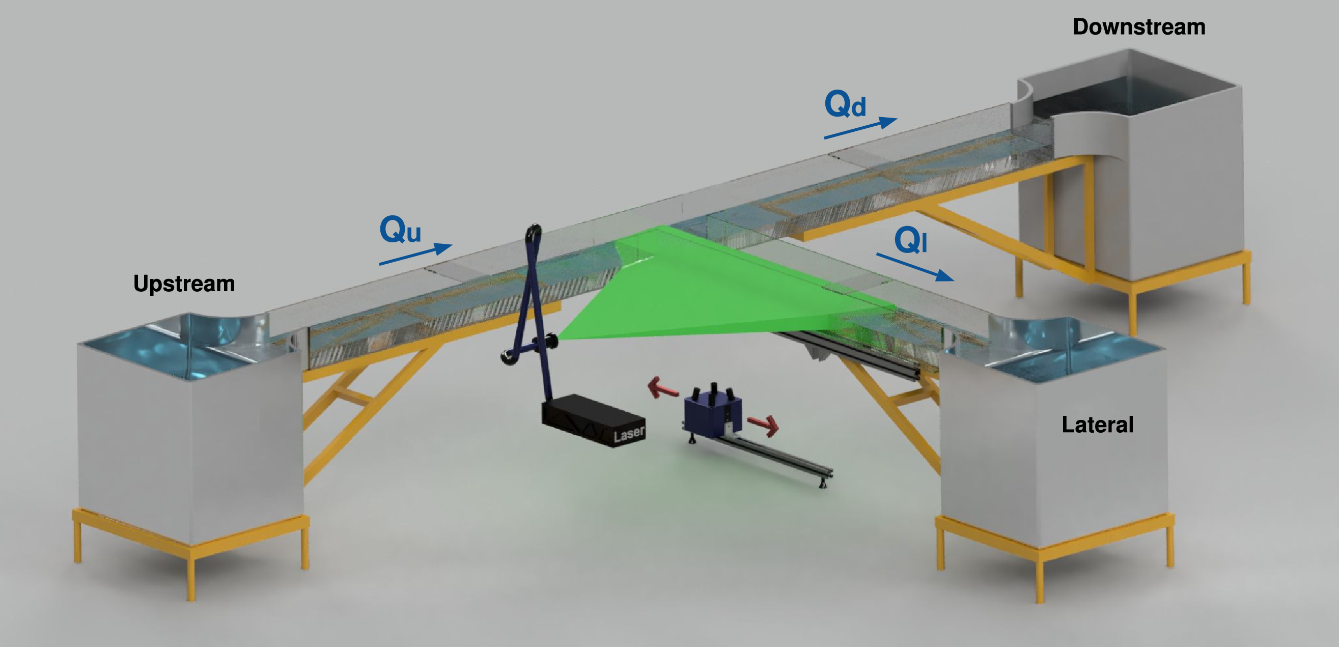
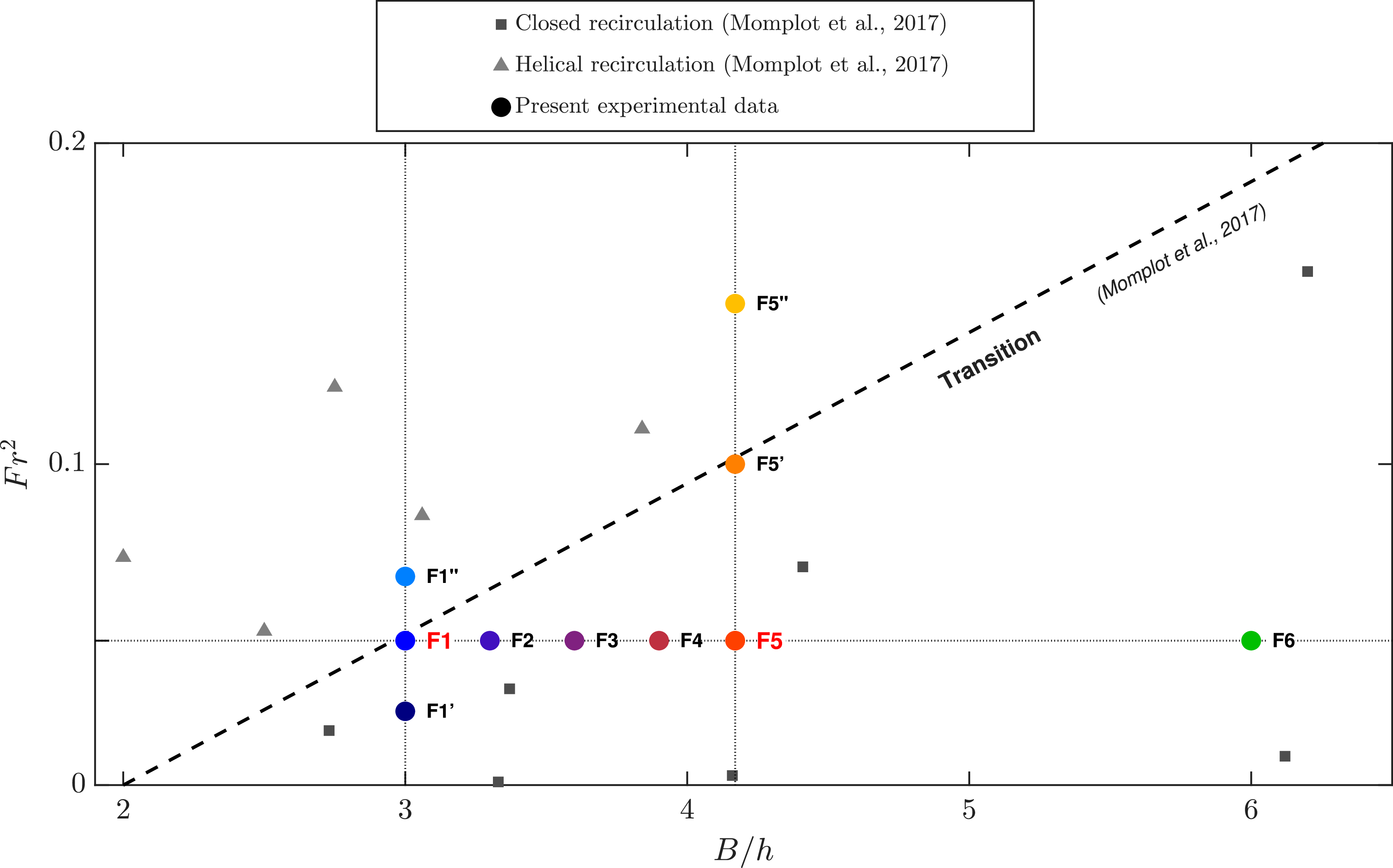
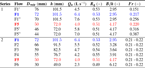
 Fr
 B/h
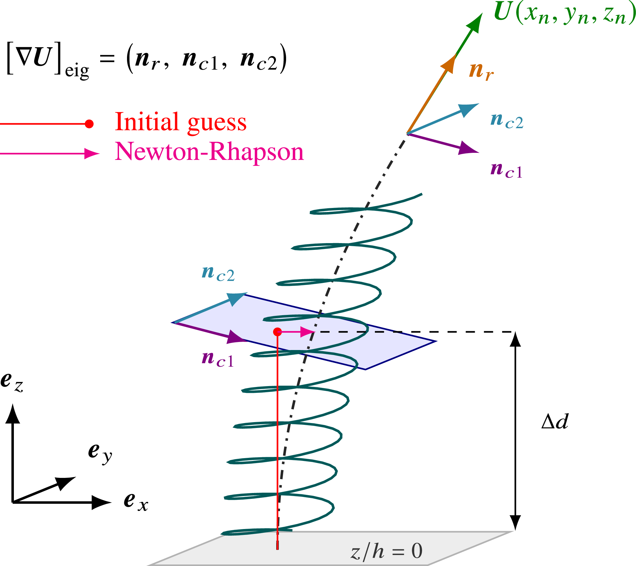
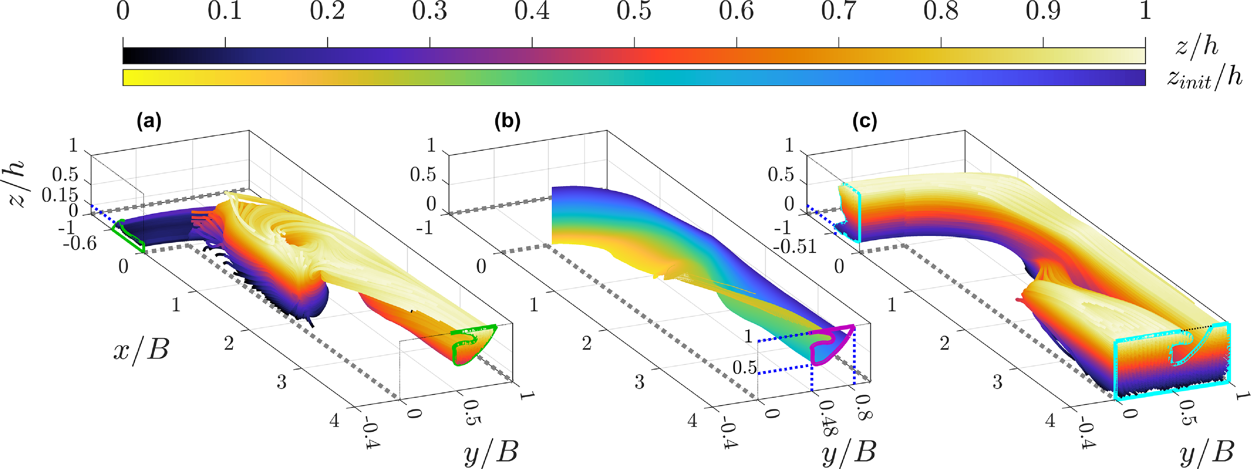
 z/h
 zinit/h
 z/h
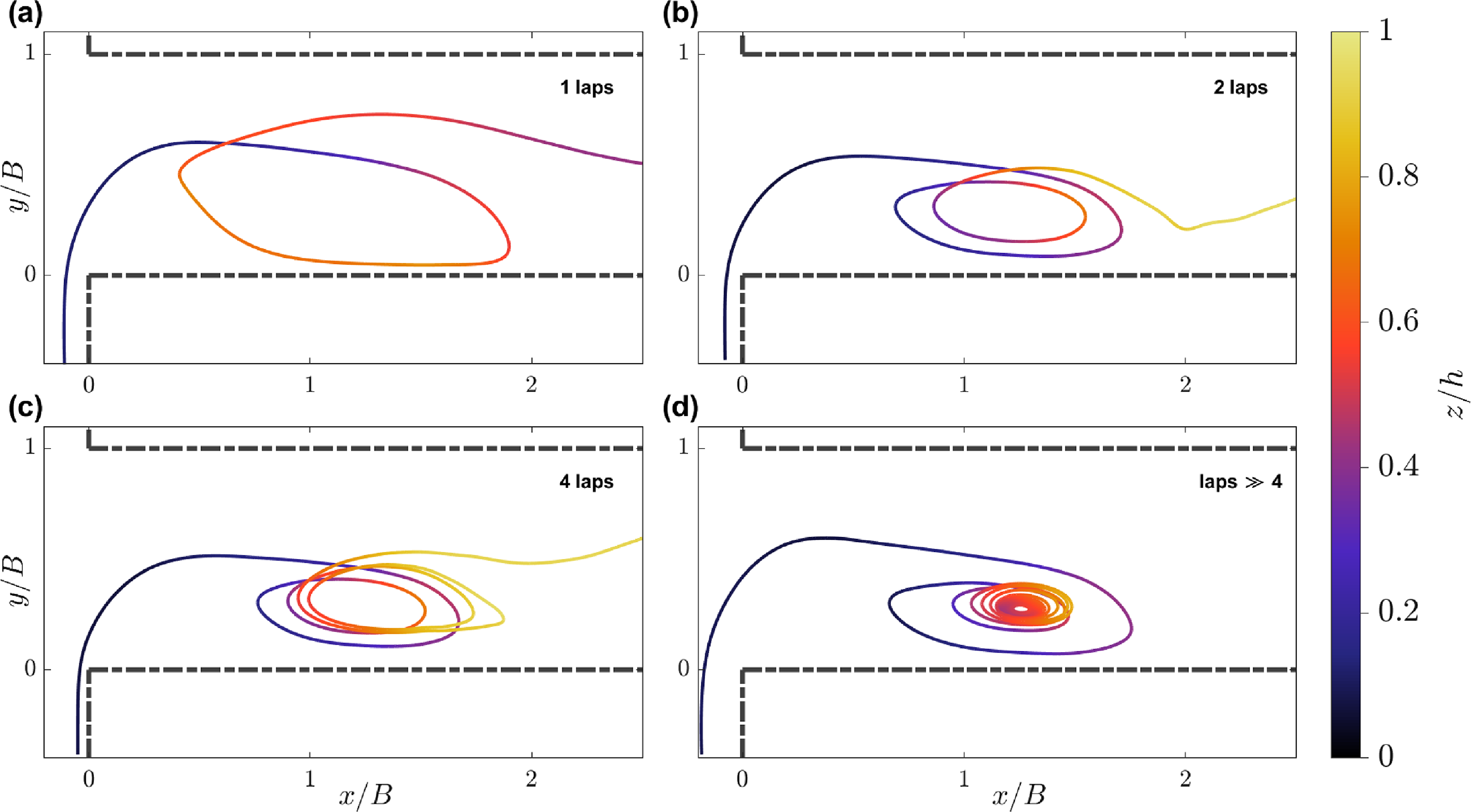
 x/B=0
 y/B=0
 z/h
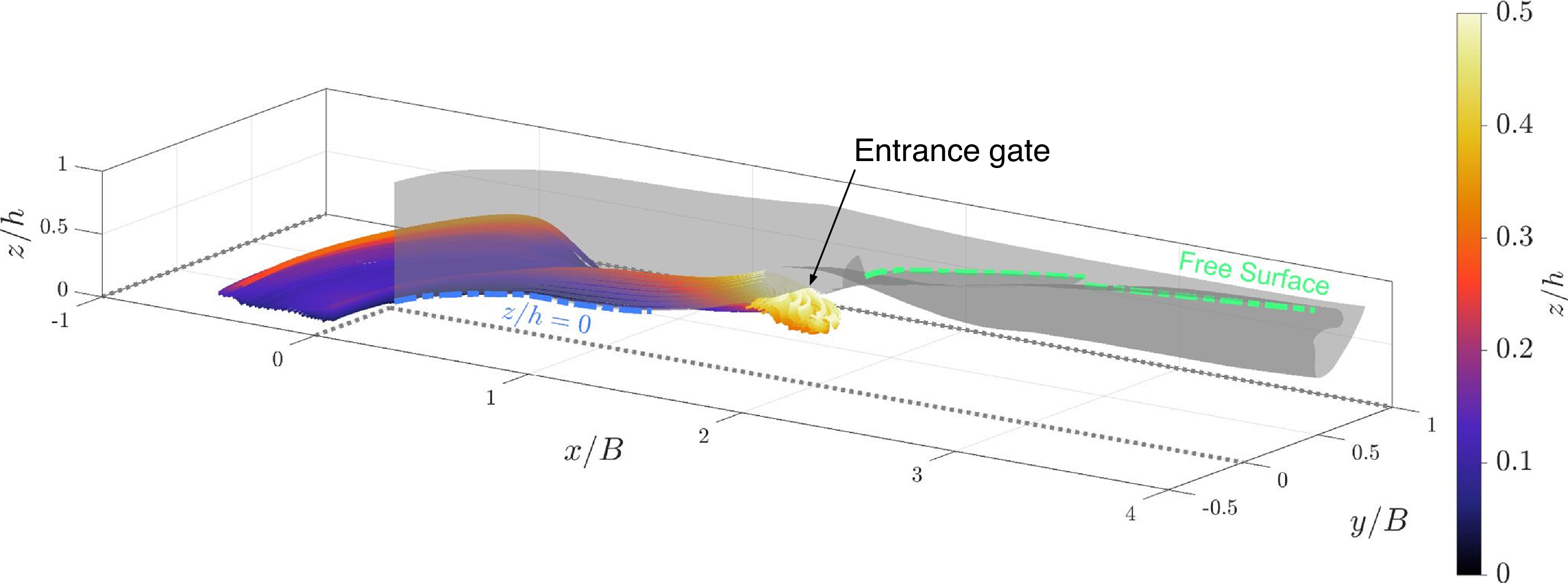
 Ux
 z/h
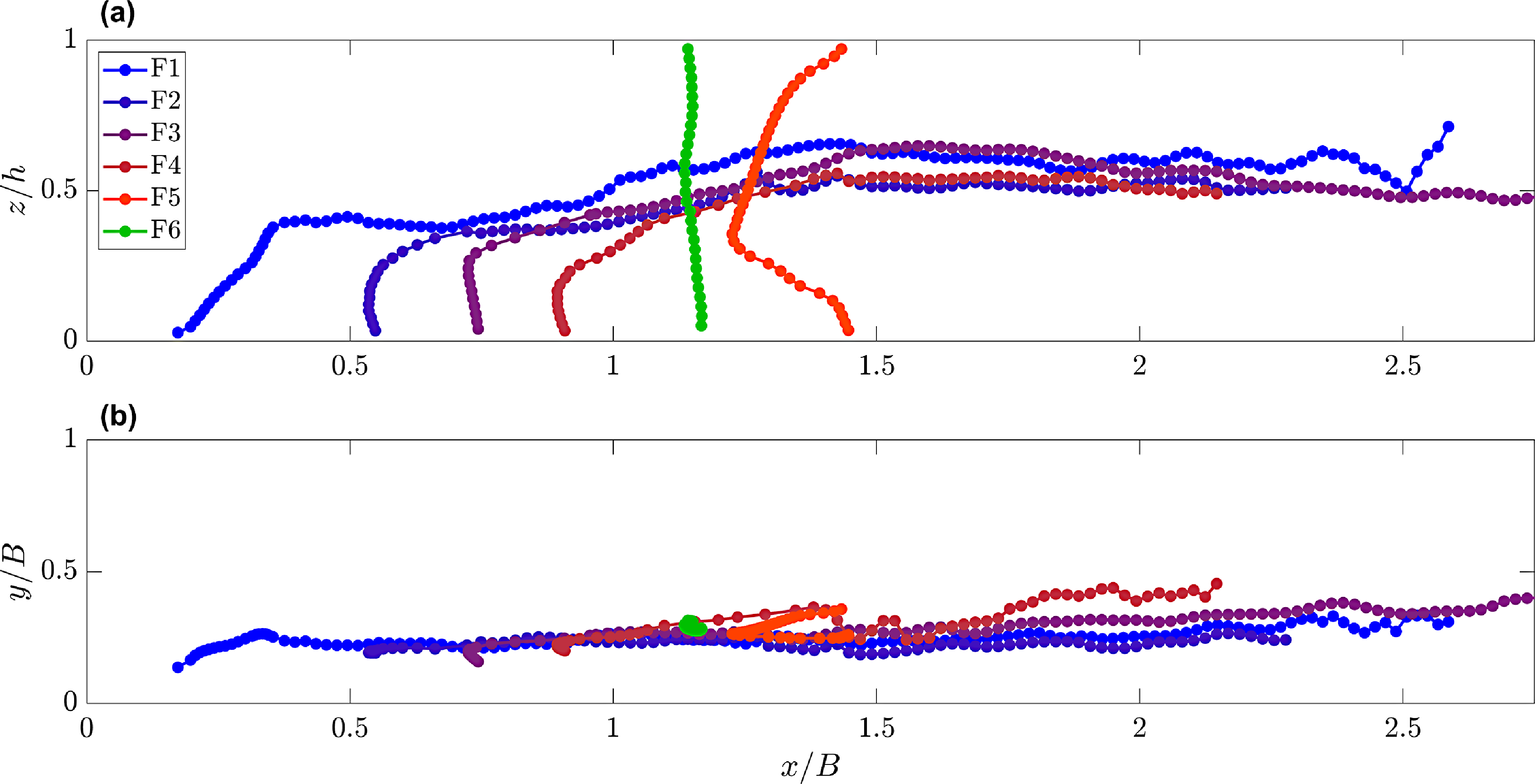
 Fr=0.215±0.05
 B/h
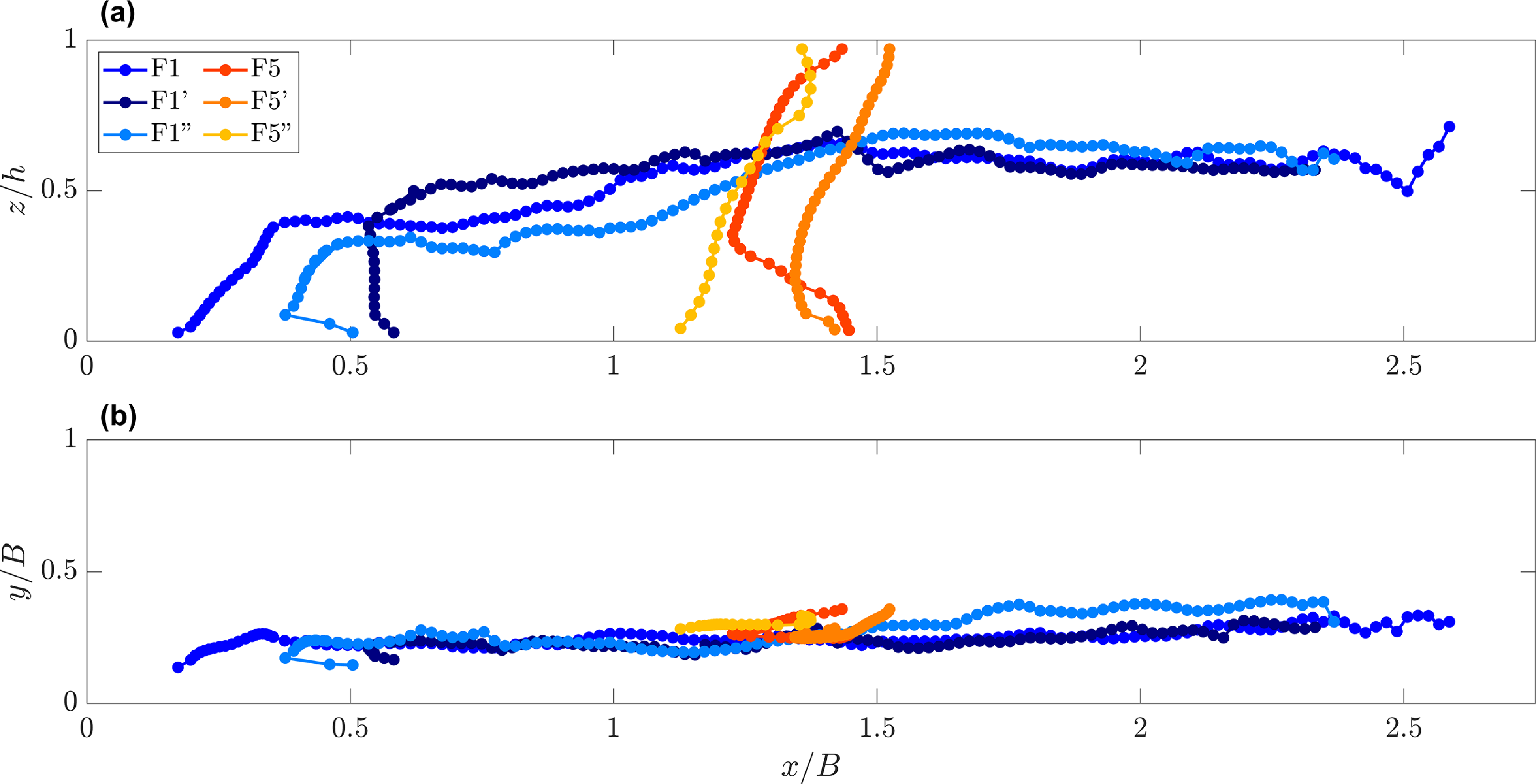
 B/h={2.95,4.17}
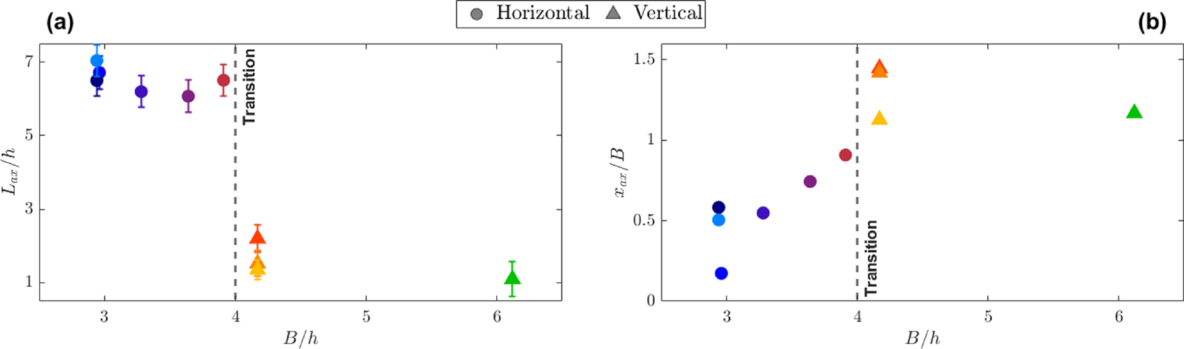
 Lax/h
 x/B=2.25
 B/h
 xax/B
 z/h=0
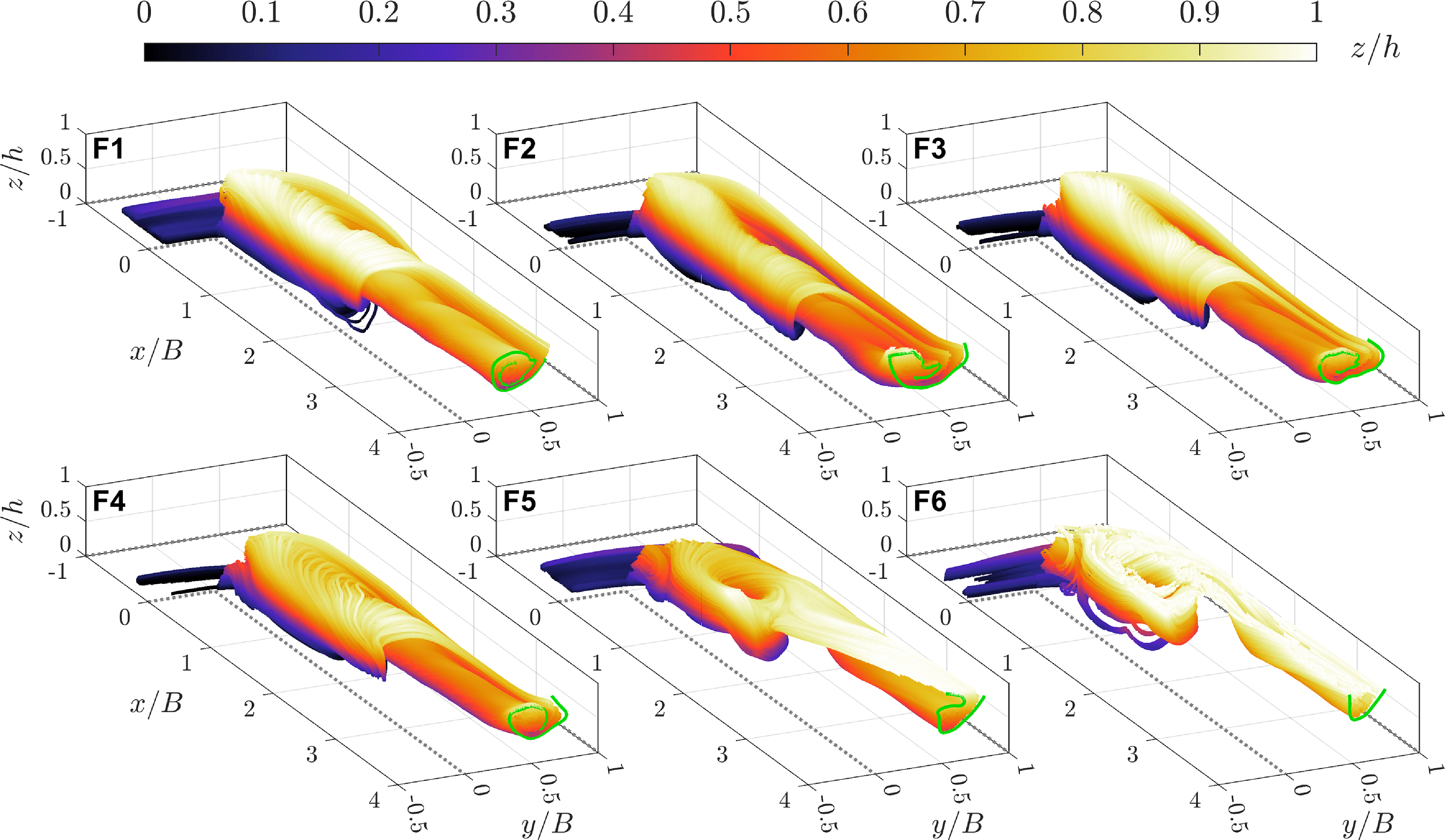
 z/h
 x/B=4
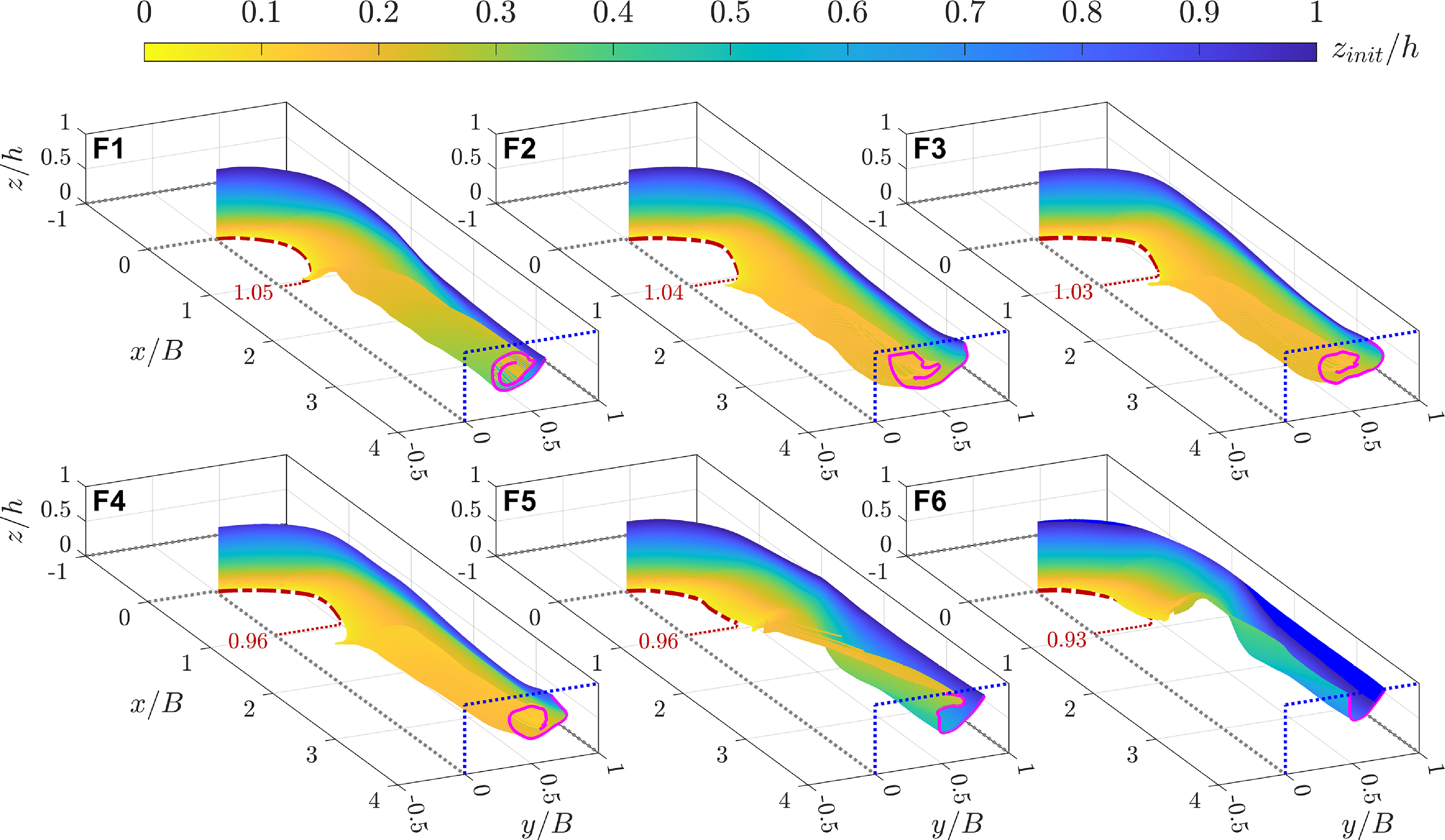
 zinit/h
 x/B=4
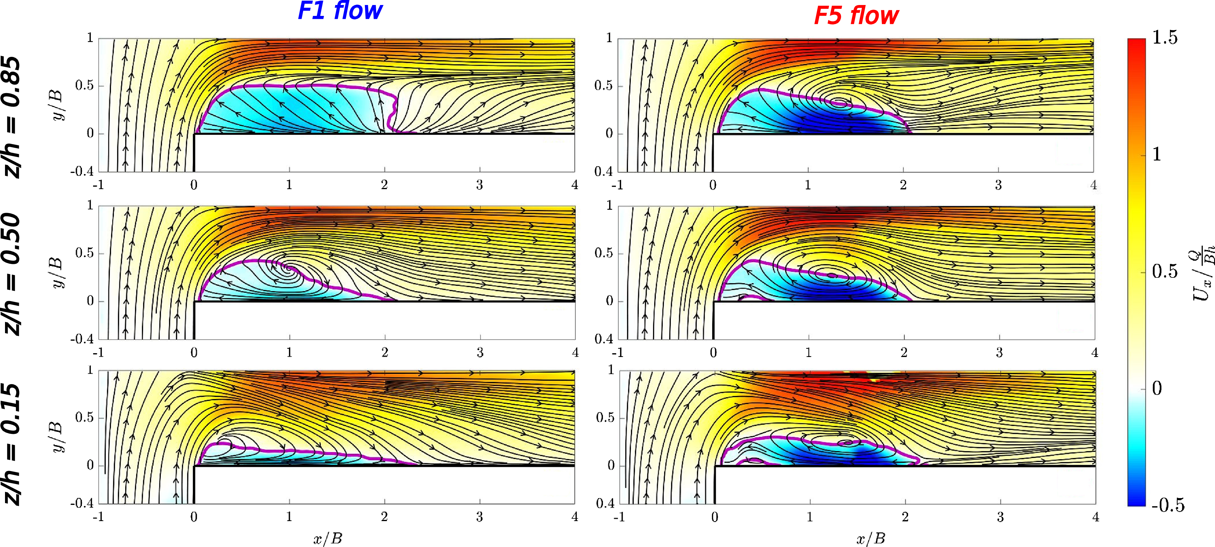
 z/h={0.15,0.50,0.85}
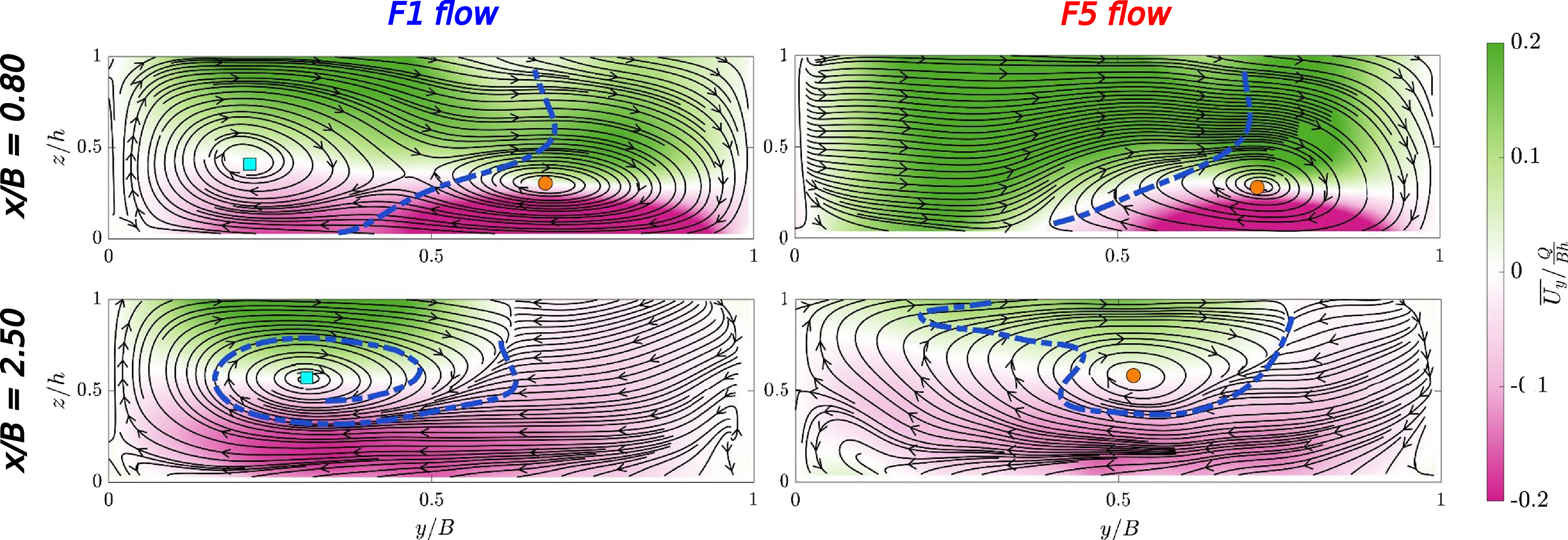
 x/B={0.80,2.50}
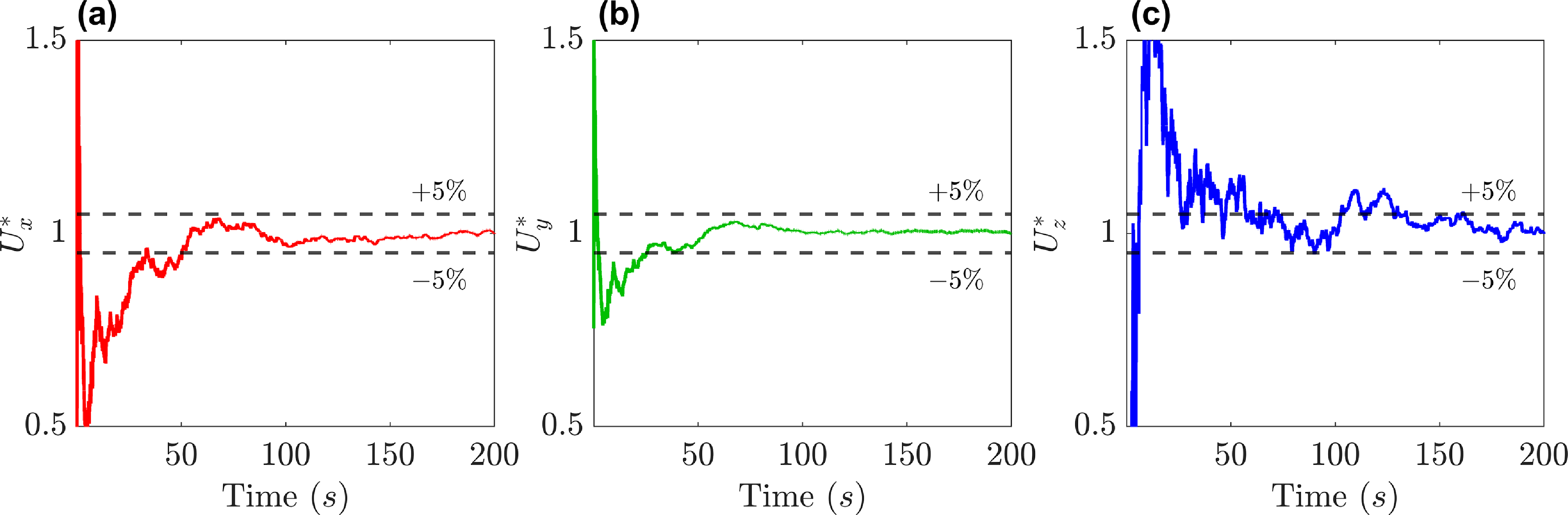
 Ux
 Uy
 Uz
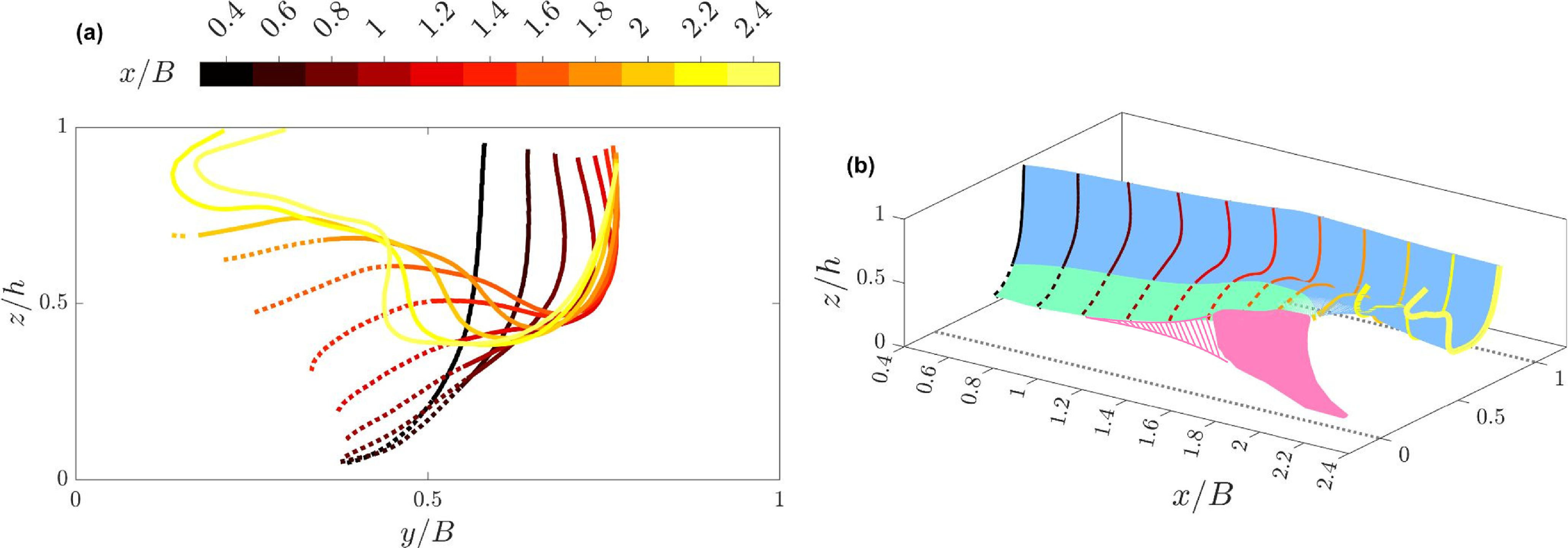
 x/B∈[0.4,2.4]
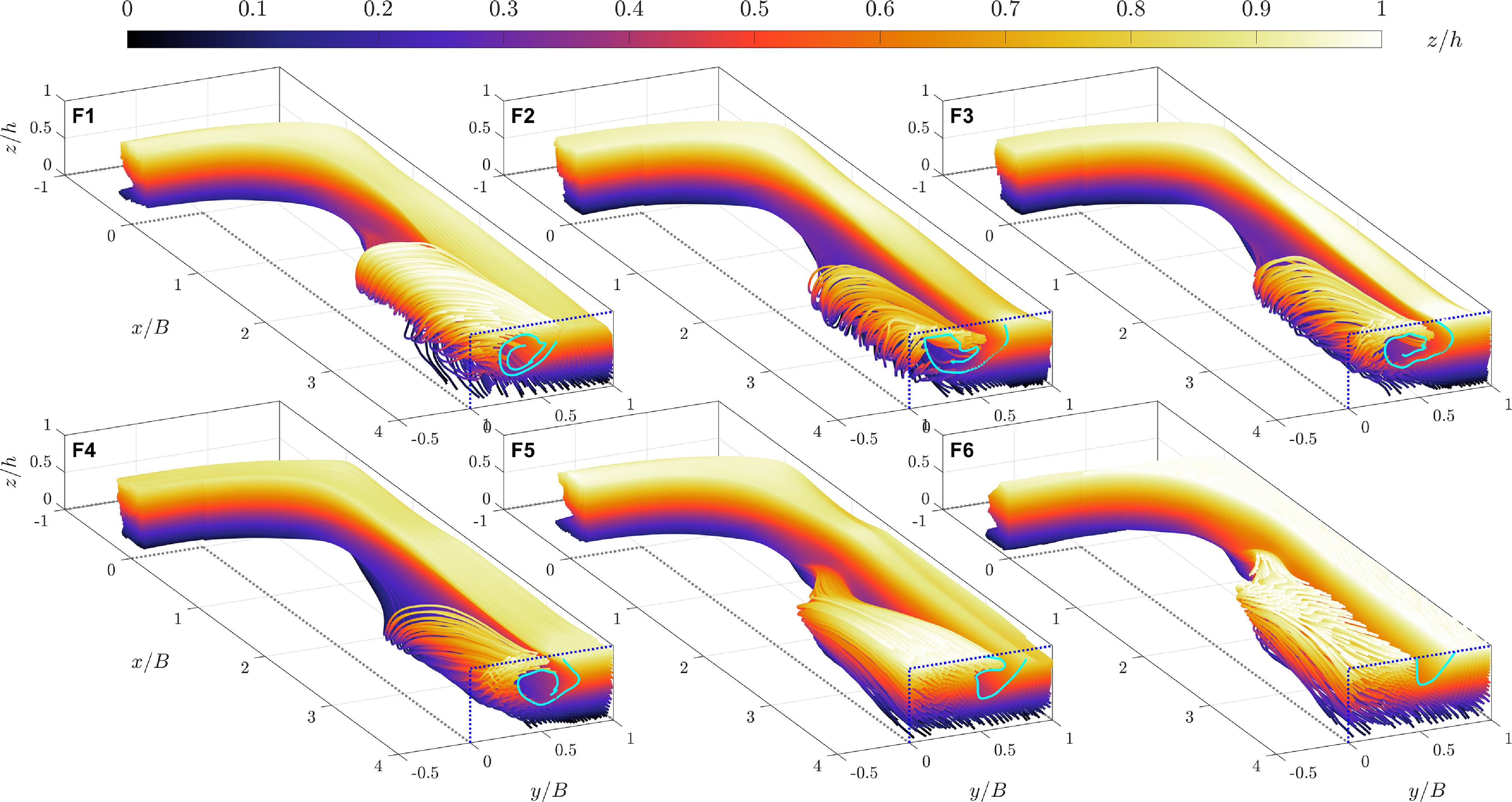
 z/h

 Open access

