1 Introduction
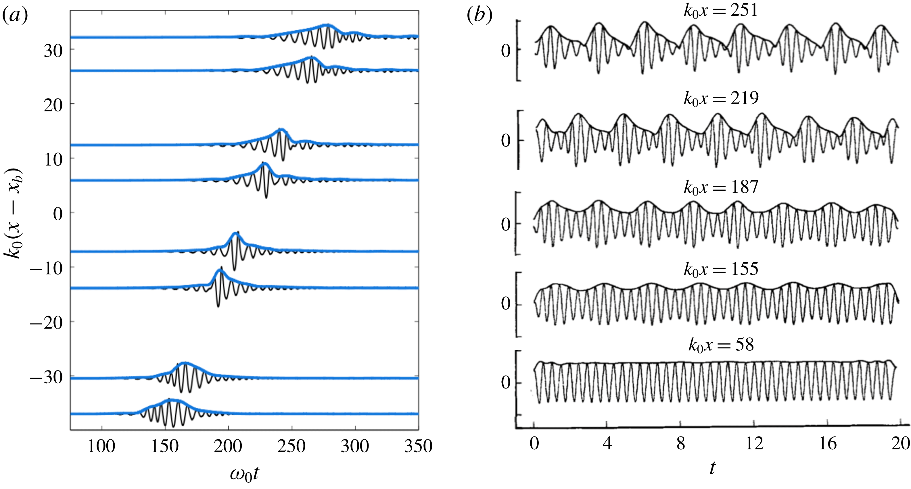
This investigation is concerned with initially narrow-banded and weakly nonlinear chirped compact deep-water wave groups and their evolution towards wave breaking. A distinguishing characteristic of these focusing packets is shown in figure 1, where packet asymmetry is manifest, and the packet slope reaches large negative values, resulting in wave breaking. The central question of this study is, which mechanisms control this behaviour in focusing nonlinear wave packets? To quantify this a dimensionless parameter,
 ${\mathcal{T}}={\mathcal{T}}(\unicode[STIX]{x1D716},\unicode[STIX]{x1D6E5})$
, for
 $\unicode[STIX]{x1D716}$
a measure of the linear prediction of the maximum wave slope at focusing and
 $\unicode[STIX]{x1D6E5}$
the dimensionless packet bandwidth, is proposed as a prediction of the local wave slope. When this parameter exceeds a certain threshold, wave breaking is expected.
Two laboratory examples of deep-water breaking waves. (a) Laboratory data from Drazen, Melville & Lenain (Reference Drazen, Melville and Lenain2008). A dispersive focusing technique is employed to create breaking around
 $k_{0}(x-x_{b})=0$
. The wave envelope is shown in blue, while the free surface displacement is given in black. Notice the strong asymmetry in the packet as breaking is approached. (b) The evolution of an initially uniform train of finite amplitude waves, from the laboratory experiments of Melville (Reference Melville1983). The initially uniform wave train experiences the Benjamin–Feir instability (Benjamin & Feir Reference Benjamin and Feir1967), leading to large modulations to the wave amplitude and phase, eventually leading to wave breaking around
 $k_{0}x=251$
.

Recently, physically motivated scaling arguments have been successful in describing bulk scale properties of the flow induced by deep-water wave breaking. For example, consider the energy dissipation rate due to deep-water breaking waves (Duncan Reference Duncan1981; Phillips Reference Phillips1985; Drazen et al.
Reference Drazen, Melville and Lenain2008; Romero, Melville & Kleiss Reference Romero, Melville and Kleiss2012; Sutherland & Melville Reference Sutherland and Melville2013; Deike, Popinet & Melville Reference Deike, Popinet and Melville2015). Drazen et al. (Reference Drazen, Melville and Lenain2008) found that the dissipation rate per unit length of length of breaking crest is given by
 $b_{0}(S-S_{0})^{5/2}\unicode[STIX]{x1D70C}c^{5}/g$
for
 $b_{0}$
a scaling constant,
 $S$
the linear prediction of the maximum wave slope at focusing,
 $\unicode[STIX]{x1D70C}$
the density of water,
 $c$
the phase velocity,
 $g$
the acceleration due to gravity and
 $S_{0}$
is the breaking threshold. Part of the motivation of this manuscript is to better understand this threshold quantity
 $S_{0}$
. For instance, does it depend on other quantities characterizing the wave packet such as the bandwidth? Improved understanding of the behaviour of this threshold may then be used to further constrain the scaling arguments that are used to close energy budgets between the atmosphere and ocean (Cavaleri, Fox-Kemper & Hemer Reference Cavaleri, Fox-Kemper and Hemer2012; Sutherland & Melville Reference Sutherland and Melville2015), and may be incorporated into wave models to parametrize the wave breaking statistics (Phillips Reference Phillips1985) in studies of air–sea interaction (Sullivan, McWilliams & Melville Reference Sullivan, McWilliams and Melville2007).
In this paper we employ the spatial modified nonlinear Schrödinger equation (hereinafter referred to as the MNLSE; Dysthe Reference Dysthe1979; Lo & Mei Reference Lo and Mei1985). The model is weakly nonlinear and narrow banded. How then may it be useful in describing wave breaking, which is a process that is very nonlinear (with the local free surface slope potentially going to negative infinity) and varies rapidly in space and time? Our approach is to distinguish physical mechanisms, and in particular bulk scale non-dimensional quantities describing these mechanisms, that characterize the magnitude of the gradients of the free surface displacement generated from initially narrow-banded weakly nonlinear wave packets. Here, using the variational method (Chandrasekhar Reference Chandrasekhar2013, §17) for an asymmetric trial function following Pizzo & Melville (Reference Pizzo and Melville2016, see also Anderson Reference Anderson1983), solutions for the packet amplitude, asymmetry, width and phase are found. A condition is derived, as a function of a non-dimensional number, under which the packet slope experiences large amplifications, implying its potential usefulness in quantifying the strength of packet focusing. Furthermore, the analysis hints at a quasi-self-similarity in the behaviour of the maximum slope in these focusing wave packets. Note, the mechanisms generating these large free surface displacement gradients are not directly responsible for wave breaking but may instead trigger higher-order local crest instabilities (e.g. the five wave resonance of steep waves (discussed in more detail below), see Longuet-Higgins Reference Longuet-Higgins1978; McLean et al. Reference McLean, Ma, Martin, Saffman and Yuen1981; Longuet-Higgins & Dommermuth Reference Longuet-Higgins and Dommermuth1997). Subsequently, this analysis is examined by integrating the fully nonlinear potential flow equations. Despite the limitations of the MNLSE (which have been elucidated in a number of laboratory and numerical experiments, see for instance Lo & Mei (Reference Lo and Mei1985), Shemer, Kit & Jiao (Reference Shemer, Kit and Jiao2002), Clamond et al. (Reference Clamond, Francius, Grue and Kharif2006)), due to the complexity of the full problem (Perlin, Choi & Tian Reference Perlin, Choi and Tian2013), there is insight gained by examining a minimal model that reproduces features that are observed in laboratory, numerical, and field observations of breaking waves.
Wave breaking in deep water may occur due to wave–wave interactions, wave–current interactions and wind–wave interactions (Melville Reference Melville1996). In this study, we are particularly interested in wave breaking due to wave–wave interactions so that we do not consider the effects of winds or external currents. Wave breaking has been studied theoretically since Stokes proposed the limiting form of permanent progressive waves (Stokes Reference Stokes1880, see also Craik Reference Craik2005). Mathematically, breaking is often identified with shock formation (Seliger Reference Seliger1968; Whitham Reference Whitham1974) or divergences in measures of the packet variance, as is common in virial theorem arguments for the nonlinear Schrödinger equation and its variants (Sulem & Sulem Reference Sulem and Sulem1999). For permanent progressive waves, five wave and higher resonances of very steep Stokes waves may rapidly lead to wave overturning (Longuet-Higgins & Dommermuth Reference Longuet-Higgins and Dommermuth1997), corresponding to a homoclinic bifurcation (Bridges Reference Bridges2004), but these waves tend to be of limited interest in practice due to their restriction to infinitesimal bandwidth. Although there has been significant theoretical and practical advances in our understanding of deep-water wave breaking, the principles guiding breaking are not fully known, making diagnostic and predictive modelling of a breaking threshold difficult (Perlin et al. Reference Perlin, Choi and Tian2013). Furthermore, it is not clear which variables describing the wave field are needed to characterize this behaviour.
Laboratory observations have been particularly successful in advancing our understanding of wave breaking. Two different generation mechanisms that lead to breaking are the evolution of an initially permanent progressive finite amplitude wave train to breaking (Melville Reference Melville1982, Reference Melville1983) and a dispersive focusing technique (Melville & Rapp Reference Melville and Rapp1985; Rapp & Melville Reference Rapp and Melville1990) originally proposed by Longuet-Higgins (Reference Longuet-Higgins1974). Breaking in both instances is shown in figure 1, where both amplitude amplification and a strong asymmetry in the packet envelope is evident.
Next, Dyachenko & Zakharov (Reference Dyachenko and Zakharov2011) derived an equation that is accurate to fourth order in wave slope, under the additional constraint that waves are travelling in one direction. Under these conditions, they derived a compact equation that is not limited by bandwidth constraints. Fedele (Reference Fedele2014) then used this equation to examine the evolution of an initially uniform very steep wave train (there the slope exceeds
 $0.577$
, while we recall the limiting Stokes wave has slope of around
 $0.443$
(Stokes Reference Stokes1880)), where the envelope amplitude and wavenumber evolution was hyperbolic, and derived a modified Camassa–Holm equation (Camassa & Holm Reference Camassa and Holm1993) governing the envelope evolution, which admits breaking. Dyachenko, Kachulin & Zakharov (Reference Dyachenko, Kachulin and Zakharov2017) also used this equation to examine steepening waves. However, breaking criterion and comparisons against the fully nonlinear potential flow equations were not provided, and it is not clear how accurate these descriptions are when applied so far outside of their asymptotic region of validity. Furthermore, the canonical transformations of the Zakharov equation needed to derive these equations (Dyachenko & Zakharov Reference Dyachenko and Zakharov2011) partially obscure the physics of these results.
Recently, Barthelemy et al. (Reference Barthelemy, Banner, Peirson, Fedele, Allis and Dias2018) proposed, and Saket et al. (Reference Saket, Peirson, Banner, Barthelemy and Allis2017, see also Khait & Shemer Reference Khait and Shemer2018) provided laboratory support for, a kinematic criterion for wave breaking (Perlin et al. Reference Perlin, Choi and Tian2013), providing a diagnostic tool to locally analyse the likelihood of breaking. The connection between this local kinematic behaviour and the initial conditions of dispersive focusing packets (which are characterized by linear predictions of their geometry at focusing) partially motivated this study. Note, power law behaviour of certain properties of breaking waves, such as length scales near breaking, have been examined theoretically in Pomeau et al. (Reference Pomeau, Le Berre, Guyenne and Grilli2008), but this study diagnoses the behaviour of the waves once breaking has taken place, and does not present a criterion nor a mechanism for breaking to occur.
The outline of this paper is as follows. In § 2, the modified nonlinear Schrödinger equation is reviewed. Next, in § 3, the evolution of initially narrow-banded weakly nonlinear chirped Gaussian packets is considered. A model is proposed to predict the maximum wave slope at focusing. The theory is then examined numerically in the fully nonlinear irrotational inviscid system in § 4. Finally, the results are discussed in § 5.
2 The modified nonlinear Schrödinger equation
In this section we review properties of the modified nonlinear Schrödinger equation (Dysthe Reference Dysthe1979), in a spatially mapped reference frame (Lo & Mei Reference Lo and Mei1985). This follows Pizzo & Melville (Reference Pizzo and Melville2016), and we note that a more general description of the Hamiltonian form of Dysthe’s equation may be found in Gramstad & Trulsen (Reference Gramstad and Trulsen2011, see also Kit & Shemer (Reference Kit and Shemer2002)).
2.1 Derivation of the MNLSE using Whitham’s method
The governing equation for irrotational inviscid two dimensional surface gravity waves is (see, for example, Phillips Reference Phillips1977)
 $$\begin{eqnarray}\unicode[STIX]{x1D6FB}^{\prime 2}\unicode[STIX]{x1D719}^{\prime }=0,\end{eqnarray}$$
together with boundary conditions
 $$\begin{eqnarray}\left.\unicode[STIX]{x1D719}_{t^{\prime }}^{\prime }+{\textstyle \frac{1}{2}}(\unicode[STIX]{x1D735}^{\prime }\unicode[STIX]{x1D719}^{\prime })^{2}+gz^{\prime }=0\right|_{z^{\prime }=\unicode[STIX]{x1D702}^{\prime }};\quad \left.\unicode[STIX]{x1D702}_{t^{\prime }}^{\prime }+\unicode[STIX]{x1D719}_{x^{\prime }}^{\prime }\unicode[STIX]{x1D702}_{x^{\prime }}^{\prime }=\unicode[STIX]{x1D719}_{z^{\prime }}^{\prime }\right|_{z^{\prime }=\unicode[STIX]{x1D702}^{\prime }},\end{eqnarray}$$
along with the condition of no flow at the bottom
 $\unicode[STIX]{x1D719}_{z^{\prime }}^{\prime }\rightarrow 0$
as
 $z^{\prime }\rightarrow -\infty$
, where
 $\unicode[STIX]{x1D719}^{\prime }$
is the velocity potential,
 $\unicode[STIX]{x1D702}^{\prime }$
is the free surface displacement,
 $\unicode[STIX]{x1D735}^{\prime }=(\unicode[STIX]{x2202}_{x^{\prime }},\unicode[STIX]{x2202}_{z^{\prime }})$
and
 $g$
is the acceleration due to gravity. Although the governing equation is linear, the boundary conditions are nonlinear, and more severely, are evaluated at a dependent variable of the system, namely
 $\unicode[STIX]{x1D702}^{\prime }$
.
In order to make analytic progress, asymptotic approximations are employed. The wave slope
 $\unicode[STIX]{x1D716}\equiv a_{0}k_{0}$
is a measure of the nonlinearity of the system, and is assumed to be much less than 1. Furthermore, if
 $\unicode[STIX]{x1D6FF}k$
is a perturbation to the characteristic wavenumber
 $k_{0}$
, then we define the bandwidth as
 $\unicode[STIX]{x1D6E5}\equiv |\unicode[STIX]{x1D6FF}k|/k_{0}$
. Now, unlike the canonical approach where
 $\unicode[STIX]{x1D6E5}\sim \unicode[STIX]{x1D716}$
, we instead leave the exact relationship between the two parameters general (see also the discussion in Phillips (Reference Phillips1981)). Finally, the characteristic angular frequency,
 $\unicode[STIX]{x1D714}_{0}$
, is related to the wavenumber by the linear dispersion relation for deep water surface gravity waves, i.e.
 $\unicode[STIX]{x1D714}_{0}^{2}=gk_{0}$
.
Following (Lo & Mei Reference Lo and Mei1985), we non-dimensionalize our system as follows:
 $$\begin{eqnarray}\displaystyle \left.\begin{array}{@{}c@{}}\unicode[STIX]{x1D719}=(a_{0}^{2}\unicode[STIX]{x1D714}_{0})^{-1}\unicode[STIX]{x1D719}^{\prime },\quad \unicode[STIX]{x1D702}=a_{0}^{-1}\unicode[STIX]{x1D702}^{\prime },\\ x=k_{0}x^{\prime },\quad t=\unicode[STIX]{x1D714}_{0}t^{\prime },\quad z=k_{0}z^{\prime }.\end{array}\right\} & & \displaystyle\end{eqnarray}$$
Expanding the velocity potential and free surface displacement as a series, we have (Chu & Mei Reference Chu and Mei1970)
 $$\begin{eqnarray}\displaystyle & \displaystyle \unicode[STIX]{x1D719}=\overline{\unicode[STIX]{x1D719}}(X,T;\unicode[STIX]{x1D716},\unicode[STIX]{x1D6E5})+\mathop{\sum }_{l=1}^{M}\mathop{\sum }_{m=1}^{M}\mathop{\sum }_{n\geqslant m}^{N}\unicode[STIX]{x1D716}^{n-1}\unicode[STIX]{x1D6E5}^{l-1}\unicode[STIX]{x1D719}_{lmn}(X,T,Z)\text{e}^{\text{i}m\unicode[STIX]{x1D703}}\text{e}^{mz}+\text{c.c.}, & \displaystyle\end{eqnarray}$$
 $$\begin{eqnarray}\displaystyle & \displaystyle \unicode[STIX]{x1D702}=\overline{\unicode[STIX]{x1D702}}(X,T;\unicode[STIX]{x1D716},\unicode[STIX]{x1D6E5})+\mathop{\sum }_{l=1}^{M}\mathop{\sum }_{m=1}^{M}\mathop{\sum }_{n\geqslant m}^{N}\unicode[STIX]{x1D716}^{n-1}\unicode[STIX]{x1D6E5}^{l-1}\unicode[STIX]{x1D702}_{lmn}(X,T)\text{e}^{\text{i}m\unicode[STIX]{x1D703}}+\text{c.c.}, & \displaystyle\end{eqnarray}$$
where
 $X=\unicode[STIX]{x0394}x,Z=\unicode[STIX]{x0394}z,T=\unicode[STIX]{x0394}t,\unicode[STIX]{x1D703}=x-t$
and
 $\text{c.c.}$
means complex conjugate;
 $\overline{\unicode[STIX]{x1D719}}$
and
 $\overline{\unicode[STIX]{x1D702}}$
are the mean (phase-averaged) velocity potential and free surface displacement, respectively, with their scale to be determined. Finally, we take the complex valued coefficient
 $\unicode[STIX]{x1D719}_{111}\equiv B$
as our dependent variable. This has important implications for the structure of the resulting governing equation (see the discussion in Kit & Shemer (Reference Kit and Shemer2002) and Trulsen (Reference Trulsen2006)).
The expansions of the dependent variables to third order in
 $\unicode[STIX]{x1D716}$
and second order in
 $\unicode[STIX]{x1D6E5}$
, appropriate for the MNLSE, are (Trulsen & Dysthe Reference Trulsen and Dysthe1997; Trulsen Reference Trulsen2006; Pizzo & Melville Reference Pizzo and Melville2016)
 $$\begin{eqnarray}\unicode[STIX]{x1D719}=\unicode[STIX]{x1D716}\overline{\unicode[STIX]{x1D719}}+\frac{1}{2}\left(\left[B-\text{i}\unicode[STIX]{x0394}zB_{X}-\frac{\unicode[STIX]{x1D6E5}^{2}}{2}z^{2}B_{XX}\right]\text{e}^{z}\text{e}^{\text{i}\unicode[STIX]{x1D703}}+\text{c.c.}\right),\end{eqnarray}$$
 $$\begin{eqnarray}\displaystyle \unicode[STIX]{x1D702} & = & \displaystyle \unicode[STIX]{x1D716}\unicode[STIX]{x1D6E5}\overline{\unicode[STIX]{x1D702}}+\frac{1}{2}\left(\left[\text{i}B+\frac{\unicode[STIX]{x1D6E5}}{2}B_{X}+\frac{\text{i}\unicode[STIX]{x1D6E5}^{2}}{8}B_{XX}+\frac{\text{i}\unicode[STIX]{x1D716}^{2}}{8}|B|^{2}B\right]\text{e}^{\text{i}\unicode[STIX]{x1D703}}\right.\nonumber\\ \displaystyle & & \displaystyle \left.+\,\left[-\frac{\unicode[STIX]{x1D716}}{2}B^{2}+\text{i}\unicode[STIX]{x1D716}\unicode[STIX]{x0394}BB_{X}\right]\text{e}^{2\text{i}\unicode[STIX]{x1D703}}+\frac{3\text{i}\unicode[STIX]{x1D716}^{2}}{8}B^{3}\text{e}^{3\text{i}\unicode[STIX]{x1D703}}+\text{c.c.}\right).\end{eqnarray}$$
Recall, equations (2.1), (2.2) can be reformulated in terms of a variational principle through the action (Luke Reference Luke1967; Zakharov Reference Zakharov1968; Miles Reference Miles1977)
 $$\begin{eqnarray}\int L\,\text{d}x\,\text{d}t=\int \left\{\unicode[STIX]{x1D716}\unicode[STIX]{x1D713}\unicode[STIX]{x1D702}_{t}-\unicode[STIX]{x1D716}\left(\int _{-\infty }^{\unicode[STIX]{x1D716}\unicode[STIX]{x1D702}}\frac{1}{2}(\unicode[STIX]{x1D6FB}\unicode[STIX]{x1D719})^{2}\,\text{d}z+\frac{1}{2}\unicode[STIX]{x1D702}^{2}\right)\right\}\,\text{d}x\,\text{d}t,\end{eqnarray}$$
where
 $\unicode[STIX]{x1D713}=\unicode[STIX]{x1D719}(x,z=\unicode[STIX]{x1D716}\unicode[STIX]{x1D702},t)$
is the velocity potential evaluated at the free surface.
Next, we substitute the form of the velocity potential and free surface displacement into (2.8). Furthermore, following Lo & Mei (Reference Lo and Mei1985), we map into a spatial reference frame by introducing the following transformation
 $$\begin{eqnarray}(2X-T)=\unicode[STIX]{x1D70F};\quad \unicode[STIX]{x0394}X=\unicode[STIX]{x1D712}.\end{eqnarray}$$
This reference frame is travelling at the linear group velocity, and for a fixed position
 $X$
,
 $\unicode[STIX]{x1D70F}$
is proportional to the negative of the elapsed time, while
 $\unicode[STIX]{x1D712}$
is related to the fetch (or stretched distance). Finally, for clarity of presentation we transform from the dependent variable
 $B$
to the dependent variable in the mapped frame
 $A$
.
Employing the mapping given by (2.9), the averaged Lagrangian (Whitham Reference Whitham1965, Reference Whitham1974), then becomes
 $$\begin{eqnarray}{\mathcal{L}}\equiv \frac{1}{2\unicode[STIX]{x03C0}}\int _{0}^{2\unicode[STIX]{x03C0}}L\,\text{d}\unicode[STIX]{x1D703}=\frac{\text{i}}{2}\left(A\frac{\unicode[STIX]{x2202}A^{\ast }}{\unicode[STIX]{x2202}\unicode[STIX]{x1D712}}-A^{\ast }\frac{\unicode[STIX]{x2202}A}{\unicode[STIX]{x2202}\unicode[STIX]{x1D712}}\right)-{\mathcal{H}},\end{eqnarray}$$
where
 ${\mathcal{H}}$
is defined as (cf. Gramstad & Trulsen Reference Gramstad and Trulsen2011, appendix C)
 $$\begin{eqnarray}{\mathcal{H}}=|A_{\unicode[STIX]{x1D70F}}|^{2}-\frac{\unicode[STIX]{x1D6FE}_{0}}{2}|A|^{4}-\frac{\unicode[STIX]{x1D6FC}_{0}}{2}|A|^{2}\mathbb{H}(|A|_{\unicode[STIX]{x1D70F}}^{2})+\text{i}\frac{\unicode[STIX]{x1D6FD}_{0}}{4}|A|^{2}(A^{\ast }A_{\unicode[STIX]{x1D70F}}-AA_{\unicode[STIX]{x1D70F}}^{\ast }),\end{eqnarray}$$
and
 $\unicode[STIX]{x1D6FE}_{0}=\unicode[STIX]{x1D716}^{2}/\unicode[STIX]{x1D6E5}^{2}$
,
 $\unicode[STIX]{x1D6FC}_{0}=2\unicode[STIX]{x1D716}^{2}/\unicode[STIX]{x1D6E5}$
,
 $\unicode[STIX]{x1D6FD}_{0}=8\unicode[STIX]{x1D716}^{2}/\unicode[STIX]{x1D6E5}$
, while
 $^{\ast }$
denotes the complex conjugate. Note,
 $\unicode[STIX]{x1D6FE}_{0}$
is a measure of the ratio of the
 $O(\unicode[STIX]{x1D716}^{2})$
nonlinearity to dispersion (this term has been shown to be important for statistical analogues of the NLSE (Alber Reference Alber1978; Onorato et al.
Reference Onorato, Osborne, Serio and Bertone2001; Janssen Reference Janssen2003) as well as the deterministic dynamics of the NLSE (Anderson Reference Anderson1983)) and the Hilbert transform
 $\mathbb{H}$
is defined as
 $$\begin{eqnarray}\mathbb{H}(|A|_{\unicode[STIX]{x1D70F}}^{2})=\frac{1}{\unicode[STIX]{x03C0}}P.V.\int _{-\infty }^{\infty }\frac{\unicode[STIX]{x2202}|A(\unicode[STIX]{x1D712},\unicode[STIX]{x1D70F}^{\prime })|^{2}}{\unicode[STIX]{x2202}\unicode[STIX]{x1D70F}^{\prime }}\frac{\text{d}\unicode[STIX]{x1D70F}^{\prime }}{\unicode[STIX]{x1D70F}-\unicode[STIX]{x1D70F}^{\prime }},\end{eqnarray}$$
with
 $P.V.$
meaning we are to take the principal value of the integral (Titchmarsh Reference Titchmarsh1948). Following Janssen (Reference Janssen1983, see also Akylas Reference Akylas1989) we have rewritten our action in terms of one variable by recognizing that
 $\overline{\unicode[STIX]{x1D711}_{\unicode[STIX]{x1D70F}}}$
and
 $\overline{\unicode[STIX]{x1D711}_{Z}}$
are harmonic conjugates, where
 $\unicode[STIX]{x1D711}$
is the velocity potential in this spatial reference frame. That is, these variables are real and imaginary parts of an analytic function in the lower half plane and hence we can connect the two variables, evaluated at
 $Z=0$
, via the Hilbert transform
 $\mathbb{H}$
.
As the linear dispersion is exactly represented in this spatial reference frame (Trulsen et al. Reference Trulsen, Kliakhandler, Dysthe and Velarde2000; Kit & Shemer Reference Kit and Shemer2002), only one term is needed to completely describe it. Besides making this equation more physically accurate, this also offers numerical advantages (Lo & Mei Reference Lo and Mei1985), and simplifies the equations algebraically.
The action associated with the Lagrangian density in the spatial reference frame, i.e. equation (2.10), is defined as
 $$\begin{eqnarray}{\mathcal{S}}(A,A^{\ast })=\int _{\unicode[STIX]{x1D712}_{0}}^{\unicode[STIX]{x1D712}_{f}}\int _{\mathbb{R}}{\mathcal{L}}\,\text{d}\unicode[STIX]{x1D70F}\,\text{d}\unicode[STIX]{x1D712},\end{eqnarray}$$
which is a functional over all admissible functions satisfying the prescribed conditions at
 $A(\unicode[STIX]{x1D70F},\unicode[STIX]{x1D712}_{0})$
and
 $A(\unicode[STIX]{x1D70F},\unicode[STIX]{x1D712}_{f})$
. Hamilton’s principle states that the governing equations of the system are found by requiring that
 ${\mathcal{S}}$
be stationary. That is, we seek solutions
 $(A,A^{\ast })$
such that
 $$\begin{eqnarray}\unicode[STIX]{x1D6FF}{\mathcal{S}}={\mathcal{S}}(A+\unicode[STIX]{x1D6FF}A,A^{\ast }+\unicode[STIX]{x1D6FF}A^{\ast })-{\mathcal{S}}(A,A^{\ast })=0,\end{eqnarray}$$
for infinitesimal
 $(\unicode[STIX]{x1D6FF}A,\unicode[STIX]{x1D6FF}A^{\ast })$
. Substituting the Lagrangian density into the action, then applying Hamilton’s principle, and recalling the anti-self-adjoint nature of the Hilbert transform (Titchmarsh Reference Titchmarsh1948), gives us (Lo & Mei Reference Lo and Mei1985; Kit & Shemer Reference Kit and Shemer2002)
 $$\begin{eqnarray}\frac{\unicode[STIX]{x2202}A}{\unicode[STIX]{x2202}\unicode[STIX]{x1D712}}+\text{i}\frac{\unicode[STIX]{x2202}^{2}A}{\unicode[STIX]{x2202}\unicode[STIX]{x1D70F}^{2}}+\text{i}\unicode[STIX]{x1D6FE}_{0}|A|^{2}A+\text{i}\unicode[STIX]{x1D6FC}_{0}A\mathbb{H}\left(\frac{\unicode[STIX]{x2202}|A|^{2}}{\unicode[STIX]{x2202}\unicode[STIX]{x1D70F}}\right)+\unicode[STIX]{x1D6FD}_{0}|A|^{2}\frac{\unicode[STIX]{x2202}A}{\unicode[STIX]{x2202}\unicode[STIX]{x1D70F}}=0.\end{eqnarray}$$
The constants
 $(\unicode[STIX]{x1D6FC}_{0},\unicode[STIX]{x1D6FD}_{0})$
also make it easy to track the induced mean flow (which is related to the term with coefficient
 $\unicode[STIX]{x1D6FC}_{0}$
), and the asymmetric self-steepening term (which is related to the term with coefficient
 $\unicode[STIX]{x1D6FD}_{0}$
) in the ensuing calculations. Note, for
 $\unicode[STIX]{x1D6E5}=\unicode[STIX]{x1D716}$
, we return the standard form of the MNLSE.
This equation is usually written as a set of coupled partial differential equations (PDEs) in two dependent variables,
 $(A,\overline{\unicode[STIX]{x1D711}}|_{Z=0})$
. The two variables are connected by the relation
 $$\begin{eqnarray}\left.\frac{\unicode[STIX]{x2202}\overline{\unicode[STIX]{x1D711}}}{\unicode[STIX]{x2202}Z}\right|_{Z=0}=\frac{\unicode[STIX]{x2202}|A|^{2}}{\unicode[STIX]{x2202}\unicode[STIX]{x1D70F}},\end{eqnarray}$$
which implies that gradients in the radiation stress lead to the generation of a mean flow (Longuet-Higgins & Stewart Reference Longuet-Higgins and Stewart1964; Dysthe Reference Dysthe1979; McIntyre Reference McIntyre1981).
2.2 Conservation laws
A benefit of the above use of Whitham’s method is that symmetries of the action (2.13) may be connected with conservation laws using Noether’s theorem. In particular, Pizzo & Melville (Reference Pizzo and Melville2016) were able to identify several symmetries of the action of the Lagrangian associated with (2.15). They found that (2.15) conserves wave action,
 $$\begin{eqnarray}\frac{\unicode[STIX]{x2202}|A|^{2}}{\unicode[STIX]{x2202}\unicode[STIX]{x1D712}}+\frac{\unicode[STIX]{x2202}}{\unicode[STIX]{x2202}\unicode[STIX]{x1D70F}}\left(\text{i}(A^{\ast }A_{\unicode[STIX]{x1D70F}}-AA_{\unicode[STIX]{x1D70F}}^{\ast })+\frac{\unicode[STIX]{x1D6FD}_{0}}{2}|A|^{4}\right)=0,\end{eqnarray}$$
as well as the wave action weighted frequency (Trulsen & Dysthe Reference Trulsen and Dysthe1997)
 $$\begin{eqnarray}\frac{\unicode[STIX]{x2202}}{\unicode[STIX]{x2202}\unicode[STIX]{x1D712}}(\text{i}(A^{\ast }A_{\unicode[STIX]{x1D70F}}-AA_{\unicode[STIX]{x1D70F}}^{\ast }))+\frac{\unicode[STIX]{x2202}{\mathcal{G}}}{\unicode[STIX]{x2202}\unicode[STIX]{x1D70F}}+2\unicode[STIX]{x1D6FC}_{0}|A|_{\unicode[STIX]{x1D70F}}^{2}\mathbb{H}(|A|_{\unicode[STIX]{x1D70F}}^{2})=0,\end{eqnarray}$$
where
 $$\begin{eqnarray}{\mathcal{G}}=2|A_{\unicode[STIX]{x1D70F}}|^{2}-(AA_{\unicode[STIX]{x1D70F}\unicode[STIX]{x1D70F}}^{\ast }-A^{\ast }A_{\unicode[STIX]{x1D70F}\unicode[STIX]{x1D70F}})-\unicode[STIX]{x1D6FE}_{0}|A|^{4}+\text{i}\unicode[STIX]{x1D6FD}_{0}|A|^{2}(A^{\ast }A_{\unicode[STIX]{x1D70F}}-AA_{\unicode[STIX]{x1D70F}}^{\ast })-2\unicode[STIX]{x1D6FC}_{0}|A|^{2}\mathbb{H}(|A|_{\unicode[STIX]{x1D70F}}^{2}).\end{eqnarray}$$
As was noted in Pizzo & Melville (Reference Pizzo and Melville2016), equation (2.18) does not take the form of a local conservation law due to the last term in (2.18), which cannot be written as a perfect derivative. However, the integral quantity
 $\int \text{i}(A^{\ast }A_{\unicode[STIX]{x1D70F}}-AA_{\unicode[STIX]{x1D70F}}^{\ast })\,\text{d}\unicode[STIX]{x1D70F}$
is still conserved, as the final term on the left-hand side of (2.18) integrates to zero due to the anti-self-adjoint nature of the Hilbert transform (Titchmarsh Reference Titchmarsh1948).
3 Focusing wave packets
The goal of this section is to identify non-dimensional parameters that characterize wave focusing as governed by (2.15). In the absence of a canonical structure to analyse for focusing wave packets, we must come up with a rational way to analytically examine the evolution of this system. To this end, following work in fluid mechanics (Chandrasekhar Reference Chandrasekhar2013) and optics (Agrawal Reference Agrawal2007), ansätze are made for a trial function and a variational method is used to determine its evolution.
Theoretically, we consider chirped, initially narrow-banded and weakly nonlinear, Gaussian wave packets. These waves are similar to the dispersive focusing wave packets originally proposed by Longuet-Higgins (Reference Longuet-Higgins1974) and used extensively in laboratory experiments on breaking waves (Melville & Rapp Reference Melville and Rapp1985; Rapp & Melville Reference Rapp and Melville1990; Tian, Perlin & Choi Reference Tian, Perlin and Choi2010; Perlin et al. Reference Perlin, Choi and Tian2013). Longer (faster) waves are generated after shorter (slower) waves, leading to energy focusing in a region of space and time, possibly leading to breaking.
Chirped Gaussian wave packets satisfying the linear Schrödinger (i.e.
 $\unicode[STIX]{x1D6FE}_{0}=\unicode[STIX]{x1D6FC}_{0}=\unicode[STIX]{x1D6FD}_{0}=0$
) take the form
 $$\begin{eqnarray}A=\frac{h_{0}}{\sqrt{1-2\text{i}\unicode[STIX]{x1D6EC}\unicode[STIX]{x1D712}}}\text{e}^{-\unicode[STIX]{x1D6EC}\unicode[STIX]{x1D70F}^{2}/2(1-2\text{i}\unicode[STIX]{x1D6EC}\unicode[STIX]{x1D712})},\end{eqnarray}$$
where
 $\unicode[STIX]{x1D6EC}=(1+\text{i}C)w^{-2}$
, for
 $C$
the packet chirp, and
 $w$
the packet width. The packet bandwidth then scales with
 $w|\unicode[STIX]{x1D6EC}|=\sqrt{1+C^{2}}w^{-1}$
(Agrawal Reference Agrawal2007).
3.1 Variational equations
Following Pizzo & Melville (Reference Pizzo and Melville2016), we use the variational method (Anderson Reference Anderson1983; Agrawal Reference Agrawal2007; Chandrasekhar Reference Chandrasekhar2013), to derive approximate analytic forms for the evolution of physically important packet parameters. This qualifies and quantifies the packet evolution, and forms a useful tool to understand the bulk scale properties of the wave envelope during focusing. The success of this approach relies on a trial function which captures the essence of the phenomenon in question, without being too algebraically complicated.
To this end, we recall that in the absence of linear dispersion, as was discussed by Pizzo & Melville (Reference Pizzo and Melville2016), equations (2.17) and (2.18) decouple, and may be solved using the method of characteristics. For small
 $\unicode[STIX]{x1D6FD}_{0}\unicode[STIX]{x1D70C}^{2}\unicode[STIX]{x1D712}$
, solutions to the wave action equation (i.e. (2.17)) takes the form
 $$\begin{eqnarray}\unicode[STIX]{x1D70C}\approx \unicode[STIX]{x1D70C}_{0}+\unicode[STIX]{x1D6FD}_{0}\unicode[STIX]{x1D70C}_{0}^{2}\unicode[STIX]{x1D70C}_{0}^{\prime }\unicode[STIX]{x1D712},\end{eqnarray}$$
where the subscript
 $0$
means we are evaluating these functions at
 $\unicode[STIX]{x1D712}=0$
.
This implies that that for an initially chirped Gaussian wave packet, we should try a trial function of the form (Anderson Reference Anderson1983)
 $$\begin{eqnarray}{\mathcal{A}}=(a(\unicode[STIX]{x1D712})\text{e}^{-\unicode[STIX]{x1D70F}^{2}/2w(\unicode[STIX]{x1D712})^{2}}+\unicode[STIX]{x1D6FD}_{0}s(\unicode[STIX]{x1D712})\unicode[STIX]{x1D70F}\text{e}^{-3\unicode[STIX]{x1D70F}^{2}/2w(\unicode[STIX]{x1D712})^{2}})\text{e}^{\text{i}(C(\unicode[STIX]{x1D712})\unicode[STIX]{x1D70F}^{2}/2+G(\unicode[STIX]{x1D712})+\unicode[STIX]{x1D6FD}_{0}F(\unicode[STIX]{x1D712})\unicode[STIX]{x1D70F})},\end{eqnarray}$$
where we are solving for the six real functions
 $(a,s,w,C,F,G)$
, governing the amplitude of the symmetric component of the packet
 $a$
, the asymmetric amplitude
 $s$
, the packet width
 $w$
, the chirp
 $C$
, the mean frequency
 $F$
and the phase shift
 $G$
.
To employ the variational technique we then substitute our trial wave function into the action, i.e. (2.13), so that to the same order of approximation as (2.15), we find
 $$\begin{eqnarray}\displaystyle \mathfrak{L} & = & \displaystyle \int _{-\infty }^{\infty }L\,\text{d}\unicode[STIX]{x1D70F}=\sqrt{\frac{2}{\unicode[STIX]{x03C0}}}\unicode[STIX]{x1D6FC}_{0}\unicode[STIX]{x1D718}_{0}a^{4}-\sqrt{2}\frac{a^{2}}{w}+\unicode[STIX]{x1D6FE}_{0}a^{4}w\end{eqnarray}$$
 $$\begin{eqnarray}\displaystyle & & \displaystyle -\,\sqrt{2}a^{2}C^{2}w^{3}+\frac{a^{2}w^{3}C^{\prime }}{\sqrt{2}}+2\sqrt{2}a^{2}wG^{\prime },\end{eqnarray}$$
where
 $\unicode[STIX]{x1D718}_{0}$
is a constant given by
 $$\begin{eqnarray}\unicode[STIX]{x1D718}_{0}=\int _{-\infty }^{\infty }\text{e}^{-(\unicode[STIX]{x1D70F}/w)^{2}}\mathbb{H}((\text{e}^{-(\unicode[STIX]{x1D70F}/w)^{2}})_{\unicode[STIX]{x1D70F}})\,\text{d}\unicode[STIX]{x1D70F}=1,\end{eqnarray}$$
as the Hilbert transform of the Gaussian function may be written in terms of the Dawson function (Temme Reference Temme2010), so that this integral may be computed analytically.
We begin by noting that the integral form of conservation of wave action, i.e. equation (2.17), becomes
 $$\begin{eqnarray}E_{0}=\int _{-\infty }^{\infty }|A|^{2}\,\text{d}\unicode[STIX]{x1D70F}=\sqrt{\unicode[STIX]{x03C0}}a^{2}w+O(\unicode[STIX]{x1D6FD}_{0}^{2}),\end{eqnarray}$$
where
 $E_{0}$
is a specified constant (independent of the scales
 $\unicode[STIX]{x1D716}$
and
 $\unicode[STIX]{x1D6E5}$
) based on the initial wave form. Furthermore, conservation of mean frequency, i.e. the integral of (2.18), gives
 $$\begin{eqnarray}P_{0}=\frac{\text{i}}{E_{0}}\int _{-\infty }^{\infty }(A^{\ast }A_{\unicode[STIX]{x1D70F}}-AA_{\unicode[STIX]{x1D70F}}^{\ast })\,\text{d}\unicode[STIX]{x1D70F}=\frac{aw\unicode[STIX]{x1D6FD}_{0}}{8}\left(aF+\frac{Csw^{2}}{2\sqrt{2}}\right),\end{eqnarray}$$
which for the initially chirped Gaussian function (3.1) must be taken to be zero, so that
 $$\begin{eqnarray}F=-\frac{1}{2\sqrt{2}}\frac{sw^{5/2}C}{E_{0}^{1/2}}.\end{eqnarray}$$
We can now apply Hamilton’s principle to each of the dependent variables, yielding a set of coupled ordinary differential equations. Taking variations with respect to
 $w$
implies
 $$\begin{eqnarray}G^{\prime }+\frac{3}{4}w^{2}C^{\prime }-\frac{3}{2}C^{2}w^{2}+\frac{1}{2w^{2}}+\frac{\unicode[STIX]{x1D6FE}_{0}a^{2}}{2\sqrt{2}}=0,\end{eqnarray}$$
while variations with respect to
 $G$
gives
 $$\begin{eqnarray}(a^{2}w)^{\prime }=0,\end{eqnarray}$$
which is consistent with equation (3.7).
Next, varying
 $\mathfrak{L}$
with respect to
 $a$
we find
 $$\begin{eqnarray}G^{\prime }+\frac{1}{4}w^{2}C^{\prime }-\frac{1}{2}C^{2}w^{2}+\frac{\unicode[STIX]{x1D6FC}_{0}a^{2}}{\sqrt{\unicode[STIX]{x03C0}}w}-\frac{1}{2w^{2}}+\unicode[STIX]{x1D6FE}_{0}\frac{a^{2}}{\sqrt{2}}=0,\end{eqnarray}$$
while variations with respect to
 $C$
yields
 $$\begin{eqnarray}4a^{2}w^{3}C+(a^{2}w^{3})^{\prime }=0.\end{eqnarray}$$
Next, recall Pizzo & Melville (Reference Pizzo and Melville2016) found that the centroid of packets governed by the MNLSE, in the frame of reference moving at the linear group velocity, have a finite amplitude correction analogous to the Stokes correction for permanent progressive waves. There, it was found that (for
 $P_{0}=0$
)
 $$\begin{eqnarray}\frac{\text{d}}{\text{d}\unicode[STIX]{x1D712}}\frac{1}{E_{0}}\int _{-\infty }^{\infty }\unicode[STIX]{x1D70F}|A|^{2}\,\text{d}\unicode[STIX]{x1D70F}=\frac{\unicode[STIX]{x1D6FD}_{0}}{2E_{0}}\int _{-\infty }^{\infty }|A|^{4}\,\text{d}\unicode[STIX]{x1D70F}.\end{eqnarray}$$
Substituting our trial function into this equation, we find a relationship for
 $s$
,
 $$\begin{eqnarray}s^{\prime }+\frac{5}{2}\frac{w^{\prime }}{w}s=\frac{8E_{0}^{3/2}}{w^{7/2}}.\end{eqnarray}$$
Next, from equation (3.7), equation (3.13) can be rewritten to find
 $$\begin{eqnarray}C=-\frac{1}{2}\frac{w^{\prime }}{w}=-\frac{1}{2}\frac{\text{d}\ln w}{\text{d}\unicode[STIX]{x1D712}}.\end{eqnarray}$$
Then, subtracting (3.10) from (3.12) and substituting in (3.16), we have
 $$\begin{eqnarray}w^{\prime \prime }+\unicode[STIX]{x1D6FE}_{0}E_{0}\sqrt{\frac{2}{\unicode[STIX]{x03C0}}}\frac{1}{w^{2}}+4\left(-1+\frac{\unicode[STIX]{x1D6FC}_{0}E_{0}}{\unicode[STIX]{x03C0}}\right)\frac{1}{w^{3}}=0.\end{eqnarray}$$
Multiplying by
 $w^{\prime }$
and integrating once, we find an equation describing a particle trapped in a potential well,
 $$\begin{eqnarray}\frac{1}{2}\left(\frac{\text{d}w}{\text{d}\unicode[STIX]{x1D712}}\right)^{2}+\unicode[STIX]{x1D6F1}(w)=0,\end{eqnarray}$$
where the potential
 $\unicode[STIX]{x1D6F1}(w)$
is given by
 $$\begin{eqnarray}\unicode[STIX]{x1D6F1}(w)=2\left(1-\frac{\unicode[STIX]{x1D6FC}_{0}E_{0}}{\unicode[STIX]{x03C0}}\right)\frac{1}{w^{2}}-\sqrt{\frac{2}{\unicode[STIX]{x03C0}}}\frac{\unicode[STIX]{x1D6FE}_{0}E_{0}}{w}+\unicode[STIX]{x1D6F1}_{0},\end{eqnarray}$$
and
 $\unicode[STIX]{x1D6F1}_{0}$
is an integration constant chosen to satisfy the initial conditions, that is
 $$\begin{eqnarray}\unicode[STIX]{x1D6F1}_{0}=-1/2w_{0}^{^{\prime }2}-2\left(1-\frac{\unicode[STIX]{x1D6FC}_{0}E_{0}}{\unicode[STIX]{x03C0}}\right)\frac{1}{w_{0}^{2}}+\sqrt{\frac{2}{\unicode[STIX]{x03C0}}}\frac{\unicode[STIX]{x1D6FE}_{0}E_{0}}{w_{0}}.\end{eqnarray}$$
The initial velocity of the particle in the well is set by the chirp of the packet and the initial width, as is evident by (3.16). Equation (3.19) makes it clear that the dynamics of
 $w$
is set by the size of
 $(\unicode[STIX]{x1D716}/\unicode[STIX]{x1D6E5})^{2}$
and
 $\unicode[STIX]{x1D716}^{2}/\unicode[STIX]{x1D6E5}$
. Note, throughout the rest of this discussion we take
 $E_{0}$
to be
 $\sqrt{\unicode[STIX]{x03C0}}$
, so that
 $a_{0}^{2}w_{0}=1$
.
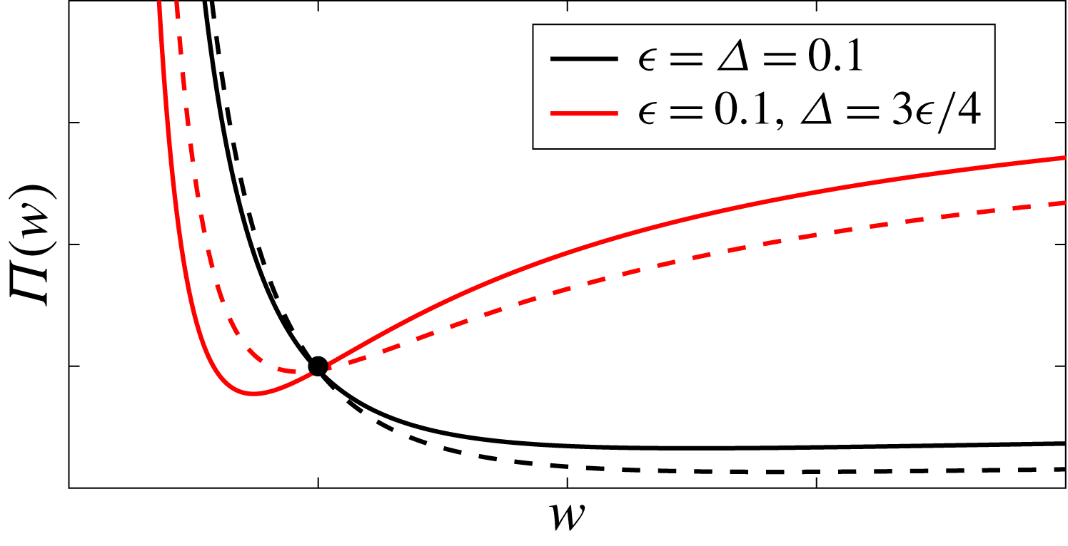
Examples of potentials for two values of
 $\unicode[STIX]{x1D716}^{2}/\unicode[STIX]{x1D6E5}$
are shown in figure 2. There, the black dot represents the initial packet width (taken to be
 $w_{0}=1$
). We take
 $C_{0}<0$
so that the packet width
 $w$
decreases, leading to focusing. For increasing values of
 $\unicode[STIX]{x1D716}^{2}/\unicode[STIX]{x1D6E5}$
, this focusing event becomes more pronounced as linear dispersion is retarded by the induced mean flow.
The packet width may be solved for implicitly, as we may rewrite (3.18) as
 $$\begin{eqnarray}\sqrt{2}\unicode[STIX]{x1D712}=\int _{1}^{w}\frac{\tilde{w}\text{d}\tilde{w}}{\sqrt{-\tilde{w}^{2}\unicode[STIX]{x1D6F1}_{0}+\sqrt{2}\unicode[STIX]{x1D6FE}_{0}\tilde{w}-2(1-\unicode[STIX]{x1D6FC}_{0}/\sqrt{\unicode[STIX]{x03C0}})}}.\end{eqnarray}$$
The potential well given by (3.19) for
 $\unicode[STIX]{x1D716}=\unicode[STIX]{x1D6E5}=0.1$
(black line) and
 $\unicode[STIX]{x1D716}=4\unicode[STIX]{x1D6E5}/3=0.1$
(red line). The dashed lines show the corresponding potentials for the nonlinear Schrödinger equation. Note, the red line has
 $\unicode[STIX]{x1D6F1}^{\prime }(w_{0}=1)<0$
, implying the nonlinearity is stronger than the dispersion initially, aiding the chirp in compressing the packet, i.e. leading to smaller values of
 $w$
.

Next, equation (3.15) may be integrated to find
 $$\begin{eqnarray}s=\frac{8E_{0}^{3/2}}{w^{5/2}}\int \frac{\text{d}\tilde{\unicode[STIX]{x1D712}}}{w(\tilde{\unicode[STIX]{x1D712}})}.\end{eqnarray}$$
The solutions to these equations are discussed in more detail below.
3.2 Discussion
The role of the individual terms in the MNLSE in modulating the focusing process is made clear by analysis done in § 3.1. From (3.19), we see that the role of the nonlinear term with coefficient
 $\unicode[STIX]{x1D6FE}_{0}$
is to increase attraction, leading to larger focusing than if it were not present. At small
 $w$
, the term proportional to
 $w^{-2}$
dominates. There, the induced mean flow term, i.e. the term with coefficient
 $\unicode[STIX]{x1D6FC}_{0}$
, counteracts linear dispersion. Furthermore, the connection between the asymmetric self-steepening term and the packet width is elucidated by (3.22). For
 $w$
constant we return the prediction of Burgers equation, where it is found that for
 $\unicode[STIX]{x1D712}$
small, this asymmetric term grows linearly in
 $\unicode[STIX]{x1D712}$
. In the MNLSE, the changing packet width greatly modifies the growth rate of the asymmetric component (see (3.22)), and is extremely sensitive to this value, leading to large amplifications in this asymmetric amplitude.
The solutions to (3.21) are qualitatively controlled by the sign of
 $\unicode[STIX]{x1D6F1}^{\prime }(w_{0})$
(which is evident by looking at the last two terms in (3.17)), which indicates whether dispersion or nonlinearity is dominant. Focusing is always possible based on the sign and magnitude of the initial chirp, but for
 $\unicode[STIX]{x1D6F1}^{\prime }(w_{0})<0$
, we expect that nonlinearity is initially stronger than dispersion and this greatly enhances the focusing event. Figure 2 shows the potential wells for the NLSE and MNLSE for these two cases.
In particular,
 $\unicode[STIX]{x1D6F1}^{\prime }(w_{0}=1)$
changes sign when
 $$\begin{eqnarray}\unicode[STIX]{x1D716}>2\left(\frac{\sqrt{2}}{\unicode[STIX]{x1D6E5}^{2}}+\frac{8}{\sqrt{\unicode[STIX]{x03C0}}\unicode[STIX]{x1D6E5}}\right)^{-1/2}=\frac{2\unicode[STIX]{x03C0}^{1/4}\unicode[STIX]{x1D6E5}}{\sqrt{\sqrt{2\unicode[STIX]{x03C0}}+8\unicode[STIX]{x1D6E5}}}.\end{eqnarray}$$
For
 $\unicode[STIX]{x1D716}=\unicode[STIX]{x1D6E5}$
, this occurs when
 $$\begin{eqnarray}\unicode[STIX]{x1D716}=\frac{\sqrt{\unicode[STIX]{x03C0}}}{8}(4-\sqrt{2})\approx 0.572.\end{eqnarray}$$
The quantity given by (3.23) is related to the ratio of the nonlinear to dispersive terms in (2.15). That is, we define the following non-dimensional quantity as a measure of packet dynamics in the MNLSE,
 $$\begin{eqnarray}\unicode[STIX]{x1D705}=\frac{\unicode[STIX]{x1D716}^{2}(1+b_{0}\unicode[STIX]{x1D6E5})}{\unicode[STIX]{x1D6E5}^{2}},\end{eqnarray}$$
for
 $b_{0}$
a scaling constant. This is an extension of the parameter considered in Anderson (Reference Anderson1983), as well as the so-called Benjamin–Feir index used in statistical studies of water waves (Alber Reference Alber1978; Onorato et al.
Reference Onorato, Osborne, Serio and Bertone2001; Janssen Reference Janssen2003).
Next, the minimum value of
 $w$
, which we denote
 $w_{\ast }$
, may be found explicitly by solving for
 $\unicode[STIX]{x1D6F1}(w_{\ast })=0$
, which implies
 $$\begin{eqnarray}w_{\ast }=\frac{\sqrt{2\unicode[STIX]{x03C0}}\unicode[STIX]{x1D6FE}_{0}-\sqrt{8\unicode[STIX]{x03C0}\unicode[STIX]{x1D6FE}_{0}^{2}-4(4\sqrt{\unicode[STIX]{x03C0}}-4\unicode[STIX]{x1D6FC}_{0})(4\unicode[STIX]{x1D6FC}_{0}+2\sqrt{2\unicode[STIX]{x03C0}}\unicode[STIX]{x1D6FE}_{0}-4\sqrt{\unicode[STIX]{x03C0}}-C^{2}\sqrt{\unicode[STIX]{x03C0}})}}{4\unicode[STIX]{x1D6FC}_{0}-\sqrt{\unicode[STIX]{x03C0}}(4+C^{2}-2\sqrt{2}\unicode[STIX]{x1D6FE}_{0})}.\end{eqnarray}$$
Furthermore, it may be seen that
 $w\rightarrow 0$
for finite
 $\unicode[STIX]{x1D712}$
, as
 $\unicode[STIX]{x1D6F1}(w)\rightarrow -\infty$
as
 $w\rightarrow 0$
when
 $\unicode[STIX]{x1D716}^{2}/\unicode[STIX]{x1D6E5}\geqslant \sqrt{\unicode[STIX]{x03C0}}/2$
. However, we are not explicitly interested in solutions that ‘blow up’ (Sulem & Sulem Reference Sulem and Sulem1999), nor are we implying that these types of solutions exist in the MNLSE. Instead, we are interested in scenarios where
 $A$
and its gradients become large (corresponding to large gradients in the free surface displacement
 $\unicode[STIX]{x1D702}$
), hinting at the possibility of wave breaking in the more general water wave system where higher-order instabilities (e.g. five wave resonance) become operative and may quickly lead to wave overturning and breaking. To gain more intuition, we next numerically integrate the MNLSE.
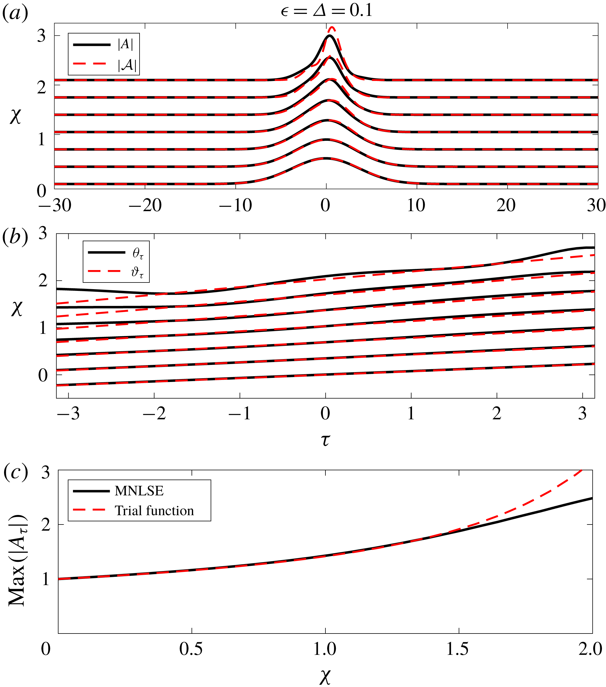
A comparison between numerical simulations of the MNLSE and the predictions of the trial function given by (3.3). Here,
 $\unicode[STIX]{x1D716}=\unicode[STIX]{x1D6E5}=0.1$
. The envelope amplitude is shown in (a), where we see agreement between the trial function and the full solutions during focusing, with the agreement breaking down as the packet slope becomes large. The frequencies are shown in (b), and again the trial functions describe the bulk scale evolution of the phase but do not capture the higher
 $\unicode[STIX]{x1D70F}$
-dependent behaviour. (c) Compares the predictions of the slope of the trial function and the MNLSE, with good agreement found for small values of
 $\unicode[STIX]{x1D712}$
, before the approximation breaks down.

3.3 Numerical simulations of the MNLSE
To better understand these predictions, we now look at several numerical examples. The numerical scheme is a split-step pseudo-spectral method, where the step size is chosen so that the energy is conserved to at least 1 part in
 $10^{6}$
and the mean frequency to 1 part in
 $10^{4}$
. The number of modes was increased until convergence was found. In particular, we use
 $2^{12}$
modes and step sizes of the order of
 $10^{-5}$
.
Note, one of the difficulties in applying ideas from weakly nonlinear narrow banded theory to areas outside of their strict asymptotic region of validity is the choice in defining the (small) parameters
 $\unicode[STIX]{x1D716}$
and
 $\unicode[STIX]{x1D6E5}$
(see the discussion in § 2 of Perlin et al. (Reference Perlin, Choi and Tian2013)). For example, does one define the parameter
 $\unicode[STIX]{x1D716}$
as the initial slope, or the largest slope, as predicted by some theory? A technique used in laboratory experiments is to characterize the packet slope
 $S$
based on the linear prediction of the maximum slope at focusing. This has been shown to be effective in describing the strength of breaking waves for laboratory wave packets (Drazen et al.
Reference Drazen, Melville and Lenain2008), which, due to wave channel length limitations, must be broadband in order to start as linear waves and progress to breaking over a reasonable fetch (usually on the order of
 $10$
m). Based on this, we connect the parameters
 $(\unicode[STIX]{x1D716},\unicode[STIX]{x1D6E5})$
with the predictions of the maximum modulations to amplitude and spatial/temporal scales according to linear theory.
Figure 3 shows a comparison of the predictions of the trial functions with the MNLSE. Here,
 $\unicode[STIX]{x1D716}=\unicode[STIX]{x1D6E5}=0.1$
. We can see good agreement between the predictions of the amplitude
 $|A|$
and the trial function amplitude
 ${\mathcal{A}}=|{\mathcal{A}}|\text{e}^{\text{i}\unicode[STIX]{x1D717}}$
, while the frequency evolution
 $\unicode[STIX]{x1D703}_{\unicode[STIX]{x1D70F}}$
(where we recall
 $A=|A|\text{e}^{\text{i}\unicode[STIX]{x1D703}}$
) agrees with trial function predictions until focusing, when the
 $\unicode[STIX]{x1D70F}$
structure is more complicated than the low-order polynomials we assumed for
 $\unicode[STIX]{x1D717}$
. The lowest row shows the predictions of the magnitude of the envelope slope
 $|A_{\unicode[STIX]{x1D70F}}|$
of the envelope during focusing, and there is relatively good agreement for small values of
 $\unicode[STIX]{x1D712}$
. However, this simple model is unable to predict the slope at focusing, as the asymmetric term is not part of the energy balance to this order and grows secularly.
3.4 Maximum slope at focusing
In this section we seek to model the maximum slope at focusing, based on the initial packet parameters
 $(\unicode[STIX]{x1D716},\unicode[STIX]{x1D6E5})$
. The variational method hinted at the importance of
 $\unicode[STIX]{x1D6FE}_{0},\unicode[STIX]{x1D6FC}_{0},\unicode[STIX]{x1D6FD}_{0}$
in describing the focusing event. In particular, the values of
 $w_{\ast }$
, which we recall is the minimum packet width predicted by the variational method, sets the scale of the envelope at focusing. These values are not uniquely defined as a function of
 $\unicode[STIX]{x1D716},\unicode[STIX]{x1D6E5}$
, and to first order in
 $\unicode[STIX]{x1D716}^{2}/\unicode[STIX]{x1D6E5}$
, it may be seen that when
 $\unicode[STIX]{x1D6E5}=d_{0}\unicode[STIX]{x1D716}+d_{1}\unicode[STIX]{x1D716}^{2}$
, then lines of constant
 $w_{\ast }$
may be found for
 $d_{0}^{2}/2=w_{\ast }(1-w_{\ast })/(4w_{\ast }^{2}-2)$
and
 $d_{1}$
a more complicated function of
 $w_{\ast }$
which is not presented here as it is not relevant for the ensuing discussion. This hints at a quasi self-similarity in the focusing event.
Next, the free surface
 $\unicode[STIX]{x1D702}$
is given by (2.7). To better understand the dependence of max
 $(|\unicode[STIX]{x1D702}_{x}|)$
on
 $(\unicode[STIX]{x1D716},\unicode[STIX]{x1D6E5})$
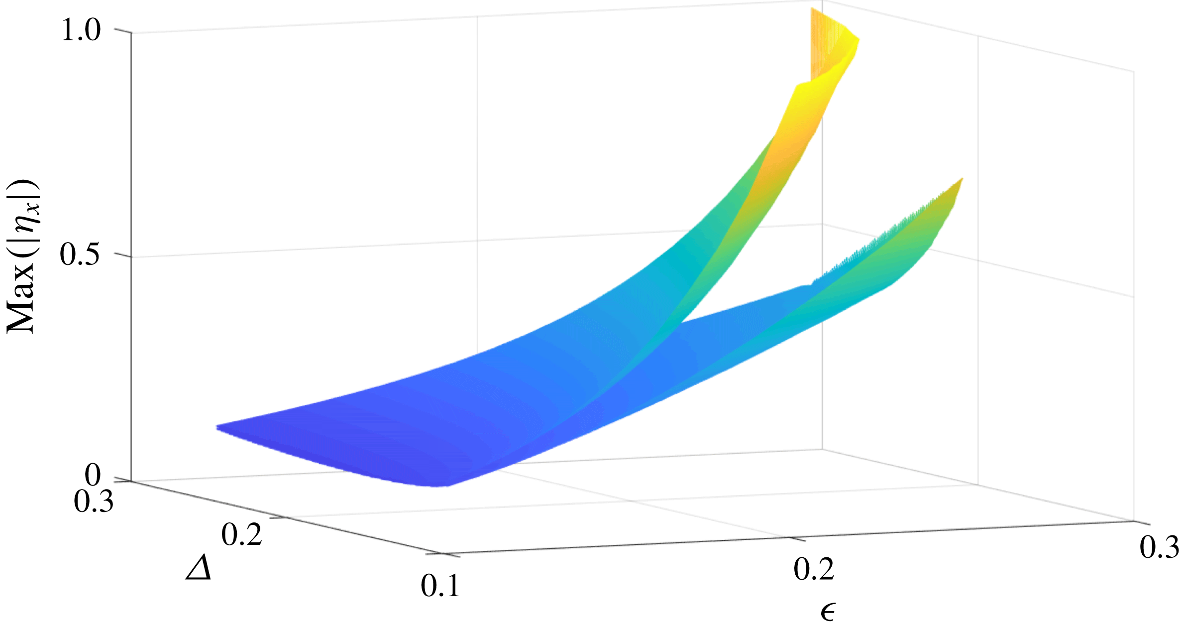
, the MNLSE was numerically integrated with the initial conditions given by (3.1) for 400 values of
 $\unicode[STIX]{x1D716}$
and
 $\unicode[STIX]{x1D6E5}$
, and the maximum of the modulus of the slope is shown in figure 4. Note, the three decibel width of the initial spectrum is chosen as a measure of the packet bandwidth,
 $\unicode[STIX]{x1D6E5}$
. For comparison, the same simulations are conducted for the NLSE and are shown. The slope predictions are larger for the MNLSE, and this becomes more pronounced with increasing
 $\unicode[STIX]{x1D716}$
and decreasing
 $\unicode[STIX]{x1D6E5}$
(which corresponds to increasing
 $\unicode[STIX]{x1D6FE}_{0},\unicode[STIX]{x1D6FC}_{0},\unicode[STIX]{x1D6FD}_{0}$
).
The maximum of the modulus of the slope, max
 $(|\unicode[STIX]{x1D702}_{x}|)$
, according to the modified nonlinear Schrodinger equation (upper surface) and nonlinear Schrodinger equation (lower surface) as a function of
 $\unicode[STIX]{x1D716}$
and
 $\unicode[STIX]{x1D6E5}$
. Here, 400 runs were conducted, and the displayed surfaces are interpolated based on these data points. Note, the MNLSE predicts noticeably larger slopes than its lower-order counterpart, in accordance with the theoretical considerations of § 3. Slopes are largest for large
 $\unicode[STIX]{x1D716}$
and small
 $\unicode[STIX]{x1D6E5}$
, corresponding to larger values of
 $\unicode[STIX]{x1D6FE}_{0},\unicode[STIX]{x1D6FC}_{0},\unicode[STIX]{x1D6FD}_{0}$
.

We define the maximum of the modulus of the free surface slope as
 ${\mathcal{T}}$
, that is
 $$\begin{eqnarray}{\mathcal{T}}\equiv \text{max}(|\unicode[STIX]{x1D702}_{x}|).\end{eqnarray}$$
For linear waves, we have
 ${\mathcal{T}}=\unicode[STIX]{x1D716}$
, by definition. From (3.26), the definition of
 $\unicode[STIX]{x1D702}$
(i.e. (2.7)), and the asymptotic self-similarity of
 $w_{\ast }$
described above, we propose that for the MNLSE
 $$\begin{eqnarray}{\mathcal{T}}=\unicode[STIX]{x1D716}(1+f(\unicode[STIX]{x1D705})),\end{eqnarray}$$
with
 $\unicode[STIX]{x1D705}$
as defined in (3.25) and
 $f$
a function, to be constrained by the numerical simulations.
Next, by inspection of figure 4 we expect the growth of the slope to be sensitive to values of
 $\unicode[STIX]{x1D6FE}_{0}$
and
 $\unicode[STIX]{x1D6FC}_{0}$
. To this end, we assume that the function
 $f$
is exponential, and find the following fit
 $$\begin{eqnarray}{\mathcal{T}}=\unicode[STIX]{x1D716}\left(h_{0}+h_{1}\text{e}^{h_{2}\unicode[STIX]{x1D716}^{2}/\unicode[STIX]{x1D6E5}^{2}(1+h_{3}\unicode[STIX]{x1D6E5})}\right),\end{eqnarray}$$
with
 $(h_{0},h_{1},h_{2},h_{3})=(-0.37,1.18,0.20,10.05)$
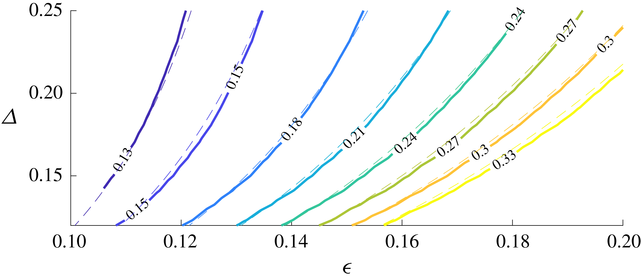
given by a least squares fit with the data. A comparison of this model with the data is shown in figure 5 in the form of a contour plot. There, bulk scale agreement between this simple model and the data is shown. Note, these coefficients also have a dependence on the chirp of the packet
 $C$
.
Finally, note that (3.29) implies
 $$\begin{eqnarray}\unicode[STIX]{x1D6E5}=\frac{h_{2}h_{3}\unicode[STIX]{x1D716}^{2}+\sqrt{h_{2}}\unicode[STIX]{x1D716}\sqrt{4\ln ({\mathcal{T}}/\unicode[STIX]{x1D716}-h_{0})+h_{2}h_{3}^{2}\unicode[STIX]{x1D716}^{2}-4\ln (h_{1})}}{2\ln ({\mathcal{T}}/\unicode[STIX]{x1D716}-h_{0})-2\ln (h_{1})}.\end{eqnarray}$$
A comparison of the contours of max
 $(|\unicode[STIX]{x1D702}_{x}|)$
as a function of
 $(\unicode[STIX]{x1D716},\unicode[STIX]{x1D6E5})$
, with the model
 ${\mathcal{T}}$
(dashed lines) given by (3.29). There is a bulk scale agreement between this relatively simple model and the numerical simulations.

4 Numerical simulations of the fully nonlinear potential flow equations
Motivated by the quasi-self-similarity of focusing in the MNLSE, as well as the success of a simple model in predicting the maximum slope, we now investigate whether or not this may form a breaking criterion. That is, we assume all waves with a local slope that exceed some threshold
 ${\mathcal{T}}_{0}$
break. Specifically, we investigate how well a model of the form given by (3.30) partitions phase space between breaking and non-breaking waves.
To this end, we numerically integrate the equations of motion for fully nonlinear irrotational inviscid deep-water surface gravity waves. The numerical scheme of Dold & Peregrine (Reference Dold and Peregrine1986) is used (see also Dold Reference Dold1992) to study focusing wave packets. This scheme iteratively solves Laplace’s equation by using Cauchy’s integral theorem. Initially,
 $2^{11}$
Lagrangian surface points are distributed along the free surface. Near the focusing point the system is remapped using a conformal mapping technique to increase resolution in this region (Boyd Reference Boyd2001), following similar techniques used in theoretical and numerical studies of Stokes waves (Yamada Reference Yamada1957; Tanaka Reference Tanaka1983; Lushnikov, Dyachenko & Silantyev Reference Lushnikov, Dyachenko and Silantyev2017). In particular, we map our horizontal domain to a unit circle. Then, if the original unit circle was described by
 $z=\text{e}^{\text{i}\unicode[STIX]{x1D701}}$
, the mapped points are given by
 $Z=\text{e}^{\text{i}\unicode[STIX]{x1D6E9}}$
, where
 $$\begin{eqnarray}\unicode[STIX]{x1D6E9}=\frac{\unicode[STIX]{x1D701}+\unicode[STIX]{x1D708}_{0}}{1+\unicode[STIX]{x1D708}_{0}\unicode[STIX]{x1D701}};\quad -1<\unicode[STIX]{x1D708}_{0}\leqslant 0,\end{eqnarray}$$
where
 $\unicode[STIX]{x1D708}_{0}$
is a parameter prescribing how much to contract the region near
 $\unicode[STIX]{x1D701}=\unicode[STIX]{x03C0}$
and stretch near
 $\unicode[STIX]{x1D701}=0$
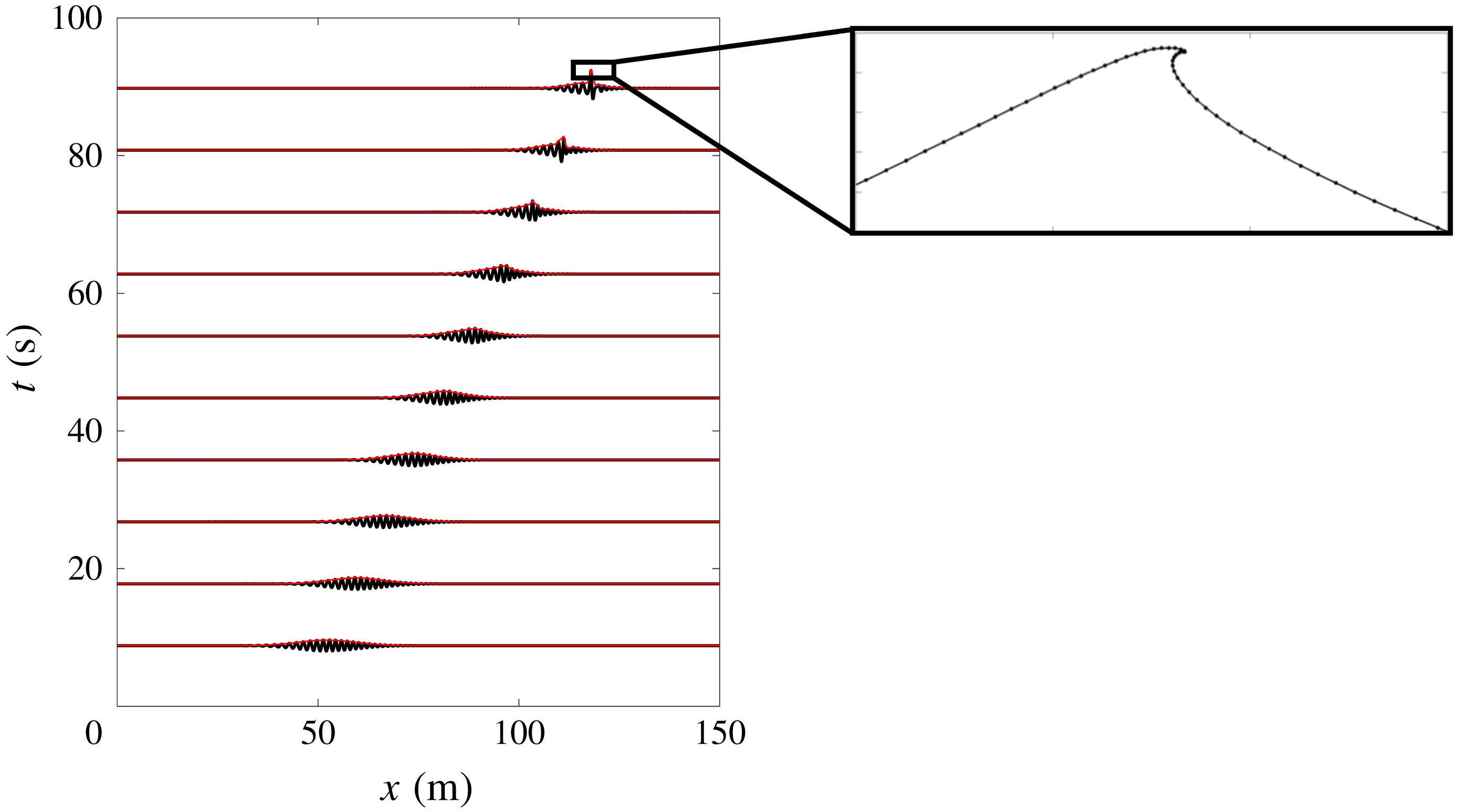
. We may shift this region to coincide with areas of maximum steepness, hence increasing the resolution in this region. We may also apply this mapping iteratively, to capture the fine scale structure of the free surface geometry near breaking. An example of this is shown in the inset of figure 6.
The packet evolution in the numerical simulations of the fully nonlinear potential flow equations, for
 $\unicode[STIX]{x1D716}=0.18$
and
 $\unicode[STIX]{x1D6E5}=0.24$
. A chirped packet uses dispersive focusing, so that longer faster waves catch up to shorter slower waves, leading to energy localization and in this case wave breaking. The free surface displacement
 $\unicode[STIX]{x1D702}$
is shown black, while the packet envelope is shown in red. Note the asymmetric self-steepening on the forward face of the envelope and the amplitude amplification. The inset shows the breaking event after the particle locations have been remapped, with the particle locations shown by the black dots.

Our general numerical program is to run each simulation until the free surface curvature exceeds a threshold value, which is an indication that breaking might be occurring. Each simulation, regardless of whether or not breaking was suspected, is then rerun, starting one wave period before the largest magnitude of the observed slope. The mapping, i.e. equation (4.1), is then applied. We subsequently examined whether or not a wave in the packet has broken, where we say a wave has broken if the free surface becomes multivalued. Furthermore, we ensure that the total energy is conserved in this mapping to at least one part in
 $10^{6}$
.
This technique allows us to create a numerical wave tank that resolves the jet of the breaking wave, and gives us the ability to accurately compute the geometry and kinematics of these waves at breaking. This offers significant advantages over large eddy simulations (Derakhti & Kirby Reference Derakhti and Kirby2016; Derakhti, Banner & Kirby Reference Derakhti, Banner and Kirby2018) which accurately capture post breaking bulk scale quantities and offer an insightful tool to study these integral properties, but suffer from poor resolution of the geometry of the free surface near breaking and hence also the free surface kinematics (Pizzo Reference Pizzo2017).
As our initial conditions, following laboratory studies (Longuet-Higgins Reference Longuet-Higgins1974; Rapp & Melville Reference Rapp and Melville1990), we use a dispersive focusing technique to localize energy density in space and time, possibly leading to wave breaking. These packets allow for future comparison with laboratory data, and enables us to test how well the predictions made in § 3 work for wave packets that are not explicitly chirped Gaussian packets.
The wave packets are of the form
 $$\begin{eqnarray}\unicode[STIX]{x1D702}=\mathop{\sum }_{n=1}^{N}a_{n}\cos (k_{n}(x-x_{b})-\unicode[STIX]{x1D714}_{n}(t-t_{b})),\end{eqnarray}$$
where
 $N$
is the number of waves, taken to be
 $32$
here (Drazen et al.
Reference Drazen, Melville and Lenain2008),
 $x_{b}$
and
 $t_{b}$
are the distance and time to focusing, with
 $t_{b}=c_{g}^{-1}x_{b}$
, while
 $\unicode[STIX]{x1D714}_{n}$
and
 $k_{n}$
are the frequency and wavenumber for each component, connected via the linear dispersion relationship
 $\unicode[STIX]{x1D714}_{n}^{2}=gk_{n}$
. The wavenumbers are chosen so that
 $k_{n}=k_{0}(1+\unicode[STIX]{x1D6FF}(n-1)/N)$
for
 $\unicode[STIX]{x1D6FF}$
a constant related to the packet bandwidth.
Two parameters describe these wave packets. First, the linear prediction of the maximum slope at breaking is given by
 $$\begin{eqnarray}S=\mathop{\sum }_{n=1}^{N}a_{n}k_{n}.\end{eqnarray}$$
Next, the packet bandwidth is set by the parameter
 $\unicode[STIX]{x1D6FF}$
, as well as a windowing function that ensures that just one (initially compact) wave packet is generated (Rapp & Melville Reference Rapp and Melville1990). The three decibel width of the initial spectrum is chosen as a measure of the packet bandwidth,
 $\unicode[STIX]{x1D6E5}$
. The distance to breaking,
 $x_{b}$
is chosen so that
 $x_{b}=5(\unicode[STIX]{x1D6FF}k_{0})^{-1}$
which ensures that the original packet is linear (and the bound component contributions are initially negligible) and we take
 $f_{0}=1$
Hz.
An example of packet evolution in these numerical integrations is shown in figure 6. The black lines show the free surface elevation, while the red lines show the wave envelope evolution, found via the Hilbert transform (Melville Reference Melville1983). The focusing process is marked by a strong asymmetric self-steepening on the forward face of the packet, eventually leading to wave breaking, which is shown in the figure inset.
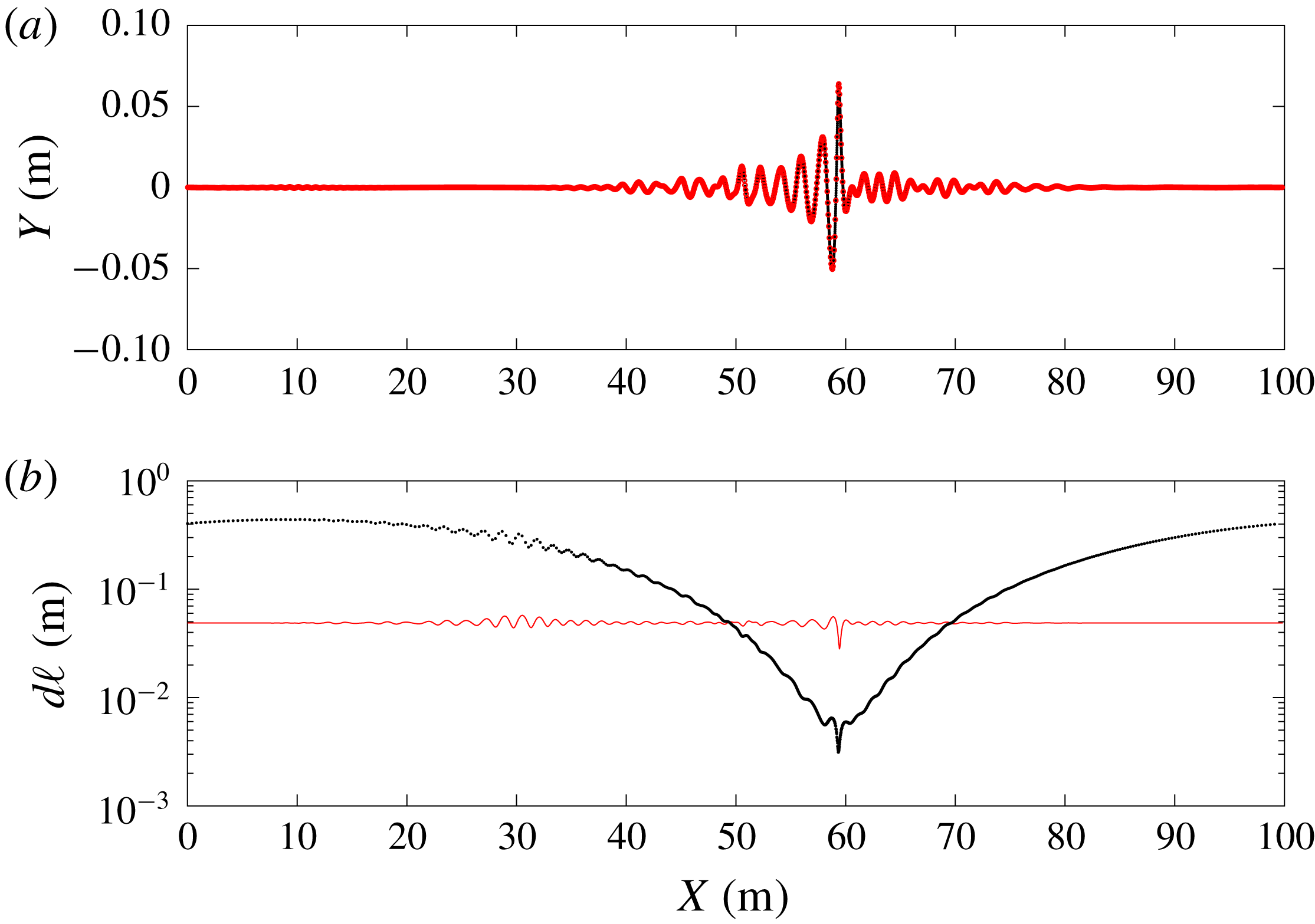
Near focusing, the particle locations are remapped using (4.1), so that they become more dense in the region of largest slope magnitude. This is shown in figure 7. In figure 7(a), the original mapping is shown in red, while the re-mapped particles are shown in black, where
 $\unicode[STIX]{x1D708}_{0}$
was taken to be
 $-0.5$
. The distance between adjacent particles,
 $d\ell$
, is then shown in figure 7(b) where it is seen that the resolution is enhanced by nearly an order of magnitude in this focusing region. This allows us to accurately capture the free surface geometry, which is crucial for detecting wave breaking.
(a) The particle locations in the original integration are shown in red, while the mapped particle locations are shown in black. Here,
 $\unicode[STIX]{x1D708}_{0}=-0.5$
in the conformal mapping given by (4.1)). The distance between adjacent particles in the original scheme (red) and the mapped coordinates (black). The resolution has been increased by nearly an order of magnitude near the steepest part of the wave using this technique.

We now perform 80 integrations of different initial conditions exploring the
 $(\unicode[STIX]{x1D716},\unicode[STIX]{x1D6E5})$
phase space, where following the above discussion we take
 $\unicode[STIX]{x1D716}$
to be
 $S$
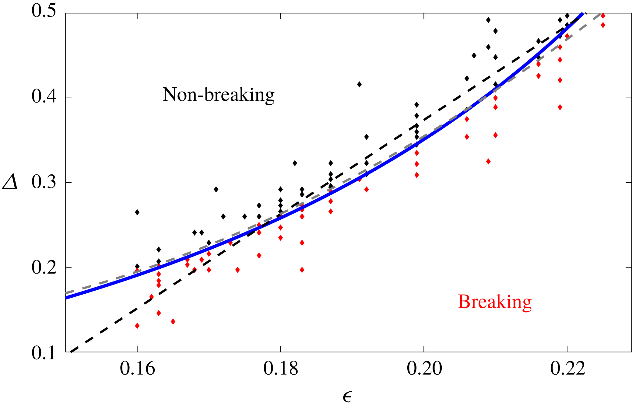
, the linear prediction of the maximum slope at focusing. The phase space is partitioned between breaking and non-breaking waves, as is shown in figure 8. We plot
 $$\begin{eqnarray}\unicode[STIX]{x1D6E5}=\unicode[STIX]{x1D709}_{0}\frac{h_{3}h_{4}\unicode[STIX]{x1D716}^{2}+\sqrt{h_{3}}\unicode[STIX]{x1D716}\sqrt{4\ln ({\mathcal{T}}/\unicode[STIX]{x1D716}-h_{0})+h_{3}h_{4}^{2}\unicode[STIX]{x1D716}^{2}-4\ln (h_{1})}}{2\ln ({\mathcal{T}}/\unicode[STIX]{x1D716}-h_{0})-2\ln (h_{1})},\end{eqnarray}$$
where
 $\unicode[STIX]{x1D709}_{0}$
is best fit to the data with value
 $1.28$
. The blue line shows the prediction of our model with
 ${\mathcal{T}}=0.28$
, while the black dashed line shows a linear best fit to the data and the grey line shows the best fit of the data to a quadratic function.
Top: numerical simulations of various initial bandwidths,
 $\unicode[STIX]{x1D6E5}$
, and linear predictions of the maximum slope at focusing,
 $\unicode[STIX]{x1D716}$
. Red circles are wave packets with breaking, while those in black are wave packets where no breaking was observed. There is a distinct partitioning of this phase space between these two types of evolution. The model given by (4.4) is shown by the blue line, and describes the bulk scale partitioning of phase space between breaking and non-breaking waves, while the black line is a linear best to the data and the grey line shows the best fit to a quadratic polynomial in
 $\unicode[STIX]{x1D716}$
.

We notice bulk scale agreement between the model and the numerical simulations. For larger values of
 $\unicode[STIX]{x1D716}$
and
 $\unicode[STIX]{x1D6E5}$
the fit breaks down, as higher-order descriptions are needed to accurately predict the local slope (cf. (2.7)). Furthermore, the fine scale partitioning is not captured. Nevertheless, the bulk scale behaviour appears to be quasi-self-similar, and the models serves as a simple coarse description of the partitioning in phase space of breaking and non-breaking focusing chirped wave packets.
5 Conclusion
Near the peak of the spectrum, it is believed that wave–wave interactions are an important cause of wave breaking (Rapp & Melville Reference Rapp and Melville1990). Therefore, the chirped packets considered here serve as a model of these types of breaking events, highlighting the importance of the entire group structure in determining whether or not a wave breaks. This simple description of breaking may be used in more sophisticated statistical models of wave field evolution, where a local estimate of wave slope and bandwidth may be used together with the criterion given by (4.4) to quantify the breaking statistics. Coupled with recent field measurements of these breaking statistics (Sutherland & Melville Reference Sutherland and Melville2013, Reference Sutherland and Melville2015), this may serve as an important constraint on models of the statistics of the surface wave field. Furthermore, this result may then be included in scaling arguments describing the breaking induced flow (e.g. the energy dissipation (Drazen et al. Reference Drazen, Melville and Lenain2008), the circulation induced by breaking (Pizzo & Melville Reference Pizzo and Melville2013) and the mass transport induced by breaking (Deike, Pizzo & Melville Reference Deike, Pizzo and Melville2017; Pizzo, Melville & Deike Reference Pizzo, Melville and Deike2019) to better describe the observations.
Despite the limitations of using a weakly nonlinear narrow-banded waves to examine wave breaking in deep-water surface gravity waves, the way to interpret the model presented in this paper is that it provides a simple qualitative description of the physics that can lead an initially symmetric wave packet up to the point where large gradients are expected in the free surface displacement, and breaking is likely. The results are studied numerically, and there is a bulk scale partitioning of phase space between non-breaking and breaking waves, which may be described by a model motivated by analysis of the quasi self-similarity found in focusing wave packets governed by the MNLSE.
Acknowledgement
This research was supported by grants to W.K.M. from the National Science Foundation (Physical Oceanography) and the Office of Naval Research. N.P. thanks the Kavli Institute for Theoretical Physics (supported by the National Science Foundation under grant no. NSF PHY17-48958), where part of this research was conducted. We also thank four anonymous referees, whose comments have led to significant improvements to the manuscript.