




1. Introduction
Reliable estimation of galaxy redshift is critical for mapping the large-scale structure of the Universe, constraining cosmological parameters, and understanding galaxy formation and evolution. To infer redshift, two primary sources of data have been used: photometric observations and spectroscopic observations. Obtaining and analyzing spectroscopic measurements provides reliable estimates; however, this reliability comes at the price of increased instrument complexity, telescope time, and complex data reduction pipelines (Abolfathi et al. Reference Abolfathi2018; Laureijs et al. Reference Laureijs2011). Photometric redshift estimation (photo-z) offers an attractive alternative by inferring redshift from fluxes measured in a small number of broadband filters (Bolzonella et al. Reference Bolzonella, Miralles and Pelló2000), enabling the fast and cost-efficient acquisition of relevant observations. However, the increased efficiency comes at the expense of reduced accuracy and the presence of systematic biases.
Over the past two decades, a wide range of methods for photometric and spectroscopic redshift estimation have been proposed, ranging from template-fitting approaches (Bolzonella et al. Reference Bolzonella, Miralles and Pelló2000) to machine learning–based methods (Collister and Lahav Reference Collister and Lahav2004; Carliles et al. Reference Carliles, Budavári, Heinis, Priebe and Szalay2010; Beck et al. Reference Beck, Lin and Ishida2017; Stivaktakis et al. Reference Stivaktakis, Tsagkatakis and Tsakalides2020). While these techniques have greatly improved the performance of photometric redshifts, major challenges remain. One such challenge is the reliable characterization of prediction uncertainty. Uncertainty quantification (UQ) is critical for cosmological applications of photometric redshifts. In weak gravitational lensing and large-scale structure studies, for instance, even small mischaracterizations of redshift distributions can lead to biased cosmological parameter estimates (Mandelbaum et al. Reference Mandelbaum, Seljak and Hirata2008; Sánchez et al. Reference Sánchez, Carrasco Kind and Lin2014). UQ can be broadly classified into two classes. Epistemic or model uncertainty stems from limited knowledge or data and, in principle, can be reduced with more or better data/modeling. Aleatoric or data uncertainty arises from inherent variability of the signals, e.g., noise, and is irreducible even with unlimited data. While recent works have explored probabilistic methods for photo-z estimation (Malz and Hogg Reference Malz and Hogg2022; Dalmasso et al. Reference Dalmasso, Pospisil, Lee, Izbicki, Freeman and Malz2020), there remains no consensus on the most effective strategy for delivering reliable and interpretable redshift probability distributions.
In this work, we systematically evaluate a suite of uncertainty-aware machine learning approaches for photometric redshift estimation using Sloan Digital Sky Survey (SDSS) data. We focus on aleatoric uncertainty, evaluating techniques including Gaussian regression, quantile regression, conformalized regression prediction. Our results highlight the benefits of these approaches and demonstrate how incorporating uncertainty estimates improves the robustness of photometric redshift predictions.
2. Methods
2.1. Baseline point-like estimation
We formulate photometric redshift estimation as a supervised regression problem, where the goal is to predict the redshift
 $y_i$
of a galaxy from its photometric features
 $x_i$
. As a baseline, we consider a feed-forward multi-layer perceptron (MLP) network that outputs a single-point estimate of the redshift. The baseline model is defined as
 $\hat{y}_i = f(x_i; \mathbf{w})$
where
 $f(\cdot;\mathbf{w})$
is the neural network parameterized by weights
 $\mathbf{w}$
,
 $\hat{y}_i$
is the prediction for the i-th galaxy, and
 $y_i$
is the corresponding ground-truth spectroscopic redshift. In this work, we consider a compact two-hidden-layer network following the MLP architecture with 128 units per layer, and a ReLU activation function. The network is trained by minimizing the mean squared error (MSE)
 \begin{equation*} \text{MSE} = \frac{1}{n} \sum_{i=1}^n (f(x_i; \mathbf{w}) - y_i)^2\end{equation*}
The model is optimized with Adam (learning rate
 $10^{-4}$
) using mini-batches of size 1024.
2.2. Gaussian regression via ANN
In Gaussian regression, the ANN outputs a mean
 $\mu_i$
and a variance
 $\sigma_i^2$
for each input
 $x_i$
, modeling heteroscedastic (input-dependent) aleatoric uncertainty. Formally, for each i we assume
 $y_i \mid x_i \sim \mathscr{N}(\mu_i,\sigma_i^2)$
, so the likelihood for each observation is given by
 \begin{equation*}p(y_i \mid x_i,\mathbf{w})=\frac{1}{\sqrt{2\pi\,\sigma_i^2}} \exp\!\left(-\frac{(y_i-\mu_i)^2}{2\,\sigma_i^2}\right).\end{equation*}
Training is performed by minimizing the mean negative log-likelihood (NLL) over N observations:
 \begin{equation*}\mathscr{L}(\mathbf{w})= \frac{1}{N}\sum_{i=1}^{N}\left[\frac{1}{2}\log\!\big(2\pi\,\sigma_i^2\big)+ \frac{(y_i-\mu_i)^2}{2\,\sigma_i^2}\right].\end{equation*}
To improve numerical stability we bound the predicted standard deviations via clipping to prevent degenerate solutions.
2.3. Quantile regression
Instead of a parametric distribution, in the case of quantile regression, the network predicts conditional quantiles (e.g., 5th and 95th percentiles). Formally, we assume a set of target quantiles
 $\{\alpha_k\}_{k=1}^{K}$
where
 $ \hat{\mathbf{y}}_i = f(x_i;\mathbf{w}) = \bigl(\hat{y}_{i,\alpha_1},\,\hat{y}_{i,\alpha_2},\,\dots,\,\hat{y}_{i,\alpha_K}\bigr)$
Training minimizes the pinball loss:
 \begin{equation*}L_{\alpha}\bigl(y,f(x)\bigr)\;=\;\begin{cases} \alpha\,\lvert y - f(x) \rvert, & y \ge f(x),\\[4pt] (1-\alpha)\,\lvert y - f(x) \rvert, & y < f(x).\end{cases}\end{equation*}
This enables the network to approximate arbitrary predictive distributions and provides asymmetric uncertainty estimates.
2.4. Conformal Prediction
Conformal methods wrap around point or quantile predictors to deliver finite-sample, distribution-free coverage guarantees under exchangeability. We adopt conformalized quantile regression (CQR), which calibrates quantile regression intervals using a held-out calibration set (Romano et al. Reference Romano, Patterson and Candès2019). The procedure is as follows:
-
(1) Split the training data into a proper training set and a calibration set.
-
(2) Train lower- and upper-quantile regressors
 $\widehat{Q}^{\alpha/2}$
and
$\widehat{Q}^{\,1-\alpha/2}$
on the proper training set.
-
(3) On the calibration set, compute conformity scores
\begin{equation*} s_i^{\text{CQR}} = \max\!\Bigl\{ \widehat{Q}^{\alpha/2}(x_i^{c}) - y_i^{c}, \; y_i^{c} - \widehat{Q}^{\,1-\alpha/2}(x_i^{c}), \; 0 \Bigr\}. \end{equation*}
-
(4) Let
$s^{\text{CQR}}_{(1)} \le \cdots \le s^{\text{CQR}}_{(n^{c})}$
denote the sorted calibration scores. Compute the
$(1-\alpha) (1+1/n^{c})$
-quantile:
\begin{equation*} k = \Bigl\lceil (1-\alpha)(n^{c}+1)\Bigr\rceil, \qquad \widehat{q}^{\text{CQR}} = s^{\text{CQR}}_{(k)}. \end{equation*}
-
(5) Output the prediction interval for a new input x:
\[ \mathscr{C}^{\text{CQR}}(x) = \Bigl[ \widehat{Q}^{\alpha/2}(x)-\widehat{q}^{\text{CQR}},\; \widehat{Q}^{\,1-\alpha/2}(x)+\widehat{q}^{\text{CQR}} \Bigr]. \]


This procedure guarantees marginal coverage at the desired level
 $1-\alpha$
under the assumption of exchangeability, independent of the underlying data distribution.
3. Experimental Analysis
3.1. Dataset
We consider photometric observations and spectroscopically estimated redshifts from the Sloan Digital Sky Survey (SDSS) Data Release 16 (DR16) (Ahumada et al. Reference Ahumada, Prieto, Almeida, Anders, Anderson, Andrews, Anguiano, Arcodia, Armengaud and Aubert2020). We restrict the sample to sources with spectroscopic redshifts in the range
 $0 \leq z \leq 0.31$
, which represents the bulk of low-redshift SDSS galaxies. The photometric input features consist of broadband magnitudes in the u, g, r, and i bands. After quality filtering, the dataset was randomly split into 800,000 training samples and 200,000 validation samples. All features were standardized to zero mean and unit variance prior to training.
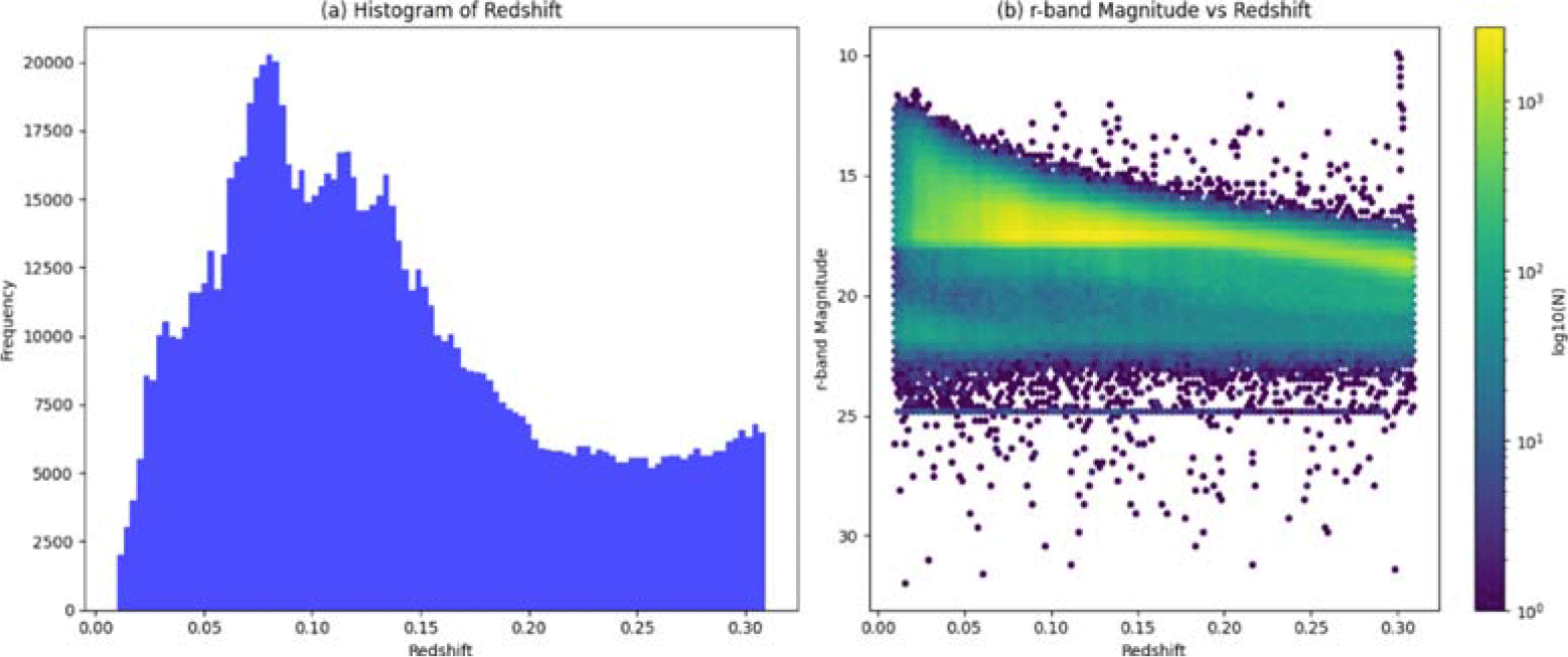
Figure 1 (a) shows the distribution of spectroscopic redshifts in the dataset, with a strong concentration of galaxies at low redshift and a gradual decline towards higher values. Figure 1 (b) complements this view by depicting the relation between r-band magnitude and redshift. The plot highlights the observational selection effects of the survey: brighter galaxies dominate at lower redshifts, while at higher redshifts the sample is restricted to intrinsically brighter objects due to the flux limit of the SDSS.
(a) Distribution of galaxy redshifts in the SDSS dataset. (b) Relation between r-band magnitude and redshift, showing observational selection effects.

3.2. Experimental results
3.2.1. Baseline point estimation
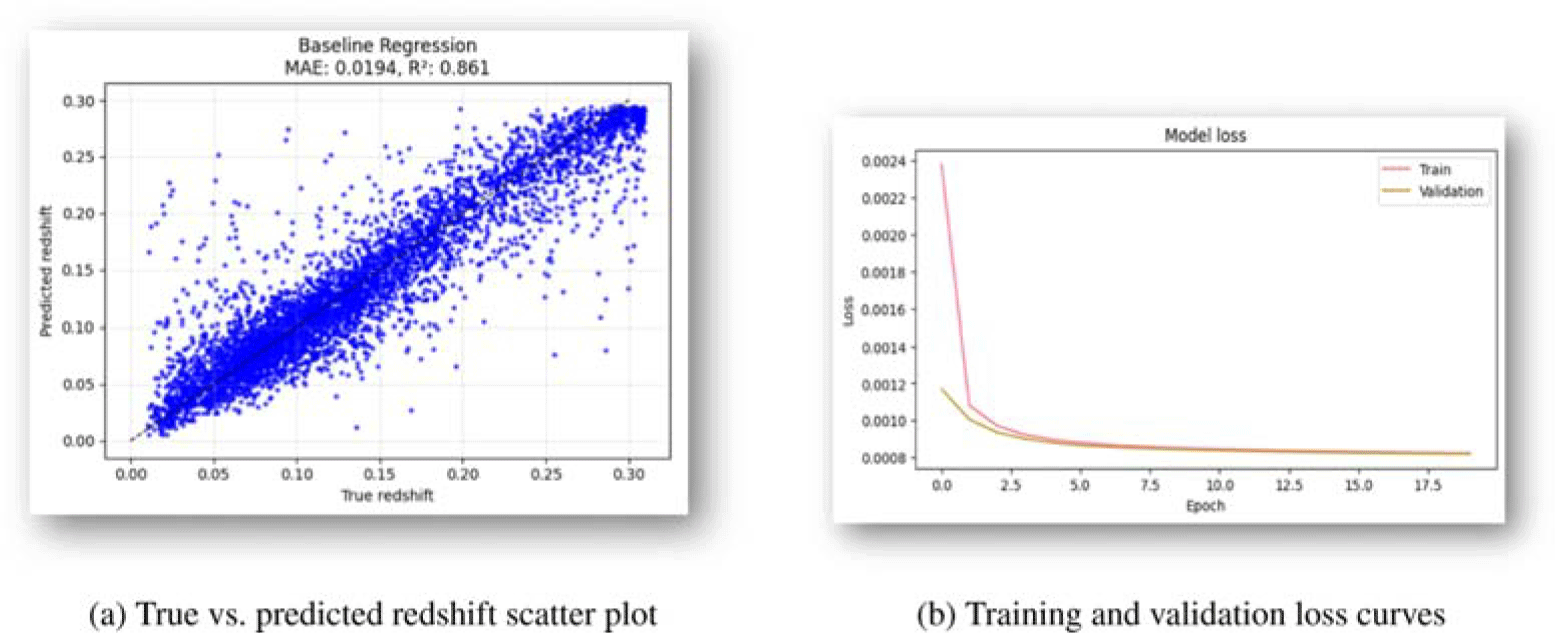
The performance of the baseline point-estimation ANN is illustrated in Figure 2(a), which shows the scatter plot of predicted versus true redshifts. The distribution of points closely follows the diagonal, indicating that the network captures the general mapping between photometric features and redshift effectively. Quantitatively, the model achieves a mean absolute error (MAE) of 0.0194 and a coefficient of determination (
 $R^2$
) of 0.861, confirming that the baseline ANN provides accurate photometric redshift predictions. Furthermore, the evolution of the training and validation loss does not indicate signs of overfitting as demonstrated in Figure 2(b). Nonetheless, systematic deviations are evident. A noticeable scatter around the diagonal reveals that for a subset of galaxies, redshifts are either under- or over-estimated. These discrepancies are more pronounced at higher redshifts and for objects with noisier photometric measurements, consistent with the distributional biases highlighted in Figure 1.
Performance of the baseline ANN model. (a) Scatter plot of predicted vs. true redshifts. (b) Training and validation loss over epochs.

3.2.2. Gaussian Regression
To obtain both point predictions and per-object uncertainty, we train a network to output a mean
 $\hat{\mu}(x)$
and a standard deviation
 $\hat{\sigma}(x)$
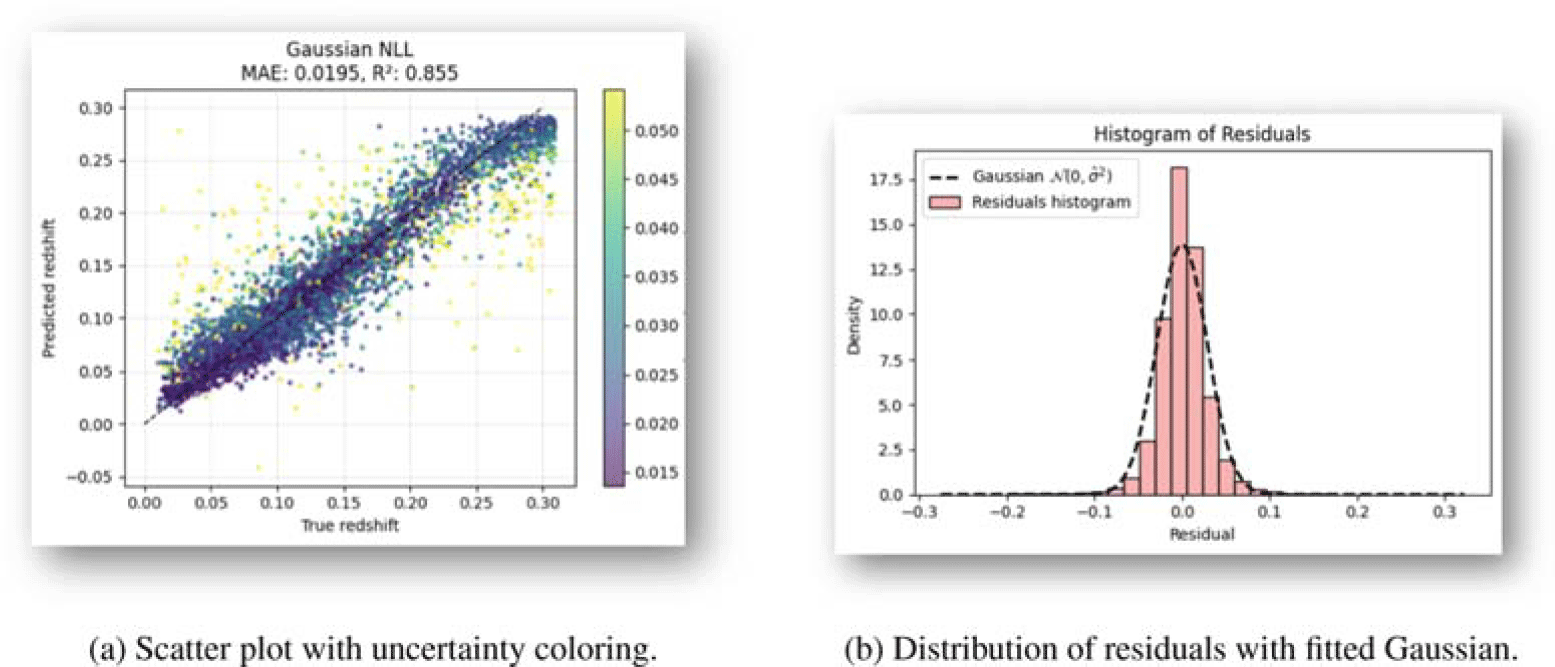
and optimize the Gaussian negative log-likelihood. Figure 3(a) shows the scatter of predicted versus true redshift, with points color-coded by the predicted uncertainty
 ${R^2 = 0.855}$
(lighter colors indicate larger uncertainty). The model achieves MAE = 0.0195 and
 $\hat{\sigma}(x)$
, which is comparable to the baseline point estimator, while additionally providing an uncertainty estimate for each sample. As expected, larger predicted uncertainties tend to occur where the mapping is more challenging (e.g., toward higher redshift and regions with sparser coverage in feature space), and points with higher
 $\hat{\sigma}(x)$
exhibit larger deviations from the diagonal.
Gaussian regression analysis. (a) Scatter plot scale. (b) Histogram of residuals.

Despite the model’s ability to capture some variability, the underlying Gaussianity assumption may not be valid in actual measurements. This observation is manifested in Figure 3(b), where the distribution of residuals exhibits noticeable deviations from a Gaussian shape.
3.2.3. Conformalized Quantile Regression
Figure 4(a) presents the scatter plot for the case of vanilla quantile regression, where the model directly estimates conditional quantiles of the redshift distribution given the photometric inputs. This approach captures the heteroscedastic nature of the prediction problem by providing intervals that vary in size depending on the input. However, the method does not guarantee that the true redshift lies within the predicted interval at the nominal coverage level.
Comparison of (a) Quantile Regression and (b) Conformalized Quantile Regression.

In contrast, Figure 4(b) shows the results obtained using Conformalized Quantile Regression (CQR), where the intervals from quantile regression are calibrated on a held-out calibration set. This conformalization step ensures statistically valid coverage guarantees under minimal assumptions, leading to more reliable uncertainty estimates across the dataset. While the MAE and
 $R^2$
values remain comparable to the vanilla quantile regression case, the conformalized intervals are more robust, particularly in regions of the feature space where the base model tends to under- or over-estimate uncertainty.
4. Conclusions
We presented an investigation of uncertainty-aware machine learning methods for photometric redshift estimation using SDSS data. Starting from a baseline neural network, we explored Gaussian regression, quantile regression, and conformalized quantile regression. Our results indicate that while the baseline model achieves competitive accuracy, uncertainty-aware methods provide more reliable and interpretable predictions. In particular, conformalized quantile regression delivers calibrated intervals with minimal computational cost.
Acknowledgements
This work was supported by the TITAN ERA Chair project (contract no. 101086741) within the Horizon Europe Framework Program of the European Commission. The author acknowledges the use of data from the Sloan Digital Sky Survey (SDSS).
Reproducibility
All code and data used in this work are publicly available at https://github.com/TITAN-Project-EU/PhotoZ_SDSS_ML


 Open access

