1 Introduction
The Julia set of an entire function
 $f: \mathbb {C} \rightarrow \mathbb {C}$
, denoted by
 $\mathcal {J}(f)$
, is the set of points at which the dynamical system
 $(f, \mathbb {C})$
behaves chaotically. The behavior of f near
 $\infty $
plays an important role, and one has the following dichotomy. Either
 $\infty $
is a removable singularity, in which case, f is a polynomial, or
 $\infty $
is an essential singularity, in which case, f is a transcendental entire function.
When f is a polynomial,
 $\mathcal {J}(f)$
is usually small in the sense of Hausdorff dimension. Hausdorff dimension is the most well-studied measure of size for Julia sets, and this is the measure we will study in this manuscript. For instance, one has that the quadratic polynomial
 $p_c(z):=z^2+c$
satisfies
 $\text {dim}(\mathcal {J}(p_c))<2$
for generic
 $c\in \mathbb {C}$
(see for instance [Reference UrbańskiUrb94]), although there exist parameters c satisfying
 $\text {dim}(\mathcal {J}(p_c))=2$
[Reference ShishikuraShi98] and even
 $\text {area}(\mathcal {J}(p_c))>0$
[Reference Avila and LyubichAL22, Reference Buff and ChéritatBC12].
However, when f is a transcendental entire function, the generic situation is that
 $\text {dim}(\mathcal {J}(f))=2$
. For instance, in [Reference MisiurewiczMis81], it was shown that
 $\mathcal {J}(e^z)=\mathbb {C}$
, and in [Reference McMullenMcM87], it was shown that functions in certain standard exponential and sine families have Julia sets of dimension
 $2$
. Thus, in contrast with the polynomial setting, the difficulty in the transcendental setting is to find Julia sets of small dimension, a problem whose history we overview briefly now.
In [Reference BakerBak75], it was proven that the Julia set of any transcendental f must contain a non-trivial continuum and, hence, we always have
 $\text {dim}(\mathcal {J}(f))\geq 1$
. In the class of transcendental f with bounded singular set, denoted
 $\mathcal {B}$
, it was shown in [Reference StallardSta91, Reference StallardSta96, Reference StallardSta00] that
 $$ \begin{align*} \{ \text{dim}(\mathcal{J}(f)) : f \in \mathcal{B} \} = (1,2], \end{align*} $$
(see also [Reference Albrecht and BishopAB20]). Finally, in [Reference BishopBis18], it was proven that outside of the class
 $\mathcal {B}$
, the lower bound of
 $1$
in the inequality
 $\text {dim}(\mathcal {J}(f))\geq 1$
is actually attained (see also [Reference BurkartBur21, Reference ZhangZha24]). Our main result (see Theorem 1.1 below) also achieves this lower bound, but by different methods and with different resulting dynamical properties that we now discuss.
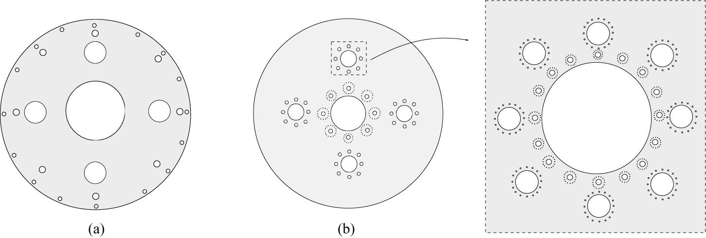
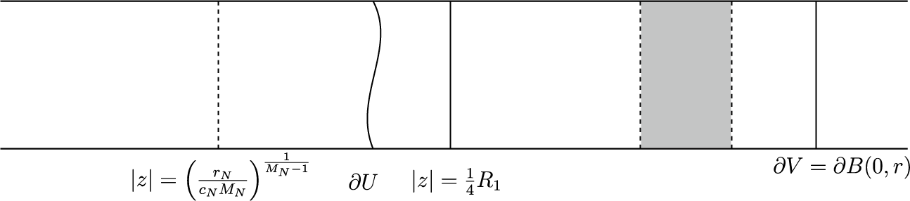
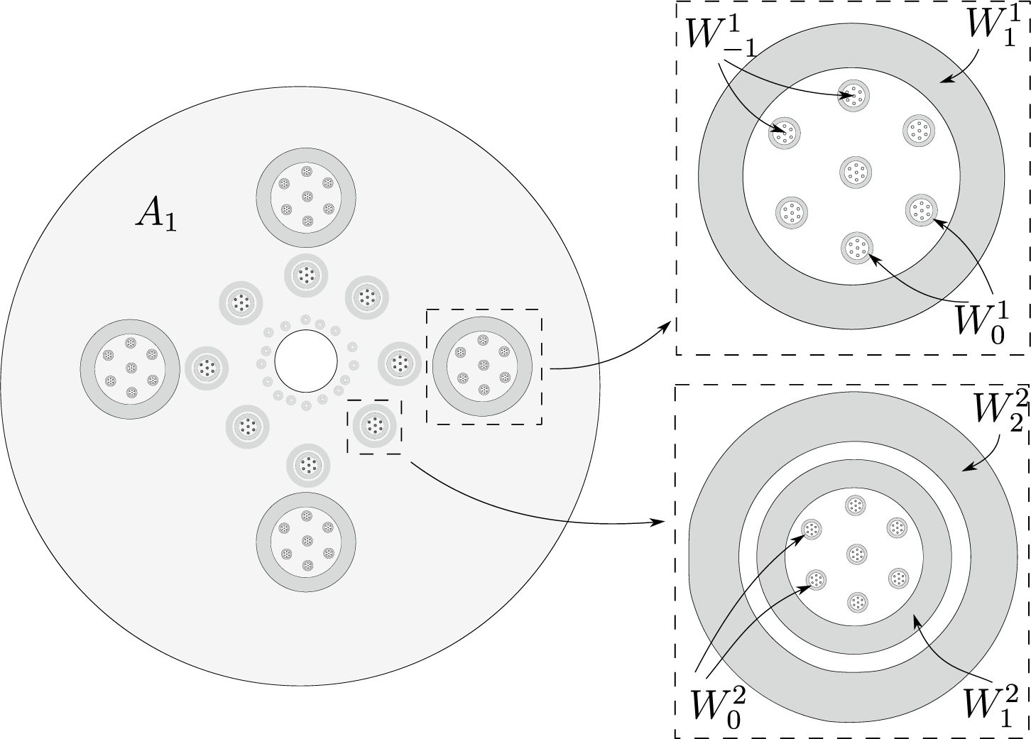
The Fatou set of the function in [Reference BishopBis18] is in fact completely described: it consists of a collection of multiply connected wandering domains, abbreviated m.c.w.d. This class of Fatou components has been well studied [Reference BergweilerBer11, Reference Bergweiler, Rippon and StallardBRS13, Reference Benini, Rippon and StallardBRS16, Reference Bergweiler and ZhengBZ11, Reference FerreiraFer22, Reference Kisaka and ShishikuraKS08, Reference Rippon and StallardRS08, Reference Rippon and StallardRS19] and appears in several different contexts in transcendental dynamics. An m.c.w.d. U of [Reference BishopBis18] consists of a topological annulus minus countably many discs that accumulate only on the outer boundary of U (see Figure 1(a)). This topological structure is aptly termed infinite outer connectivity (defined precisely in [Reference Bergweiler, Rippon and StallardBRS13]). The Fatou components of the function in our Theorem 1.1 are also all m.c.w.d.s; however, they have infinite inner connectivity (see Figure 1(b)), and we prove they have the following more intricate topological structure.
Theorem 1.1. There exists a transcendental entire function
 $f: \mathbb {C} \rightarrow \mathbb {C}$
satisfying:
-
(1)
 $\mathrm {dim}(\mathcal {J}(f))=1$
;
-
(2) each Fatou component of f is a m.c.w.d. of infinite inner-connectivity; and
-
(3) each m.c.w.d. of f has uncountably many singleton complementary components.

Panels (a) and (b) illustrate the concept of infinite outer-connectivity and infinite inner-connectivity, respectively. Panels (a) and (b) also accurately describe the topology of the m.c.w.d.s in [Reference BishopBis18] and Theorem 1.1, respectively. As seen, the structure in panel (b) is more intricate.

Part (3) of Theorem 1.1 answers a question of [Reference Rippon and StallardRS19] (see [Reference Rippon and StallardRS19, Question 9.5]) on the structure of m.c.w.d.s. It is left open whether part (3) in fact must always occur for an m.c.w.d. of infinite inner-connectivity. Another intriguing question suggested by Theorem 1.1 is whether there exist transcendental f with
 $\text {dim}(\mathcal {J}(f))=1$
and doubly connected m.c.w.d.: this is closely related to [Reference BishopBis18, Question 7].
Much of the contribution of the present manuscript is in providing an alternative approach to the breakthrough result of [Reference BishopBis18] (part (1) in Theorem 1.1), an approach that the authors find conceptual and readily adaptable to other settings. The function f of [Reference BishopBis18] is defined by an infinite product that is roughly designed to behave as a monomial on large portions of
 $\mathbb {C}$
. The technical work in describing the dynamics of f relies on formula-heavy estimates of the behavior of f by certain terms in the infinite product.
The approach in the present manuscript is similar in that it constructs f that is designed to behave as a monomial on large portions of
 $\mathbb {C}$
; however, this is done by quasiconformal methods. Namely, a quasiregular
 $h: \mathbb {C} \rightarrow \mathbb {C}$
is constructed, so that by the measurable Riemann mapping theorem, there exists a quasiconformal
 $\phi : \mathbb {C} \rightarrow \mathbb {C}$
such that
 ${f:=h\circ \phi ^{-1}}$
is the entire function of Theorem 1.1. One has freedom in prescribing the dynamics of h, and so the difficulty of describing the dynamics of f becomes a matter of estimating the ‘correction’ map
 $\phi $
, rather than on formula estimates as in [Reference BishopBis18]. The details of this quasiconformal approach were detailed in [Reference Burkart and LazebnikBL23], and has other applications besides that described in the present manuscript.
The advantages of the quasiconformal approach are usually technical in nature. For instance, a key aspect of the proof of Theorem 1.1 is in understanding the location of critical values of f. In [Reference BishopBis18], this requires a delicate estimate involving the infinite product formula. In the quasiconformal approach, this is almost trivial since the critical values of h can be prescribed freely, and
 $f:=h\circ \phi ^{-1}$
and h share the same critical values. Another central difficulty in the proof of Theorem 1.1 is showing that the outer boundary of an m.c.w.d. of f is a
 $C^1$
curve (hence, one-dimensional). In both approaches, this involves studying pullbacks of circles. However, only in the quasiconformal approach is there an explicit parameterization (in terms of
 $\phi $
) for the pullback, and this provides a different approach to the question of the precise degree of regularity for these curves. We will discuss further technical advantages of quasiconformal methods throughout the paper.
We will outline the main arguments in the proof of Theorem 1.1 and the structure of the paper in §2, before filling in the details in §§3–11. Appendix A contains many classical theorems and definitions that we will make use of throughout the paper, along with a proof of an important lemma we need in §6.
2 Outline of the proof
We appeal to the main theorem of [Reference Burkart and LazebnikBL23] (described in Appendix A) to produce the quasiregular function
 $h: \mathbb {C} \rightarrow \mathbb {C}$
as described in §1. The map h roughly behaves as
 $z\mapsto z^n$
for increasing n as
 $z\rightarrow \infty $
. To be able to prove dynamical properties about
 $f:=h\circ \phi ^{-1}$
, we need estimates on
 $|\phi (z)-z|$
; these are proven in §3.
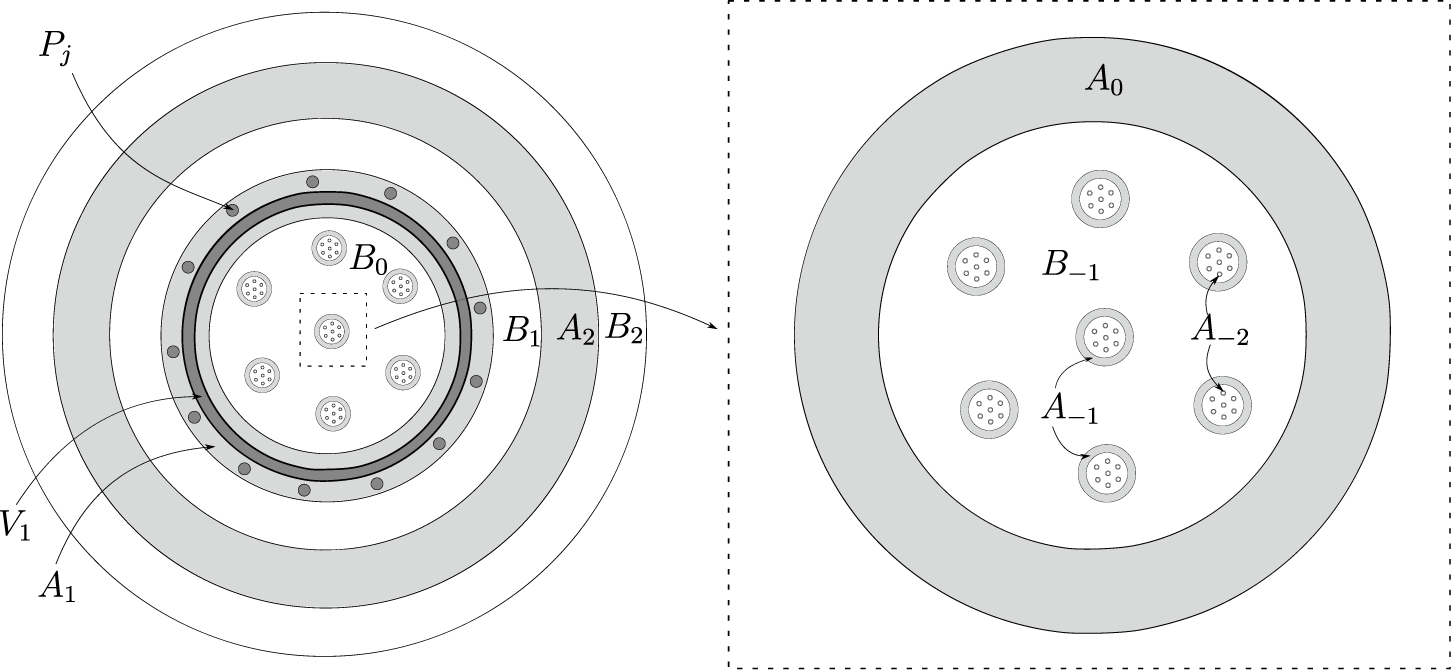
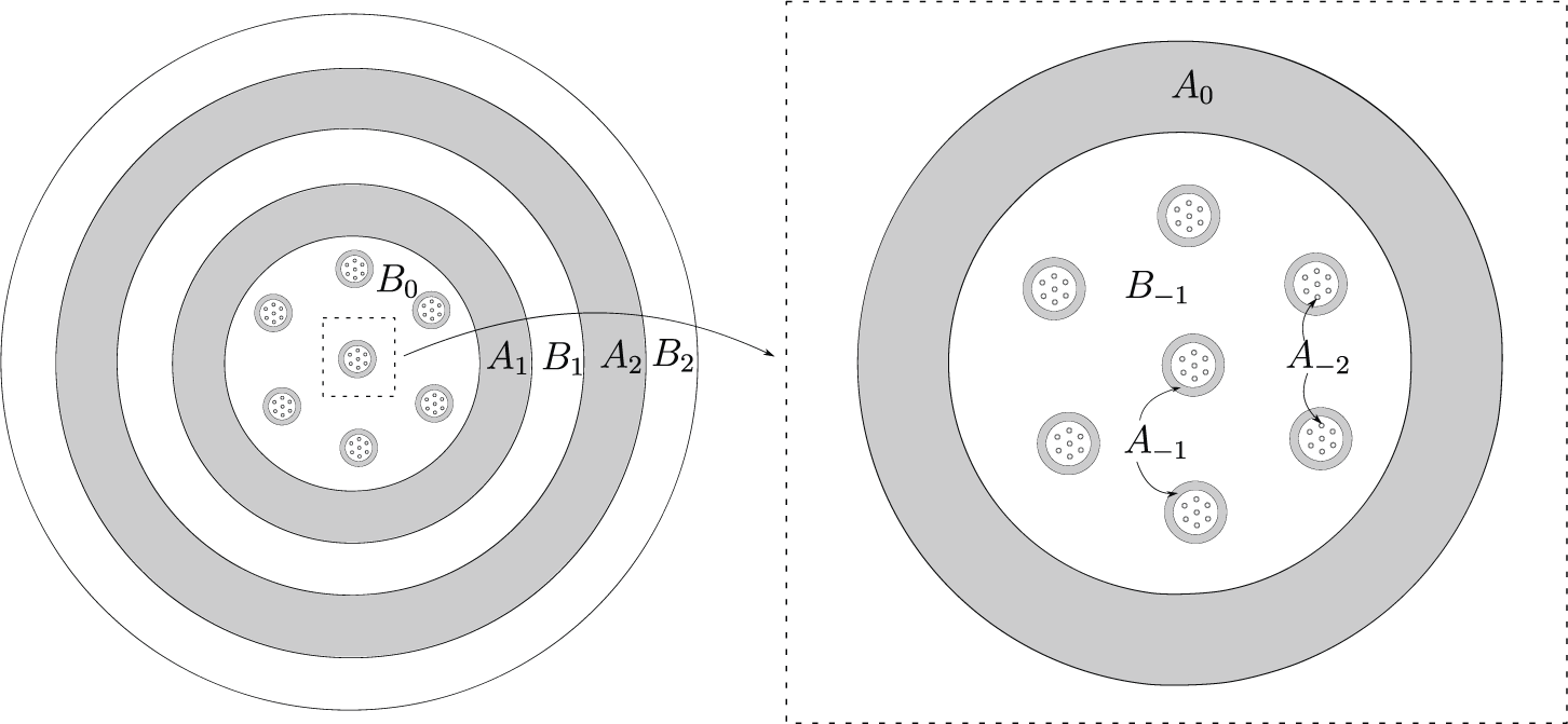
In §4, we define a sequence of annuli
 $A_k$
,
 $B_k$
for
 $k\geq 1$
(see Figure 2), and we prove the following mapping behavior. First, we show that
 $$ \begin{align*} f(B_k)\subset B_{k+1}. \end{align*} $$
Thus, each
 $B_k$
is contained in an m.c.w.d. of f. We define subannuli
 $V_k\subset A_k$
and prove that
 $$ \begin{align*} A_{k+1} \subset f(V_k). \end{align*} $$
We also prove in §6 that there are balls
 $P_j \subset A_k$
such that
 $P_j\cap V_k=\emptyset $
, which satisfy
 $$ \begin{align*} A_{k+1} \subset f(P_j), \end{align*} $$
and
 $f|_{P_j}$
is conformal.
Definition of
 $A_k$
,
 $B_k$
for all
 $k\in \mathbb {Z}$
. The annuli
 $A_k$
are shaded light gray and the
 $B_k$
are white. Also shown are
 $V_1\subset A_1$
and the ‘petals’
 $P_j\subset A_1$
(in dark gray).

The definition of the annuli
 $A_k$
,
 $B_k$
are extended to negative indices k by pulling back under f (see Figure 2). Together, the annuli
 $A_k$
and
 $B_k$
cover
 $\mathbb {C}$
except for a Cantor set, which we denote by E. This Cantor set E is the Julia set of the polynomial-like mapping obtained by restricting the definition of f to a subdomain of
 $\mathbb {C}$
, and we prove in §5 that
 $\text {dim}(E)\ll 1$
. Similarly, denoting by
 $E'$
the set of points that map to E, it is readily deduced that
 $\text {dim}(E')=\text {dim}(E)$
.
As the
 $B_k$
are contained in wandering components, we have that
 $$ \begin{align} \mathcal{J}(f)\setminus E' \subset \bigg\{ z \in\mathbb{C} : f^n(z) \in \bigcup_{k\in\mathbb{Z}} A_k \text{ for all } n \bigg\}. \end{align} $$
We denote the set defined on the right-hand side of equation (2.1) by X, so that estimating
 $\text {dim}(\mathcal {J}(f))$
reduces to estimating
 $\text {dim}(X)$
.
We partition X into two sets. For
 $z\in X$
, we say that z moves forwards if
 $z\in A_k$
and
 $f(z)\in A_{k+1}$
. If
 $z\in A_k$
and
 $f(z)\in A_j$
for
 $j\leq k$
, we say that z moves backwards. We denote by Y the set of
 $z\in X$
that move backwards infinitely often, and
 $Z:=X\setminus Y$
so that
 $$ \begin{align*} X = Y \sqcup Z. \end{align*} $$
In §8, we construct a sequence of covers
 $\mathcal {C}_m$
of Y, such that
 $\mathcal {C}_m$
covers all those points that move backwards m times. This is done by simply pulling back the annuli
 $A_k$
under iterates of f in regions where f is conformal. Standard distortion estimates apply when estimating the diameters of elements of
 $\mathcal {C}_m$
, and we deduce that
 $\text {dim}(Y)\ll 1$
.
The set Z is further partitioned into those points that eventually always stay in
 $\bigcup _k V_k$
, denoted by
 $Z_1$
, and
 $Z_2:=Z\setminus Z_1$
. The dimension of
 $\mathcal {J}(f)$
is supported on
 $Z_1$
. We prove in §9 that
 $Z_1$
consists of Jordan curves and we prove in §10 that these curves are in fact
 $C^1$
(hence, have dimension
 $1$
). We prove in §11 that
 $\text {dim}(Z_2)=0$
, and
 $Z_2$
is precisely the set of singleton complementary components in part (3) of Theorem 1.1.
3 Quasiconformal mapping estimates
In this section, we begin the proof of Theorem 1.1 by first applying Theorem A.17 (see Appendix A) to a specific sequence
 $(M_j)_{j=1}^\infty $
,
 $(r_j)_{j=1}^\infty $
that we now define. This yields an entire function f, so that
 $f\circ \phi =h$
is the quasiregular function described in §2. As discussed, we have freedom in describing the mapping behavior and dynamics of the quasiregular map h, but transferring this behavior to the entire function
 $f:=h\circ \phi ^{-1}$
requires estimates on
 $|\phi (z)-z|$
, and this is the main focus of this section.
Definition 3.1. We define an entire function f and a quasiconformal map
 $\phi : \mathbb {C}\rightarrow \mathbb {C}$
by applying Theorem A.17 to the parameters:
 $$ \begin{align} M_j:=2^{j}, r_1:=16, c_1:=1 \quad\text{and}\quad r_{j+1}:=c_{j}\cdot(\tfrac{1}{2}r_j)^{M_{j}} \quad\text{for } j\geq2. \end{align} $$
We will need some rough estimates on how fast
 $(r_j)_{j=1}^\infty $
grows and
 $(c_j)_{j=1}^\infty $
decays. We first show that by assuming
 $(r_j)_{j=1}^{\infty }$
satisfies some mild growth conditions, we can show that
 $(r_j^{M_j})_{j=1}^{\infty }$
grows much faster than
 $(c_j)_{j=1}^{\infty }$
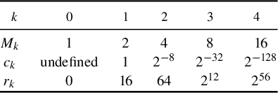
decays (see Table 1).
The values of
 $M_k$
,
 $c_k$
, and
 $r_k$
for small values of k. The sequence
 $M_k$
increases exponentially and
 $r_k$
increases super-exponentially, while
 $c_k$
decays super-exponentially.

Lemma 3.2. Assume for all
 $k \geq 3$
that
 $\sqrt {r_{k}} \geq r_j$
for all
 $j < k$
. Then, we have
 $$ \begin{align} r_k^{M_k} \cdot c_k = r_k^{M_k} \cdot \prod_{j=1}^{k-1} r_j^{-M_j} \geq r_k^{M_{k-1} + 1} \end{align} $$
for all
 $k \geq 3$
.
Proof. This is just a calculation, making use of the fact that
 $M_j - M_{j+1} = - M_j$
and
 $2M_{j} = M_{j+1}$
for all
 $j \geq 0$
, along with the definition of
 $c_k$
given by equation (A.15). When
 $k =1$
, we verify equation (3.2) by checking that
 $r_1^{M_1} = c_1 \cdot r_1^{M_0 + 1}$
. For the case of
 $k \geq 2$
, we verify equation (3.2) by computing
 $$ \begin{align*} r_k^{M_k} \cdot c_k &= r_k^{M_k} \cdot \prod_{j=2}^{k} r_{j-1}^{M_{j-1} -M_j} \\&= r_k^{M_k} \cdot \prod_{j=2}^{k} r_{j-1}^{-M_{j-1}} \\&\geq r_k^{M_k} \cdot \prod_{j=2}^{k} r_{k}^{-M_{j-2}} \quad (\sqrt{r_k} \geq r_j) \\&= r_k^{M_k} \cdot r_k^{-\sum_{j=0}^{k-2} M_j} \\&= r_k^{M_k - M_{k-1} + 1} = r_k^{M_{k-1} +1}. \end{align*} $$
In the last line, we used the fact that
 $\sum _{j=0}^{k-2} M_j = M_{k-1} -1$
.
Lemma 3.4. The sequence
 $(r_k)_{k=1}^{\infty }$
defined in Definition 3.1 satisfies:
-
(1)
$r_{2}> r_1$
; -
(2) for all
$k \geq 2$
,
$\sqrt {r_{k+1}} \geq r_k$
.


In particular,
 $(r_k)_{k=1}^{\infty }$
is an increasing sequence, and if
 $k \geq 2$
, we have
 $\sqrt {r_{k+1}} \geq r_j$
for all
 $j =1,\ldots ,k$
.
Proof. The claim
 $(1)$
is just a calculation:
 $$ \begin{align} r_2 = c_1\bigg(\frac{r_1}{2}\bigg)^{M_1} = 8^2 = 64> 16 = r_1. \end{align} $$
We will prove the second claim by induction. First, we have
 $$ \begin{align} r_3 = c_2\bigg(\frac{r_2}{2}\bigg)^{M_2} = 2^{-8}(2^5)^4= 2^{12} = 64^2. \end{align} $$
Therefore,
 $\sqrt {r_3} \geq r_2> r_1$
.
Suppose that for some
 $k \geq 3$
, we have
 $\sqrt {r_k} \geq r_{j}$
for all
 $j = 1,\ldots ,k-1$
. Then, by Lemma 3.2,
 $$ \begin{align} r_{k+1} = c_k r_k^{M_k} 2^{-M_k} \geq r_k^{M_{k-1} + 1} 2^{-M_k} = r_k^{M_{k-2} +1} r_k^{M_{k-2}} 16^{-M_{k-2}} \geq r_k^{M_{k-2}+1}. \end{align} $$
Since
 $k \geq 3$
, we have
 $M_{k-2} \geq M_1 = 2$
, so that
 $$ \begin{align} r_{k+1} \geq r_k \cdot r_k^2. \end{align} $$
Therefore, by the inductive hypothesis, we must have
 $\sqrt {r_{k+1}} \geq r_k \geq r_j$
for all
 ${j = 1,\ldots , k-1}$
. This proves the claim.
We record the following important inequalities that follow from the proof of Lemma 3.4.
Corollary 3.5. We have the following inequalities. For all
 $k \geq 3$
,
 $$ \begin{align} c_k r_k^{M_k} \geq r_k^{M_{k-1}+1} \quad\text{and}\quad \end{align} $$
 $$ \begin{align} r_{k+1} \geq 2^{-M_{k}} r_k^{M_{k-1}+1}.\ \ \end{align} $$
For all
 $k \geq 5$
, we have
 $$ \begin{align} r_{k+1} \geq 2^{2^{k}}= 2^{M_k} \quad\text{and}\quad \end{align} $$
 $$ \begin{align} r_{k+1} \geq 4 r_{k}^2. \end{align} $$
Proof. Most of the work has already been done in the proof of Lemma 3.4. We first prove equation (3.7). When
 $k \geq 2$
, By Lemma 3.4, we have
 $\sqrt {r_{k+1}} \geq r_j$
for all
 $j =1,\ldots k$
. Therefore, by Lemma 3.2, we obtain equation (3.7).
Equation (3.8) follows immediately. Indeed, the first two lines of equation (3.5) yields
 $$ \begin{align*}r_{k+1} \geq r_k^{M_{k-1}+1} 2^{-M_k},\end{align*} $$
when
 $k \geq 3$
.
When
 $k \geq 5$
, we can refine the estimate
 $r_{k+1} \geq r_k^{M_{k-2}+1}$
from equation (3.5). We note that by Lemma 3.4, we have
 $r_k> 16$
for all
 $k \geq 5$
. Therefore,
 $$ \begin{align*}r_{k+1} \geq r_k^{M_{k-2}+1}> 16^{M_{k-2}} = (2^4)^{M_{k-2}} = 2^{M_k}.\end{align*} $$
Finally, since
 $r_k> 16$
for all
 $k \geq 1$
, we certainly obtain equation (3.10) from equation (3.6).
Corollary 3.5 concludes our discussion of some technical relations and inequalities we will need for the sequences
 $(r_j)_{j=1}^\infty $
,
 $(c_j)_{j=1}^\infty $
. As discussed in §1, one of the key advantages of the quasiconformal approach (over the infinite-product approach) is the relative simplicity of deducing the singular value structure of the constructed function. This is summarized in the following proposition. Although equations (3.11) and (3.12) are slightly technical, they simply say the critical points are radially equidistributed on each circle
 $|z|=r_j$
, and the zeros are equidistributed on a slightly larger circle. Recall from Definition 3.1 that f is the entire function obtained by applying Theorem A.17 to the parameters in equation (3.1).
Proposition 3.6. Let
 $(M_j)_{j=1}^\infty $
,
 $(r_j)_{j=1}^\infty $
and
 $(c_j)_{j=1}^{\infty }$
be as in Definition 3.1. Then, the only critical points of f are
 $0$
and the simple critical points given by
 $$ \begin{align} \phi\bigg( r_j\cdot \exp\bigg(i\frac{(2k_j-1)\pi}{M_{j}} \bigg) \bigg), \end{align} $$
where
 $j\in \mathbb {N}$
and
 $1 \leq k_j \leq M_{j}$
. The only singular values of f are
 $0$
and the critical values
 $(\pm c_jr_j^{M_j})_{j=0}^\infty $
. The zeros of f are given by
 $$ \begin{align} 0\quad\text{and}\quad\phi\bigg( r_j \cdot \exp \bigg( \frac{1}{4}\frac{\pi}{M_{j}} + i \cdot \frac{(2k_j-1)\pi}{M_{j}} \bigg) \bigg), \end{align} $$
where
 $j \in \mathbb {N}$
and
 $1 \leq k_j \leq M_{j}$
. All of the zeros of f are simple except for
 $0$
that is of multiplicity
 $2$
.
Proof. This follows immediately from [Reference Burkart and LazebnikBL23, Proposition 3.21].
We now move on to show how to modify f near the origin so that instead of being modeled by a function of the form
 $z^n$
, it is modeled by a polynomial with a Cantor repeller Julia set. This will be advantageous because
 $z^n$
has a Julia set of dimension
 $1$
, whereas the constructed Cantor repeller will have dimension
 $\ll 1$
.
The main idea is that a monic, degree
 $M_k$
polynomial
 $p(z)$
behaves like
 $z\mapsto z^{M_k}$
near
 $\infty $
. We will show how to interpolate between
 $p(z)$
and
 $z\mapsto z^{M_k}$
in a way that is quasiconformal with dilatation bounded independent of k. Our strategy closely follows [Reference Fagella, Jarque and LazebnikFJL19, §3].
Definition 3.7. We define
 $$ \begin{align*} b(x)=\begin{cases} \exp\bigg(1+\dfrac{1}{x^2-1}\bigg) & \text{if } 0\leq x < 1, \\ 0 & \text{if } x\geq 1, \end{cases} \end{align*} $$
and, for
 $r\geq 1$
, the smooth map
 $$ \begin{align*} \widehat{\eta}_{r}(x)=\begin{cases} 1 & \text{if }x\leq r-1, \\ b(x-r+1) & \text{if } r-1 \leq x \leq r, \\ 0 & \text{if }x\geq r. \end{cases} \end{align*} $$
We also set
 $\eta _{r}(z)=\widehat {\eta }_{r}(|z|)$
.
Proposition 3.8. Let
 $g_k(z):=c_k z^{M_k}+ r_k z\eta _{r_k}(z)$
and
 $\mu _k:=(g_k)_{\overline {z}}/(g_k)_{z}$
. Then, there exists
 $K'\in \mathbb {N}$
with
 $K' \geq 5$
such that
 $$ \begin{align} \sup_{k\geq K'} \| \mu_k \|_{L^\infty(\mathbb{C})} < 1. \end{align} $$
Proof. We abbreviate
 $\eta (z):=\eta _{r_k}(z)$
. We use a similar strategy as in the proof of [Reference Fagella, Jarque and LazebnikFJL19, Lemma 3.1], and the initial steps of the proof are exactly the same. We have
 $$ \begin{align*} (g_k)_z(z)=M_kc_kz^{M_k-1}+r_k\eta(z)+r_kz\eta_z(z)\quad\text{and}\quad (g_k)_{\overline{z}}(z)=r_kz\eta_{\overline{z}}(z). \end{align*} $$
Solving
 $b"(x)=0$
, one sees that
 $|b'(x)|$
has a maximum at
 $x_0=(1/3)^{1/4}$
with
 $|b'(x_0)|<e$
, so that
 $|b'(x)|\leq e$
for
 $x\in [0,1]$
. Thus,
 $|(\widehat {\eta })'(x)|\leq e$
for all
 $x>0$
. Using the chain rule again, we have
 $$ \begin{align*} \bigg| \frac{\partial\eta}{\partial z}(z) \bigg| = | (\widehat{\eta})'(|z|) |\cdot\bigg| \frac{\partial|z|}{\partial z} \bigg| \leq \frac{e}{2}\quad \text{and} \quad \bigg| \frac{\partial\eta}{\partial \overline{z}}(z) \bigg| = | (\widehat{\eta})'(|z|) |\cdot\bigg| \frac{\partial|z|}{\partial \overline{z}} \bigg| \leq \frac{e}{2},\end{align*} $$
where we have used the fact that
 $$ \begin{align*}\frac{\partial|z|}{\partial z}=\frac{\overline{z}}{2|z|} \quad \text{and} \quad \frac{\partial|z|}{\partial \overline{z}}=\frac{z}{2|z|}.\end{align*} $$
Hence,
 $$ \begin{align} \bigg|\frac{(g_k)_{\overline{z}}(z)}{(g_k)_z(z)}\bigg| &\leq \frac{r_k|z|{e}/{2}}{| M_kc_k|z|^{M_k-1} - r_k|\eta(z)| - r_k|z|{e}/{2} | }\nonumber\\ &= \frac{{e}/{2}}{| {M_kc_k|z|^{M_k-2}}/{r_k} - {|\eta(z)|}/{|z|} - {e}/{2} | }. \end{align} $$
Let us consider the right-hand side of equation (3.14) for
 $|z|=r_k - 1$
, recalling
 $M_k:=2^k$
. We have that
 $$ \begin{align*} \frac{c_k|z|^{M_k-2}}{r_k}&:=\frac{1}{r_k(r_k-1)^2}\bigg(\prod_{j=2}^k\frac{1}{r_{j-1}^{M_j-M_{j-1}}}\bigg)(r_k-1)^{2^k} \\ &= \frac{1}{r_k(r_k-1)^2}\cdot\frac{(r_k-1)^2\cdot (r_k-1)^{2^2}\cdot\cdots\cdot (r_k-1)^{2^{k-1}}}{r_1^2\cdot r_2^{2^2}\cdot \cdots \cdot r_{k-1}^{2^{k-1}}} \\ &= \frac{(r_k-1)^{2^2}}{r_k} \cdot \frac{(r_k-1)^{2^3}}{r_1^2\cdot r_2^{2^2}\cdot r_3^{2^3}} \cdot \frac{(r_k-1)^{2^4}\cdot\cdots\cdot (r_k-1)^{2^{k-1}}}{r_4^{2^4} \cdot \cdots \cdot r_{k-1}^{2^{k-1}}}. \end{align*} $$
By Lemmas 3.4 and 3.5, we may deduce for all
 $k \geq 5$
,
 $$ \begin{align} r_k-1>2r_{k-1}, \end{align} $$
 $$ \begin{align} \frac{(r_k-1)^{2^3}}{r_1^2\cdot r_2^{2^2} \cdot r_3^{2^3}} \geq 1, \quad\text{and } \end{align} $$
 $$ \begin{align} (r_k-1)^2> r_k. \end{align} $$
Combining the above inequalities, it follows that when
 $|z| \geq r_k -1$
, we have
 $$ \begin{align} \frac{c_k|z|^{M_k-2}}{r_k} \geq r_{k-1}. \end{align} $$
Thus, it follows from equation (3.14) that in fact
 $|(g_k)_{\overline {z}}/(g_k)_z|\rightarrow 0$
as
 $k\rightarrow \infty $
.
Definition 3.9. Let f,
 $\phi $
be as in Definition 3.1, and
 $h:=f\circ \phi $
. We define a family of entire functions
 $f_N:=h_N\circ \phi _N^{-1}$
as follows. Let
 $$ \begin{align*} h_N(z):=\begin{cases} g_N(z) & \text{ if } |z|\leq r_N, \\ h(z) & \text{ if } |z|\geq r_N, \end{cases} \end{align*} $$
and
 $\phi _N: \mathbb {C}\rightarrow \mathbb {C}$
is the quasiconformal mapping such that:
-
(1)
$f_N$
is holomorphic; -
(2)
$\phi _N(0)=0$
; and -
(3)
$|\phi _N(z)/z - 1|\rightarrow 0$
as
$z\rightarrow \infty $
.


The fact that
 $\phi _N$
may be normalized so that condition (3) is satisfied follows from an argument similar to [Reference Burkart and LazebnikBL23].
Remark 3.10. We will always assume that
 $N \geq 5$
. Note that for
 $|z|=r_N$
, we have
 ${g_N(z)=h(z)}$
.
Remark 3.11. We will show that for all sufficiently large N, the function
 $f_N$
satisfies the conclusions of Theorem 1.1. We will occasionally omit the subscript N and simply write f when convenient.
Proposition 3.12. For
 $\phi _N$
as in Definition 3.9,
 $\sup _N K(\phi _N)<\infty $
.
Proof. By Proposition 3.8, we have
 $\sup _NK(\phi _N|_{\{|z|\leq r_N\}})<\infty $
and, by [Reference Burkart and LazebnikBL23, Proposition 4.6], we have
 $\sup _N K(\phi _N|_{\{|z|\geq r_N\}})<\infty $
.
In [Reference Burkart and LazebnikBL23], the conclusion
 $|\phi (z)/z-1|\xrightarrow {z\rightarrow \infty }0$
of Theorem A.17 is deduced by an application of the Teichmüller–Wittich–Belinskii theorem (see [Reference Lehto and VirtanenLV73, Theorem 6.1]). We will need a more quantitative statement for the purposes of proving Theorem 1.1, in particular, when we prove that the m.c.w.d.’s of Theorem 1.1 have smooth boundary. This quantitative statement is given in Theorem 3.14 below. The proof follows from the main arguments of [Reference ShishikuraShi18]. Indeed, Theorem 3.14 is quite analogous to the main result of [Reference ShishikuraShi18], but we will need to assume less than in [Reference ShishikuraShi18], and accordingly, we will obtain a weaker conclusion, which will nevertheless suffice to prove Theorem 1.1.
Definition 3.13. For
 $p\geq 1$
and
 $0 < r < 1$
, we will denote
 $$ \begin{align} \omega_p(r):=\big(\tfrac{1}{2}\big)^{p^{-1}\sqrt{\log\log r^{-1}}}.\end{align} $$
Theorem 3.14. Let
 $\psi : \mathbb {C} \rightarrow \mathbb {C}$
be a quasiconformal mapping,
 $\mu :=\psi _{\overline {z}}/\psi _z$
, and suppose that
 $$ \begin{align} I(r) := \int \!\!\!\!\int_{\{ |z|<r \}} \frac{|\mu|}{1-|\mu|^2} \frac{dx\,dy}{|z|^2} \text{ is finite and has order } O(\omega_1(r)) \text{ as } r\searrow0. \end{align} $$
Then,
 $\psi $
is conformal at
 $0$
and, for any
 $p>2$
, we have
 $$ \begin{align} \psi(z)=\psi(0)+\psi'(0)z+O(\omega_p(|z|)) \quad\text{as } z\rightarrow0. \end{align} $$
Proof. By [Reference ShishikuraShi18, Lemma 10], we have that for any
 $p>2$
and
 $0<\rho <1$
, there exists
 $C'=C'(p,\rho )$
such that if
 $0<|z_2|<\rho ^2|z_1|$
, then
 $$ \begin{align} &\bigg| \hspace{-3pt}\int \!\!\!\!\int_{\mathbb{C}} \frac{\mu(z)\phi_{z_1, z_2}(z)}{1-|\mu(z)|^2}\,dx\,dy \bigg|\nonumber\\ &\quad\leq \frac{1}{1-\rho^2}\bigg|\hspace{-3pt} \int\!\!\!\! \int_{A(\rho^{-1}|z_2|, \rho|z_1|)} \frac{\mu(z)}{1-|\mu(z)|^2}\frac{dx\,dy}{z^2} \bigg| +C'I_{p,2}(\mu; |z_1|)^{1/p},\end{align} $$
and
 $$ \begin{align} &\int \!\!\!\!\int_{\mathbb{C}} \frac{|\mu(z)|^2|\phi_{z_1, z_2}(z)|}{1-|\mu(z)|^2}\,dx\,dy\nonumber\\ &\quad \leq \frac{1}{1-\rho^2} \int\!\!\!\! \int_{A(\rho^{-1}|z_2|, \rho|z_1|)} \frac{|\mu(z)|^2}{1-|\mu(z)|^2}\frac{dx\,dy}{|z|^2} +C'I_{p,2}(\mu; |z_1|)^{1/p},\end{align} $$
where
 $$ \begin{align} \phi_{z_1, z_2}(z)=\frac{z_1}{z(z-z_1)(z-z_2)}\quad\text{and}\quad I_{p,2}:=\int \!\!\!\!\int_{\mathbb{C}} \frac{|\mu(z)|^p}{(1-|\mu(z)|^2)^p} \frac{dx\,dy}{|z|^2(1+|z|/r)^2}. \end{align} $$
Thus, by [Reference ShishikuraShi18, Theorem 8], it suffices to show that the
 $\liminf _{z_2\rightarrow 0}$
of the four terms on the right-hand sides of equations (3.22) and (3.23) are
 $O(\omega _p(|z_1|))$
as
 $z_1\rightarrow 0$
. In fact, we have better estimates on the two integral terms: they are
 $O(\omega _1(|z_1|))$
by assumption (3.20). For the remaining two terms, we use [Reference ShishikuraShi18, Lemma 11]: there exist constants
 $C_2$
and
 $C_3$
depending only on
 $K(\psi )$
such that for
 $0<r<r'$
,
 $$ \begin{align} I_{p,2}(\mu; r) \leq C_2 \int \!\!\!\!\int_{|z|<r'} \frac{|\mu(z)|^2}{1-|\mu(z)|^2}\frac{dx\,dy}{|z|^2} + \frac{C_3}{2}\bigg(\frac{r}{r'}\bigg)^2. \end{align} $$
Letting
 $r'=r^{1/2}$
, we see the first term on the right-hand side of equation (3.25) has order
 $O(\omega _1(r'))=O(\omega _1(r))$
, and the second term has order
 $O(r)$
, so that
 $I_{p,2}$
has order
 $O(\omega _1(r))$
. Thus,
 $I_{p,2}(\mu; |z_1|)^{1/p}$
has order
 $O(\omega _p(|z_1|))$
, and so the result follows.
Remark 3.15. One readily sees from the constants in the proof of Theorem 3.14 that the big-O constants in equation (3.21) depend only on
 $K(\psi )$
and the big-O constants in equation (3.20). In particular, they are independent of
 $N \in \mathbb {N}$
.
We now apply Theorem 3.14 to our particular setting.
Theorem 3.16. There exists
 $C'>0$
and
 $R>0$
such that for any
 $N\in \mathbb {N}$
and any
 $p>2$
,
 $$ \begin{align}\bigg|\frac{\phi_N(z)}{z} - 1\bigg| < C'\cdot\omega_p(1/|z|) \quad\text{for } |z|>R. \end{align} $$
Proof. Let
 $N\in \mathbb {N}$
. Let
 $\phi :=\phi _N: \mathbb {C}\rightarrow \mathbb {C}$
be a quasiconformal mapping such that
 ${h_{N}\circ \phi ^{-1}}$
is holomorphic and
 $\phi (0)=0$
. Consider
 $$ \begin{align*} \psi(z):=1/\phi(1/z), \end{align*} $$
and define
 $I(r)$
as in equation (3.20). We wish to apply Theorem 3.14. To this end, we calculate
 $$ \begin{align} I(r) \leq \frac{k}{1-k^2}\int\!\!\!\! \int_{(|z|<r)\cap\text{supp}(\psi_{\overline{z}})} \frac{dx\,dy}{|z|^2} \leq \frac{k}{1-k^2} \sum_{j\geq j(r)} \int\!\!\!\! \int_{G_j}\frac{dx\,dy}{|z|^2}, \end{align} $$
where
 $$ \begin{align} j(r) \text{ is the smallest integer such that } 1/r<r_{j(r)} \cdot \exp(\pi/M_j) \end{align} $$
and
 $$ \begin{align} G_j:=\{z\in\mathbb{C} : r_j^{-1} \cdot \exp(-\pi/M_j) \leq |z| \leq (r_j-1)^{-1} \}. \end{align} $$
As in the proof of [Reference Burkart and LazebnikBL23, Theorem 4.8], we calculate
 $$ \begin{align} \frac{k}{1-k^2} \sum_{j\geq j(r)} \int\!\!\!\! \int_{G_j}\frac{dx\,dy}{|z|^2} &\lesssim \sum_{j \geq j(r)} \int\!\!\!\! \int_{G_j}\frac{dx\,dy}{r_j^{-2}\exp(-2\pi/M_j)} \nonumber \\[-1pt]&= \sum_{j\geq j(r)} \frac{\pi((r_j-1)^{-2}-r_j^{-2}\exp(-2\pi/M_j))}{r_j^{-2}\exp(-2\pi/M_j)} \nonumber \\[-1pt]&\simeq \sum_{j \geq j(r)} \bigg(\bigg(\frac{r_j}{r_j-1}\bigg)^{2}\exp(2\pi/M_j)-1\bigg) \nonumber \\[-1pt]&\lesssim \sum_{j \geq j(r)} \bigg(\bigg(\frac{r_j}{r_j-1}\bigg)^{2}-1 + \bigg(\frac{r_j}{r_j-1}\bigg)^{2}\frac{4\pi}{M_j}\bigg) \nonumber \\[-1pt]&\lesssim \sum_{j \geq j(r)}\bigg( \frac{2r_j -1}{(r_j-1)^2} + \frac{8\pi}{M_j} \bigg) \nonumber \\[-1pt]&\lesssim \sum_{j \geq j(r)} \bigg( \frac{1}{r_j} + \frac{1}{M_j} \bigg) \nonumber\\[-1pt]&\lesssim \bigg(\frac{1}{2} \bigg)^{j(r)}, \end{align} $$
where we have used the fact that
 $M_j = 2^j$
, Corollary 3.5, and the inequality
 $$ \begin{align*}\exp(x) \leq 1 + 2x \quad\text{for all } x \leq 1.\end{align*} $$
Next, we note that
 $$ \begin{align} 2^{2^{(j+1)(j+2)/2}}>2^{2^{1+\cdots+j}+\cdots+2^j}>r_j \cdot \exp(\pi/M_j). \end{align} $$
Thus, it is readily calculated that
 $$ \begin{align} r_j \cdot \exp(\pi/M_j)> 1/r \implies (j+1)(j+2) > \log\log r^{-1}, \end{align} $$
and so since
 $(1/2)^j \simeq (1/2)^{\sqrt {(j+1)(j+2)}}$
, it follows that
 $$ \begin{align} r_j\cdot \exp(\pi/M_j)> \exp(-\pi/M_{j(r)})/r > 1/(2r) \implies \big(\tfrac{1}{2}\big)^j \lesssim \big(\tfrac{1}{2}\big)^{\sqrt{\log\log r^{-1}}}. \end{align} $$
Together, equations (3.27)–(3.33) imply that
 $I(r)$
is finite and has order
 $O(\omega _1(r))$
as
 $r\searrow 0$
, as needed. Thus, we may apply Theorem 3.14 to deduce that there exist
 $c>0$
and
 $r>0$
, so that
 $$ \begin{align} |\psi(z)/z-\psi'(0)| < c\cdot\omega_p(|z|) \quad\text{for } |z|<r. \end{align} $$
By multiplying
 $\psi $
by a complex constant, we may assume that
 $\psi '(0)=1$
. Since
 $1/\phi (1/z)=\psi (z)$
, the inequality (3.26) follows by taking
 $R=1/r$
and
 $C'>c$
. By Proposition 3.12 and Remark 3.15, the constants
 $C'$
and R do not depend on N since the above big-O estimates for
 $I(r)$
do not depend on N.
For the rest of the paper, we fix
 $C',R>0$
so that Theorem 3.16 holds.
Theorem 3.17. Let
 $\varepsilon>0$
. There exists
 $N_\varepsilon \in \mathbb {N}$
such that for
 $N>N_{\varepsilon }$
, we have
 $$ \begin{align}|\phi_N(z)-z| < \varepsilon \quad\text{for } |z|<R.\end{align} $$
Proof. Let
 $\mu _N$
be the Beltrami coefficient of
 $\phi _N$
. As
 $N\rightarrow \infty $
, we have
 $\mu _N\rightarrow 0$
pointwise. Thus, we have
 $|\phi _N(z)- z|\rightarrow 0$
uniformly on the compact set
 $|z|\leq R$
.
We conclude by restating Proposition 3.6 that listed the critical points and values of
 $f_N$
, but now adapted to account for the new behavior of the function
 $f_N$
near
 $0$
.
Lemma 3.18. Let
 $\{\zeta _j\}_{j=1}^{2^N-1}$
denote the
 $2^N-1$
many critical points of
 $g_{N}(z)$
contained in
 $B(0,r_N)$
. Then, the only critical points of
 $f_N$
are the simple critical points given by
 $\phi _N(\zeta _j)$
for
 $j =1,\ldots ,2^N-1$
, and the simple critical points given by
 $$ \begin{align} \phi_N\bigg( r_j\cdot \exp\bigg(i\frac{(2k_j-1)\pi}{M_{j}} \bigg) \bigg),\quad j \geq N, 1\leq k_j \leq M_j. \end{align} $$
The only singular values of
 $f_N$
are the critical values
 $(\pm c_j r_j^{M_j})_{j=N}^{\infty }$
and the critical values
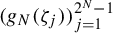 $(g_N(\zeta _j))_{j=1}^{2^N-1}$
.
4 Mapping behavior near
$\infty $

Having proven in §3 all the estimates on the ‘correction’ map
 $\phi $
that we will need, we can now begin describing the mapping behavior of the function
 $f:=h\circ \phi ^{-1}$
. In §4, we will introduce the annuli
 $A_k$
,
 $V_k$
,
 $B_k$
for
 $k\geq 1$
: these regions will be central to the proof of Theorem 1.1, as discussed in §2. We will also prove in Lemmas 4.17 and 4.18 the fundamental relations:
 $$ \begin{align*} f(B_k)\subset B_{k+1} \quad\text{and}\quad A_{k+1}\subset f(V_k) \quad\text{ for all } k\geq1. \end{align*} $$
In this section, and in the rest of the paper, we will consider the case
 $p = 2 \cdot \sqrt {2}$
for Definition 3.13. The following lemma gives us estimates for how
 $\omega _{2 \cdot \sqrt {2}}(|z|^{-1})$
decays as
 $z \rightarrow \infty $
.
Lemma 4.1. There exists
 $k_0\in \mathbb {Z}$
so that if
 $k \geq k_0$
and
 $|z| \geq {1}/{20} r_k$
, then
 $$ \begin{align} \omega_{2\sqrt{2}}\bigg(\frac{1}{|z|}\bigg) \leq \bigg( \frac{1}{2} \bigg)^{{\sqrt{k}}/{4}}. \end{align} $$
Proof. This is just a simple calculation using Definition 3.13 and Corollary 3.5. Indeed, for all
 $k \geq 10$
, we have
 $$ \begin{align*} \log \log \bigg(\frac{r_k}{20}\bigg ) &\geq \log \log \bigg(\frac{2^{M_{k-1}}}{20}\bigg) \\ &\geq \log \log (2^{M_{k-5}})\\ &= \log ( M_{k-5} \log 2) \\ &= \log (2^{k-5} \log 2) \\ &= (k-5) \log 2 + \log \log 2. \end{align*} $$
Therefore, there exists a value
 $k_0$
so that for all
 $k \geq k_0$
, we have
 $\log \log ({r_k}/{20}) \geq \tfrac 12k.$
For all such k, we verify that when
 $|z| \geq ({r_k}/{20})$
, we have
 $$ \begin{align*} \omega_{2\sqrt{2}}\bigg(\frac{1}{|z|} \bigg) & = \bigg(\frac{1}{2}\bigg)^{({1}/({2 \sqrt{2}}))\sqrt{\log\log |z|}} \leq \bigg(\frac{1}{2}\bigg)^{({1}/({2 \sqrt{2}}))\sqrt{\log\log ({r_k}/{20})}}\\ & \leq \bigg( \frac{1}{2} \bigg)^{({1}/({2 \sqrt{2}})) \sqrt{{k}/{2}}} = \bigg( \frac{1}{2} \bigg)^{{\sqrt{k}}/{4}}. \end{align*} $$
This yields equation (4.1) as desired.
Remark 4.2. Note that by perhaps choosing
 $k_0$
larger, we may additionally assume that
 $r_k \geq ({1}/{20})r_{k_0} \geq R$
for all
 $k \geq k_0$
. In this case, Theorem 3.16 and Lemma 4.1 imply that for all
 $k \geq k_0$
, if
 $|z| \geq ({r_k}/{20})$
, we have
 $({\phi _N(z)}/{z}) \in B(1,C' \cdot 2^{-\sqrt {k}/4}).$
Lemma 4.3. Let
 $k_0$
be as in Remark 4.2. For all
 $k \geq k_0$
, if
 $|z| \geq ({r_k}/{20})$
and
 $N \geq 5$
, we have
 $$ \begin{align} \big(1 - C' \cdot \big( \tfrac{1}{2} \big)^{{\sqrt{k}}/{4}}\big) |z| \leq |\phi_N(z)| \leq \big(1+ C' \cdot \big( \tfrac{1}{2} \big)^{{\sqrt{k}}/{4}}\big) |z|. \end{align} $$
Moreover, if
 $z \in \phi _N(\{w: |w| \geq ({r_k}/{20})\})$
, then
 $$ \begin{align} \frac{1}{\big(1+ C' \cdot \big( \tfrac{1}{2} \big)^{{\sqrt{k}}/{4}} \big)} |z| \leq |\phi_N^{-1}(z)| \leq \frac{1}{\big(1 - C' \cdot \big( \tfrac{1}{2} \big)^{{\sqrt{k}}/{4}} \big)} |z|. \end{align} $$
Proof. Equation (4.2) is just a rearrangement of equation (3.26), but using the estimate (4.1). For the second equation, just note that if
 $z \in \phi _N(\{w:|w| \geq ({r_k}/{20})\})$
, then there exists w with
 $|w| \geq ({r_k}/{20})$
so that
 $\phi _N(w) = z$
. Then, equation (4.2) holds with
 ${w = \phi _N^{-1}(z)}$
, so equation (4.3) is just a rearrangement of equation (4.2).
Remark 4.4. We will always assume that the integer
 $N \in \mathbb {N}$
satisfies
 $N \geq k_0$
.
Next, we will do some re-indexing of variables. This will make our notation easier to read and more consistent with [Reference BishopBis18].
Definition 4.5. Given the parameters
 $M_k$
,
 $c_k$
, and
 $r_k$
from Definition 3.1, and given any integer
 $N \geq 1$
, we define
 $$ \begin{align} n_k := M_{k+N-1} = 2^{N + k - 1}, \end{align} $$
 $$ \begin{align} R_k := r_{k+N-1}, \end{align} $$
and
 $$ \begin{align} C_k := c_{k+N-1}. \end{align} $$
Next, for any given
 $N \geq 1$
, we define
 $$ \begin{align} \alpha_k := \frac{1}{(1- C' \cdot ( {1}/{2} )^{({\sqrt{k+N-1}})/{4}})} \end{align} $$
and
 $$ \begin{align} \beta_k := \frac{1}{(1+ C' \cdot ( {1}/{2} )^{({\sqrt{k+N-1}})/{4}})}. \end{align} $$
Remark 4.6. As
 $k \rightarrow \infty $
, the sequence
 $(\alpha _k)$
decreases monotonically to
 $1$
, and
 $(\beta _k)$
increases monotonically to
 $1$
. We will always assume the integer
 $N \in \mathbb {N}$
is large enough so that for all
 $k \geq 1$
, we have
 $$ \begin{align} \frac{99}{100} < \beta_k < 1 < \alpha_k < \frac{101}{100}. \end{align} $$
The specific constants above are not important, we just need
 $\beta _k$
and
 $\alpha _k$
to be sufficiently close to
 $1$
for all large
 $k \geq 1$
.
Remark 4.7. We emphasize that the parameters in Definition 4.5 depend on
 $N \in \mathbb {N}$
; we omit this dependence in the notation for readability. We also remark that Definition 3.1 implies that we still have
 $R_{k+1} = C_{k} ({R_k}/{2})^{n_{k}}$
for all
 $k \geq 1$
. Finally, we have the equalities
 $R_1 = r_N$
and
 $n_1 = M_N$
. We will occasionally switch between the two forms of notation.
The inequalities (3.7), (3.8), (3.9), and (3.10) that apply to
 $(r_j)_{j=1}^{\infty }$
can now be restated as follows by applying Definition 4.5.
Lemma 4.8. Fix an integer
 $N \geq 5$
. Then, for all
 $k \geq 1$
, we have
 $$ \begin{align} R_k^{n_k} \cdot C_k \geq R_k^{n_{k-1}+1}, \end{align} $$
 $$ \begin{align} R_{k+1} \geq 2^{-n_{k}} \cdot R_k^{n_{k-1} +1}, \end{align} $$
 $$ \begin{align} R_k \geq 2^{2^{k + N -2}},\quad\text{and}, \end{align} $$
 $$ \begin{align} R_{k+1} \geq 4 R_k^2. \end{align} $$
The next lemma describes some relationships among the
 $n_k$
terms that we use freely throughout the paper.
Lemma 4.9. For all
 $k \geq 1$
, we have:
-
(1)
$2 n_k = n_{k+1}$
; -
(2)
$2^N + \sum _{j=1}^k n_j = n_{k+1}$
.


Proof. Part (1) is obvious. Part (2) is a simple calculation:
 $$ \begin{align*} 2^N + \sum_{j=1}^k n_j = 2^N\bigg(1+ \sum_{j=0}^{k-1} 2^j\bigg) = 2^N \cdot 2^k = 2^{N+k} = n_{k+1}. \end{align*} $$
This proves the claim.
We denote open round annuli centered at the origin by
 $A(r,R) = \{z: r < |z| < R\}$
. Next, we will define the following sequence of annuli. See Figures 2 and 3.
Definition 4.10. Given any
 $N \geq 1$
, we define
 $$ \begin{align} A_k = A\big(\tfrac{1}{4}R_k, 4 R_k\big), \quad B_k = \overline{A\big(4R_k, \tfrac{1}{4}R_{k+1}\big)},\quad V_k = A\big(\tfrac{2}{5}R_k, \tfrac{3}{5}R_k\big). \end{align} $$
A visualization of
 $A_k$
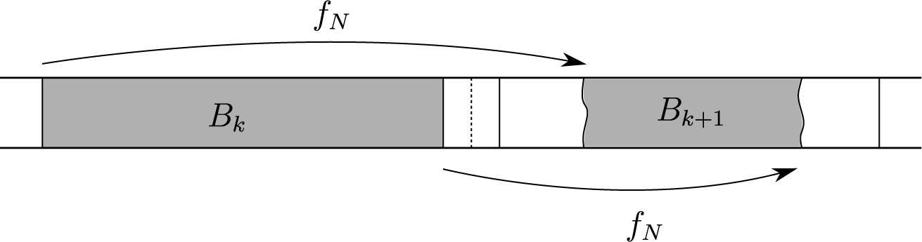
and
 $B_k$
viewed on the cylinder. The annuli
 $A_k$
have constant modulus, and the annulus
 $B_k$
have very large and increasing moduli.

We now begin to describe the mapping behavior of f in terms of the annuli in Definition 4.10.
Proposition 4.11. The zeros of
 $f_N$
that satisfy
 $|z| \geq \tfrac 14 R_1$
are contained in
 $\bigcup _{k=1}^{\infty } A_k$
. In fact, each
 $A_k$
contains exactly
 $n_{k}$
many simple zeros, each located inside
 $A(\tfrac 35 R_k, \tfrac 54 R_k)$
.

Lemma 4.12. There exists
 $M \in \mathbb {N}$
so that for all
 $N \geq M$
, for all
 $k \geq 1$
, and for all
 ${z \in A( \tfrac 54R_k, \tfrac 34 R_{k+1})}$
, we have
 $$ \begin{align} f_N(z) = C_{k+1} \cdot (\phi_N^{-1}(z))^{n_{k+1}}. \end{align} $$
Proof. If
 $z \in A(\exp ({\pi }/{n_{k}}) \cdot R_k, R_{k+1})$
, then
 $$ \begin{align*}f_N \circ \phi_N(z) = C_{k+1} \cdot z^{n_{k+1}}.\end{align*} $$
Therefore, if
 $z \in \phi _N (A(\exp ({\pi }/{n_{k}}) \cdot R_k, R_{k+1}))$
, we must have
 $$ \begin{align*}f_N(z) = C_{k+1} \cdot (\phi_N^{-1}(z))^{n_{k+1}}.\end{align*} $$
Therefore, it is sufficient to show that there is an M so that for all
 $N \geq M$
, and for all
 $k \geq 1$
, we have
 $$ \begin{align*}A\bigg( \frac{5}{4}R_k, \frac{3}{4} R_{k+1} \bigg) \subset \phi_N \bigg( A \bigg( \exp\bigg(\frac{\pi}{n_{k}}\bigg) \cdot R_k, R_{k+1}\bigg)\bigg).\end{align*} $$
The existence of such an M is a simple calculation using Lemma 4.3.
Lemma 4.13. There exists
 $M \in \mathbb {N}$
so that for all
 $N \geq M$
, for all
 $k\geq 1$
, and for all
 ${z \in A( \tfrac 54R_k, \tfrac 34 R_{k+1})}$
,
 $$ \begin{align} \beta^{n_{k+1}}_k C_{k+1}|z|^{n_{k+1}}\leq |f_N(z)| \leq \alpha^{n_{k+1}}_k C_{k+1} |z|^{n_{k+1}}. \end{align} $$
When estimating f near
 $|z| = R_1$
, we will require in some situations the following lemma, which is similar to Lemma 4.13. Recall that by Definition 3.9 for all
 ${z \in B(0, r_N - 1)}$
, we have
 $f_N(z) = q_N \circ \phi _N^{-1}(z)$
, where
 $q_N(z) = c_N z^{M_N} + r_N z = C_1 z^{n_1} + R_1 z.$
Lemma 4.14. There exists
 $M \in \mathbb {N}$
so that for all
 $N \geq M$
, we have
 $$ \begin{align} \frac{1}{2} c_N |z|^{M_N} \leq |q_N(z)| \leq 2 c_N |z|^{M_N} \quad\text{for all } z \in A\bigg(\frac{1}{20}R_1, \frac{19}{20}R_1\bigg). \end{align} $$
Proof. This is a simple but somewhat tedious application of Lemma 4.8. By the triangle inequality, we obtain for all
 $z \in A(({1}/{20})R_1, ({19}/{20})R_1)$
that
 $$ \begin{align*} c_N |z|^{M_N} \bigg(1 - \frac{r_N}{c_N |z|^{M_{N} - 1}}\bigg) \leq |q_N(z)| \leq c_N|z|^{M_N}\bigg( 1 + \frac{r_N}{c_N |z|^{M_N - 1}}\bigg). \end{align*} $$
On the one hand, we have by Lemma 3.5 that
 $$ \begin{align*} \max_{z \in A(({1}/{20})R_1, ({19}/{20})R_1)} \bigg( 1 + \frac{r_N}{c_N |z|^{M_N - 1}}\bigg) &= 1 + \frac{r_N}{c_N(({1}/{20})r_N)^{M_N - 1}} \\ &= 1 + \frac{r_N ({1}/{20})r_N}{({1}/{10})^{M_N} c_N({r_N}/{2})^{M_N}} \\ &= 1 + \frac{10^{M_N}}{20} \cdot \frac{r_N^{2}}{r_{N+1}} \\ &\leq 1 + \frac{10^{M_N}}{20} \cdot \frac{r_N^2}{2^{-M_N} r_N^{M_{(N-1)}}} \\ &\leq 1 + \frac{20^{M_N}}{20} \cdot \frac{1}{r_N^{M_{(N-2)}}} \\ &= 1 + \frac{1}{20} \bigg( \frac{20}{r_N^{{1}/{4}}} \bigg)^{M_N}. \end{align*} $$
By Lemma 4.8, there exists M so that for all
 $N \geq M$
, we have
 $r_N^{1/4} \geq 40$
and, therefore, we obtain
 $$ \begin{align*} \max_{z \in A(({1}/{20})R_1, ({19}/{20})R_1)} \bigg( 1 + \frac{r_N}{c_N |z|^{M_N - 1}}\bigg) \leq 1+\frac{1}{20} \cdot \bigg(\frac{1}{2}\bigg)^{M_N} < 2. \end{align*} $$
Therefore, we obtain for all
 $z \in z \in A(({1}/{20})R_1, ({19}/{20})R_1)$
that
 $$ \begin{align} |q_N(z)| \leq 2 c_N|z|^{M_N}. \end{align} $$
The proof of the other inequality is similar.
Lemma 4.15. For all N sufficiently large, we have
 $$ \begin{align} \frac{1}{2} \beta_1^{M_N} c_N |z|^{M_N} \leq |f_N(z)| \leq 2\alpha_1^{M_N} c_N |z|^{M_N} \quad\text{for all } z \in A\bigg(\frac{1}{10}R_1, \frac{9}{10}R_1\bigg). \end{align} $$
Proof. By Lemma 4.3, there exists
 $M \in \mathbb {N}$
so that for all
 $N \geq M$
, we have
 $$ \begin{align*} \phi^{-1}_N\bigg(A\bigg(\frac{1}{10}R_1, \frac{9}{10}R_1\bigg)\bigg) \subset A\bigg(\frac{1}{20}R_1, \frac{19}{20}R_1\bigg). \end{align*} $$
By perhaps choosing M larger, we have for all
 $N \geq M$
that
 $R_1 - 1 \geq ({19}/{20})R_1$
as well. Then, for all
 $z \in A(({1}/{10})R_1, ({9}/{10})R_1)$
, we have by Lemmas 4.3 and 4.14 that
 $$ \begin{align} \max_{z \in A(({1}/{10})R_1, ({9}/{10})R_1)} |f_N(z)| &= \max_{z \in A(({1}/{10})R_1, ({9}/{10})R_1)} |q_N(\phi_N^{-1}(z))|\nonumber\\ & \leq 2 c_N |\phi_N^{-1}(z)|^{M_N} \leq 2 c_N \alpha_1^{M_N} |z|^{M_N}. \end{align} $$
Similarly, we obtain
 $$ \begin{align} \min_{z \in A(({1}/{10})R_1, ({9}/{10})R_1)} |f_N(z)| &= \min_{z \in A(({1}/{10})R_1, ({9}/{10})R_1)} |q_N(\phi_N^{-1}(z))|\nonumber\\ & \geq \tfrac{1}{2} c_N |\phi_N^{-1}(z)|^{M_N} \geq \tfrac{1}{2} c_N \beta_1^{M_N}|z|^{M_N}. \end{align} $$
This proves the claim.
We are now ready to prove some basic lemmas about the macroscopic mapping behavior of the function
 $f_N$
. First, we will need the following basic lemma.
Lemma 4.16. Suppose that g is holomorphic on an annulus
 $W = A(a,b)$
and continuous up to the boundary of W. Let
 $U = A(c,d)$
.
-
(1) If
$|g(z)| \leq c$
on
$|z| = a$
and
$|g(z)| \geq d$
on
$|z| = b$
, then
$U \subset g(W)$
. -
(2) Suppose g has no zeros in W and that
$g(\partial W) \subset \overline {U}$
. Then,
$g(W) \subset \overline {U}$
.


Proof. The first part uses the fact that holomorphic maps are open. The second part is an application of the maximum principle. A detailed proof can be found in [Reference BishopBis18, Lemma 11.1].
Next, we prove the following lemma about the mapping behavior on
 $A_k$
, where we will see the dynamics of
 $f_N$
are the most interesting.
Lemma 4.17. There exists
 $M \in \mathbb {N}$
such that for all
 $N \geq M$
and for all
 $k \geq 1$
, we have
 $$ \begin{align} A_{k+1} \subset f_N(V_k) \subset f_N(A_k). \end{align} $$
Proof. First, we prove the case of
 $k \geq 2$
. In this setting, by Lemma 4.13,
 $$ \begin{align*} \max_{|z| = ({2}/{5})R_k} |f_N(z)| &\leq \max_{|z| = ({2}/{5})R_k} \alpha^{n_{k}}_k C_{k} |z|^{n_{k}} \leq \alpha^{n_{k}}_k C_k \big( \tfrac{2}{5} R_k \big)^{n_{k}} \leq \alpha^{n_{k}}_k \big( \tfrac{4}{5} \big)^{n_{k}} \cdot C_{k} \cdot \big(\tfrac{1}{2}R_k\big)^{n_{k}}. \end{align*} $$
By equation (4.9), we have
 $\alpha _k \cdot \tfrac 45 \leq \tfrac 78$
. Therefore, if
 $N \geq 5$
, since
 $R_{k+1}= C_{k} \cdot ({R_k}/{2})^{n_{k}}$
, we end up with
 $$ \begin{align} \max_{|z| = ({2}/{5})R_k} |f_N(z)| \leq \big(\tfrac{7}{8}\big)^{n_{k}} R_{k+1} < \tfrac{1}{4} R_{k+1}. \end{align} $$
Next, observe that by Lemma 4.13, we have
 $$ \begin{align*} \min_{|z| = ({3}/{5})R_k} \!|f_N(z)| \geq \min_{|z| = ({3}/{5})R_k} \!\beta_k^{n_k} C_k |z|^{n_{k}} = \beta_k^{n_k} C_k \big(\tfrac{3}{5} R_k\big)^{n_{k}} = \beta_k^{n_k} \cdot \big(\tfrac{6}{5}\big)^{n_k} \cdot C_{k} \cdot \big(\tfrac{1}{2}R_k\big)^{n_{k}}. \end{align*} $$
By equation (4.9), we have
 $\beta _k\cdot \tfrac 65 \geq \tfrac 98$
. If
 $N \geq 5$
, we end up with
 $$ \begin{align} \min_{|z| = ({3}/{5})R_k} |f_N(z)| \geq \big(\tfrac{9}{8}\big)^{n_{k}} R_{k+1}> 4 R_{k+1}. \end{align} $$
The lemma for the case of
 $k \geq 2$
now follows from Lemma 4.16, part
 $(1)$
.
The case of
 $k =1$
is almost exactly the same, except we now have to use Lemma 4.15. By following the exact same steps as above, we obtain since
 $N \geq 5$
that
 $$ \begin{align} \max_{|z| = ({2}/{5})R_1} |f_N(z)| \leq 2 \big(\tfrac{7}{8}\big)^{n_1}R_{2} < \tfrac{1}{4} R_2 \end{align} $$
and
 $$ \begin{align} \min_{|z| = ({3}/{5})R_1} |f_N(z)| \geq \tfrac{1}{2}\big(\tfrac{9}{8}\big)^{n_{1}} R_{2}> 4 R_2. \end{align} $$
The lemma for the case of
 $k = 1$
now follows from Lemma 4.16, part
 $(1)$
.
Lemma 4.18. There exists
 $M \in \mathbb {N}$
so that for all
 $N \geq M$
and for all
 $k \geq 1$
, we have
 $$ \begin{align} f_N(B_k) \subset B_{k+1}. \end{align} $$
Proof. We will adopt a similar strategy to Lemma 4.17, using Lemma 4.16, part
 $(2)$
. First, we make the important observation that
 ${C_{k+1}}/{C_k} = R_k^{-n_k}$
for all
 $k \geq 1$
. Next, observe that if
 $|z| = 4 R_k$
, then we have by Lemma 4.13,
 $$ \begin{align*} \max_{|z| = 4R_k} |f_N(z)| &\leq \max_{|z| = 4R_k} \alpha_k^{n_{k+1}} C_{k+1}|z|^{n_{k+1}} \\ &= \alpha_k^{n_{k+1}} C_{k+1} (4R_k)^{n_{k+1}} \\ &= \alpha_k^{n_{k+1}} 8^{n_{k+1}} \cdot C_{k} R_k^{-n_k}\cdot \big(\tfrac{1}{2}R_k\big)^{n_{k+1}} \\ &= \alpha_k^{n_{k+1}} 8^{n_{k+1}} C_{k} \big(\tfrac{1}{2}R_k\big)^{n_{k}} \cdot R_k^{-n_k} \big(\tfrac{1}{2}R_k\big)^{n_{k}}\\ &= \alpha_k^{n_{k+1}} 8^{n_{k+1}} 2^{-n_{k}} R_{k+1}. \\ &= (\alpha_k^2)^{n_{k}} 32^{n_{k}} R_{k+1}. \end{align*} $$
By equation (4.9), we have
 $\alpha _k^2 \leq 2$
for all
 $k \geq 1$
. By Lemma 4.8, there exists M so that for all
 $N \geq M$
, and for all
 $k \geq 1$
, we have
 $R_k^{1/2}> 256$
. Therefore,
 $$ \begin{align} \frac{64^{n_{k+1}} R_{k+1}}{R_{k+2}} \leq \frac{64^{n_{k+1}}R_{k+1}}{( {1}/{2})^{n_{k+1}} R_{k+1}^{n_k+1}} = \bigg(\frac{128}{R^{{1}/{2}}_{k+1}} \bigg)^{n_{k+1}} \leq \bigg(\frac{1}{2}\bigg)^{n_{k+1}}. \end{align} $$
By equation (4.28), and since
 $N \geq 5$
, we have for all
 $k \geq 1$
,
 $$ \begin{align} \max_{|z| = 4R_k} |f_N(z)| \leq 64^{n_{k+1}} R_{k+1} \leq \big( \tfrac{1}{2}\big)^{n_{k+1}} R_{k+2} < \tfrac{1}{8} R_{k+2}. \end{align} $$
Next, observe that by Lemma 4.13, we similarly have
 $$ \begin{align*} \min_{|z| = 4R_k} |f_N(z)| &\geq \min_{|z| = 4R_k} \beta_k^{n_{k+1}} C_{k+1}|z|^{n_{k+1}} \\ &= \beta_k^{n_{k+1}} C_k R_k^{-n_k} \cdot 2^{n_{k+1}} \bigg(\frac{R_k}{2}\bigg)^{n_{k}} \cdot \bigg(\frac{R_k}{2}\bigg)^{n_{k}} \\ &=(\beta^2_k)^{n_{k}} 2^{n_k} R_{k+1} = (2\beta_k^2)^{n_k} R_{k+1}. \end{align*} $$
By equation (4.9), we have
 $\beta _k^2 \cdot 2 \geq \tfrac 32$
. Therefore, since
 $N \geq 5$
, we have for all
 $k \geq 1$
that
 $$ \begin{align} \min_{|z| = 4R_k} |f_N(z)| \geq \big( \tfrac{3}{2} \big)^{n_{k}} R_{k+1}> 8 R_{k+1}. \end{align} $$
Therefore, by equations (4.29) and (4.30), for all
 $k \geq 1$
, we have
 $$ \begin{align} f_N(|z| = 4R_k) \subset A\big(8R_k,\tfrac{1}{8}R_{k+1}\big) \subset B_{k+1}. \end{align} $$
We can use similar techniques as above to analyze the behavior of
 $f_N$
on the outermost boundary of
 $B_k$
(see Figure 4). Indeed, we have
 $$ \begin{align} \max_{|z| = ({1}/{4})R_{k+1}} |f_N(z)| < \tfrac{1}{8} R_{k+2} \end{align} $$
and
 $$ \begin{align} \min_{|z| = ({1}/{4})R_{k+1}} |f_N(z)|> 8 R_{k+1}. \end{align} $$
Therefore, by equations (4.33) and (4.32), we have
 $$ \begin{align} f_N\big(|z| = \tfrac{1}{4} R_{k+1}\big) \subset A\big(8R_k,\tfrac{1}{8}R_{k+1}\big) \subset B_{k+1}. \end{align} $$
As we commented at the start, this proves the lemma.
We conclude this section by recording the location of the critical points and values of f in relation to the annuli
 $A_k$
,
 $B_k$
.
 $f_N$
maps the annulus
 $B_k$
into the annulus
 $B_{k+1}$
. The picture is not to scale; in reality, the modulus of
 $B_{k+1}$
is much larger than the modulus of
 $f_N(B_k)$
.

Proposition 4.19. There exists
 $M \in \mathbb {N}$
so that for all
 $N \geq M$
, all critical points z of
 $f_N$
with
 $|z|> \tfrac 14 R_1$
belong to
 $\bigcup _{k=1}^{\infty } A_k$
. Moreover, if
 $z \in A_k$
is a critical point, then
 ${f_N(z) \in B_{k+1}}$
.
Proof. By Proposition 3.6 and Lemma 4.3, there exists M so that for all
 $N \geq M$
, all critical points of
 $f_N$
satisfying
 $|z| \geq \tfrac 14 R_1$
belong to
 $\bigcup _{k=1}^{\infty } A_k$
. If
 $z \in A_k$
is a critical point, then Proposition 3.6 also says that
 $|f_N(z)| = C_k R_k^{n_k}$
. To see that
 $C_k R_k^{n_k} \in B_{k+1}$
, first notice that we have the identity
 $$ \begin{align} C_k R_k^{n_k} = 2^{n_k} C_k \big(\tfrac{1}{2}R_k\big)^{n_k} = 2^{n_k} R_{k+1}. \end{align} $$
It follows immediately from equation (4.35) that since
 $N \geq 5$
, we have
 $$ \begin{align} C_k R_k^{n_k} = 2^{n_k} R_{k+1}> 8R_{k+1}. \end{align} $$
However, we have by Lemma 4.8 that
 $$ \begin{align*} \frac{2^{n_k}R_{k+1}}{R_{k+2}} \leq \frac{8^{n_k}}{R_{k+1}^{n_k}} \leq \bigg(\frac{1}{2}\bigg)^{n_k}. \end{align*} $$
So since
 $N \geq 5$
, we obtain from equation (4.35) that
 $$ \begin{align} C_k R^{n_k}_k \leq \big( \tfrac{1}{2} \big)^{n_{k}} R_{k+2} < \tfrac{1}{8} R_{k+2}. \end{align} $$
Therefore, by equations (4.36) and (4.37), we have
 $f_N(z) \in B_{k+1}$
.
Remark 4.20. For the rest of the paper, we will always assume that N is large enough so that all of the statements and inequalities in this section are valid.
5 Mapping behavior near
$0$

Having studied the mapping behavior of f in the region
 $|z|>R_1/4$
in §4, we now study in §5 the mapping behavior of f in
 $|z|<R_1/4$
. Recall that in
 $|z|<R_1/4$
, the mapping f satisfies
 $f(z)=q_N\circ \phi _N^{-1}(z)$
, where
 $q_N(z) = c_N z^{M_N} + r_N z$
. This polynomial was chosen so as to have a Cantor Julia set of dimension
 $\ll 1$
. Thus, when we consider f as a polynomial-like mapping by restricting the domain of f to a subdomain of
 $|z|<R_1/4$
, we will see that the Julia set of this polynomial-like mapping has dimension
 $\ll 1$
.
We begin with the following lemma about the polynomial
 $q_N(z)$
.
Lemma 5.1. Let
 $q_N(z) = c_N z^{M_N} + r_N \cdot z$
. Then, the derivative of
 $q_N(z)$
is
 $$ \begin{align} q_N'(z) = c_N M_N z^{M_N-1} + r_N. \end{align} $$
The non-zeros of
 $q_N$
are given by
 $$ \begin{align} z = \bigg(\frac{-r_N}{c_N} \bigg)^{{1}/{M_N-1}}. \end{align} $$
The critical points of
 $q_N$
are given by
 $$ \begin{align} z = \bigg( \frac{-r_N}{c_N M_N}\bigg)^{{1}/{M_N-1}}. \end{align} $$
The critical values of
 $q_N$
lie on the circle
 $$ \begin{align} |z| = \bigg( \frac{r_N}{c_N M_N}\bigg)^{{1}/{M_N-1}} \cdot r_N \cdot \bigg(1- \frac{1}{M_N} \bigg). \end{align} $$
The value of
 $|q_N'(z)|$
when z is a zero of
 $q_N$
satisfies
 $$ \begin{align} |q_N'(z)| = r_N (M_N -1). \end{align} $$
Proof. These are all simple calculations. We only verify equation (5.4). If z is a critical point of
 $q_N$
, then we calculate that
 $$ \begin{align*} q_N(z) &= c_N \bigg( \frac{-r_N}{c_N M_N}\bigg)^{{M_N}/{M_N-1}} + r_N \bigg( \frac{-r_N}{c_N M_N}\bigg)^{{1}/{M_N-1}} \\ &= \bigg( \frac{-r_N}{c_N M_N}\bigg)^{{1}/{M_N-1}} \cdot \bigg(r_N - \frac{r_N}{M_N}\bigg) \\ &= \bigg( \frac{-r_N}{c_N M_N}\bigg)^{{1}/{M_N-1}} \cdot r_N \cdot \bigg( 1 - \frac{1}{M_N} \bigg). \end{align*} $$
The result follows upon taking the absolute value.
We will now prove that the critical values of
 $q_N$
map to
 $B_1$
. This will be crucial in dimension estimates that require coverings that are built by considering the inverse
 $f^{-1}$
. First, we need the following technical lemma.
Lemma 5.2. For all
 $N \geq 10$
, we have
 $$ \begin{align} 2^{M_{N-7}}r_{N-1} \leq \bigg( \frac{r_N}{c_N M_N} \bigg)^{{1}/{M_N - 1}} \leq \frac{1}{\sqrt{2}}r_{N-1}^2. \end{align} $$
Proof. Recall first that
 $r_N = c_{N-1} ({r_{N-1}}/{2})^{M_{N-1}}$
by definition. Therefore, we calculate
 $$ \begin{align} \frac{r_N}{c_N} = \frac{1}{2^{M_{(N-1)}}} \frac{c_{N-1} r^{M_{(N-1)}}_{N-1}}{c_N} = \frac{1}{2^{M_{(N-1)}}} \frac{r_{N-1}^{M_{(N-1)}}}{r_{N-1}^{-M_{(N-1)}}} = \frac{1}{2^{M_{(N-1)}}} r_{N-1}^{M_N}. \end{align} $$
First, we prove the upper bound for equation (5.6). First, note that we have for all
 $N \geq 5$
that
 $$ \begin{align} 2^{- {M_{(N-1)}}/{M_N - 1}} \leq \frac{1}{\sqrt{2}}, \end{align} $$
so that by combining equations (5.7) and (5.8), we obtain
 $$ \begin{align} \bigg( \frac{r_N}{c_N M_N} \bigg)^{{1}/{M_N - 1}} = \bigg(\frac{1}{M_N}\bigg)^{{1}/{M_N -1}} \cdot 2^{- {M_{(N-1)}}/{M_N - 1}} \cdot r_{N-1} \cdot r_{N-1}^{{1}/{M_N - 1}} \leq \frac{1}{\sqrt{2}} r_{N-1}^2. \end{align} $$
To prove the lower bound for equation (5.6), since
 $N \geq 5$
, note that we have
 $$ \begin{align} \bigg( \frac{1}{M_N} \bigg)^{{1}/{M_{N}-1}} \geq \frac{1}{2}\quad \text{and}\quad 2^{{-M_{N-1}}/{M_N -1}} \geq \frac{1}{2}. \end{align} $$
By two applications of Corollary 3.5, since
 $N \geq 10$
, we obtain
 $$ \begin{align} r_{N-1}^{{1}/{M_N-1}} \geq 2^{-{M_{(N-2)}}/{M_N -1}} \cdot r_{N-2}^{{M_{(N-3)}}/{M_N - 1}}\geq 2^{-1/2} r_{N-2}^{1/8} \geq 2^{-1/2} 2^{M_{N-3}/8} = 2^{M_{N-6} - 1/2}. \end{align} $$
Therefore, in a similar way to equation (5.9), except this time using equations (5.10) and (5.11), we have
 $$ \begin{align} \bigg( \frac{r_N}{c_N M_N} \bigg)^{{1}/{M_N - 1}} &= 2^{{-M_{(N-1)}}/{M_N -1}} \cdot \bigg(\frac{1}{M_N}\bigg)^{{1}/{M_N -1}} \cdot r_{N-1} \cdot r_{N-1}^{{1}/{M_N - 1}}\nonumber\\ &\geq 2^{M_{N-6} - 1/2 - 2} r_{N-1} \geq 2^{M_{N-7}} r_{N-1}. \end{align} $$
Lemma 5.3. For
 $N \geq 10$
, the critical values of
 $q_N$
belong to
 $B_1$
, and the critical points satisfy
 $|z| \leq r_{N-1}^2$
.
Proof. If z is a critical point, by Lemmas 5.1 and 5.2, we have
 $$ \begin{align} |z| = \bigg( \frac{r_N}{c_N M_N} \bigg)^{{1}/{M_N - 1}} \leq \frac{1}{\sqrt{2}}r_{N-1}^2. \end{align} $$
Recall that by Corollary 3.5 that if
 $N \geq 10$
, we have
 $r_{N-1}^2\leq \tfrac 14r_N$
and
 $r_N^2 \leq \tfrac 14r_{N+1}$
. So by Lemmas 5.1 and 5.2, if z is a critical point, then
 $$ \begin{align} |q_N(z)| = \bigg( \frac{r_N}{c_N M_N} \bigg)^{{1}/{M_N - 1}} r_N \bigg(1 - \frac{1}{M_N} \bigg) \leq \frac{1}{\sqrt{2}} r_{N-1}^2 r_N \leq \frac{1}{4\sqrt{2}} r_N^2 < \frac{1}{16\sqrt{2}} r_{N+1} \end{align} $$
and
 $$ \begin{align} |q_N(z)| \geq 2^{M_{(N-7)}} r_{N-1} r_N \cdot \bigg( 1 - \frac{1}{M_N} \bigg)> 8 r_N. \end{align} $$
Therefore, by Definition 4.5, we have the critical values of
 $q_N$
contained in
 $B_1$
, as desired.
Now we introduce a polynomial-like mapping by restricting f to a subdomain U, defined as follows.
Definition 5.4. For the rest of this section, we will use the following definitions.
-
(1) Define
$D = B(0, \tfrac 14R_1)$
. -
(2) Define
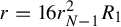
$r = 16 r_{N-1}^2 R_1$
. This is the same as
$r = 16r_{N-1}^2 r_N$
by equation (4.5). -
(3) Define
$V = B(0,r)$
and
$U' = q_N^{-1}(V)$
. -
(4) Define
$U = \phi _N(U')$
.



Lemma 5.5. For all
 $N \geq 10$
, the triple
 $q_N: U' \rightarrow V$
is a degree
 $2^N$
polynomial-like mapping. Moreover, all
 $2^{N} -1$
many critical points of
 $q_N$
belong to
 $U' \subset D$
.
Proof. We first verify that
 $U' \subset D$
. Note that if
 $|z| = \tfrac 14R_1 = \tfrac 14 r_N$
, then by Lemma 4.14, we have
 $$ \begin{align} |q_N(z)| &\geq \frac{1}{2} c_N \bigg( \frac{1}{4}r_N \bigg)^{M_N} \nonumber\\\nonumber &= \bigg( \frac{1}{2}\bigg)^{M_N + 1} r_{N+1} \\\nonumber &\geq \bigg( \frac{1}{4} \bigg)^{M_N+{1}/{2}} r_N^{M_{(N-1)}} r_N \quad (\text{Lemma~}4.8) \\&= \frac{1}{2} \bigg( \frac{r^{{1}/{4}}_N}{4} \bigg)^{M_N} r_N^{M_{(N-2)}} r_N. \end{align} $$
Therefore, since
 $N \geq 10$
, we have
 $r_N^{1/4}/4> 8$
and we deduce that
 $$ \begin{align} |q_N(z)| \geq 16 r_N^3> 16 r^2_{N-1}r_N. \end{align} $$
Therefore, we must have
 $U' \subset D$
.
By equation (5.14), the critical values of
 $q_N$
satisfy
 $|z| \leq r_{N-1}^2r_N$
. Therefore, V contains all
 $2^N-1$
many critical values of
 $q_N$
, so that
 $U'$
contains the
 $2^N - 1$
many critical points of
 $q_N$
. It now follows from Lemma A.11 that
 $q_N: U' \rightarrow V$
is a proper degree
 $2^N$
branched covering map, and it follows from Theorem A.13 that
 $U'$
is a Jordan domain. Since
 $U'$
is contained in D, which is compactly contained in V,
 $q_N: U' \rightarrow V$
is a degree
 $2^N$
polynomial-like mapping (see Figure 5).
Lemma 5.6. Let U be as in Definition 5.4 and
 $N \geq 10$
. Then,
 $U \subset D$
and the triple
 $f_N:U\rightarrow V$
is a degree
 $2^{N}$
polynomial-like mapping.
A schematic for Definition 5.4 and Lemma 5.5. The critical points for
 $q_N$
lie on the circle
 $|z| = ({r_N}/{c_NM_N})^{{1}/{M_N-1}}$
, and the associated critical values lie in an annulus contained in V, illustrated in gray. So, U contains the critical points of
 $q_N$
, and it will also be verified that
 $U \subset D$
.

Proof. By Lemma 4.3, we verify that
 $U = \phi _N(U') \subset D$
. Therefore, by Lemma 3.18,
 $f_N = q_N \circ \phi _N^{-1}: U \rightarrow V$
is a proper, degree
 $2^N$
branched covering map, and is therefore a degree
 $2^N$
polynomial-like mapping.
The rest of §5 is devoted to showing the filled Julia set of
 $f_N: U \rightarrow V$
has dimension
 $\ll 1$
. We will do so by constructing a cover by pulling back
 $B(0, 4R_1)$
under appropriate branches of
 $f^{-1}$
.
Remark 5.7. Suppose that
 $B(0,R)$
is the disk of radius R centered at the origin, where we take any
 $R \in [4R_1,8R_1]$
, so that
 $B(0,R) \subset V$
. By Lemmas 5.5 and 5.6,
 $\overline {B(0,R)}$
contains the
 $2^N-1$
many critical points of
 $f_N: U \rightarrow V$
. However, by equation (5.15),
 $B(0,R)$
does not contain the
 $2^N-1$
many critical values of
 $f_N: U \rightarrow V$
. It follows then from Lemma A.15 that
 $f_N^{-1}(B) \subset U$
is the disjoint union of
 $2^N$
many Jordan domains
 $B_i$
,
 $i=1,\ldots ,2^N$
such that
 $f_N: B_i \rightarrow B$
is conformal.
Remark 5.7 motivates the following definition (see Figure 6).
Definition 5.8. Define
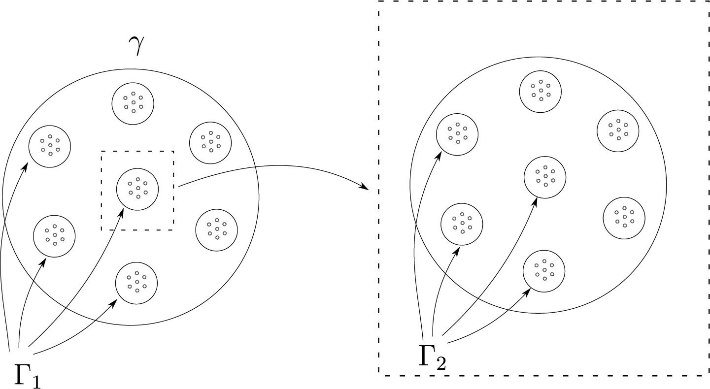
 $\gamma := \{z: |z| = 4R_1\}.$
Then,
 $\gamma $
is a circle that surrounds the critical points of
 $f_N$
contained in D, but not the critical values associated to those critical points.
-
(1) Let
$\Gamma _1 = f^{-1}_N(\gamma )$
be the disjoint union of the
$2^N$
many Jordan curves contained in D that
$f_N$
maps to
$\gamma $
. We denote the elements of
$\Gamma _1$
by
$\gamma _1$
. -
(2) Let
$\Gamma _n = f^{-n}_N(\gamma )$
be the disjoint union of
$2^{Nn}$
many Jordan curves in D that get mapped by
$f^n_N$
to
$\gamma $
. We denote the elements of
$\Gamma _N$
by
$\gamma _n$
. -
(3) Given
$\gamma _n \in \Gamma _n$
, we define
$\widehat {\gamma _n}$
to be the bounded simply connected domain with boundary given by
$\gamma _n$
. We define
$\widehat {\Gamma _n}$
to be the set of all
$\widehat {\gamma _n}.$


Remark 5.9. An alternative definition for
 $\gamma $
in Definition 5.8 would be
 $\sigma = \{z: |z| = 8R_1\}$
, and we analogously could define
 $\Sigma _n$
, elements
 $\sigma _n \subset \Sigma _n$
, and
 $\widehat {\sigma _n}$
. Then, for each
 $\sigma _n \in \Sigma _n$
,
 $\widehat {\sigma _n}$
contains exactly one element
 $\gamma _n \in \Gamma _n$
, and the modulus of
 $\widehat {\sigma _n} \setminus \overline {\widehat {\gamma _n}}$
is bounded below by
 $(2\pi )^{-1} \log 2> 0$
. For each
 $\sigma _n \in \Sigma _n$
, there exists some element
 $\sigma _{n-1} \in \Sigma _{n-1}$
such that
 $f_N: \widehat {\sigma _n} \rightarrow \widehat {\sigma _{n-1}}$
is conformal. This means that the corresponding mapping
 ${f_N: \widehat {\gamma _n} \rightarrow \widehat {\gamma _{n-1}}}$
is conformal, and by Remark A.7, Corollaries A.4 and A.6 apply with constants that do not depend on the integers N or n.
Illustration of Definition 5.8 of the families
 $\Gamma _n$
.

We now estimate the diameters of our covering of Definition 5.8.
Lemma 5.10. Let
 $\gamma $
,
 $\Gamma _n$
, and
 $\widehat {\Gamma _n}$
be as in Definition 5.8. Then, there exists a value
 $M \in \mathbb {N}$
so that for all
 $N \geq M$
, for all
 $n \geq 1$
, and for every
 $\gamma _n \in \Gamma _n$
, we have
 $$ \begin{align*}\operatorname{\mathrm{diameter}}(f_N(\gamma_n)) \geq R_1 \operatorname{\mathrm{diameter}}(\gamma_n).\end{align*} $$
Proof. Choose some
 $\widehat {\gamma _1} \in \widehat {\Gamma _1}$
, and let
 $z_0\in \widehat {\gamma _1}$
be a zero for
 $f_N$
. Such a
 $z_0$
exists since
 $f_N(\gamma _1) = \gamma $
surrounds the origin. Then, by Corollary A.6 and Remark 5.9 applied to the appropriate branch of the inverse
 $f^{-1}_N: B(0,4R_1) \rightarrow \widehat {\gamma _1}$
, there exists a constant
 $C>0$
such that
 $$ \begin{align*} \gamma_1 \subset B\bigg(z_0, \frac{C(4R_1)}{|f_N'(z_0)|}\bigg).\end{align*} $$
Therefore, by Theorem 3.17 and Lemma 5.1, there exists another constant
 $L>0$
so that
 $$ \begin{align*}\frac{\operatorname{\mathrm{diameter}}(f_N(\gamma_1))}{\operatorname{\mathrm{diameter}}(\gamma_1)} \kern1.5pt{\geq}\kern1.5pt \frac{1}{C} \cdot |f^{\prime}_N(z_0)| \kern1.5pt{=}\kern1.5pt \frac{1}{C} \cdot R_1(M_N \kern1.5pt{-}\kern1.5pt 1) \cdot|(\phi_N^{-1})'(z_0)| \geq \frac{R_1}{C}\kern1.5pt{\cdot}\kern1.5pt L \kern1.5pt{\cdot}\kern1.5pt (M_N\kern1.5pt{-}\kern1.5pt1).\end{align*} $$
This proves the estimate for the case of
 $n =1$
. For
 $n> 1$
, by Corollary A.4 and Remark 5.9, there exists a constant
 $c>1$
such that
 $$ \begin{align*}\frac{\operatorname{\mathrm{diameter}}(f_N(\gamma_n))}{\operatorname{\mathrm{diameter}}(\gamma_n)} &\geq \frac{1}{c} \frac{\operatorname{\mathrm{diameter}}(f_N^{n-1}(f_N(\gamma_n)))}{\operatorname{\mathrm{diameter}}(f_N^{n-1}(\gamma_n))}\\ &\geq \frac{1}{c} \frac{\operatorname{\mathrm{diameter}}(\gamma)}{\operatorname{\mathrm{diameter}}(\gamma_1)} \geq \frac{R_1}{c \cdot C} \cdot L \cdot (M_N-1).\end{align*} $$
Therefore, there exists
 $M \in \mathbb {N}$
so that for all
 $N \geq M$
and for all
 $n \geq 1$
, we have
 $$ \begin{align*}\frac{\operatorname{\mathrm{diameter}}(f_N(\gamma_n))}{\operatorname{\mathrm{diameter}}(\gamma_n)} \geq R_1.\end{align*} $$
This is exactly what we wanted to show.
Lemma 5.10 allows us to deduce the Hausdorff dimension of the Julia set of the polynomial-like mapping
 $f_N: U \rightarrow V$
.
Theorem 5.11. Let
 $t> 0$
be given. Then, there exists an integer M so that for all
 $N \geq M$
, the Hausdorff dimension of the filled Julia set of
 $f_N:U\rightarrow V$
is at most t.
Proof. For each
 $n \geq 1$
,
 $\widehat {\Gamma _n}$
is a covering of the Julia set of
 $(f_N,U,V)$
. Fix
 $t> 0$
. If
 ${\widehat {\gamma _n} \in \widehat {\Gamma _n}}$
, then
 $f_N(\widehat {\gamma _n}) =: \widehat {\gamma _{n-1}} \in \widehat {\Gamma _{n-1}}$
. Therefore, by Lemma 5.10, we have
 $$ \begin{align} \sum_{\widehat{\gamma_n} \in \widehat{\Gamma_n}} \operatorname{\mathrm{diameter}}(\widehat{\gamma_n})^t \leq R_1^{-t} \cdot 2^N \cdot \sum_{\widehat{\gamma_{n-1}} \in \widehat{\Gamma_{n-1}}} \operatorname{\mathrm{diameter}}(\widehat{\gamma_{n-1}})^t. \end{align} $$
It follows from equation (5.18) that
 $$ \begin{align} \sum_{n=1}^{\infty} \sum_{\widehat{\gamma_n} \in \widehat{\Gamma_n}} \operatorname{\mathrm{diameter}}(\widehat{\gamma_n})^t \leq \operatorname{\mathrm{diameter}}(\gamma)^t \cdot \sum_{n=1}^{\infty} 2^{Nn} R_1^{-tn}. \end{align} $$
The sum in equation (5.19) converges if and only if
 $$ \begin{align*}2^{N} R_1^{-t} < 1.\end{align*} $$
Therefore, we use Corollary 3.5 to see that
 $$ \begin{align} R_1^{-t} 2^N = r_N^{-t} 2^{N} \leq 2^{N-M_{N-1}t}. \end{align} $$
Choose M so that for all
 $N \geq M$
, we have
 $N - 2^{N-1}t < 0$
, so that we obtain
 $2^N R_1^{-t} < 1$
. For such a choice of N, equation (5.19) converges, and for any
 $\eta> 0$
, there exists some value n so that
 $$ \begin{align*}\sum_{\widehat{\gamma_n} \in \widehat{\Gamma_n}} \operatorname{\mathrm{diameter}}(\widehat{\gamma_n})^t < \eta.\end{align*} $$
Since
 $\widehat {\Gamma _n}$
is a covering of the filled Julia set of
 $f_N: U \rightarrow V$
, it follows that its Hausdorff dimension is bounded above by t.
We conclude §5 by showing that the critical values of
 $f_N$
lying in
 $|z|<R_1/4$
map to
 $B_1$
. This will be crucial in constructing covers of the Julia set of
 $f_N$
by pulling back the annuli
 $A_k$
under
 $f_N$
.
Lemma 5.12. For all
 $N \geq 10$
, if z is a critical point of
 $f_N$
contained in D, then
 ${f_N(z) \in B_1}$
.
Proof. The only critical points of
 $f_N$
contained inside of D are of the form
 $\phi _N(z)$
, where z is a critical point of
 $q_N$
. By Lemma 5.3, the critical values of
 $q_N$
are contained in
 $B_1$
. Therefore, the critical values of
 $f_N$
associated to the critical points in D belong to
 $B_1$
.
6 Location of the Julia set
In this section, we refine our understanding of the behavior of f in the annuli
 $A_k$
. Namely, we prove that unless z belongs to
 $V_k$
or a collection of small balls (which we call petals in Definition 6.2 below), then
 $f(z)\in B_{k+1}$
. This is crucial to our understanding of the structure of
 $\mathcal {J}(f)$
, since it is readily observed (see Lemma 6.1 below) that the annuli
 $B_k$
lie in
 $\mathcal {F}(f)$
. We will also further describe the behavior of f in the aforementioned petals.
Lemma 6.1. There exists
 $M \in \mathbb {N}$
such that for all
 $N \geq M$
,
 $B_k$
belongs to the Fatou set of
 $f_N$
for all
 $k \geq 1$
.
Proof. By Lemma 4.18, there exists
 $M \in \mathbb {N}$
such that for all
 $N \geq M$
, we have
 ${f_N(B_k) \subset B_{k+1}}$
. This implies that each point in
 $B_k$
escapes locally uniformly to
 $\infty $
.
Therefore, when
 $|z| \geq \tfrac 14 R_1$
, the Julia set of
 $f_N$
is contained in
 $\bigcup _{k=1}^{\infty } A_k$
. For each
 $k \geq 1$
, Proposition 4.11 says that
 $f_N$
has
 $n_k$
many zeros contained in
 $A_k$
. For a given
 $k \geq 1$
, let
 $\{w_j^k\}_{j=1}^{n_k}$
denote these zeros. Following the terminology in [Reference BishopBis18], we introduce some notation for the balls containing the zeros of
 $f_N$
inside of
 $A_k$
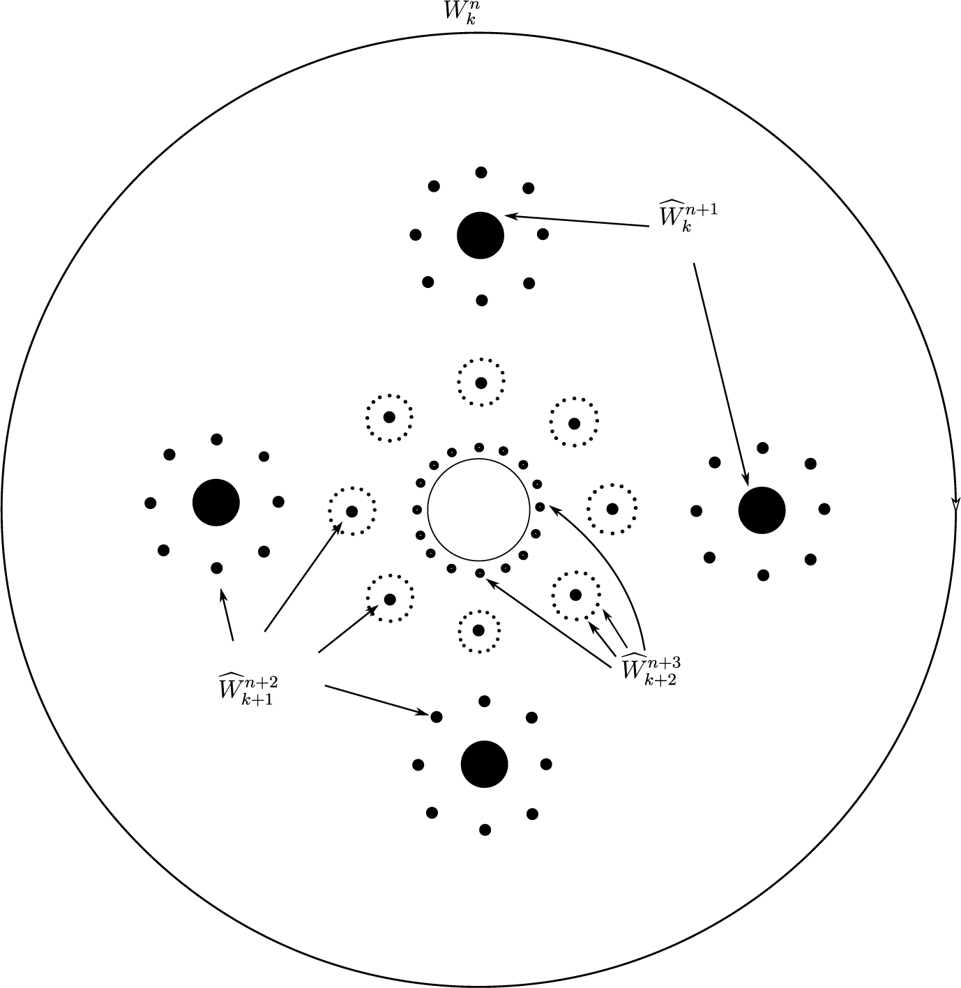
(see Figure 7).
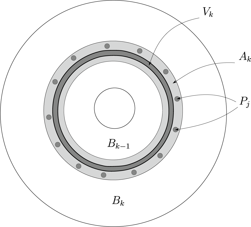
Definition 6.2. For
 $k \geq 1$
, let
 $\mathcal {P}_k = \bigcup _{j=1}^{n_k} B(w^k_j,R_k/2^{n_k})$
be the petals of
 $f_N$
inside of
 $A_k$
. A connected component
 $P_k \subset \mathcal {P}_k$
will be called a petal.
Illustration of Definition 6.2 of the petals
 $P_k$
. The annuli
 $B_{k-1}$
,
 $B_k$
are in white, the annulus
 $A_k$
is in light gray, and the annulus
 $V_k$
and petals
 $P_k$
are in dark gray.

As already mentioned, we will now prove several lemmas (Lemmas 6.3–6.8) detailing the mapping behavior of f within the annulus
 $A_k$
, most crucially within the subannulus
 $V_k$
and the petals
 $P_k$
.
Lemma 6.3. There exists
 $M \in \mathbb {N}$
so that for all
 $N \geq M$
, if
 $k \geq 1$
, then
 $$ \begin{align*}f_N\big(A\big(\tfrac{5}{4} R_k, 4 R_k\big)\big) \subset B_{k+1}.\end{align*} $$
Proof. By Proposition 4.11 and by Lemma 4.16, it is sufficient to verify that there exists
 $M \in \mathbb {N}$
so that for all
 $N \geq M$
, we have
 $f_N(|z| = 4R_k) \subset B_{k+1}$
and
 $f_N(|z| = \tfrac 54R_k) \subset B_{k+1}$
. The former has already been verified in equation (4.31), so we only need to prove the latter. By the maximum principle for holomorphic functions, we have
 $$ \begin{align} \max_{|z| = ({5}/{4})R_k} |f_N(z)| \leq \max_{|z| = 4R_k} |f_N(z)| < \tfrac{1}{8}R_{k+2}. \end{align} $$
By Lemma 4.13, we have
 $$ \begin{align*} \min_{|z| = ({5}/{4})R_k} |f_N(z)| &\geq \min_{|z| = ({5}/{4})R_k} C_{k+1} \beta_k^{n_{k+1}} |z|^{n_{k+1}} = \beta_k^{n_{k+1}} C_k \bigg( \frac{R_k}{2} \bigg)^{n_k} \bigg(\frac{5}{2}\bigg)^{n_{k+1}} \bigg(\frac{1}{2}\bigg)^{n_k}\\ & \geq \beta_k^{n_{k+1}} R_{k+1} \bigg(\frac{5}{4}\bigg)^{n_{k+1}}. \end{align*} $$
By equation (4.9), we have
 $\beta _k \cdot \tfrac 54\geq \tfrac 65$
. Therefore, since
 $N \geq 5$
, we have
 $$ \begin{align} \min_{|z| = ({5}/{4})R_k} |f_N(z)| \geq \big(\tfrac{6}{5}\big)^{n_{k+1}} R_{k+1}> 8R_{k+1}. \end{align} $$
It follows from equations (6.2) and (6.1) that
 $$ \begin{align} f_N\big(|z| = \tfrac{5}{4}R_k\big) \subset A\big(8R_{k+1}, \tfrac{1}{8}R_{k+2}\big) \subset B_{k+1}. \end{align} $$
As discussed at the beginning, this proves the claim.
Lemma 6.4. There exists
 $M \in \mathbb {N}$
so that for all
 $N \geq M$
, if
 $k \geq 1$
, then
 $$ \begin{align*} f_N\big(A\big(\tfrac{1}{4}R_k, \tfrac{2}{5}R_k\big)\big) \subset B_{k}. \end{align*} $$
Proof. We consider the cases of
 $k \geq 2$
and
 $k = 1$
separately.
When
 $k \geq 2$
, equation (4.34) implies that
 $f_N(|z| = \tfrac 14R_k) \subset B_{k}$
. By equation (4.23), we have
 $\max _{|z| = (2/5)R_k} |f_N(z)| \leq \tfrac 14R_{k+1}$
. Next, we observe that by Lemma 4.8,
 $$ \begin{align*} \min_{|z| = ({2}/{5})R_k} \!\!|f_N(z)| \geq\! \min_{|z| = ({2}/{5})R_k} \!\beta_k^{n_k} C_k |z|^{n_{k}} = \beta_k^{n_k} C_k \big(\tfrac{4}{5}\big)^{n_k} \big(\tfrac{1}{2}R_k\big)^{n_{k}} &= \beta_k^{n_k} R_{k+1} \big(\tfrac{4}{5}\big)^{n_k} \\&\geq \beta_k^{n_k} \big(\tfrac{4}{10}\big)^{n_k} R_k^{n_{k-1}} R_k. \end{align*} $$
Since
 $N \geq 5$
, by equation (4.9) and Lemma 4.8, we have
 $$ \begin{align} \beta_k \tfrac{4}{10} R^{{1}/{2}}_k \geq 4. \end{align} $$
Therefore, we obtain
 $$ \begin{align} \min_{|z| = ({2}/{5})R_k} |f_N(z)| \geq 4^{n_k} R_k> 8 R_k. \end{align} $$
It follows that
 $$ \begin{align} f_N\big(|z| = \tfrac{2}{5}R_k\big) \subset A\big(8R_{k}, \tfrac{1}{8}R_{k+1}\big) \subset B_k \end{align} $$
whenever
 $k \geq 2$
. Therefore, the case of
 $k \geq 2$
follows from part (2) of Lemma 4.16 and Proposition 4.11.
For the
 $k = 1$
case, we use slightly different estimates. First, notice that by following a similar argument as above, but applying Lemma 4.15, we obtain
 $$ \begin{align*} \min_{|z| = ({2}/{5})R_1} |f_N(z)| \geq \tfrac{1}{2} 4^{n_1} R_1> 8R_1. \end{align*} $$
This, combined with equation (4.25), allows us to conclude that
 $$ \begin{align} f_N\big(|z|= \tfrac{2}{5}R_1\big) \subset B_1. \end{align} $$
Next, by following similar reasoning as in equation (5.16), except this time applying Lemma 4.15, we have
 $$ \begin{align*} \min_{|z| = ({1}/{4})R_1} |f_N(z)| \geq \frac{1}{4} \beta_1^{M_N} \bigg( \frac{r_N^{{1}/{2}}}{4}\bigg)^{M_N} r_N^{M_{N-2}} r_N = \frac{1}{4}\bigg( \frac{\beta_1 r_N^{{1}/{2}}}{4}\bigg)^{M_N} r_N^{M_{N-2}} r_N. \end{align*} $$
By equation (4.9) and Lemma 4.8, along with similar reasoning as equation (5.17), we have
 $$ \begin{align} \min_{|z| = ({1}/{4})R_1} |f_N(z)|> 16 r^2_{N-1} r_N = 16 r^2_{N-1} R_1^2 > 4 R_1. \end{align} $$
So by equation (6.8) and the maximum principle used with equation (4.25), we have
 $$ \begin{align} f_N\big(|z| = \tfrac{1}{4}R_1\big) \subset B_1. \end{align} $$
The
 $k=1$
case now follows from Proposition 4.11 and part (2) of Lemma 4.16.
Lemma 6.5. There exists
 $M \in \mathbb {N}$
so that for all
 $N \geq M$
, if
 $k \geq 1$
, we have
 $$ \begin{align} f_N\big(|z| = \tfrac{3}{5}R_k\big) \subset B_{k+1}. \end{align} $$
Proof. We again must argue the
 $k=1$
and
 $k \geq 2$
cases separately.
When
 $k \geq 2$
, we have by Lemma 4.13 that
 $$ \begin{align*} \max_{|z| = ({3}/{5})R_k} |f_N(z)| &\leq \alpha_k^{n_k} C_k \big(\tfrac{3}{5}R_k \big)^{n_k} = \alpha_k^{n_k} C_k \big( \tfrac{6}{5} \big)^{n_k} \big( \tfrac{1}{2} R_k \big)^{n_k} = \alpha_k^{n_k} \big( \tfrac{6}{5} \big)^{n_k} R_{k+1}. \end{align*} $$
By equation (4.9), we have
 $\alpha _k \tfrac 65 \leq \tfrac 75$
. Therefore, since
 $N \geq 5$
, we obtain
 $$ \begin{align*} \frac{(\alpha_k ({6}/{5}))^{n_k}R_{k+1}}{R_{k+2}} \leq \frac{( {7}/{5})^{n_k}R_{k+1}}{2^{-n_{k+1}} R_{k+1}^{n_k + 1}} = \bigg( \frac{28}{5 R_{k+1}} \bigg)^{n_k} < \bigg(\frac{1}{4}\bigg)^{n_k}. \end{align*} $$
It follows that
 $$ \begin{align} \max_{|z| = ({3}/{5})R_k} |f_N(z)| \leq \big(\tfrac{1}{4}\big)^{n_k} R_{k+2} < \tfrac{1}{8}R_{k+2}. \end{align} $$
Therefore, we have by equations (4.24) and (6.11) that
 $$ \begin{align} f_N\big(|z| = \tfrac{3}{5}R_k\big)\subset A\big(8R_{k+1}, \tfrac{1}{8}R_{k+2}\big) \subset B_{k+1}. \end{align} $$
For the
 $k = 1$
case, the arguments are similar, and by using Lemma 4.15 and requiring
 $N \geq 5$
, we obtain
 $$ \begin{align} \max_{|z| = ({3}/{5})R_1} \leq 2 \big( \tfrac{1}{4} \big)^{n_k} R_{3} < \tfrac{1}{8} R_3. \end{align} $$
Therefore, by equations (4.26) and (6.13), we obtain
 $$ \begin{align} f_N\big(|z| = \tfrac{3}{5}R_1\big) \subset A\big(8R_2,\tfrac{1}{8}R_3\big) \subset B_{3}. \end{align} $$
Corollary 6.6. For all
 $k \geq 1$
, we have
 $f_N(V_k) \subset B_k \cup A_{k+1} \cup B_{k+1}$
.
Proof. By equations (6.6) and (6.7), along with equations (6.12) and (6.14), we have
 $f_N(|z|=\tfrac 25R_k) \subset B_k$
and
 $f_N(|z| = \tfrac 35R_k) \subset B_{k+1}$
for all
 $k \geq 1$
. Therefore, by part (2) of Lemma 4.16, we have
 $f_N(V_k) \subset B_k \cup A_{k+1} \cup B_{k+1}$
, as desired.
The following lemma asserts that
 $f_N$
is conformal on every petal
 $P_k \subset \mathcal {P}_k$
, with large expansion.
Lemma 6.7. There exists an
 $M \in \mathbb {N}$
and a constant
 $\unicode{x3bb}> 0$
so that for all
 $N \geq M$
, for all
 $k \geq 1$
, and for all zeros
 $w_j^k$
in
 $A_k$
,
 $j = 1,\ldots ,n_k$
, the mapping
 $$ \begin{align} f_N: B(w^k_j, \unicode{x3bb} ( \exp(\pi/n_k) - 1 ) R_k) \rightarrow f_N(B(w^k_j, \unicode{x3bb} ( \exp(\pi/n_k) - 1 ) R_k)) \end{align} $$
is conformal. Moreover, we have
 $$ \begin{align} B\bigg(w_j^k, \frac{R_k}{2^{n_k}}\bigg) \subset B(w^k_j, \unicode{x3bb} ( \exp(\pi/n_k) - 1 ) R_k) \end{align} $$
and
 $$ \begin{align} B(0,4 R_{k+1}) \subset f_N\bigg(B\bigg(w^k_j, \frac{R_k}{2^{n_k}}\bigg)\bigg). \end{align} $$
Proof. Note that by Lemmas A.19 and 4.3, there exist constants
 $\unicode{x3bb}>0$
and
 $\delta>0$
so that
 $$ \begin{align} B(0, \delta C_k R_k^{n_k}) \subset f_N(B(w^k_j, \unicode{x3bb} ( \exp(\pi/n_k) - 1 ) R_k)) \subset B\big(0, \tfrac{1}{2} C_kR_k^{n_k}\big). \end{align} $$
Moreover, Lemmas A.19 and 4.3 imply that the mapping in equation (6.15) is injective, and therefore conformal. Next, note that
 $$ \begin{align} \frac{2^{-n_k} R_k}{\unicode{x3bb}(\exp(\pi/n_k)-1)R_k} \leq \frac{2^{-n_k}}{\unicode{x3bb}\pi / n_k} = \frac{n_k}{2^{n_k} \pi \unicode{x3bb}} \xrightarrow[]{k \rightarrow \infty} 0. \end{align} $$
Therefore, there exists M so that for all
 $N \geq M$
, we have equation (6.15) and
 $B(w_j^k, R_k/2^{n_k}) \subset B(w^k_j, \unicode{x3bb} ( \exp (\pi /n_k) - 1 ) R_k)$
. It remains to verify that equation (6.17) holds.
To see this, note that by Theorem A.1 and equation (6.18), we have
 $$ \begin{align*} |(f_N)'(w^k_j)| &\geq \frac{1}{4} \frac{\operatorname{\mathrm{dist}}(0, \partial B(0,\delta C_k R_k^{n_k}))}{\operatorname{\mathrm{dist}}(w^k_j,\partial B(w^k_j, \unicode{x3bb} ( \exp(\pi/n_k) - 1 ) R_k) ))} \\ &= \frac{\delta }{4 \unicode{x3bb}} \frac{C_kR_k^{n_k}}{(\exp(\pi/n_k) - 1 )R_k} \\ &\geq \frac{\delta}{8 \unicode{x3bb} \pi} n_k C_k R_k^{n_k - 1} \\ &= \frac{\delta}{8 \unicode{x3bb} \pi} 2^{n_k} n_k R_{k+1} R_k^{-1}. \end{align*} $$
Therefore, if
 $w^k_j$
is a zero of
 $f_N$
in
 $A_k$
, we have
 $$ \begin{align} |(f_N)'(w^k_j)| \geq \frac{\delta}{8 \unicode{x3bb} \pi} 2^{n_k} n_k R_{k+1} R_k^{-1}. \end{align} $$
Next, consider the branch of the inverse
 $f_N^{-1}: B(0,\delta C_k R_k^{n_k}) \rightarrow D'$
, where
 $$ \begin{align*}D' \subset B(w^k_j, \unicode{x3bb} ( \exp(\pi/n_k) - 1 ) R_k).\end{align*} $$
Since
 $\delta>0$
is fixed, there exists a perhaps larger
 $M \in \mathbb {N}$
so that for all
 $N \geq M$
, we have
 $\delta 2^{n_1}> 4$
. Therefore,
 $$ \begin{align} \delta C_k R_k^{n_k} = \delta 2^{n_k} C_k\big(\tfrac{1}{2}R_k\big)^{n_k} = \delta 2^{n_k} R_{k+1}> 2^{n_{k-1}} 4R_{k+1} > 4R_{k+1}. \end{align} $$
We can further deduce from equation (6.21) that the modulus of the annulus
 $B(0,\delta C_k R_k^{n_k}) \setminus \overline {B(0,4R_{k+1})}$
is bounded below by some fixed constant independent of k. Denote
 $D = f_N^{-1}(B(0,4R_{k+1})) \subset D'$
. By applying Corollary A.6 to
 ${f_N^{-1}: B(0,4R_{k+1}) \rightarrow D}$
, we see that there exists a constant
 $L'>0$
such that
 $$ \begin{align} \frac{4R_{k+1}}{L'} \frac{1}{|f'(w^k_j)|} \leq r_{D,w^k_j} \leq R_{D,w^k_j} \leq L' \frac{4R_{k+1}}{|f'(w^k_j)|}. \end{align} $$
Since the modulus of
 $B(0,\delta C_k R_k^{n_k}) \setminus \overline {B(0,4R_{k+1})}$
is bounded below by some fixed constant independent of k, the constant
 $L'$
is independent of k and
 $w^k_j$
. By perhaps increasing M, we have that for all
 $N\geq M$
,
 $$ \begin{align} 4 R_{k+1}L' |f'(w_j^k)|^{-1} \leq 4 R_{k+1}L'\frac{8 \unicode{x3bb} \pi}{\delta n_k} 2^{-n_k} R^{-1}_{k+1} R_k \leq \frac{R_k}{2^{n_k}}. \end{align} $$
Therefore, by equations (6.22) and (6.23), and equation (A.6), we have
 $$ \begin{align*}D \subset B\bigg(w_j^k, L'\frac{4R_{k+1}}{|f'(w_j^k)|}\bigg) \subset B\bigg(w_j^k,\frac{R_k}{2^{n_k}}\bigg).\end{align*} $$
This proves equation (6.17), which is exactly what we wanted to show.
Lemma 6.8. For all
 $k \geq 1$
,
 $f_N(A(\tfrac 35R_k, \tfrac 54R_k) \setminus \overline {\bigcup _{j=1}^{n_k}B(w^k_j, R_k/2^{n_k})}) \subset B_{k+1}$
.
Proof. First, observe that every connected component of the boundary of
 $A(\tfrac 35R_k, \tfrac 54R_k) \setminus \overline {\bigcup _{j=1}^{n_k} B(w^k_j, R_k/2^{n_k})}$
is mapped inside of
 $B_{k+1}$
by
 $f_N$
. Indeed, by Lemma 6.5,
 $f_N(|z| = \tfrac 35R_k) \subset B_{k+1}$
, and by equation (6.3),
 $f_N(|z| = \tfrac 54 R_k) \subset B_{k+1}$
. The rest of the connected components of the boundary of
 $A(\tfrac 35R_k, \tfrac 54R_k) \setminus \overline {\bigcup _{j=1}^{n_k} (w^k_j, R_k/2^{n_k})}$
are the boundaries of the petals
 $P_k \subset \mathcal {P}_k$
. By equation (6.17),
 $$ \begin{align} f_N\bigg(\partial B\bigg(w_j^k, \frac{R_k}{2^{n_k}}\bigg)\bigg) \subset \{|z| \geq 4 R_{k+1}\}. \end{align} $$
By equations (4.37) and (6.18), we have
 $$ \begin{align} f_N\bigg(\partial B\bigg(w_j^k, \frac{R_k}{2^{n_k}}\bigg)\bigg) \subset B\bigg(0, \frac{1}{2}C_kR_k^{n_k}\bigg) \subset B\bigg(0, \frac{1}{4}R_{k+2}\bigg). \end{align} $$
Equations (6.24) and (6.25) imply
 $$ \begin{align} f_N\bigg(\partial B\bigg(w_j^k, \frac{R_k}{2^{n_k}}\bigg)\bigg) \subset B_{k+1}. \end{align} $$
By Proposition 4.11,
 $f_N$
has no additional zeros in
 $A(\tfrac 35R_k, \tfrac 54R_k) \setminus \overline {\bigcup _{j=1}^{n_k} B(w^k_j, R_k/2^{n_k})}$
. The result now follows from the maximum principle and minimum principle for non-zero holomorphic functions.
With Lemmas 6.3–6.8 in hand, we can now deduce the following about the Julia set of
 $f_N$
.
Theorem 6.9. There exists
 $M \in \mathbb {N}$
so that if
 $N \geq M$
, then for all
 $k \geq 1$
,
 $$ \begin{align*}(\mathcal{J}(f_N) \cap A_k) \subset \bigg( \bigcup_{j=1}^{n_k} B\bigg(w^k_j,\frac{R_k}{2^{n_k}}\bigg)\bigg) \cup V_k.\end{align*} $$
Proof. We will show that all other points get mapped to
 $B_k$
or
 $B_{k+1}$
, so that they belong to the Fatou set of
 $f_N$
by Lemma 6.1. Suppose that
 $z \in A_k \cap \mathcal {J}(f_N)$
, but
 $z \notin \mathcal {P}_k$
. Then, by Lemma 6.3,
 $z \notin A(\tfrac 54R_k, 4 R_k)$
, and by Lemma 6.4,
 $z \notin A(\tfrac 14R_k, \tfrac 25 R_k)$
. Similarly, Lemma 6.8 and the assumption that
 $z \notin \mathcal {P}_k$
shows that
 $z \notin A(\tfrac 35R_k, \tfrac 54R_k)$
. Finally, observe that we cannot have
 $z \in \{|z| = \tfrac 25R_k\}$
,
 $z \in \{|z| = \tfrac 35R_k\}$
, or
 $z \in \{|z| = \tfrac 54 R_k\}$
by equations (6.6) and (6.7), (6.10), and (6.3), respectively. Since
 $z \in A_k \cap J(f_N)$
, but
 $z \notin \mathcal {P}_k$
, it follows that
 $z \in A(\tfrac 25R_k, \tfrac 35R_k) = V_k$
, which proves the theorem.
The same argument of the proof of Theorem 6.9 yields the following useful result.
Lemma 6.10. Suppose that
 $z \in A_k$
and
 $f_N(z) \in A_{j}$
for some
 $k \geq 1$
and some
 $j \in \mathbb {Z}$
. Then,
 $$ \begin{align*}z \in V_k \cup \bigg( \bigcup_{j=1}^{n_k} B\bigg(w^k_j,\frac{R_k}{2^{n_k}}\bigg)\bigg).\end{align*} $$
7 Conformal mapping behavior
We begin §7 by defining
 $A_k$
,
 $B_k$
for negative indices k, simply by pulling back (by f) the definition of
 $A_k$
,
 $B_k$
for positive k (see Figure 8). With this definition, we will deduce that if
 $z\in \mathcal {J}(f)$
, then either z maps to the filled Julia set of the polynomial like mapping
 $(f, U, V)$
, or all iterates of z lie in
 $\bigcup _{k\in \mathbb {Z}}A_k$
. We have already estimated the dimension of the Julia set of
 $(f, U, V)$
in §5, so in this section, we study the set of points that have orbits lying in
 $\bigcup _{k\in \mathbb {Z}}A_k$
.
Illustration of Definition 7.1 of
 $A_k$
,
 $B_k$
for negative k. Each connected component of
 $A_0$
maps conformally onto
 $A_1$
; therefore, each connected component of
 $A_0$
contains
 $2^N$
many connected components of
 $A_{-1}$
. The picture repeats itself as we zoom in. The set
 $B_0$
is the region between the outer boundaries of the components of
 $A_0$
and the inner boundary of
 $A_1$
.

As in Definition 5.4(1), we will use the notation
 $D = B(0, \tfrac {1}{4}R_1)$
for the remainder of this section.
Definition 7.1. We define
 $$ \begin{align} A_0 = \{z : z \in D, f_N(z) \in A_1\}. \end{align} $$
For integers
 $k \geq 1$
, we define
 $$ \begin{align} A_{-k} = \{z : z, \ldots, f_N^k(z) \in D, f_N^{k+1}(z) \in A_1\}. \end{align} $$
We define
 $B_k$
and
 $V_k$
for
 $k \leq 0$
in the exact same way.
Notation 7.2. We will use the following notation in this section.
-
(1) The polynomial-like mapping
$(f_N,U,V)$
will be the one defined as in Lemma 5.6. -
(2) The filled Julia set of
$(f_N,U,V)$
will be denoted as E.


Lemma 7.3. Let
 $z \in \mathbb {C}$
. Then, exactly one of the following is true.
-
(1) We have
$z \in E$
. -
(2) There exists
$k \in \mathbb {Z}$
so that
$z \in B_k$
. -
(3) There exists
$k \in \mathbb {Z}$
so that
$z \in A_k$
.


Proof. The filled Julia set E of
 $(f_N,U,V)$
is forward invariant and contained in D. Therefore, if
 $z \in E$
, it is impossible for
 $z \in A_k$
or
 $z \in B_k$
for any integer k by Definition 7.1. So we will suppose that
 $z \notin E$
. By Definition 4.14, if
 $|z|> \tfrac {1}{4}{R_1}$
, then there exists
 $k \geq 0$
so that z must belong to exactly one of
 $B_k$
or
 $A_k$
. Therefore, we only have to focus our attention on the case
 $|z| \leq \tfrac {1}{4}{R_1}$
.
Suppose first that
 $z \in U \subset \overline {D}$
, recalling that
 $U \subset \overline {D}$
by Lemma 5.6. Then, since
 ${z \notin E}$
, there exists a smallest integer
 $l \geq 1$
so that
 $f_N^l(z) \notin U$
. First, we consider the case that
 $|f_N^l(z)|> R_1/4$
. Then, by equation (6.9),
 $f_N(\partial D) \subset B_1$
, so by our choice of l and the maximum principle, we must have either
 $f_N^l(z) \in A_1$
or
 $f_N^l(z) \in B_1$
. It follows from Definition 7.1 that either
 $z \in A_{1-l}$
or
 $z \in B_{1-l}$
.
Next, we consider the case where
 $|f_N^l(z)| \leq \tfrac 14R_1$
, so that
 $f^l(z) \in \overline {D} \setminus U$
. Observe that by Definition 5.4,
 $f_N(\partial U) = \{z: |z| = 16r_{N-1}^2 R_1\} \subset B_1$
. Indeed, we certainly have
 $16r_{N-1}^2 R_1> 4 R_1$
, and we may argue using Lemma 4.8 that
 $16 r^2_{N-1} R_1 < R_2/4$
. We also have
 $f_N(\partial D) \subset B_1$
by equation (6.9). Therefore, by Proposition 4.11, we must have
 $f^{l+1}(z) \in B_1$
, so that
 $z \in B_{-l}$
.
Lemma 7.4. Suppose that
 $z \in f^{-1}_N(A_k)$
for some integer
 $k \in \mathbb {Z}$
. Then,
 $z \in A_j$
for some integer j.
Proof. By assumption, we have
 $f_N(z) \in A_k$
for some integer k. By Lemma 7.3, either
 ${z \in E}$
,
 $z \in A_j$
for some integer j, or
 $z \in B_j$
for some integer j. We cannot have
 $z \in E$
, because
 $f_N(E) \subset E$
. If
 $z \in B_j$
and
 $j \leq 0$
, then by Definition 7.1, we must have
 $f_N(z) \in B_{j+1}$
. If
 $z \in B_j$
for some
 $j \geq 1$
, then
 $f_N(z) \in B_{j+1}$
by Lemma 4.18. Therefore, we cannot have
 $z \in B_j$
for any integer j. The only remaining possibility is that we must have
 $z \in A_j$
for some integer j.
Notation 7.5. For an open set
 $\Omega \subset \mathbb {C}$
, we let
 $\widehat \Omega $
denote the union of
 $\Omega $
and its bounded complementary components.
Definition 7.6. A domain
 $A \subset \mathbb {C}$
is a topological annulus if the complement of A has two connected components. We say A is a Jordan annulus if the boundary of A consists of two Jordan curves.
Definition 7.7. Let
 $f: \mathbb {C} \rightarrow \mathbb {C}$
be an entire function. We define
 $CV(f)$
to be the set of all critical values of f,
 $AV(f)$
the set of asymptotic values of f, and
 $SV(f) = \overline {CV(f) \cup AV(f)}$
to be the set of all singular values of f. We define the postsingular set of f by
 $$ \begin{align} P(f) = \overline{\{f^n(z): z \in SV(f),\, n \geq 0 \}}. \end{align} $$
We define the postcritical set of f in a similar way.
Lemma 7.8. For all sufficiently large N, the postsingular set of
 $f_N$
coincides with the postcritical set, and is a subset of
 $\bigcup _{k \geq 1} B_k$
.
Proof. By Lemma 3.18,
 $f_N$
has no asymptotic values. By Proposition 4.19, for all sufficiently large N, all of the critical points of
 $f_N$
with
 $|z| \geq \tfrac {1}{4}{R_1}$
are mapped into
 $B_{k+1}$
for some
 $k \geq 1$
. By Lemma 5.12, all of the critical points of
 $f_N$
with
 $|z| \leq \tfrac {1}{4}{R_1}$
are mapped into
 $B_1$
. Therefore,
 $SV(f_N) \subset \bigcup _{k \geq 1} B_k$
. It follows from Lemma 4.18 that
 $P(f_N) \subset \bigcup _{k\geq 1} B_k$
as well.
Next, we note some of the basic covering map behavior on the annuli
 $A_k$
.
Lemma 7.9. For all
 $k \leq 1$
, we let
 $Z_k$
denote
 $A_k$
or
 $V_k$
.
-
(1) Let
$k \leq 0$
and suppose that
$\widehat Z_k'$
is a connected component of
$\widehat Z_k$
, and
$\widehat Z_{k+1}'$
is a connected component of
$\widehat Z_{k+1}$
so that
$f_N(\widehat Z_k') = \widehat Z^{\prime }_{k+1}$
. Then,
$f_N: \widehat Z_k' \rightarrow \widehat Z^{\prime }_{k+1}$
is conformal, and every connected component of
$\widehat Z_k$
is a Jordan domain. -
(2) Let
$k \leq 0$
and suppose that
$Z_k'$
is a connected component of
$Z_k$
, and
$Z_{k+1}'$
is a connected component of
$Z_{k+1}$
so that
$f_N(Z_k') = Z^{\prime }_{k+1}$
. Then,
$f_N: Z_k' \rightarrow Z^{\prime }_{k+1}$
is conformal, and every connected component of
$Z_k$
is a Jordan annulus. -
(3) For all
$k \leq 1$
,
$Z_k$
consists of exactly
$2^{(-k+1)N}$
many connected components.


Proof. To prove part (1), note that by Lemma 7.8, there are no critical values of
 $f_N$
contained in
 $\overline {B(0,4R_1)}$
. Therefore, the claim follows by Lemma A.15, which further implies that each connected component of
 $\widehat Z_k$
for
 $k \leq 0$
is a Jordan domain.
Part (2) follows immediately from part (1).
To see part (3), note that Lemma A.15 implies that
 $Z_0$
consists of
 $2^N$
many connected components. Each connected component of
 $\widehat Z_0$
is mapped conformally onto
 $\widehat Z_1$
by
 $f_N$
. Therefore,
 $f_N(\widehat Z_0)$
contains the
 $2^N$
many connected components of
 $Z_0$
, and it follows that each connected component of
 $\widehat Z_0$
contains
 $2^N$
many connected components of
 $Z_{-1}$
. Therefore,
 $Z_{-1}$
consists of
 $2^{2N}$
many connected components. By proceeding similarly, we deduce that every connected component of
 $\widehat Z_{k+1}$
for
 $k \leq -1$
contains
 $2^{N}$
many connected components of
 $Z_{k}$
, and
 $Z_k$
therefore must have
 $2^{N(-k+1)}$
many connected components.
Lemma 7.10. Let
 $k \geq 1$
. Let
 $W = f_N^{-1}(A_{k+1}) \cap V_k$
, which is non-empty by Lemma 4.17. Then,
 $f_N: W \rightarrow A_{k+1}$
is a degree
 $n_{k}$
covering map.
Proof. When
 $k \geq 2$
, observe that on
 $\phi _N^{-1}(W)$
, we have
 $f_N \circ \phi _N = C_{k} z^{n_{k}}$
and that the mapping
 $f_N \circ \phi _N: \phi ^{-1}_N(W) \rightarrow A_{k+1}$
is a degree
 $n_{k}$
covering map. Since
 $\phi _N$
is quasiconformal, it follows that
 $f_N: W \rightarrow A_{k}$
is a degree
 $n_{k}$
covering map as well. The
 $k = 1$
case is similar, except this time, we use the fact that on
 $\phi _N^{-1}(W)$
,
 $f_N \circ \phi _N(z) = q_N(z)$
is a degree
 $n_1$
covering map to conclude that
 $f_N \circ \phi _N: \phi _N^{-1}(W) \rightarrow A_{2}$
is a degree
 $n_1$
covering map.
Recall that by Lemma 6.1, for
 $k \geq 1$
, the annuli
 $B_k$
belong to the Fatou set of
 $f_N$
. This motivates the following definition.
Definition 7.11. For
 $k \geq 1$
, we define
 $\Omega _k$
to be the Fatou component that contains
 $B_{k}$
.
Remark 7.12. It is readily verified that each
 $\Omega _k$
is multiply connected. By Definition 3.9, we have
 $f_N(0) = 0$
, and
 $0$
is in the Julia set of
 $f_N$
since it is a repelling fixed point. Indeed, by Definition 3.9, we have
 $$ \begin{align*}|f_N'(0)| = |q_N'(0)| \cdot |\phi_N'(0)|.\end{align*} $$
We verify from equation (5.1) that
 $q_N'(0) = r_N$
, and by Theorem 3.17, for all N sufficiently large, we may assume that
 $\tfrac 12 \leq |\phi _N'(0)| \leq \tfrac 32$
. Therefore, for all N sufficiently large, by Lemma 4.8, we have
 $$ \begin{align*}|f_N'(0)| \geq \tfrac{1}{2} r_N> 1.\end{align*} $$
Therefore,
 $0$
is a repelling fixed point for
 $f_N$
. Since
 $B_{k} \subset \Omega _k$
for all
 $k \geq 1$
, it follows that
 $\Omega _k$
cannot be simply connected.
Lemma 7.13. Suppose that
 $j, k \geq 1$
and
 $j \neq k$
. Then,
 $\Omega _j \neq \Omega _k$
.
Proof. By Lemma 4.18, we have
 $f_N(B_{k}) \subset B_{k+1}$
for all
 $k \geq 1$
. Therefore, we must have
 $f_N(\Omega _k) \subset \Omega _{k+1}$
for all
 $k \geq 1$
, and since
 $f_N$
has no asymptotic values by Lemma 3.18, we actually have
 $$ \begin{align} f_N(\Omega_k) = \Omega_{k+1} \end{align} $$
for all
 $k \geq 1$
, (see [Reference HerringHer98, Corollary 2]).
Suppose for the sake of contradiction that we have
 $\Omega _j = \Omega _k$
for some
 $k> j \geq 1$
. It follows from Definition 7.11 that
 $\Omega _j = \Omega _{j+1}$
. This, combined with equation (7.4), implies that
 $\Omega _j$
is unbounded. This contradicts [Reference BakerBak75, Theorem 1].
Definition 7.14. We define
 $$ \begin{align} A := \bigcup_{k \in \mathbb{Z}} A_k \end{align} $$
and
 $$ \begin{align} X := \{z: f^n(z) \in A, n = 0,1,\ldots\}. \end{align} $$
Lemma 7.15. There exists
 $M \in \mathbb {N}$
so that for all
 $N \geq M$
, we have
 $f_N^{-1}(A) \subset A.$
Proof. By Lemma 7.4, we have
 $f_N^{-1}(A_k) \subset A$
for each integer k. Since
 $$ \begin{align*}f_N^{-1}(A) = \bigcup_{k \in \mathbb{Z}} f_N^{-1}(A_k),\end{align*} $$
the conclusion follows immediately.
Definition 7.16. Recall that the filled Julia set of the polynomial-like mapping
 $(f_N,U,V)$
from Lemma 5.6 is denoted as E. Define
 $$ \begin{align} E' = \bigcup_{n=0}^{\infty} f_N^{-n}(E). \end{align} $$
Lemma 7.17. The Hausdorff dimension of E and
 $E'$
are the same.
The following lemmas give us some basic rules for how orbits of points in X behave.
Lemma 7.18. The Julia set of
 $f_N:\mathbb {C} \rightarrow \mathbb {C}$
is a subset of
 $E' \cup X$
.
Remark 7.19. In fact, we actually have
 $\mathcal {J}(f_N) = E' \cup X$
, and this will become apparent in the later sections.
Proof. Since
 $(f_N,U,V)$
is a polynomial-like mapping and E is its filled Julia set, E coincides with the closure of the repelling periodic cycles for
 $(f_N,U,V)$
. These are also repelling periodic cycles for
 $f_N$
viewed as an entire function, so
 $E \subset \mathcal {J}(f_N)$
. Since
 $\mathcal {J}(f_N)$
is backwards invariant, it follows immediately from Definition 7.16 that
 $E' \subset \mathcal {J}(f_N)$
as well.
Now, suppose that
 $z \in \mathcal {J}(f_N)$
, but
 $z \notin E'$
. The set
 $E'$
is both forward and backward invariant. Therefore, for all
 $n \geq 0$
, we have
 $f_N^n(z) \notin E'$
and, in particular, we have
 ${f_N^n(z) \notin E}$
. By Lemma 6.1 and Definition 7.1, if
 $f_N^n(z) \in B_k$
for some
 $n \geq 0$
and
 $k \in \mathbb {Z}$
, we must have z in the Fatou set of
 $f_N$
. Therefore, by Lemma 7.3, we must have
 $f_N^n(z) \in A$
for all
 $n \geq 0$
so that
 $z \in X$
, as desired.
Lemma 7.20. Suppose that
 $z \in A_k$
and
 $f_N(z) \in A_j$
for some
 $j \in \mathbb {Z}$
. Then,
 $j \leq k+1 $
.
Proof. First, suppose that
 $z \in A_k$
for some
 $k \leq 0$
. Then, by Definition 7.1,
 $f_N(z) \in A_{k+1}$
, so that
 $j = k+1$
.
Next, suppose that
 $z \in A_k$
for some
 $k \geq 1$
. Then, by equation (4.31), we have
 $f_N(|z|=4R_k) \subset B_{k+1}$
. Therefore, by the maximum principle for holomorphic functions, we must have
 $f_N(B(0,4R_k)) \subset \widehat B_{k+1}.$
So if
 $f_N(z) \in A_j$
, we must have
 $j \leq k+1$
.
Lemma 7.21. Suppose that
 $z \in A_k$
and
 $f_N(z) \in A_j$
for some
 $k \geq j$
. Then,
 $k \geq 1$
, and there exists a petal
 $P_k \subset \mathcal {P}_k$
such that
 $z \in P_k$
.
Proof. If
 $k \leq 0$
, we have
 $f_N(z) \in A_{k+1}$
by Definition 7.1, so we must have
 $k \geq 1$
.
By Lemma 6.10, we must have
 $z \in V_k$
or we must have
 $z \in P_k$
for some petal
 $P_k \subset \mathcal {P}_k$
. If
 $z \in V_k$
, then by Corollary 6.6, we must have
 $f_N(z) \in B_k \cup A_{k+1} \cup B_{k+1}$
. Since
 ${f_N(z) \in A_j}$
and
 $j \leq k$
, we must have
 $z \in P_k$
for some petal
 $P_k \subset \mathcal {P}_k.$
Lemma 7.22. Suppose that
 $\Omega \subset A_{k+1}$
is a Jordan domain for some
 $k \geq 1$
. Then, the number of connected components of
 $f_N^{-1}(\Omega )$
that are contained in
 $A_k$
is
 $n_{k+1}$
, and each component is a Jordan domain.
Proof. By Lemma 7.8, there are no singular values of
 $f_N$
in
 $\overline {U}$
. Therefore,
 $f_N^{-1}(U)$
is the disjoint union of Jordan domains. By Lemma 7.10, there are exactly
 $n_k$
many connected components of
 $f_N^{-1}(U)$
contained inside of
 $V_k$
. By Lemma 6.7, there is exactly one connected component of
 $f_N^{-1}(U)$
contained in each petal
 $P_k \subset \mathcal {P}_k$
, which yields
 $n_k$
many more connected components of
 $f_N^{-1}(U)$
. There are no other connected components contained inside of
 $A_k$
by Lemma 6.10. Therefore, the total number of connected components contained inside of
 $A_k$
is
 $n_k + n_k = n_{k+1}$
.
Definition 7.23. If a point
 $z \in X$
, then for each
 $n\geq 0$
,
 $f_N^n(z) \in A_{k(n,z)}$
for some integer
 $k(n,z)$
. By Lemma 7.20,
 $$ \begin{align} k(z,n+1) \leq k(z,n) + 1. \end{align} $$
We call the sequence
 $(k(z,n))_{n=0}^{\infty }$
the orbit sequence of z.
This inspires the following definition, which will be crucial to the proof of Theorem 1.1.
Definition 7.24. Suppose that
 $z \in X$
. For
 $n \geq 1$
, if
 $k(z,n) < k(z,n-1) + 1$
, we will say that z moves backwards on the nth iterate. We will sometimes omit the iterate n and just say that z moves backwards. We let Y denote the set of all points in X that move backwards for infinitely many distinct iterates, and we let Z denote the set of all points in X that move backwards for only finitely many iterates.
Remark 7.25. Suppose that
 $z, f(z),\ldots , f^{n}(z) \in A$
, but we perhaps do not have
 $f^{n+1}(z) \in A$
. Then, we may still define the finite orbit sequence
 $(k(z,j))_{j=0}^n$
. Therefore, we may still speak of a point z moving backwards for the iterates where its finite orbit sequence is defined.
Remark 7.26. Let W be connected with
 $W \subset A$
and suppose that
 $f^j_N(W) \subset A$
for
 ${j = 1,\ldots , n}$
. Then, since W is connected, each point
 $z \in W$
has the same finite orbit sequence
 $(k(z,j))_{j=0}^n$
. In these situations, we will say that the set W moves backwards whenever any of the points
 $z \in W$
move backwards.
Remark 7.27. It follows immediately from Definition 7.24 that
 $$ \begin{align*}X = Y \cup Z.\end{align*} $$
8 A first dimension estimate
We deduced in §7 that
 $\mathcal {J}(f)\subset E'\cup X$
. We have already estimated the dimension of
 $E'$
, and we now move on to estimating the dimension of
 $X=Y\sqcup Z$
. This section will be devoted to estimating the dimension of Y (the set of points that move backwards infinitely often). In fact, we will show that the dimension of Y can be taken arbitrarily close to
 $0$
. Although the details are somewhat technical, the idea is simple: we build a sequence of coverings
 $\mathcal {C}_m$
of Y by pulling back the annuli
 $A_k$
under appropriate branches of the inverse of
 $f^m$
. The diameters of elements in
 $\mathcal {C}_m$
are estimated by standard distortion estimates for conformal mappings.
More precisely, our goal in this section is to show that for any
 $t>0$
, there exists some
 $M \in \mathbb {N}$
so that for all
 $N \geq M$
, we have
 $\dim _H(Y) \leq t$
. We will start by formally constructing a sequence of coverings
 $\mathcal {C}_m$
of
 $Y \cap A_1$
, for
 $m \geq 0$
, using the dynamics of
 $f_N$
. Our initial covering
 $\mathcal {C}_0$
will have exactly one element, the annulus
 $A_1$
. We first describe how to construct
 $\mathcal {C}_1$
from
 $\mathcal {C}_0$
(see Figure 9).
Illustration of the covering
 $\mathcal {C}_1$
and the notation
 $W_k^n$
for elements of
 $\mathcal {C}_1$
(see Notation 8.3). The elements of
 $\mathcal {C}_m$
for
 $m>1$
are obtained by essentially placing a scaled-down copy of
 $\mathcal {C}_{m-1}$
in each annulus in the covering
 $\mathcal {C}_{m-1}$
.

Lemma 8.1. There exists a collection of sets
 $\mathcal {C}_1$
that has the following properties.
-
(1) Every element in
$\mathcal {C}_{1}$
is a subset of an element in
$\mathcal {C}_0$
. -
(2)
$\mathcal {C}_1$
is a countable cover of
$Y \cap A_1$
. -
(3) Let W be an element of
$\mathcal {C}_1$
. Then, there exists an integer
$n \geq 1$
and an integer
$k \in \mathbb {Z}$
such that
$f_N^{n-1}(W) \subset A_{n}$
, and
$f_N^n(W)$
is a connected component of
$A_k$
for
$k \leq n$
. -
(4) Every element of
$\mathcal {C}_1$
moves backwards once.


Proof. For each
 $z \in A_1 \cap Y$
, by Definition 7.24 and equation (7.8), there is a smallest positive integer n so that
 $f^n_N(z) \in A_k$
for some
 $k \leq n$
. We remark that it is possible that k is a non-positive integer. Let W denote the connected component of
 $f^{-n}_N(A_k)$
that contains z. The collection of all distinct components obtained by applying this procedure to all
 $z \in Y$
is denoted by
 $\mathcal {C}_1$
. We check that the properties in the lemma hold.
-
(1) By Lemma 7.15,
$W \subset A$
, and since W is connected and contains
$z \in A_1$
, we have
$W \subset A_1$
. -
(2) Any two elements of
$\mathcal {C}_1$
are disjoint. Since
$A_1$
is bounded and all elements of
$\mathcal {C}_1$
are open, the collection
$\mathcal {C}_1$
is countable. -
(3) This follows from the construction of each W, since we chose the smallest positive integer n such that
$f^n_N(z) \in A_k$
for
$k \leq n$
. -
(4) By Lemma 7.15,
$f_N^j(W) \subset A$
for
$j = 0,\ldots ,n$
, so this claim follows since n is the smallest positive integer so that
$f^n_N(z) \in A_k$
for
$k \leq n$
.


This proves the claim.
We now show how to construct
 $\mathcal {C}_m$
for
 $m> 1$
. Our procedure is inductive and described in the following lemma.
Lemma 8.2. Let
 $m \geq 1$
. Suppose there exists a collection of subsets
 $\mathcal {C}_m$
that satisfy the following properties.
-
•
$\mathcal {C}_m$
is a countable cover of
$Y \cap A_1$
. -
• Let W be an element of
$\mathcal {C}_m$
. Then, there exists an integer
$n \geq 1$
and an integer
$k \in \mathbb {Z}$
such that
$f_N^n(W)$
is a connected component of
$A_k$
and
$f_N^{n-1}(W) \subset A_j$
for some
$j \geq k$
. Moreover, W moves backwards for the mth time on the nth iterate.


Then, there exists a collection of subsets
 $\mathcal {C}_{m+1}$
that satisfy the following properties.
-
(1)
$\mathcal {C}_{m+1}$
is a refinement of
$\mathcal {C}_m$
, i.e., every element in
$\mathcal {C}_{m+1}$
is a subset of an element in
$\mathcal {C}_m$
. -
(2) Each element of
$\mathcal {C}_m$
contains countably many elements of
$\mathcal {C}_{m+1}$
, and
$\mathcal {C}_{m+1}$
is a countable cover of
$Y \cap A_1$
. -
(3) Every element of
$\mathcal {C}_{m+1}$
moves backwards
$m+1$
many times.


Moreover, let W be an element of
 $\mathcal {C}_{m+1}$
, and let
 $z \in Y$
satisfy
 $z \in W \subset W'$
, where
 $W'$
is an element of
 $\mathcal {C}_m$
. Let
 $(k(z,j))_{j=0}^{\infty }$
denote the orbit sequence of z. Let n be the value such that
 $f_N^{n-1}(W) \subset f_N^{n-1}(W') \subset A_{k(z,n-1)}$
,
 $f_N^n(W')$
is a connected component of
 $A_{k(z,n)}$
, where
 $k(z,n) \leq k(z,n-1)$
and z moves backwards for the mth time on the nth iterate. Then, there exists a value
 $q \geq 1$
such that
 $f_N^{n+q-1}(W) \subset A_{k(z,n+q-1)}$
,
 $f_N^{n+q}(W)$
is a connected component of
 $A_{k(z,n+q)}$
, where
 $k(z,n+q) \leq k(z,n+q-1)$
, and W moves backwards for the
 $m+1$
st time on the
 $n+q$
th iterate.
An illustration of components of the form
 $\widehat W^{n+q}_{k+q-1} \in \widehat {\mathcal {C}}_{m+1}$
contained inside of some
 $W^n_k \in \mathcal {C}_m$
for
 $q=1,2,$
and
 $3$
. The component
 $W^n_k$
is bounded by the innermost and outermost circle.

Proof. Choose
 $z \in Y \cap A_1$
. Then, there exists an element
 $W'$
of
 $\mathcal {C}_m$
containing z. Let n be the integer such that
 $f_N^n(W') = A_{k(z,n)}$
,
 $k(z,n) \leq k(z,n-1)$
, and z moves backwards for the mth time on the nth iterate. Then, since
 $z \in Y$
, it must move backwards again. Therefore, there exists a smallest value
 $q \geq 1$
such that
 $f_N^{n+q}(z) \in A_{k(z,n+q)}$
and
 ${k(z,n+q)} \leq k(z,n+q-1)$
. We let W denote the connected component of
 $f_N^{-(n+q)}(A_{k(z,n+q)})$
that contains z, and we let
 $\mathcal {C}_{m+1}$
denote the collection of all distinct components obtained by applying this procedure to all
 $z \in Y$
. We now prove the desired properties.
-
(1) Let W be an element of
$\mathcal {C}_{m+1}$
. Then by construction, there exists some point
${z \in Y \cap A_1}$
contained inside of W. Let
$W'$
denote the element of
$\mathcal {C}_m$
that contains z. Let n be the integer so that
$f^n(W') = A_k$
for some k, where
$W'$
moves backwards for the mth time on the nth iterate. We must have
$f^n(W) \subset A$
, so since W is connected, we have
$f^n(W) \subset A_k$
and it follows that
$W \subset W'$
. -
(2) We already know
$\mathcal {C}_m$
is countable and by the construction,
$\mathcal {C}_{m+1}$
covers
$Y \cap A_1$
. Let
$W'$
be an element of
$\mathcal {C}_m$
, and let n be the integer such that
$W'$
moves backwards for the mth time on the nth iterate. Then,
$f_N^n(W') = A_k$
for some integer k. If
$k \geq 1$
, then by equation (6.18), there exists countably many elements of
$\mathcal {C}_{m+1}$
contained in
$W'$
. If
$k \leq 0$
is negative, then
$f_N^{n-k+1}(W') = A_1$
by Lemma 7.9, and we can apply the same reasoning for the
$k \geq 1$
case to see that there exists countably many elements of
$\mathcal {C}_{m+1}$
contained in
$W'$
. Since there are countably many elements
$W'$
in
$\mathcal {C}_m$
, the collection
$\mathcal {C}_{m+1}$
is also countable. -
(3) That every element of
$\mathcal {C}_{m+1}$
moves backwards
$m+1$
many times follows from the definition of n and the choice of q in the construction.


In the rest of our analysis, we will mostly be focused on understanding what happens when we refine from
 $\mathcal {C}_m$
to
 $\mathcal {C}_{m+1}$
. Therefore, the following notation will be convenient (see Figures 9 and 10).
Notation 8.3. Let
 $W'$
be an element of
 $\mathcal {C}_m$
, and let
 $W \subset W'$
be an element of
 $\mathcal {C}_{m+1}$
. We will denote
 $W'$
as
 $W^n_k$
, where
 $n\geq 1$
is the iterate where
 $W'$
moves backwards for the mth time, and
 $f_N^n(W^n_k) = A_k$
for some integer k. We will say that
 $W'$
is of the form
 $W^n_k$
for
 $n \geq 1$
and
 $k \in \mathbb {Z}$
. Likewise, we will denote W as
 $W^{n+q}_j$
, where
 $n+q$
is the iterate where W moves backwards for the
 $m+1$
st time, and
 $f_N^{n+q}(W)= A_j$
. We will say W is of the form
 $W^{n+q}_j$
for
 $q \geq 1$
.
The following lemma states that the mappings used to define the collections
 $\mathcal {C}_m$
are conformal with bounded distortion. We state it precisely below.
Lemma 8.4. Let
 $m> 0$
and let
 $W^n_k$
be an element of
 $\mathcal {C}_m$
. Then, there exists a Jordan domain B containing
 $W^n_k$
such that
 $f_N^n: B \rightarrow f_N^n(B)$
is conformal. Moreover:
-
(1) when
$k \leq 0$
, the modulus of
$B \setminus \widehat W^n_k$
is bounded below by
$(2\pi )^{-1} \log (2)$
, and
$f_N^n(B)$
is an element
$\widehat \sigma _{1-k}$
from Remark 5.9; -
(2) when
$k \geq 1$
,
$f_N^n(B) = B(0,4R_{k+1})$
, and the modulus of
$B \setminus \widehat W^n_k$
is bounded below by
$(2\pi )^{-1} \log (2).$


Proof. Fix
 $m> 0$
and choose some
 $k \geq 1$
. Let
 $W^n_k$
be an element of
 $\mathcal {C}_m$
. By following equation (6.21) and using the fact that
 $N \geq 5$
, we deduce
 $$ \begin{align} \frac{\delta}{2} C_k R_k^{n_k}> 2^{n_{k-1} - 1} 4 R_{k+1} > 16 R_{k+1}. \end{align} $$
Therefore, we have
 $$ \begin{align} \widehat{A}_k = B(0,4R_k) \subset B(0,4R_{k+1}) \subset B\bigg(0,\frac{\delta}{2} C_k R_k^{n_k}\bigg) \subset B\bigg(0,\frac{\delta}{2} C_j R_j^{n_j}\bigg). \end{align} $$
Let B denote the connected component of
 $f_N^{-n}(B(0,4R_{k+1}))$
that contains
 $W^n_k$
. By Lemma 7.21,
 $f_N^{n-1}(W^n_k)$
is the subset of a petal
 $P_j \subset A_j$
for some
 $j \geq k$
. Since
 $f_N^n(\widehat W^n_k) = B(0,4R_k)$
,
 $f_N^{n-1}(\widehat W^n_k)$
contains a zero w of
 $f_N$
and we can deduce by equation (8.2) that we have
 $$ \begin{align*} f_N^{n-1}(B) \subset B(w,\unicode{x3bb}(\exp(\pi/n_j)-1)R_j) \subset A_j. \end{align*} $$
Therefore, by equation (6.18),
 $f_N: f_N^{n-1}(B) \rightarrow B(0,4R_{k+1})$
is conformal. Since
 $f_N^{n-1}(B) \subset A_j$
, we have
 $f_N^l(B) \subset A$
for
 $l = 0,\ldots , n-1$
by Lemma 7.15. Therefore, by Lemma 7.8,
 $f_N^{n-1}:B \rightarrow f_N^{n-1}(B)$
is conformal. Therefore, the composition
 ${f_N^n: B \rightarrow B(0,4R_{k+1})}$
is conformal and B is a Jordan domain. The modulus lower bound for
 $B \setminus \widehat W^n_k$
follows from equation (4.13).
Now, consider the case of
 $k \leq 0$
. Let
 $A_k'$
be the connected component of
 $A_k$
such that
 $f_N^n(W^n_k) = A_k'$
. Then, the boundary of
 $\widehat {A}_k'$
is one of the elements
 $\gamma _{1-k}$
of
 $\Gamma _{1-k}$
from Definition 5.8. Therefore, there exists an element
 $\sigma _{1-k}$
from Remark 5.9 so that the modulus of
 $\widehat {\sigma }_{1-k} \setminus \widehat {\gamma }_{1-k}$
is bounded below by
 $(2\pi )^{-1} \log (2).$
Let B denote the connected component of
 $f_N^{-n}(\widehat {\sigma }_{k+1})$
that contains
 $W^n_k$
. Then,
 $f_N^n:B \rightarrow \widehat {\sigma }_{k+1}$
is conformal by a similar argument to the
 $k \geq 1$
case.
Remark 8.5. It follows immediately from Lemma 8.4 that for all
 $m \geq 0$
, every element of
 $\mathcal {C}_m$
is a Jordan annulus.
Remark 8.6. Let
 $m \geq 0$
and let
 $W^n_k$
be any element of
 $\mathcal {C}_m$
, and let K be any compact subset of
 $\widehat W^n_k$
. Let B be the Jordan domain from Lemma 8.4 containing
 $W^n_k$
. By Remark A.7, Corollary A.4 applies with
 $D = B$
to
 $f_N^n: B \rightarrow f_N^n(B)$
with
 $U = W^n_k$
and constant
 $C = L">0$
that does not depend on m, the element
 $W^n_k$
, or the compact set K.
We now begin estimating the diameters of elements in
 $\mathcal {C}_m$
for the purpose of estimating the dimension of Y. The following lemma is the same as [Reference BishopBis18, inequality (17.1)]. Our proof is similar, and we include all the details for the sake of the reader.
Lemma 8.7. Fix some
 $t> 0$
and let
 $W^n_k \in \mathcal {C}_m$
be given. Then, there exists some
 $M \in \mathbb {N}$
so that for all
 $N \geq M$
, we have
 $$ \begin{align} \sum_{W^n_{k-1} \subset \widehat{W^n_k}} \operatorname{\mathrm{diameter}}(W^n_{k-1})^t \leq \frac{1}{100} \operatorname{\mathrm{diameter}}(W^n_k)^t, \end{align} $$
where the sum in equation (8.3) is taken over all components of the form
 $W^n_{k-1}$
in
 $\mathcal {C}_m$
that are contained in
 $\widehat W^n_k$
.
Remark 8.8. The specific constant
 $1/100$
is not particularly important. In fact, by increasing M, it can be replaced by any arbitrarily small positive constant.
Proof. The proof splits into two cases: the case of
 $k>1$
and the case of
 $k \leq 1$
.
Suppose that
 $k> 1$
. Then, there is exactly one element of the form
 $W^n_{k-1} \subset \widehat W^n_k$
. Indeed, the mapping
 $f_N^n: \widehat W^n_{k} \rightarrow \widehat A_{k}$
is a conformal bijection, and since there is only one
 $A_{k-1} \subset \widehat A_k$
when
 $k>1$
, there can only be one
 $W^n_{k-1} \subset \widehat W^n_k$
. Thus, we have
 $$ \begin{align} \frac{\operatorname{\mathrm{diameter}}(W^n_{k-1})^t}{\operatorname{\mathrm{diameter}}(W^n_k)^t} &\stackrel{\text{Remark } 8.6}{\leq} (L")^t \frac{\operatorname{\mathrm{diameter}}(A_{k-1})^t}{\operatorname{\mathrm{diameter}}(A_{k})^t} = (L")^t \frac{R_{k-1}^t}{R_k^t}\nonumber\\ &\stackrel{\text{Lemma } 4.8}{\leq} (L")^t \bigg(\frac{1}{4R_{k-1}}\bigg)^t \leq \frac{(L")^t}{R^t_1}. \end{align} $$
Suppose that
 $k \leq 1$
. Then, there exists a connected component
 $A_k'$
of
 $A_k$
so that
 ${f_N^{n}: \widehat W^n_k \rightarrow \widehat A_k'}$
is conformal. By Lemma 7.9, we have the following composition of conformal bijections:
 $$ \begin{align*} \widehat W^n_k \xrightarrow[]{f_N^n} \widehat A_k' \xrightarrow[]{f^{1-k}_N} \widehat A_1. \end{align*} $$
Therefore, the number of elements of the form
 $W^n_{k-1} \subset \widehat W^n_{k}$
is equal to the number of connected components of
 $A_0$
, which is
 $2^N$
by part (3) of Lemma 7.9. Next, recall that the outermost boundary of each connected component of
 $A_k$
and
 $A_{k-1}$
coincides with an element
 $\gamma _{-k+1}$
and an element
 $\gamma _{-k+2}$
from Definition 5.8, respectively (here, we take the convention that
 $\gamma _0$
is
 $\{z:|z| = 4R_1\}$
). Therefore, we obtain
 $$ \begin{align} \frac{\sum_{W^n_{k-1} \subset \widehat{W^n_k}} \operatorname{\mathrm{diameter}}(W^n_{k-1})^t}{\operatorname{\mathrm{diameter}}(W^n_k)^t} &\stackrel{\text{Remark } 8.6}{\leq} (L")^t \frac{\sum_{A_{k-1}' \subset A_k'} \operatorname{\mathrm{diameter}}(A_{k-1}')^t}{\operatorname{\mathrm{diameter}}(A_k')^t} \nonumber\\&\stackrel{\text{Lemma }5.10}{\leq} (L")^t \frac{2^N ({\operatorname{\mathrm{diameter}}(A_k')^t}/{R^t_1})}{\operatorname{\mathrm{diameter}}(A^{\prime}_k)^t} = \frac{(L")^t \cdot 2^N}{R^t_1}. \end{align} $$
By equations (8.4) and (8.5), the conclusion of the lemma now follows by choosing M large enough so that for all
 $N \geq M$
, we have
 $$ \begin{align*}\frac{(L")^t \cdot 2^N}{R^t_1} \leq \frac{1}{100}.\end{align*} $$
Such an M exists by applying Lemma 4.8 and inequality (4.12); see equation (5.20).
We move on to describing how to change the covering
 $\mathcal {C}_m$
of
 $Y \cap A_1$
by topological annuli into a simpler covering
 $\widehat {\mathcal {C}}_m$
by topological disks.
Definition 8.9. We define
 $\widehat {\mathcal {C}}_0$
to be
 $\widehat A_1$
and we define
 $\widehat {\mathcal {C}}_1$
to be the collection
 $$ \begin{align} \{\widehat W^n_n: n \geq 1 \ \text{and}\ W^n_n \in \mathcal{C}_1\}. \end{align} $$
Remark 8.10. When
 $m =1$
, we note that the covering
 $\widehat {\mathcal {C}}_m$
satisfies:
-
•
$\widehat {\mathcal {C}}_m$
is a covering of
$\mathcal {C}_m$
, and hence is a covering of
$A_1 \cap Y$
; and -
• if
$\widehat W^n_k \in \widehat {\mathcal {C}}_m$
, then
$k \geq 1$
.


Definition 8.11. Let
 $m \geq 1$
and assume that
 $\widehat {\mathcal {C}}_m$
has been constructed and satisfies parts (1) and (2) of Remark 8.10. Let
 $\widehat W^n_k \in \mathcal {C}_m$
. Then,
 $\widehat W^n_k$
contains a sequence of components
 $W^n_j \in \mathcal {C}_m$
for
 $j \leq k$
. Fix
 $W^n_j$
, and consider the elements of
 $\mathcal {C}_{m+1}$
contained inside of
 $W^n_j$
of the form
 $W^{n+q}_{j+q-1}$
. If
 $j \geq 1$
, then all
 $q \geq 1$
occur. If
 $j \leq 0$
, then q must satisfy
 $q \geq 2-j$
. Either way, for each valid choice of q, the elements of
 $\widehat {\mathcal {C}}_m$
that lie inside of
 $W^n_j$
are defined to be the components
 $\widehat W^{n+q}_{j+q-1}$
. Doing this for all
 $j \leq k$
, we obtain all of the elements of
 $\widehat {\mathcal {C}}_{m+1}$
contained in
 $\widehat W^n_k$
. The covering
 $\widehat {\mathcal {C}}_{m+1}$
is defined to be the collection of all such elements obtained in this way for each
 $\widehat W^n_k \in \mathcal {C}_m.$
Next, we need the following technical lemma. Recall that in Definition 4.5, we defined
 $n_k = 2^{N+k-1}.$
Lemma 8.12. Fix some
 $t>0$
. For
 $k \geq 1$
, define
 $L_k = n_1\cdots n_k$
, and let
 $\varepsilon> 0$
be given. Then, there exists
 $M \in \mathbb {N}$
such that for all
 $N \geq M$
, we have
 $$ \begin{align} \sum_{k=1}^{\infty} 2^k L_k R^{-t}_k < \varepsilon. \end{align} $$
Proof. We will use the ratio test. Let
 $a_k$
denote the kth term of equation (8.7). Then, for any
 $k \geq 1$
, we have, by applying Lemma 4.8, there exists M so that for all
 $N \geq M$
,
 $$ \begin{align} \frac{a_{k+1}}{a_k} &= \frac{2^{k+1}n_1 \cdots n_kn_{k+1}R^t_{k+1}}{2^k n_1 \cdots n_k R^t_{k}} \nonumber\\ \nonumber &= 2n_{k+1} \bigg(\frac{R_k}{R_{k+1}}\bigg)^t \\ \nonumber &\leq 2n_{k+1} \bigg(\frac{1}{4R_k}\bigg)^t \\ \nonumber &\leq \frac{2}{4^t}n_{k+1} 2^{-t2^{k+N-2}}\\ &\leq 8 n_{k-1} \bigg(\frac{1}{2^t}\bigg)^{n_{k-1}}. \end{align} $$
Since
 $n x^{n} \rightarrow 0$
as
 $n \rightarrow \infty $
whenever
 $x \in (0,1)$
, the series converges by the ratio test. In fact, a stronger statement is true. By perhaps choosing M larger, we may arrange for the ratio in equation (8.8) to be arbitrarily small for all
 $k \geq 1$
. We may also arrange for the first term of equation (8.7),
 $2n_1 R_1^{-t}$
, to be arbitrarily small. It follows that we can make equation (8.7) arbitrarily small.
The proof of Lemma 8.14 is the same as the proof of [Reference BishopBis18, equation (17.2)]. We include the details for the sake of the reader. First, we introduce the following convenient definition.
Definition 8.13. Let
 $m \geq 0$
and let
 $W^n_j \in \mathcal {C}_m$
be given. Fix some value
 $q \geq 1$
. We define
 $W^n_j(q)$
to be the set of all elements
 $\widehat W^{n+q}_{j+q-1} \in \widehat {\mathcal {C}}_{m+1}$
that are a subset of
 $W^n_j$
.
Lemma 8.14. Fix some
 $t>0$
. Let
 $W^n_j \in \mathcal {C}_m$
be given for
 $m \geq 0$
. Then, there exists a
 ${M \in \mathbb {N}}$
so that for all
 $N \geq M$
, we have
 $$ \begin{align} \sum_{q =1}^{\infty} \sum_{W^n_j(q)} \operatorname{\mathrm{diameter}}(\widehat W^{n+q}_{j+q -1})^t \leq \frac{1}{100} \operatorname{\mathrm{diameter}}(W^n_j)^t. \end{align} $$
Proof. Fix an arbitrary element
 $W^n_j \in \mathcal {C}_m$
, and choose an arbitrary element of the form
 $\widehat W^{n+q}_{j+q-1} \in \widehat {\mathcal {C}}_{m+1}$
contained inside of
 $W^n_j$
for some
 $q \geq \max \{1, 2-j\}$
.
First, we observe that the mapping
 $$ \begin{align*}f_N^n: W^n_j \rightarrow A_j\end{align*} $$
is conformal by Lemma 8.4. Therefore, by Lemma 8.4 and Corollary A.4, we obtain
 $$ \begin{align} \frac{\operatorname{\mathrm{diameter}}(\widehat{W}^{n+q}_{j+q-1})^t}{\operatorname{\mathrm{diameter}}(W^n_j)^t} \leq (L")^t \frac{\operatorname{\mathrm{diameter}}(f_N^n(\widehat{W}^{n+q}_{j+q-1}))^t}{\operatorname{\mathrm{diameter}}(A_j)^t}. \end{align} $$
Next, we observe that the mapping
 $$ \begin{align*}f_N^q: f_N^n(\widehat{W}^{n+q}_{j+q-1}) \rightarrow A_{j+q-1}\end{align*} $$
is conformal. Noting that
 $j +q-1 \geq 1$
, if B is the Jordan domain from Lemma 8.4 that contains
 $\widehat W^{n+q}_{j+q-1}$
, then
 $f_N^n(B) \subset A_j$
. Let
 $B'$
be the connected component of
 $f^{-(n+q)}_N(B(0,2R_{j+q}))$
so that
 $B' \subset B$
and the modulus of
 $B \setminus \overline {B'}$
is bounded above by
 $(2\pi )^{-1} \log (2)$
. Therefore, by Corollary A.4 and Remark 8.6, we obtain
 $$ \begin{align} \frac{\operatorname{\mathrm{diameter}}(f_N^n(\widehat{W}^{n+q}_{j+q-1}))^t}{\operatorname{\mathrm{diameter}}(f_N^n(B'))^t} \kern1.4pt{\leq}\kern1.4pt (L")^t \frac{\operatorname{\mathrm{diameter}}(A_{j+q-1})^t}{\operatorname{\mathrm{diameter}}(f_N^{n+q}(B'))^t} \kern1.4pt{=}\kern1.4pt (L")^t \frac{\operatorname{\mathrm{diameter}}(A_{j+q-1})^t}{\operatorname{\mathrm{diameter}}(B(0,2R_{j+q}))^t}. \end{align} $$
Combining equations (8.10) and (8.11), we obtain
 $$ \begin{align*} &\operatorname{\mathrm{diameter}}(\widehat{W}^{n+q}_{j+q-1})^t\\ &\quad\leq (L")^{2t} \frac{\operatorname{\mathrm{diameter}}(f_N^n(B))^t}{\operatorname{\mathrm{diameter}}(B(0,2R_{j+q}))^t} \cdot \frac{\operatorname{\mathrm{diameter}}(A_{j+q-1})^t}{\operatorname{\mathrm{diameter}}(A_j)^t} \cdot \operatorname{\mathrm{diameter}}(W^n_j)^t \\ &\quad\leq (L")^{2t} \frac{\operatorname{\mathrm{diameter}}(A_j)^t}{\operatorname{\mathrm{diameter}}(B(0,2R_{j+q}))^t} \cdot \frac{\operatorname{\mathrm{diameter}}(A_{j+q-1})^t}{\operatorname{\mathrm{diameter}}(A_j)^t } \cdot \operatorname{\mathrm{diameter}}(W^n_j)^t \\ &\quad= (2(L")^2)^t \bigg(\frac{R_{j+q-1}}{R_{j+q}}\bigg)^t \cdot \operatorname{\mathrm{diameter}}(W^n_j)^t \\ &\quad\leq \bigg(\frac{(L")^2}{2}\bigg)^t \cdot \frac{1}{R^t_{j+q-1}}\operatorname{\mathrm{diameter}}(W^n_j)^t. \end{align*} $$
Next, for a fixed value
 $q \geq 1$
, we want to count the total number of components of the form
 $\widehat W^{n+q}_{j+q-1} \in \widehat {\mathcal {C}}_{m+1}$
contained in
 $W^n_j$
. Suppose that
 $j \geq 1$
. First, the mapping
 $f_N^n: W^n_j \rightarrow A_j$
is a conformal mapping. Next, for each
 $i = 0,1,\ldots , q-1$
, we have
 $f^{n+i}_N(\widehat W^{n+q}_{j+q-1}) \subset A_{j+i}$
, and
 $f_N^{n+q}(\widehat W^{n+q}_{j+q-1}) = A_{j+q-1}$
.
Since there are
 $n_{j+q-1}$
many petals in
 $A_{j+q-1}$
, there are
 $n_{j+q-1}$
many connected components of
 $f_N^{-1}(A_{j+q-1})$
contained inside of
 $A_{j+q-1}$
by Lemma 7.21. For such a connected component U of
 $f_N^{-1}(A_{j+q-1})$
, by repeatedly applying Lemma 7.22, there are exactly
 $n_{j+1}\cdot n_{j+2} \cdots n_{j+q-1} = 2^{q-1} n_j\cdots n_{j+q-2}$
many connected components contained in
 $A_j$
that map conformally onto U. Therefore, the total number of components of the form
 $\widehat W^{n+q}_{j+q-1} \in \widehat {\mathcal {C}}_{m+1}$
contained in
 $W^n_j$
is bounded above by
 $$ \begin{align} (2^{q-1} n_{j} \cdots n_{j+q-2}) \cdot n_{j+q-1} \leq 2^q n_{j} \cdots n_{j+q-1} \leq 2^{q + j - 1} L_{q+j-1}. \end{align} $$
When
 $j \leq 0$
, for a fixed value
 $q \geq 1$
, counting the total number of components of the form
 $\widehat W^{n+q}_{j+q-1} \in \mathcal {C}_{m+1}$
contained in
 $W^n_j$
is similar to the
 $j \geq 1$
case, with just one additional complication. In this case, we must have
 $q \geq 2-j$
, and we have
 $f_N^n(W^{n+q}_{j+q-1}) \subset U$
, where
 $U = f_N^{-(q-1)}(A_{j+q-1}) \cap A_j'$
and
 $A_j'$
is the connected component of
 $A_j$
that contains
 $f_N^n(W^{n+q}_{j+q-1})$
. However, by Lemma 7.9,
 $f_N^{1-j}: U \rightarrow f_N^{1-j}(U)$
is conformal. So by similar reasoning as equation (8.12), the number of components of the form
 $W^{n+q}_{j+q-1}$
contained inside of
 $W^n_j$
is bounded above by
 $$ \begin{align} 2^{j+q-2} n_1 \cdots n_{j+q-2} \cdot n_{j+q-1} \leq 2^{j+q-1} L_{j+q-1}, \end{align} $$
for each
 $q \geq 2-j$
. Therefore,
 $$ \begin{align*} &\sum_{q =1}^{\infty} \sum_{W^n_j(q)} \operatorname{\mathrm{diameter}}(\widehat W^{n+q}_{j+q -1})^t\\ &\quad\leq \operatorname{\mathrm{diameter}}(W^n_j)^t \cdot \bigg(\frac{(L")^2}{2}\bigg)^t \sum_{q \geq \max\{1,2-j\}}^{\infty} 2^{j+q-1} L_{j+q-1} R_{j+q-1}^{-t} \\ &\quad\leq \operatorname{\mathrm{diameter}}(W^n_j)^t \cdot \bigg(\frac{(L")^2}{2}\bigg)^t\sum_{k=1}^{\infty} 2^{k} L_{k} R_{k}^{-t}. \end{align*} $$
The result now follows by choosing M so large that for all
 $N \geq M$
,
 $$ \begin{align*} \sum_{k=1}^{\infty}2^{k} L_{k} R_{k}^{-t} < \frac{1}{100} \bigg(\frac{2}{(L")^2}\bigg)^t. \end{align*} $$
Such an M exists by Lemma 8.12.
We will now show that the sum of the diameters of every distinct element W of
 $\widehat {\mathcal {C}}_{m+1}$
is comparable to the sum of the diameters of every distinct element V of
 $\widehat {\mathcal {C}}_m$
.
Lemma 8.15. Fix some
 $t>0$
. Let
 $m \geq 1$
be given. Then,
 $$ \begin{align} \sum_{W \in \widehat{\mathcal{C}}_{m+1}} \operatorname{\mathrm{diameter}}(W)^t \leq \frac{1}{10} \sum_{V \in \widehat{\mathcal{C}}_m} \operatorname{\mathrm{diameter}}(V)^t. \end{align} $$
Proof. Let
 $\widehat W^n_k \in \widehat {\mathcal {C}}_m$
. Define
 $$ \begin{align*} G := \{W \in \widehat {\mathcal{C}}_{m+1} : W \subset \widehat W^n_k\}. \end{align*} $$
If
 $W \in E$
, then there exists
 $j \leq k$
so that
 $W \subset W^n_j \in \mathcal {C}_m$
and
 $W^n_j \subset \widehat W^n_k$
. For fixed j, define
 $$ \begin{align*} G_j := \{W \in G:W \subset W^n_j\}. \end{align*} $$
It follows from Lemma 8.14 that
 $$ \begin{align*} \sum_{W \in G_j} \operatorname{\mathrm{diameter}}(W)^t \leq \frac{1}{100} \operatorname{\mathrm{diameter}}(W^n_j)^t. \end{align*} $$
Since
 $G = \bigcup _{j\leq k} G_j$
, we obtain
 $$ \begin{align} \sum_{W \in G} \operatorname{\mathrm{diameter}}(W)^t \leq \frac{1}{100}\sum_{W^n_j \in \mathcal{C}_m,\, W^n_j \subset \widehat W^n_k} \operatorname{\mathrm{diameter}}(W^n_j)^t. \end{align} $$
By repeatedly applying Lemma 8.7, we have for any fixed
 $j \leq k$
that
 $$ \begin{align} \sum_{W^n_j \subset \widehat W^n_k} \operatorname{\mathrm{diameter}}(W^n_j)^t \leq \bigg( \frac{1}{100} \bigg)^{k-j} \operatorname{\mathrm{diameter}}(W^n_k)^t. \end{align} $$
By combining equations (8.15) and (8.16), we deduce
 $$ \begin{align*} \sum_{W \in E} \operatorname{\mathrm{diameter}}(W)^t \leq \sum_{j \leq k} \bigg(\frac{1}{100}\bigg)^{k-j+1} \operatorname{\mathrm{diameter}}(W^n_k)^t \leq \frac{1}{10}\operatorname{\mathrm{diameter}}(W^n_k)^t. \end{align*} $$
The claim now follows by summing over all
 $\widehat W^n_k \in \widehat {\mathcal {C}}_m$
.
Theorem 8.16. With the notation as above,
 $$ \begin{align} \sum_{m = 1}^{\infty} \sum_{W \in \widehat {\mathcal{C}}_m} \operatorname{\mathrm{diameter}}(W)^t < \infty. \end{align} $$
As a consequence, we have
 $\dim _H(Y \cap A_1) \leq t$
.
Proof. We obtain a geometric sum by Lemma 8.15. Indeed,
 $$ \begin{align*}\sum_{m = 1}^{\infty} \sum_{W \in \widehat {\mathcal{C}}_m} \operatorname{\mathrm{diameter}}(W)^t \leq \sum_{m=1}^{\infty} \bigg(\frac{1}{10}\bigg)^m \operatorname{\mathrm{diameter}}(A_1)^t < \infty.\end{align*} $$
Therefore, for every
 $\varepsilon> 0$
, there exists
 $m \geq 0$
so that
 $$ \begin{align*}\sum_{W \in \widehat {\mathcal{C}}_m} \operatorname{\mathrm{diameter}}(W)^t < \varepsilon.\end{align*} $$
Since
 $\widehat {\mathcal {C}}_m$
covers
 $Y \cap A_1$
for each
 $m \geq 0$
, by applying equation (A.10), we deduce that
 $H^{t}(Y \cap A_1) = 0$
. It follows immediately that
 $\dim _H(Y \cap A_1) \leq t.$
Corollary 8.17. We have
 $\dim _H(Y) \leq t$
.
Proof. First, we will observe that our arguments above apply to the case of
 ${A_k \cap Y}$
for
 ${k>1}$
, with simple modifications made to the definitions of
 $\mathcal {C}_m$
. Therefore,
 ${\dim _H(Y \cap A_k)} \leq t$
for all
 $k \geq 1$
. If
 $k \leq 0$
, let
 $A_k'$
be a connected component of
 $A_k$
. Then, by repeatedly applying Lemma 7.9, we see that
 $f^{k+1}_N$
maps
 $A_k'$
onto
 $A_1$
conformally. It follows that
 $\dim _H(Y \cap A_k') = \dim _H(Y \cap A_1)$
, and we deduce that
 $\dim _H(Y \cap A_k) = \dim _H(Y \cap A_1)$
for all
 $k \leq 0$
.
Since
 $Y \subset A$
, we conclude by equation (A.11) that
 $$ \begin{align*}\dim_H(Y) =\dim_H(Y \cap A) = \sup_{k \in \mathbb{Z}} \dim(A_k \cap Y) \leq t,\end{align*} $$
as desired.
9 Jordan Fatou boundary components
Recall that we have proven
 $\mathcal {J}(f)\subset E' \cup Y \cup Z$
, and that
 $E'$
and Y may be taken to have arbitrarily small (positive) dimension. We now move on to estimating the dimension of Z (those points whose orbits always stay in A, and eventually only move forward). It will be necessary to partition Z as follows.
Definition 9.1. Let
 $$ \begin{align} Z_1 := \bigg\{z\in Z: \text{there exists } l \geq 0 \text{ such that for all } j \geq 0,\, f_N^{l+j}(z) \in \bigcup_{k \geq 1} V_k\bigg\} \end{align} $$
and
 $$ \begin{align} Z_2 := Z \setminus Z_1. \end{align} $$
Note that
 $Z = Z_1 \sqcup Z_2$
.
Our primary objective over the next three sections is the proof of the following theorem.
Theorem 9.2.
 $Z_1$
is the disjoint union of countably many
 $C^1$
Jordan curves, and
 $Z_2$
has Hausdorff dimension
 $0$
.
In this section, we will focus on proving that
 $Z_1$
consists of a disjoint union of Jordan curves, and in §10, we will prove that they are
 $C^1$
. Lastly, in §11, we will study
 $Z_2$
.
For the entirety of the next three sections, we choose M so large so that for all
 $N \geq M$
and
 $k \geq 1$
, we have for all
 $z \in V_k$
that
 $$ \begin{align} \tfrac{1}{2} \leq |\phi^{\prime}_N(z)| \leq 2. \end{align} $$
The existence of such an M follows from the Cauchy estimate and Lemma 4.3.
Recall from Definition 7.11 that for
 $k \geq 1$
,
 $\Omega _k$
is the Fatou component containing
 $B_k$
. We first study the set
 $Z_1 \cap \overline {\Omega _k}$
for
 $k \geq 1$
.
Lemma 9.3. Let
 $F: \mathbb {C} \rightarrow \mathbb {C}$
be a holomorphic function,
 $z \in \mathbb {C}$
, and suppose that
 ${F'(z) \neq 0}$
,
 $z \neq 0$
, and
 $F(z)\neq 0$
. Let
 $R_z$
,
 $R_{F(z)}$
denote the rays starting at the origin and passing through z,
 $F(z)$
, respectively. Let
 $v \in T_{z} \mathbb {C}$
denote the outward pointing tangent vector to
 $R_{z}$
based at z and let
 $w \in T_{F(z)} \mathbb {C}$
be the image of the outward pointing tangent vector to
 $R_{F(z)}$
based at
 $F(z)$
. Then, the angle between
 $DF_z(v)$
and w is given by
 $\arg (({z}/{F(z)})F'(z))$
(see Figure 11).
A schematic for the statement of Lemma 9.3.

Proof. First, we consider the case that
 $F(z)=z$
. Then, letting
 $v \in T_z \mathbb {C}$
denote the unit tangent vector pointing in the direction of
 $R_z$
, we have
 $$ \begin{align*}DF_z(v) = F'(z) v = |F'(z)| \arg(F'(z)) v \in T_z \mathbb{C}.\end{align*} $$
This proves the result in the case where
 $w=z$
. When
 $F(z)\not =z$
, the result follows from applying the above reasoning to the function
 $\zeta \mapsto ({z}/{F(z)})\cdot F(\zeta )$
.
The following lemma follows a similar strategy to [Reference BishopBis18, Lemma 18.1].
Lemma 9.4. Let
 $\varepsilon> 0$
and
 $n,k \in \mathbb {N}$
be given. Suppose that
 $\phi $
is a univalent function on the annulus
 $A(\tfrac 14R_k,\tfrac 34R_k)$
and suppose that
 $|\phi (z)/z - 1| < \varepsilon $
on
 $A(\tfrac 25R_k,\tfrac 35R_k)$
. Define
 $$ \begin{align*}F(z) = (\phi(z))^n.\end{align*} $$
For any fixed
 $\tau \in [0,2\pi )$
, parameterize the segment
 $S(\tau ) = \{r e^{i\tau } \, : \, \tfrac 25R_k \leq r \leq \tfrac 35R_k\}$
as
 $\gamma _{\tau }(r) = re^{i\tau }$
,
 $r \in [\tfrac 25R_k,\tfrac 35R_k]$
. Suppose that
 $F \circ \gamma _{\tau }$
and
 $\gamma _{\varphi }$
intersect at some point z. Then, the angle between the tangent vectors of
 $F \circ \gamma _{\tau }$
and
 $\gamma _{\varphi }$
based at
 $F(z)$
is
 $O(\varepsilon )$
as
 $\varepsilon \rightarrow 0$
.
Proof. Following Lemma 9.3, it is sufficient to estimate
 $\arg (z F'(z)/F(z))$
. To that end, first observe that by the chain rule, we have
 $$ \begin{align} z \frac{F'(z)}{F(z)} = z \frac{n (\phi(z))^{n-1} \phi'(z)}{(\phi(z))^n} = \frac{z}{\phi(z)} \cdot n \phi'(z). \end{align} $$
Let
 $g(\zeta ) = \phi (\zeta ) - \zeta $
. Then,
 $g'(\zeta ) = \phi '(\zeta ) - 1$
. If
 $z \in A(\tfrac 25R_k,\tfrac 35R_k)$
, then
 $B(z,\frac {1}{10}R_k) \subset A(\tfrac 14R_k,\tfrac 34R_k)$
, so that Cauchy estimates say we must have
 $$ \begin{align*} |g'(z)| &\leq \frac{\max_{B(z,({1}/{10})R_k)} |g(\zeta)| }{({1}/{10})R_k} \\ &= \frac{10}{R_k} \cdot \max_{B(z,({1}/{10})R_k)} |\phi(\zeta) -\zeta| \\ & = \frac{10}{R_k} \cdot \max_{B(z,({1}/{10})R_k)}|\zeta|\cdot |\phi(\zeta)/\zeta - 1| \\ &\leq 10 \cdot \varepsilon. \end{align*} $$
It follows that for all
 $z \in A(\tfrac 25R_k,\tfrac 35R_k)$
, we have
 $|\phi '(z) -1| < 10 \varepsilon $
, so that
 $\phi '(z) \in B(1, 10\varepsilon ).$
This means that
 $n\phi '(z) \in B(n,10 n\varepsilon ).$
By assumption, we have
 $({\phi (z)}/{z}) \in B(1,\varepsilon )$
. Therefore, if
 $\varepsilon < \tfrac 12$
, we have
 $({z}/{\phi (z)}) \in B(1,2\varepsilon )$
(see Figure 12).
A schematic for the proof of Lemma 9.4.

Putting everything together, we have
 $$ \begin{align} \frac{z}{\phi(z)} \cdot n \phi'(z) \in B(n,24n\varepsilon). \end{align} $$
Indeed, if
 $a \in B(1,2\varepsilon )$
and
 $b \in B(n, 10n\varepsilon )$
, we have
 $$ \begin{align*} |ab-n| &= |a(b-n) + an - n| \leq |a| \cdot |b-n| + n \cdot |a-1| \\ &\leq (1+2\varepsilon) 10 n \varepsilon + 2\varepsilon n \\ &= 12n\varepsilon + 20n \varepsilon^2 \\ &= 12n\varepsilon \big(1+ \tfrac{5}{3} \varepsilon\big) \\ &< 24n \varepsilon \end{align*} $$
whenever
 $\varepsilon < 3/5$
. Therefore, for all
 $\varepsilon $
sufficiently small, we have
 $$ \begin{align*}\arg\bigg(z \frac{F'(z)}{F(z)}\bigg) \leq \arctan(24 \cdot 2 \varepsilon) = O(\varepsilon) \quad\text{as } \varepsilon \rightarrow 0.\end{align*} $$
This proves the claim; see Figure 12.
Definition 9.5. Let
 $\Omega _k$
be given for some
 $k \geq 1$
. Then, the outermost boundary component of
 $\Omega _k$
is contained in
 $V_{k+1}$
by Theorem 6.9. Define
 $$ \begin{align} \Gamma_{k,n} := \{z \in V_{k+1}: f_N^j(z) \in V_{k+j+1}, j = 0, 1,\ldots,n\}. \end{align} $$
By Lemmas 4.17 and 7.10, for
 $n \geq 1$
, each
 $\Gamma _{k,n}$
is a topological annulus compactly contained inside of
 $\Gamma _{k, n-1}$
, and
 $\Gamma _{k,1}$
is compactly contained inside of
 $\Gamma _{k,0} = V_{k+1}$
. We define
 $$ \begin{align} \Gamma_k := \bigcap_{n=1}^{\infty} \Gamma_{k,n}. \end{align} $$
The remainder of this section will be devoted to showing that
 $\Gamma _k$
is in fact a Jordan curve, and in the next section, we will show that it is
 $C^1$
.
Definition 9.6. Fix some
 $k \geq 1$
and let
 $n \geq 0$
be arbitrary. Each
 $V_{k+n+1}$
has a foliation of closed circles centered around the origin, including the inner and outer boundary of
 $V_{k+n+1}$
. When
 $n = 0$
, this is a foliation of
 $\Gamma _{k,0}$
, which we denote by
 $\mathcal {U}_{k,0}$
. When
 $n \geq 1$
, by pulling this foliation back to
 $\Gamma _{k,n}$
by
 $f^{n}_N$
, we obtain a foliation
 $\mathcal {U}_{k,n}$
of
 $\Gamma _{k,n}$
by analytic Jordan curves by Lemma 7.10.
Remark 9.7. Let
 $n \geq 1$
. It is readily verified from equation (9.6) that
 $f_N(\Gamma _{k,n}) = \Gamma _{k+1,n-1}$
. Similarly, we can verify using Definition 9.6 that if
 $\gamma \in \mathcal {U}_{k,n}$
, then
 $f_N(\gamma ) \in \mathcal {U}_{k+1,n-1}$
.
Lemma 9.8. Let
 $k \geq 1$
, and suppose that
 $\gamma _n \in \mathcal {U}_{k,n}$
and
 $\gamma _m \in \mathcal {U}_{k,m}$
for
 $m> n \geq 0$
. Suppose that
 $\gamma _n$
and
 $\gamma _m$
intersect at some point z. Let
 $\tau _n(z)$
and
 $\tau _m(z)$
denote the counter-clockwise oriented unit tangent vectors of
 $\gamma _n$
and
 $\gamma _m$
at z. Likewise, let
 $\nu _n(z)$
and
 $\nu _m(z)$
denote the outward pointing normal vectors of
 $\gamma _n$
and
 $\gamma _m$
at z. Then,
 $$ \begin{align} |\tau_n(z) - \tau_m(z)| = |\nu_n(z) - \nu_m(z)| \leq O \bigg( \sum_{l=n}^{m-1} 2^{-{\sqrt{N+k +l}}/{4}} \bigg). \end{align} $$
Proof. We first consider the case
 $m =1$
and
 $n = 0$
. In this case,
 $\gamma _0$
is a circle, and
 $f_N(\gamma _1)$
is a circle in
 $V_{k+2}$
. Let z be a point of intersection of
 $\gamma _0$
and
 $\gamma _1$
, so that
 $\nu _0(z)$
and
 $\nu _1(z)$
are the corresponding outward pointing normal vectors based at z. Let R be the ray through the origin passing through z, let
 $R'$
be the ray passing through
 $f_N(z)$
. Since
 $f_N(\gamma _1)$
is a circle,
 $Df_N: T_z \mathbb {C} \rightarrow T_{f_N(z)}\mathbb {C}$
maps
 $\nu _1(z)$
to the outward pointing normal of a circle based at
 $f_N(z)$
. Therefore,
 $\nu _0(z)$
coincides with the tangent vector to R based at z,
 $(Df_N)_z(\nu _0)$
coincides with the tangent vector to
 $f_N(R)$
based at
 $f_N(z)$
, and
 $(Df_N)_z(\nu _1)$
coincides with the tangent vector to
 $R'$
based at
 $f_N(z)$
. Therefore, by Lemma 9.4, the angle between
 $(Df_N)_z(\nu _0)$
and
 $(Df_N)_z(\nu _1)$
is
 $O(2^{-\sqrt {k+N}})$
. Since
 $f_N$
is conformal at z, we deduce that
 $$ \begin{align*} |\tau_1(z) - \tau_0(z)| = |\nu_1(z) - \nu_0(z)| \leq O(2^{-\sqrt{k+N}}). \end{align*} $$
Next, we consider the case of
 $m>1$
and
 $n = m-1$
. By Lemma 7.10, the angle between
 $\gamma _{m}$
and
 $\gamma _{m-1}$
at z is the same as the angle between
 $f_N^{m-1}(\gamma _m)$
and
 $f_N^{m-1}(\gamma _{m-1})$
at the point
 $f_N^{m-1}(z)$
. We also have that
 $f_N^{m-1}(\gamma _m) \in \mathcal {U}_{k+m-1,1}$
and
 $f_N^{m-1}(\gamma _{m-1}) \in \mathcal {U}_{k+m-1,0}$
, so that
 $f_N^{m-1}(\gamma _{m-1})$
is a circle. Therefore, we have by Lemma 9.4 that
 $$ \begin{align*}|\tau_m(z) - \tau_{m-1}(z)| \leq O(2^{-({\sqrt{N+k+m-1}})/{4}}).\end{align*} $$
The lemma now follows by applying the triangle inequality. Let
 $m> n$
. Then,
 $$ \begin{align*}|\tau_m(z) - \tau_n(z)| \leq \sum_{l=n}^{m-1} |\tau_{l}(z) - \tau_{l+1}(z)| \leq O\bigg(\sum_{l=n}^{m-1} 2^{-({\sqrt{N+k +l}})/{4}} \bigg).\end{align*} $$
This proves the claim (see Figure 13).
A schematic for the proof of Lemma 9.8 in the key step of
 $m =1$
and
 $n=0$
. In this case,
 $\gamma _0$
and
 $f_N(\gamma _1)$
are circles, and
 $(Df_N):T_z\mathbb {C} \rightarrow T_{f_N(z)}\mathbb {C}$
maps the outward pointing normal
 $\nu _1(z)$
to
 $\gamma _1$
to an outward pointing normal
 $(Df_N)_z(\nu _1(z))$
of the circle
 $f_N(\gamma _1)$
. This allows us to apply Lemma 9.4 to estimate the angle between
 $(Df_N)_z(\nu _1(z))$
and
 $(Df_N)_z(\nu _0(z))$
, which coincides with the angle between
 $\nu _1(z)$
and
 $\nu _0(z)$
.

Corollary 9.9. Let
 $k \geq 1$
,
 $n \geq 0$
, and let
 $\gamma $
be any element of
 $\mathcal {U}_{k,n}$
. Then, there exists
 $M \in \mathbb {N}$
so that if
 $N \geq M$
,
 $\gamma \cap \{re^{i\theta }\,: 0<r<\infty \}$
is a single point for any
 $\theta $
.
A schematic for the proof of Corollary 9.9. If some ray R passed through
 $\gamma $
at more than one point, there is a ray
 $R'$
tangent to
 $\gamma $
at some other point z. If C is the circle centered at the origin passing through z, the normal vectors
 $\nu _{\gamma }(z)$
and
 $\nu _C(z)$
make an angle of
 $\pi /2$
with each other.

Proof. Suppose that some ray R through the origin intersected
 $\gamma $
more than once. Since
 $\gamma $
is an analytic Jordan curve, this implies that there exists a point z on
 $\gamma $
and a ray
 $R'$
such that
 $R'$
passes through z and is tangent to
 $\gamma $
. This, in turn, implies that the circle passing through z centered at the origin makes an angle of
 $\pi /2$
with
 $\gamma $
. For all N sufficiently large, this is a contradiction to Lemma 9.8 (see Figure 14).
Lemma 9.10. Suppose that
 $k \geq 2$
,
 $z \in V_k$
, and
 $f_N(z) \in V_{k+1}$
. Then,
 $$ \begin{align*}\phi_N^{-1}(z) \in A\big(\tfrac{1}{2} \big(\tfrac{1}{4}\big)^{{1}/{n_k}}R_k, \tfrac{1}{2} \big(\tfrac{3}{4}\big)^{{1}/{n_k}} R_k\big).\end{align*} $$
Proof. Recall that by Lemma 4.12, for
 $z \in V_k$
, we have
 $f_N = h_N \circ \phi _N^{-1}(z) = C_k(\phi _N^{-1}(z))^{n_k}.$
Suppose for the sake of a contradiction that
 $|\phi _N^{-1}(z)| \leq \tfrac 12 (\tfrac 14)^{{1}/{n_k}}R_k$
. Then,
 $$ \begin{align*} |f_N(z)| &= C_k(|\phi_N^{-1}(z)|)^{n_k} \leq C_k\big(\tfrac{1}{2} \big(\tfrac{1}{4}\big)^{{1}/{n_k}}R_k\big)^{n_k} = \tfrac{1}{4} R_{k+1} < \tfrac{2}{5} R_{k+1}. \end{align*} $$
Since we have
 $f_N(z) \in V_{k+1}$
, we have a contradiction and deduce that we must have
 $|\phi _N^{-1}(z)|> \tfrac 12 (\tfrac 14)^{{1}/{n_k}}R_k$
.
Similarly, suppose for the sake of a contradiction that
 $|\phi _N^{-1}(z)| \geq \tfrac 12 (\tfrac 34)^{{1}/{n_k}}R_k$
. Then,
 $$ \begin{align*} |f_N(z)| \geq \tfrac{3}{4}R_{k+1}> \tfrac{3}{5} R_{k+1}. \end{align*} $$
Since we have
 $f_N(z) \in V_{k+1}$
, we have a contradiction and deduce that we must have
 $|\phi _N^{-1}(z)| < \tfrac 12 (\tfrac 34)^{{1}/{n_k}}R_k$
. The claim follows.
Lemma 9.11. Let
 $k, n\geq 1$
and suppose that
 $z \in \Gamma _{k,n}$
. Then,
 $$ \begin{align} |f_N'(z)| \geq \frac{1}{4} n_{k+1} \frac{R_{k+2}}{R_{k+1}}. \end{align} $$
Proof. By the chain rule, we have
 $$ \begin{align*} f_N'(z) = n_{k+1} C_{k+1}(\phi_N^{-1}(z))^{n_{k+1}-1}(\phi_N^{-1})'(z). \end{align*} $$
Since
 $z \in \Gamma _{k,n}$
and
 $k\geq 1$
, we have
 $f_N(z) \in V_{k+2}$
. Therefore, by Lemma 9.10, we must have
 $$ \begin{align*}\phi_N^{-1}(z) \in A\big(\tfrac{1}{2} \big(\tfrac{1}{4}\big)^{{1}/{n_{k+1}}}R_{k+1}, \tfrac{1}{2} \big(\tfrac{3}{4}\big)^{{1}/{n_{k+1}}} R_{k+1}\big). \end{align*} $$
Therefore, by equation (9.3), we have
 $$ \begin{align*} |f^{\prime}_N(\phi_N^{-1})(z)| &\geq n_{k+1} C_{k+1}(|\phi_N^{-1}|)^{n_{k+1}-1} |(\phi_N^{-1})'(z)| \\ &\geq \frac{1}{2} n_{k+1} C_{k+1}\bigg(\frac{1}{2} \bigg(\frac{1}{4}\bigg)^{{1}/{n_{k+1}}} R_{k+1}\bigg)^{n_{k+1}-1} \\ &= \frac{1}{2} n_{k+1} \bigg(\frac{1}{4}\bigg)^{({n_{k+1}-1})/{n_{k+1}}} \frac{1}{({1}/{2})R_{k+1}} R_{k+2} \\ &\geq \frac{2}{2\cdot 4} n_{k+1} \frac{R_{k+2}}{R_{k+1}} \\ &= \frac{1}{4} n_{k+1} \frac{R_{k+2}}{R_{k+1}}. \end{align*} $$
This is precisely what we wanted to show.
Remark 9.12. It follows from Corollary 9.9 that if
 $\Gamma $
is an element of
 $\mathcal {U}_{k,n}$
, then we can parameterize
 $\Gamma $
as
 $$ \begin{align*}\gamma: [0,2\pi] \rightarrow \Gamma\end{align*} $$
 $$ \begin{align*}\gamma(\theta) = r(\theta)\cdot e^{i\theta}\end{align*} $$
for some
 $\mathbb {R}^+$
-valued function
 $r(\theta )$
on
 $[0,2\pi ]$
. Equivalently, we have
 $$ \begin{align*}\gamma(\theta) = (r(\theta)\cos(\theta), r(\theta)\sin(\theta)).\end{align*} $$
Definition 9.13. Fix
 $k \geq 1$
and
 $m \geq 1$
. Let
 $R_{\theta }$
be the ray starting at the origin with angle
 $\theta $
. Define
 $$ \begin{align} w_{k,m}(\theta) = \operatorname{\mathrm{length}}(R_{\theta} \cap \Gamma_{k,m}) \end{align} $$
and
 $$ \begin{align} w_{k,m} = \sup_{\theta \in [0,2\pi)} w_{k,m}(\theta). \end{align} $$
Lemma 9.14. Fix
 $k \geq 1$
. Then,
 $$ \begin{align*}w_{k,m} \leq \frac{8^{m-1}}{n_{k+1} \cdots n_{k+m}} R_{k+1}.\end{align*} $$
In particular,
 $w_{k,m} \rightarrow 0$
as
 $m \rightarrow \infty $
.
Proof. Fix
 $k \geq 1$
. Note that by Lemma 9.10, we have
 $$ \begin{align*} w_{k,1} \leq \frac{1}{2}R_{k+1}\bigg( \bigg(\frac{3}{4}\bigg)^{{1}/{n_{k+1}}} - \bigg(\frac{1}{4}\bigg)^{{1}/{n_{k+1}}}\bigg) \leq \frac{1}{2}R_{k+1} \frac{2}{n_{k+1}} = \frac{R_{k+1}}{n_{k+1}}, \end{align*} $$
where for the second inequality, we have used the easily verified fact that
 $(3/4)^x-(1/4)^x\leq 2x$
for all sufficiently small
 $x>0$
.
Therefore, for all
 $k \geq 1$
, we have
 $$ \begin{align} w_{k,1} \leq \frac{R_{k+1}}{n_{k+1}}. \end{align} $$
Next, fix some
 $m> 1$
, and define
 $S_{\theta } = R_{\theta } \cap \Gamma _{k,m}.$
Then,
 $f_N(S_{\theta })$
is a curve in
 $\Gamma _{k+1,m-1}$
with one endpoint on the inner boundary of
 $\Gamma _{k+1,m-1}$
and the other endpoint on the outer boundary of
 $\Gamma _{k+1,m-1}$
. Then, by Lemma 9.4, the angle between
 $f_N(S_{\theta })$
and any radial segment it meets is
 $O(2^{-{\sqrt {N+k}}/{4}}).$
We will now show that this implies that the length of
 $f_N(S_{\theta })$
is bounded above by
 $2w_{k+1,m-1}$
.
Indeed, first observe that by Lemma 9.4,
 $f_N(S_{\theta })$
intersects any circle centered at
 $0$
at most once. Thus, we may parameterize
 $f_N(S_{\theta })$
as
 $\gamma (r) = r\exp (i\theta (r))$
for
 $r \in [r_1,r_2]$
with
 $r_2 - r_1 \leq w_{k+1,m-1}$
and some
 $[0,2\pi )$
-valued function
 $\theta (r)$
. Suppose that the radial arc
 $$ \begin{align*} \sigma(r) := r\exp(i\theta_0), r \in [r_1,r_2] \end{align*} $$
intersects
 $f_N(S_{\theta })$
at some point
 $z_0 = r_0e^{i\theta _0}$
. Then, the angle
 $\varphi $
between the tangent vectors of
 $\sigma $
and
 $f_N(S_{\theta })$
at the point
 $z_0$
is given by the usual dot-product formula,
 $$ \begin{align*}\cos(\varphi) = \frac{ \text{Re}(\sigma'(r_0))\text{Re}(\gamma'(r_0)) + \text{Im}(\sigma'(r_0))\text{Im}(\gamma'(r_0))}{\|\sigma'(r_0)\| \cdot \|\gamma'(r_0)\|} = \frac{1}{\sqrt{1 + \big(r_0\theta'(r_0)\big)^2}}.\end{align*} $$
Recall that
 $\varphi = O(2^{-\sqrt {N+k}})$
by Lemma 9.4. Thus, for all sufficiently large N, we have that
 $\cos (\varphi ) \in [0.9,1]$
. It follows that
 $|\theta '(r_0)| \leq ({1}/{r_0}).$
The above reasoning holds for all
 $r_0\in [r_1,r_2]$
, and so it follows that
 $$ \begin{align*} \operatorname{\mathrm{length}}(f_N(S_{\theta})) \kern1.5pt{=}\kern1.5pt \int_{r_1}^{r_2}\! \|\gamma'(r)\| dr \kern1.5pt{=}\kern1.5pt \int_{r_1}^{r_2}\! \sqrt{1 + \big(r\theta'(r)\big)^2}dr \kern1.5pt{\leq}\kern1.5pt \sqrt{2}(r_2 - r_1) \kern1.5pt{<}\kern1.5pt 2 w_{k+1,m-1}. \end{align*} $$
However, we can establish a lower bound for the length of
 $f_N(S_{\theta })$
using Lemma 9.11. Indeed, we have
 $$ \begin{align*} \operatorname{\mathrm{length}}(f_N(S_{\theta})) = \int_{S_{\theta}} |f^{\prime}_N(z)| |dz| \geq w_{k,m}(\theta) \cdot \frac{n_{k+1}}{4}\frac{R_{k+2}}{R_{k+1}}. \end{align*} $$
Therefore, we have
 $$ \begin{align*} w_{k,m} \leq 2 w_{k+1,m-1} \frac{4}{n_{k+1}} \frac{R_{k+1}}{R_{k+2}} = \frac{8 w_{k+1,m-1} }{n_{k+1}} \frac{R_{k+1}}{R_{k+2}}. \end{align*} $$
Therefore, we have for all
 $k \geq 1$
and all
 $m \geq 1$
,
 $$ \begin{align*} w_{k,m} &\leq \frac{8^{m-1}}{n_{k+1}\cdots n_{k+m}} w_{k+m-1,1} \frac{R_{k+1}}{R_{k+m}}\\ &\leq \frac{8^{m-1}}{n_{k+1}\cdots n_{k+m-1}} \frac{R_{k+1}}{R_{k+m}}\frac{R_{k+m}}{n_{k+m}} = \frac{8^{m-1}}{n_{k+1}\cdots n_{k+m}} R_{k+1}. \end{align*} $$
This is what we wanted to show, and it also follows that
 $w_{k,m} \rightarrow \infty $
as
 $m \rightarrow \infty $
, as desired.
Theorem 9.15. For each
 $k \geq 1$
,
 $\Gamma _k$
is a Jordan curve. Furthermore,
 $\Gamma _k$
intersects any ray
 $\{z: \mathrm {arg}(z)=\theta \}$
in exactly one point.
Proof. Fix
 $k\geq 1$
. By Corollary 9.9, there exist Jordan-curve parameterizations of the form
 $$ \begin{align} \gamma_n^{\text{in}}(\theta) = r_n^{\text{in}}(\theta)e^{i\theta}, \theta \in [0,2\pi], \end{align} $$
 $$ \begin{align} \gamma_n^{\text{out}}(\theta) = r_n^{\text{out}}(\theta)e^{i\theta}, \theta \in [0,2\pi] \end{align} $$
of the inner and outer boundaries (respectively) of
 $\Gamma _{k,n}$
. Let
 $m\geq n$
. Then, by Lemma 9.14 and since
 $\Gamma _{k,m} \subset \Gamma _{k,n}$
, we have the estimate
 $$ \begin{align} |r_m^{\text{in}}(\theta) - r_n^{\text{in}}(\theta)| = r_m^{\text{in}}(\theta) - r_n^{\text{in}}(\theta) \leq r_n^{\text{out}}(\theta) - r_n^{\text{in}}(\theta) = w_{k,n} \xrightarrow{n\rightarrow\infty}0. \end{align} $$
By equation (9.15), we can conclude that
 $\gamma _n^{\text {in}}$
has a continuous limit:
 $$ \begin{align*} \gamma^{\text{in}}(\theta):=r^{\text{in}}(\theta)e^{i\theta},\quad \theta \in [0,2\pi]. \end{align*} $$
Similar reasoning allows us to conclude that
 $\gamma _n^{\text {out}}$
has a continuous limit:
 $$ \begin{align*} \gamma^{\text{out}}(\theta):=r^{\text{out}}(\theta)e^{i\theta},\quad \theta \in [0,2\pi], \end{align*} $$
and moreover by equation (9.15),
 $$ \begin{align} \gamma^{\text{out}}([0,2\pi])=\gamma^{\text{in}}([0,2\pi]). \end{align} $$
Note that
 $\gamma ^{\text {in}}([0,2\pi ])$
is a Jordan curve since
 $r^{\text {in}}$
is continuous. Furthermore,
 $\gamma ^{\text {in}}([0,2\pi ]) \subset \Gamma _k$
since
 $r^{\text {in}}(\theta )\geq r_n^{\text {in}}(\theta )$
for all n and
 $\theta $
. Moreover, we must have
 $\Gamma _k \subset \gamma ^{\text {in}}([0,2\pi ])$
by equation (9.16). Thus,
 $\Gamma _k=\gamma ^{\text {in}}([0,2\pi ]) $
is a Jordan curve.
10 Smooth Fatou boundary components
In this section, we continue our study of the set
 $Z_1$
. We will first prove that each Jordan curve
 $\Gamma _k$
is in fact a
 $C^1$
curve (see Theorem 10.2 below). Then, we will conclude that the set
 $Z_1$
is a disjoint union of
 $C^1$
curves and, in particular, has dimension
 $1$
. We begin with a precise definition of a
 $C^1$
curve.
Definition 10.1. We say that a Jordan curve
 $\Gamma $
is
 $C^1$
if there exists a
 $C^1$
parameterization
 $\gamma : [0,2\pi ]\rightarrow \mathbb {C}$
of the curve
 $\Gamma $
satisfying
 $\gamma '(\theta )\not =0$
for all
 $\theta \in [0,2\pi ]$
.
Theorem 10.2. For every
 $k \geq 1$
,
 $\Gamma _k$
is
 $C^1$
.
Remark 10.3. Theorem 10.2 gives only a partial answer to the question: what is the regularity of the curves
 $\Gamma _k$
? Are they
 $C^2$
, smooth, analytic? This question is also asked in [Reference BishopBis18, §21]. The authors were not able to prove that the curves
 $\Gamma _k$
are
 $C^2$
with the approach in the current paper.
We will consider the case
 $k=1$
to simplify notation, and we will fix a point
 $z_0\in \Gamma _1$
throughout this section. We will sometimes omit the subscript N from
 $f_N$
and
 $\phi _N$
, and simply write f or
 $\phi $
.
Definition 10.4. For
 $m\geq 1$
, let
 $s_m$
be such that the circle
 $|z|=s_m$
passes through
 $f^m(z_0)\in V_{2+m}$
(see Figure 15), and define
 $$ \begin{align} \gamma_m^m(\theta):=s_m\exp(i\theta) \quad\text{for } \theta\in[0,2\pi]. \end{align} $$
For
 $0\leq k<m$
, define
 $$ \begin{align} \gamma_k^m(\theta):= \phi\bigg(\hspace{-2mm}\sqrt[\leftroot{-1}\uproot{7}n_{k+2}]{\frac{\gamma_{k+1}^m(n_{k+2}\cdot\theta)}{C_{k+2}}}\bigg) \quad\text{for } \theta\in[0,2\pi],\end{align} $$
where the branch of
 $\sqrt [\leftroot {-0}\uproot {7}n_{k+2}]{\cdot }$
chosen depends on
 $\theta $
and is such that equation (10.2) defines a parameterization of a Jordan curve surrounding
 $0$
.
Illustration of a brief sketch of the curves
 $\gamma _k^m$
for
 $0\leq k \leq m$
.

Remark 10.5. By precomposing
 $\gamma _0^m$
with a translation of
 $[0,2\pi ]$
mod
 $2\pi $
, we may assume there is
 $\theta _0\in [0,2\pi ]$
not depending on m with
 $z_0=\gamma _0^m(\theta _0)\in \gamma _0^m([0,2\pi ])$
.
Lemma 10.6. Let
 $\theta \in [0,2\pi ]$
. Then,
 $$ \begin{align} (\gamma_0^m)'(\theta)=i\phi(\gamma_0^m(\theta))\cdot \prod_{k=1}^{m-1}\frac{\phi(f^k\circ\gamma^m_0(\theta))}{f^k\circ\gamma^m_0(\theta)}\cdot \prod_{k=0}^{m-1}\frac{1}{\phi'(f^k\circ\gamma^m_0(\theta))}. \end{align} $$
Proof. By Lemmas 4.12 and 4.17, we have that
 $$ \begin{align}\gamma_k^m([0,2\pi])\subset V_{k+2}\quad\text{for } 0\leq k \leq m.\end{align} $$
Thus, the definition in equation (10.2) is such that:
 $$ \begin{align} f^m\circ\gamma_0^m(\theta)=s_m\exp(in_2\cdots n_{m+1}\theta)\quad\text{ for } \theta\in[0,2\pi]. \end{align} $$
An application of the chain rule then yields:
 $$ \begin{align} f'(f^{m-1}\circ\gamma_0^m(\theta))\cdot\cdots\cdot f'(\gamma^m_0(\theta))\cdot(\gamma^m_0)'(\theta) = s_min_2\cdots n_{m+1}\exp(in_2\cdots n_{m+1}\theta). \end{align} $$
By Lemma 4.12 and equation (10.4), we have that
 $$ \begin{align} f'(z)=C_kn_k(\phi(z))^{n_k-1}\phi'(z)=n_kf(z)\frac{\phi'(z)}{\phi(z)} \quad\text{for } z\in \gamma^m_{k-2}([0,2\pi]). \end{align} $$
Thus, equations (10.6) and (10.7) yield
 $$ \begin{align} &(\gamma^m_0)'(\theta) \cdot \prod_{k=1}^m \bigg( n_{k+1} \cdot f^k(\gamma^m_0(\theta))\cdot\frac{\phi'(f^{k-1}\circ\gamma^m_0(\theta))}{\phi(f^{k-1}\circ\gamma^m_0(\theta))} \bigg)\nonumber\\ &\quad= s_min_2\cdots n_{m+1}\exp(in_2\cdots n_{m+1}\theta). \end{align} $$
Thus, by using equation (10.5) and isolating for
 $(\gamma ^m_0)'(\theta )$
in equation (10.8) yields equation (10.3).
Note that although the curve
 $\gamma ^m_0([0,2\pi ])$
depends on m, the point
 $z_0=\gamma _0^m(\theta _0)$
does not depend on m.
Lemma 10.7. The sequence
 $(\gamma _0^m)'(\theta _0)$
converges as
 $m\rightarrow \infty $
.
Proof. Let
 $k\geq 0$
. Since
 $f^k\circ \gamma ^m_0(\theta _0)\in V_{k+2}$
by equation (10.4), we have by Lemma 4.3 that
 $$ \begin{align} \bigg| \frac{\phi(f^k\circ\gamma^m_0(\theta))}{f^k\circ\gamma^m_0(\theta)} - 1 \bigg| \leq C'\cdot2^{(-\sqrt{k+N+2})/4}. \end{align} $$
The standard Cauchy estimates then apply to show that
 $$ \begin{align} \bigg|\phi'(f^k\circ\gamma^m_0(\theta_0)) - 1\bigg| \leq C'\cdot2^{-(\sqrt{k+N+2})/4}. \end{align} $$
Note that the right-hand sides of equations (10.9) and (10.10) are summable over k. Moreover, it is easily verified that if two complex sums
 $\sum _k|z_k-1|$
and
 $\sum _k|w_k-1|$
both converge, then so does
 $\prod _kz_kw_k$
. Thus, we conclude from Lemma 10.6 and equations (10.9) and (10.10) that
 $(\gamma _0^m)'(\theta _0)$
converges.
To summarize, we have thus far defined the curves
 $\gamma ^m_0([0,2\pi ])$
and their parameterizations, and we have shown that
 $(\gamma ^m_0)'(\theta _0)$
converges as
 $m\rightarrow \infty $
. Next, we will show that
 $(\gamma ^m_0)$
converges on the following dense subset of
 $[0,2\pi ]$
.
Definition 10.8. Let
 $\Theta _m\in [0,2\pi ]$
be such that
 $f^m\circ \gamma _0^m(\theta _0)=\gamma _m^m(\Theta _m)$
. By equation (10.2), there are
 $n_{m+1}\cdot \cdots \cdot n_2$
many points
 $\theta \in [0,2\pi ]$
such that
 $$ \begin{align}f^m(\gamma_0^m(\theta))=\gamma_m^m(\Theta_m). \end{align} $$
Denote the collection of
 $\theta $
satisfying equation (10.11) as
 $\mathcal {A}_m$
, and define
 $$ \begin{align} \mathcal{A}:=\bigcup_{m\geq1}\mathcal{A}_m. \end{align} $$
Lemma 10.9. Let
 $\theta \in \mathcal {A}$
. Then, the sequence
 $(\gamma _0^k)'(\theta )$
converges as
 $k\rightarrow \infty $
, uniformly over
 $\mathcal {A}$
.
Proof. Since
 $\theta \in \mathcal {A}$
, we have that
 $\theta \in \mathcal {A}_m$
for some m. Consider
 $\gamma _0^{m+1}$
. Since
 ${z_0\in \gamma _0^{m+1}([0,2\pi ])}$
, it follows from the definition of
 $\Theta _m$
that
 $\gamma _m^{m+1}([0,2\pi ])$
passes through the point
 $\gamma _m^m(\Theta _m)$
. Moreover, by precomposing
 $\gamma _m^{m+1}$
with a translation of
 $[0,2\pi ]$
mod
 $2\pi $
if necessary, we may assume that
 $$ \begin{align} \gamma_m^{m+1}(\Theta_m) = \gamma_m^m(\Theta_m). \end{align} $$
Thus, we conclude that
 $$ \begin{align} \gamma_0^{m+1}(\theta)=\gamma_0^m(\theta) \quad\text{for } \theta\in\mathcal{A}_m, \end{align} $$
and arguing recursively, we see that for all
 $k\geq 1$
, we have
 $$ \begin{align} \gamma_0^{m+k}(\theta)=\gamma_0^m(\theta) \quad\text{for } \theta\in\mathcal{A}_m. \end{align} $$
Thus, the sequence
 $$ \begin{align} (f^k\circ\gamma_0^m(\theta))_{k=1}^\infty \end{align} $$
in fact does not depend on m. Thus, equation (10.3) and the same exact argument as for Lemma 10.7 show that in fact
 $(\gamma _0^k)'(\theta )$
converges as
 $k\rightarrow \infty $
for any
 $\theta \in \mathcal {A}_m$
, with convergence that is uniform over m and the set
 $\mathcal {A}_m$
.
To deduce convergence of
 $(\gamma _0^k)'$
on all of
 $[0,2\pi ]$
, we will need the following proposition, whose proof is elementary and hence is omitted.
Proposition 10.10. Let X be a complete metric space,
 $f_n: X \rightarrow \mathbb {C}$
a sequence of uniformly continuous functions, and assume
 $(f_n)$
converges uniformly on a dense subset of X. Then, the sequence
 $f_n$
converges uniformly on all of X.
Lemma 10.11. The functions
 $\gamma _k': [0,2\pi ]\rightarrow \mathbb {C}$
converge uniformly.
Proof. Since
 $\mathcal {A}$
is dense in
 $[0,2\pi ]$
by equation (10.2), Lemma 10.9 implies that the functions
 $(\gamma _0^k)'$
converge uniformly (as
 $m\rightarrow \infty $
) on a dense subset of
 $[0,2\pi ]$
. We conclude by Proposition 10.10 that the functions
 $(\gamma _0^k)'$
converge uniformly on
 $[0,2\pi ]$
.
To deduce that the functions
 $\gamma _k$
converge, we will use the following elementary result (see [Reference TaoTao14, Theorem 3.7.1]).
Proposition 10.12. Let
 $\gamma _k: [0,2\pi ] \rightarrow \mathbb {C}$
be a sequence of
 $C^1$
functions. Suppose that the functions
 $\gamma _k'$
converge uniformly to a function g, and suppose furthermore that
 $\gamma _k(\theta _0)$
converges for some
 $\theta _0\in [0,2\pi ]$
. Then, the functions
 $\gamma _k$
converge uniformly to a
 $C^1$
function
 $\gamma _\infty : [0,2\pi ]\rightarrow \mathbb {C}$
, and
 $\gamma _\infty '=g$
.
Lemma 10.13. The functions
 $\gamma _k: [0,2\pi ]\rightarrow \mathbb {C}$
converge uniformly to a
 $C^1$
function
 $\gamma _\infty : [0,2\pi ] \rightarrow \mathbb {C}$
.
To prove that
 $\Gamma _1$
is a
 $C^1$
curve, it remains to show that
 $\gamma _\infty '$
does not vanish, and that
 $\gamma _\infty ([0,2\pi ])=\Gamma _1$
.
Lemma 10.14. The curve
 $\gamma _\infty $
satisfies
 $\gamma _\infty '(\theta )\not =0$
for all
 $\theta \in [0,2\pi ]$
.
Proof. Consider equation (10.3) for
 $\theta \in \mathcal {A}$
. If we suppose by way of contradiction that
 $\gamma _\infty '(\theta )=0$
, then one of the infinite products in equation (10.3) must converge to
 $0$
, and so either
 $$ \begin{align} \sum_{k=1}^\infty \log\bigg(\frac{\phi(f^k\circ\gamma^m_0(\theta))}{f^k\circ\gamma^m_0(\theta)}\bigg)\end{align} $$
or
 $$ \begin{align} \sum_{k=1}^\infty \log\bigg( \phi'(f^k\circ\gamma^m_0(\theta)) \bigg) \end{align} $$
must diverge. We will show that, in fact, both of the sums in equations (10.17), (10.18) converge. Indeed, we have
 $$ \begin{align} \bigg| \sum_{k=1}^\infty \log\bigg(\frac{\phi(f^k\circ\gamma^m_0(\theta))}{f^k\circ\gamma^m_0(\theta)}\bigg) \bigg| \lesssim \sum_{k=1}^\infty \bigg|\frac{\phi(f^k\circ\gamma^m_0(\theta))}{f^k\circ\gamma^m_0(\theta)} - 1 \bigg|, \end{align} $$
and the right-hand side of equation (10.19) converges by equation (10.9). Thus, equation (10.17) converges, and similarly we can use equation (10.10) to show that equation (10.18) converges. Moreover, we deduce that the sums in equations (10.17), (10.18) are bounded uniformly over
 $\theta \in \mathcal {A}$
. Thus, we have proven that the sums in equations (10.17), (10.18) are bounded uniformly over a dense subset of
 $[0,2\pi ]$
, and hence
 $\gamma _\infty '$
is bounded away from
 $0$
uniformly over a dense subset of
 $[0,2\pi ]$
. Hence,
 $\gamma _\infty '$
does not vanish on
 $[0,2\pi ]$
.
Lemma 10.15. The function
 $\gamma _\infty $
parameterizes
 $\Gamma _1$
, in other words,
 $\gamma _\infty ([0,2\pi ])=\Gamma _1$
.
Proof. It is straightforward to see that
 $\gamma _\infty ([0,2\pi ])\subset \Gamma _1$
. Indeed, since each
 $\theta \in \mathcal {A}$
satisfies
 $f^n(\gamma _\infty (\theta )) \in \bigcup _kV_k$
for all n, we have that
 $\gamma _\infty (\theta ) \in \Gamma _1$
for
 $\theta \in \mathcal {A}$
. Since
 $\mathcal {A}$
is dense in
 $[0,2\pi ]$
and
 $\Gamma _1$
is closed, it follows that
 $\gamma _\infty ([0,2\pi ])\subset \Gamma _1$
. To show that
 $\gamma _\infty ([0,2\pi ])=\Gamma _1$
, we will need to use the fact (proven in Theorem 9.15) that
 $\Gamma _1$
is a Jordan curve. Indeed, suppose by way of contradiction that
 $\gamma _\infty ([0,2\pi ])\subsetneq \Gamma _1$
. Then,
 $\gamma _\infty ([0,2\pi ])$
is a strict subset of
 $\Gamma _1$
, and since
 $\gamma _\infty ([0,2\pi ])$
is closed (as
 $\gamma _\infty $
is continuous), it follows that there is an open interval
 $I\subset [0,2\pi ]$
such that
 $\gamma _\infty ([0,2\pi ])\subset \Gamma _1\setminus \Gamma _1(I)$
, where we use
 $\Gamma _1$
to also denote the parameterization of
 $\Gamma _1$
. However, by Theorem 9.15, this means that
 $\gamma _\infty ([0,2\pi ])$
has empty intersection with a sector of the form
 $\{z\in \mathbb {C} : \theta _1 < \text {arg}(z) < \theta _2\}$
. However, then by uniform convergence, this would mean that for all sufficiently large m, we have that
 $\gamma _0^m([0,2\pi ])$
has empty intersection with
 $\{z\in \mathbb {C} : \theta _1 < \text {arg}(z) < \theta _2\}$
, and this is a contradiction since each
 $\gamma _0^m([0,2\pi ])$
is a Jordan curve surrounding
 $0$
.
Thus, we have proven Theorem 10.2. We will deduce that
 $Z_1$
is one-dimensional, but first we need a few preliminary results.
Lemma 10.16. For each
 $k \geq 1$
,
 $\Gamma _k$
is a connected component of
 $\mathcal {J}(f_N)$
. Moreover, the outer boundary of
 $\Omega _k$
is equal to the inner boundary of
 $\Omega _{k+1}$
, which is equal to
 $\Gamma _k$
.
Proof. We first show that
 $\Gamma _k\subset \mathcal {J}(f_N)$
. If
 $z\in \Gamma _k$
and
 $\varepsilon>0$
, then for all sufficiently large n, there exists a petal
 $P\subset A_{n}$
such that
 $f_N^{-n}(P)\subset B(z,\varepsilon )$
, where we use a branch of the inverse of
 $f_N: \Gamma _{k,n} \rightarrow V_{n}$
(see Figure 9). Since any petal contains a
 $0$
of
 $f_N$
, and
 $0\in \mathcal {J}(f_N)$
, it follows that
 $B(z,\varepsilon )\cap {\mathcal {J}}(f_N)\not =\emptyset $
. Thus, as
 $\varepsilon $
is arbitrary, we have proven
 $\Gamma _k\subset {\mathcal {J}}(f_N)$
.
Next, we show that
 $\Gamma _k\subset \mathcal {J}(f_N)$
is indeed a component of
 $\mathcal {J}(f_N)$
. Let K denote the component of
 $\mathcal {J}(f_N)$
that contains
 $\Gamma _k$
. Since
 $\Gamma _k$
is connected, we have
 $\Gamma _k\subset K$
. Suppose by way of contradiction that
 $\Gamma _k\subsetneq K$
. Note that
 $$ \begin{align*}\Gamma_k:=\bigcap_{n=1}^\infty \Gamma_{k,n}=\bigcap_{n=1}^\infty\{\zeta \in V_k : f_N^n(\zeta) \in V_{k+n} \text{ for all } n\geq1 \}.\end{align*} $$
Thus, the assumption
 $\Gamma _k\subsetneq K$
implies that there must be some point
 $\zeta \in K\setminus \Gamma _k$
and n such that
 $f_N^n(\zeta )$
is on the boundary of
 $V_{k+n}$
. However, the boundary of
 $V_{k+n}$
is mapped to the Fatou set, and this is a contradiction. Thus,
 $\Gamma _k\subset \mathcal {J}(f_N)$
is indeed a component of
 $\mathcal {J}(f_N)$
.
Next, we show that
 $\Gamma _k$
coincides with the inner boundary of
 $\Omega _{k+1}$
. Recall that
 $\Omega _{k+1}$
was defined to be the Fatou component containing
 $B_{k+1}$
. Since we have proven that
 $\Gamma _k$
is a Jordan curve component of
 $\mathcal {J}(f_N)$
, it suffices to show that if
 $z\in \Gamma _k$
and
 $\varepsilon>0$
, then
 $B(z,\varepsilon )\cap \Omega _{k+1}\not =\emptyset $
. Let
 $z\in \Gamma _k$
and
 $\varepsilon>0$
. As observed in the previous paragraph, the boundary of each
 $V_k$
belongs to the Fatou set. Moreover,
 $B_{k+1}$
and the outer boundary of
 $V_k$
both belong to
 $\Omega _{k+1}$
by Theorem 6.9. By similar reasoning, the outer boundary of
 $V_k$
and the outer boundary of
 $\Gamma _{k,1}$
belong to
 $\Omega _{k+1}$
, and recursively, we see that the outer boundary of
 $\Gamma _{k,n}$
belongs to
 $\Omega _{k+1}$
for all
 $n\geq 1$
. Since the outer boundaries of
 $\Gamma _{k,n}$
limit on
 $\Gamma _k$
by the proof of Theorem 9.15, we see that
 $B(z,\varepsilon )\cap \Omega _{k+1}\not =\emptyset $
, as needed.
Lastly, it remains to show that
 $\Gamma _k$
coincides with the outer boundary of
 $\Omega _{k}$
. It suffices to show that if
 $z\in \Gamma _k$
and
 $\varepsilon>0$
, then
 $B(z,\varepsilon )\cap \Omega _{k}\not =\emptyset $
. Our reasoning is similar to that given in the previous paragraph. Namely, note that the outer boundary of
 $B_{k}$
and the inner boundary of
 $V_k$
both belong
 $\Omega _k$
by Theorem 6.9. Similarly, the inner boundary of
 $V_k$
and the inner boundary of
 $\Gamma _{k,1}$
belong to the same Fatou component
 $\Omega _k$
. Recursively, we see that the inner boundaries of
 $\Gamma _{k,n}$
all belong to the same Fatou component
 $\Omega _k$
for all n. By the proof of Theorem 9.15, we see that
 $B(z,\varepsilon )\cap \Omega _{k}\not =\emptyset $
as needed.
Lemma 10.17. For the set
 $Z_1$
, we have
 $Z_1\subset \mathcal {J}(f_N)$
.
Proof. Let
 $z\in Z_1$
, so that by definition, there exists
 $l\geq 0$
so that for all
 $j\geq 0$
,
 $f^l_N(z)\in \bigcup _{k\geq 1}V_k$
. Since
 $z\in Z$
, we may, by perhaps increasing l, further assume that
 $f^l_N(z)$
never moves backwards. Let
 $m\geq 1$
be such that
 $f^l_N(z) \in V_m$
. Since
 $f^l_N(z)$
does not move backwards and
 $f^l_N(z)\in \bigcup _{k\geq 1}V_k$
, we deduce that
 $f^{l+1}_N(z) \in V_{m+1}$
. By similar reasoning, we see that in fact,
 $f^{l+j}_N(z) \in V_{m+j}$
for all
 $j\geq 0$
. Thus, by Definition 9.5,
 $f^l_N(z)\in \Gamma _{m-1}$
. By Lemma 10.16,
 $\Gamma _{m-1}\subset \mathcal {J}(f_N)$
, and so
 $f^l_N(z)\in \mathcal {J}(f_N)$
.
Lemma 10.18. Let
 $\Gamma $
be a component of
 $Z_1$
. Then, there exist
 $p, n\geq 1$
and a Jordan domain B containing
 $\Gamma $
such that
 $f_N^n|_B$
is conformal, and
 $f_N^n(\Gamma )=\Gamma _p$
.
Proof. It will be convenient to denote
 $V:=\bigcup _{j\geq 1}V_j$
. Let
 $\Gamma $
be a component of
 $Z_1$
, and let
 $z\in \Gamma $
. Since
 $z\in Z$
, there is a positive integer
 $m\geq 0$
so that z moves backwards precisely m times. Thus, there is an element
 $W_k^n\in \mathcal {C}_m$
containing z. Let us first assume
 $k\geq 1$
. By Lemma 8.4, there exists a Jordan domain B containing
 $W_k^n$
such that
 $f_N^n(B)\rightarrow B(0,4R_{k+1})$
is conformal and
 $f_N^n(W_k^n)=A_k$
. In particular, since
 $\partial A_k\subset \mathcal {F}(f_N)$
, we deduce that
 $\Gamma \subset W_k^n$
. In particular, we have that
 $f_N^n(\Gamma )\subset A_k$
. By our choice of
 $W_k^n\in \mathcal {C}_m$
, we have that
 $f_N^n(\Gamma )$
can only move forward. Moreover, by Lemma 6.9, we have that either
 $f_N^n(\Gamma ) \subset V_k$
or
 $f_N^n(\Gamma )$
is a subset of a petal
 $P_k\subset \mathcal {P}_k$
. Since
 $z\in Z_1$
, there exists a smallest
 $l\geq 0$
and
 $p\geq 1$
such that
 $f_N^{n+l}(z)\in V_p$
and
 $f_N^{n+l+j}(z)\in V$
for all
 $j\geq 0$
. Moreover, by Lemma 6.7, there exists a Jordan domain
 $B'$
with
 $ W_n^k \subset B'\subset B$
such that
 $f_N^l: f_N^n(B') \rightarrow f_N^{n+l}(B')$
is conformal. Thus,
 $f_N^{n+l}(\Gamma )\subset V_p$
. Now, consider an arbitrary
 $z'\in \Gamma $
. Since
 $f_N^{n+l}(z')$
only moves forward and
 $f_N^{n+l+j}(z')\in V$
for all
 $j\geq 0$
, we have that
 $f_N^{n+l+j}(z')\in V_{p+j}$
for all
 $j\geq 0$
. Thus, by Definition 9.5,
 $f_N^{n+l}(z')\in \Gamma _{p-1}$
. Since
 $z'\in \Gamma $
was arbitrary, we have that
 $f_N^{n+l}(\Gamma )\subset \Gamma _{p-1}$
. Lastly, since
 $f_N^{n+l}: B' \rightarrow f_N^{n+l}(B')$
is conformal, we have that
 $f_N^{n+l}(\Gamma ) = \Gamma _{p-1}$
, and hence the proof is finished in the case where
 $k\geq 1$
. If
 $k<1$
, by Lemma 8.4, we have a Jordan domain B containing
 $W_k^n$
such that
 $f_N^n|_B$
is conformal, and
 $f_N^n(W_k^n)=A_k$
is mapped conformally onto
 $A_1$
, whence the above reasoning applies.
Corollary 10.19. The set
 $Z_1$
is a countable disjoint union of
 $C^1$
Jordan curves. In particular, the Hausdorff dimension of
 $Z_1$
is equal to
 $1$
.
Proof. By Theorem 10.2 and Lemma 10.18, each component of
 $Z_1$
is a conformal image of a
 $C^1$
Jordan curve, and hence each component of
 $Z_1$
is a
 $C^1$
Jordan curve. Since any Jordan curve has non-empty interior, there can be at most countably many components of
 $Z_1$
. Lastly,
 $\text {dim}(Z_1)=1$
follows from Lemma A.10.
11 Singleton boundary components
In this last section, we analyze finally the set
 $Z_2$
. Recall that we have proven that
 $$ \begin{align*} \mathcal{J}(f) \subset E' \cup Y \cup Z_1 \cup Z_2, \end{align*} $$
and so to prove part (1) of Theorem 1.1, it only remains to estimate the dimension of
 $Z_2$
. In this section, we will prove that, in fact,
 $Z_2$
has dimension
 $0$
and consists of uncountably many singletons. We begin by constructing a sequence of covers for
 $Z_2$
.
Recall from Definition 9.1 that
 $$ \begin{align} Z_2=\bigg\{ z \in Z : \text{ there exist arbitrarily large } n \text{ such that } f_N^n(z)\not\in\bigcup_{k\geq1}V_k \bigg\}. \end{align} $$
We first analyze
 $Z_2$
intersected with the closure of a Fatou component
 $\Omega _k$
.
Lemma 11.1. Suppose that
 $z \in Z_2 \cap \overline {\Omega _k}$
for some
 $k\geq 1$
. Then,
 $z \in A_k$
.
Proof. Since
 $z \in Z_2 \subset X$
, the orbit sequence of z is
 $(k(z,n))_{n=0}^{\infty }$
, and we have
 $$ \begin{align*}f^n_N(z) \in A_{k(z,n)}\end{align*} $$
for all
 $n \geq 0$
.
Note that
 $\overline {\Omega _k} \subset A_k \cup B_k \cup A_{k+1}$
. Since
 $z \in X$
, we must have
 $z \in A_k$
or
 $z \in A_{k+1}$
. Suppose for the sake of contradiction that we had
 $z \in A_{k+1}$
. Since
 $z \in \overline {\Omega _k}$
, we have
 $f_N^l(z) \in \overline { \Omega _{k+l}}$
for all
 $l \geq 0$
. The outermost boundary component of
 $\Omega _{k}$
is
 $\Gamma _k$
by Lemma 10.16, and
 $\Gamma _k \subset V_{k+1}$
by equation (9.7). Therefore, we must have
 $$ \begin{align*} z \in A\big(\tfrac{1}{4}R_{k+1},\tfrac{3}{5}R_{k+1}\big). \end{align*} $$
By Lemma 6.4,
 $f_N(A(\tfrac 14R_{k+1},\tfrac 25R_{k+1})) \subset B_{k+1}$
, so since
 $z \in X$
, we must have
 ${z \in V_{k+1}}$
. Since
 $f_N(V_{k+1}) \subset B_{k+1} \cup A_{k+2} \cup B_{k+2}$
by Corollary 6.6, we deduce that
 $f_N(z) \in A_{k+2} \cap \overline {\Omega _{k+1}}$
.
By repeating the reasoning above, we deduce that
 $f_N^l(z) \in V_{k+l+1}$
for all
 $l \geq 0$
. This contradicts the fact that
 $z \in Z_2$
, so we must have
 $z \in A_k$
.
Lemma 11.2. Suppose that
 $z \in \overline {\Omega _k} \cap Z_2$
for some
 $k \geq 1$
. Then,
 $z \in \partial \Omega _k$
.
Proof. Recall that
 $$ \begin{align} \{ z \in \mathbb{C} : 4R_k \leq |z| \leq R_{k+1}/4 \} \subset \Omega_k. \end{align} $$
Suppose for the sake of contradiction that
 $z \in \Omega _k$
. Then, there exists
 $\varepsilon>0$
so that
 $B(z,\varepsilon ) \subset \Omega _k.$
By [Reference Bergweiler, Rippon and StallardBRS13, Theorem 1.2], there exists
 $m>0$
and
 $\alpha> 0$
so that for all
 $n \geq m$
, we have
 $$ \begin{align} A(|f_N^n(z)|^{1-\alpha}, |f_N^n(z)|^{1+\alpha}) \subset f_N^n(B(z,\varepsilon)) \subset \Omega_{k+n}. \end{align} $$
By Lemma 11.1,
 $$ \begin{align} \tfrac{1}{4}R_{k+j} \leq |f_N^j(z)| \leq 4 R_{k+j} \end{align} $$
holds for all
 $j\geq 0$
. Notice that by Lemma 4.8,
 $$ \begin{align*} \frac{({1}/{4^{1+\alpha}})R_{k+n}^{1+\alpha}}{4^{1-\alpha}R_{k+n}^{1-\alpha}} = \frac{1}{16} R_{k+n}^{2\alpha} \xrightarrow{n \rightarrow \infty} \infty. \end{align*} $$
Then, by perhaps increasing m, we have for all
 $n \geq m$
that
 $$ \begin{align*} \frac{({1}/{4^{1+\alpha}})R_{k+n}^{1+\alpha}}{4^{1-\alpha}R_{k+n}^{1-\alpha}}> 1. \end{align*} $$
Therefore, for all
 $n \geq m$
, the annulus
 $A(4^{1-\alpha }R_{k+n}^{1-\alpha }, ({1}/{4^{(1+\alpha )}}) R_{k+n}^{1+\alpha })$
is not empty and
 $$ \begin{align} A\bigg(4^{1-\alpha}R_{k+n}^{1-\alpha}, \frac{1}{4^{(1+\alpha)}} R_{k+n}^{1+\alpha}\bigg) \subset A(|f_N^n(z)|^{1-\alpha}, |f_N^n(z)|^{1+\alpha}) \subset \Omega_{k+n}. \end{align} $$
By perhaps increasing m one last time, we can use Lemma 4.8 to deduce that for all
 $n \geq m$
, we have
 $$ \begin{align} 4^{1-\alpha} R_{k+n} R_{k+n}^{-\alpha} < \tfrac{1}{4} R_{k+n}. \end{align} $$
By equations (11.3) and (11.6), we deduce that
 $f_N^n(B(z,\varepsilon ))$
contains a point
 $w \in B_{k+n-1} \subset \Omega _{k+n-1}$
. This is a contradiction to the fact that
 $f_N^n(B(z,\varepsilon )) \subset \Omega _{k+n}$
for all
 $n \geq m$
.
Recall that we introduced the petals
 $P_j \subset \mathcal {P}_j$
for all
 $j \geq 1$
in Definition 6.2.
Lemma 11.3. Suppose that
 $z \in Z_2 \cap A_k$
and suppose that the orbit sequence of z is
 $(k(z,n))_{n=0}^{\infty } = (k,k+1,k+2,\ldots ).$
Then,
 $$ \begin{align} z \in \bigcap_{l= 1}^{\infty} \bigg(\bigcup_{j \geq l} f_N^{-j}(\mathcal{P}_{k+j}) \cap A_k\bigg). \end{align} $$
Proof. Since
 $z \in A_k$
and
 $(k(z,n))_{n=0}^{\infty } = (k,k+1,k+2,\ldots )$
, we have
 $f_N^l(z) \in A_{k+l}$
for all
 $l \geq 0$
. Since
 $z \notin Z_1$
, there exists infinitely many positive integers j so that
 $f_N^j(z) \notin V_{k+j}$
. For those values of j, we still must have
 $f_N^{j+1}(z) \in A_{k+j+1}$
, so Lemma 6.10 implies that
 $f_N^{j}(z) \in \mathcal {P}_{k+j}$
. The inclusion in equation (11.7) follows immediately.
Lemma 11.4. Suppose that
 $z \in \partial \Omega _k$
for some
 $k \geq 1$
. Then,
 $z \in Z$
and the orbit sequence of z is either
 $(k(z,n))_{n=0}^{\infty } = (k,k+1,\ldots )$
or
 $(k(z,n))_{n=0}^{\infty } = (k+1,k+2,\ldots )$
. In the latter case, we must have
 $z \in \Gamma _k \subset Z_1$
.
Proof. Let
 $z\in \partial \Omega _k$
. First, recall that
 $\partial \Omega _k \subset A_k \cup A_{k+1}$
. Since
 $\Omega _k$
is a bounded Fatou component, we have
 $f(\partial \Omega _k) = \partial \Omega _{k+1}$
(see [Reference Bergweiler, Rippon and StallardBRS13, paragraph above Theorem 3.2]). Therefore, we have
 $f^n_N(z) \in A_{k+n} \cup A_{k+n+1}$
for all
 $n \geq 0$
.
Suppose that
 $z \in A_{k+1} \cap \partial \Omega _k.$
We argue similarly to Lemma 11.1. By Lemma 10.16 and equation (9.7), the outermost boundary of
 $\Omega _k$
is a subset of
 $V_{k+1}$
. Therefore, we must have
 $$ \begin{align*} z \in A\big(\tfrac{1}{4}R_{k+1},\tfrac{3}{5}R_{k+1}\big). \end{align*} $$
Since
 $f_N(A(\tfrac 14R_{k+1},\tfrac 25R_{k+1})) \subset B_{k+1}$
and
 $z \in \mathcal {J}(f_N)$
, by Lemma 6.1, we must have
 ${z \in V_{k+1}}$
. Since
 $f_N(V_{k+1}) \subset B_{k+1} \cup A_{k+2} \cup B_{k+2}$
and
 $f_N(z) \in \partial \Omega _{k+1}$
, we obtain
 ${f_N(z) \in A_{k+2}}$
.
By iterating the reasoning above, we deduce that
 $f_N^l(z) \in V_{k+l+1}$
for all
 $l \geq 0$
, so that
 $z \in \Gamma _k$
and
 $(k(z,n))_{n=0}^{\infty } = (k+1,k+2,\ldots )$
.
The other possibility is that
 $z \in A_k \cap \partial \Omega _k$
. Since
 $f_N(z) \in \partial \Omega _{k+1}$
, we must have
 $f_N(z) \in A_{k+1} \cup A_{k+2}$
. By Lemma 7.20, we must have
 $f_N(z) \in A_{k+1}$
. By repeating this reasoning, we deduce that
 $f_N^l(z) \in A_{k+l}$
for all
 $l \geq 0$
, and
 $(k(z,n))_{n=0}^{\infty } = (k,k+1,\ldots ).$
Corollary 11.5. For all
 $k \geq 1$
, we have
 $$ \begin{align} Z_2 \cap \partial\Omega_k \subset \bigcap_{l= 1}^{\infty} \bigg(\bigcup_{j \geq l} f_N^{-j}(\mathcal{P}_{k+j}) \cap A_k\bigg). \end{align} $$
Proof. Let
 $z \in Z_2 \cap \partial \Omega _k$
. By Lemma 11.1, we have
 $z \in A_k$
, and by Lemma 11.4, the orbit sequence of z must be
 $(k(z,n))_{n=0}^{\infty } = (k,k+1,k+2,\ldots )$
. The result now follows from Lemma 11.3.
To estimate the Hausdorff dimension of
 $Z_2 \cap \partial \Omega _k$
, we will need the following estimates on the expansion of
 $f_N$
on the petals
 $\mathcal {P}_k$
for all
 $k \geq 1$
.
Lemma 11.6. There exists M so that for all
 $N \geq M$
and for all
 $k \geq 1$
and all
 $z \in \mathcal {P}_k$
, we have
 $$ \begin{align} |f_N'(z)| \geq \frac{1}{4}n_k\frac{R_{k+1}}{R_k}. \end{align} $$
Proof. Let w be a zero of
 $f_N$
contained inside of some connected component
 $P_k$
of
 $\mathcal {P}_k$
. First, note that there exists M so that for all
 $N \geq M$
and all
 $k \geq 1$
, the modulus of
 $B(w, \unicode{x3bb} (\exp (\pi /n_k) - 1)R_k) \setminus \overline {B(w, R_k/2^{n_{k}})}$
is bounded below
 $(2\pi )^{-1} \log 2$
. Therefore, by Theorem A.2 and Lemma 6.7, there exists a constant
 $P \geq 1$
that does not depend on k or N so that for all
 $z \in B(w, R_k/2^{n_{k}})$
, we have
 $$ \begin{align} \frac{1}{P} \leq \frac{|f_N'(z)|}{|f_N'(w)|} \leq P. \end{align} $$
Therefore, by equation (6.20), we have
 $$ \begin{align*} |f_N'(z)| &\geq \frac{1}{P} |f_N'(w)| \geq \frac{1}{P} \frac{\delta 2^{n_k}}{8\unicode{x3bb}\pi} n_k \frac{R_{k+1}}{R_k}. \end{align*} $$
By Lemma 4.8, there exists
 $M \in N$
so that for all
 $N \geq M$
, we have
 $$ \begin{align} \frac{1}{P} \frac{\delta 2^{n_k}}{8\unicode{x3bb}\pi} \geq \frac{1}{4}. \end{align} $$
Equation (11.9) follows immediately.
Corollary 11.7. Fix some
 $k \geq 2$
. Suppose that
 $z \in f_N^{-j}(\mathcal {P}_{k+j}) \cap A_k$
for some
 $j \geq 1$
. Then,
 $$ \begin{align} |(f_N^j)'(z)| \geq \frac{1}{4^j} \frac{R_{k+j}}{R_k} \prod_{l=0}^{j-1}n_{l+k}. \end{align} $$
Proof. By repeatedly applying Lemma 6.10, we see that for each
 $l = 1,\ldots , j$
, we have either
 $f^{-l}_N(P_{k+j})$
belongs to
 $\mathcal {P}_{k+j-l}$
or
 $V_{k+j-l}$
. Therefore, if
 $z \in f^{-j}_N(P_{k+j}) \cap A_k$
, we have by Lemmas 9.11 and 11.6 and the chain rule that
 $$ \begin{align*} |(f^j_N)'(z)| &\geq \prod_{l=0}^{j-1} \frac{1}{4} n_{l+k} \frac{R_{l+k+1}}{R_{l+k}} = \frac{1}{4^j} \frac{R_{k+j}}{R_k} \cdot \prod_{l=0}^{j-1} n_{l+k}. \end{align*} $$
This is exactly what we wanted to show.
Theorem 11.8. We have
 $\dim _H(Z_2 \cap \partial \Omega _k) = 0$
.
Proof. Let
 $j \geq 1$
and W be a connected component of
 $f^{-j}_N(P_{k+j}) \cap A_k$
. If
 $z \in W$
, then we have by Theorem A.3 that there exists a constant
 $P'$
independent of N, k, and j such that
 $$ \begin{align} \operatorname{\mathrm{diameter}}(W) \leq \frac{P'}{|(f_N^j)'(z)|} \operatorname{\mathrm{diameter}}(P_{k+j}) \leq \frac{P' 4^j}{\prod_{l=0}^{j-1} n_{l+k}} \frac{R_k}{R_{k+j}} \frac{R_{k+j}}{2^{n_{k+j}}} \leq P' \frac{R_k}{2^{n_{k+j}}}. \end{align} $$
Fix some
 $t> 0$
. For
 $j \geq 1$
, we define
 $$ \begin{align*}G_j = \{W\,:W \subset A_k \text{ and } f_N^j(W) = P_{k+j} \text{ for some } P_{k+j} \subset \mathcal{P}_{k+j}\}.\end{align*} $$
For each petal
 $P_{k+j}$
, there are
 $n_{k+1}\cdots n_{k+j}$
many connected components
 $W \in G_j$
by Lemma 7.22. Since there are
 $n_{k+j}$
many connected components of
 $\mathcal {P}_{k+j}$
, and recalling that
 $L_k = n_1 \cdots n_k$
, we count the number of connected components of
 $G_j$
as
 $$ \begin{align*}n_{k+1} \cdots n_{k+j} \cdot n_{k+j} = 2^j n_k \cdots n_{k+j-1} \cdot n_{k+j} \leq 2^j L_{k+j}.\end{align*} $$
Therefore, we have
 $$ \begin{align} \sum_{W\in G_j} \operatorname{\mathrm{diameter}}(W)^t \leq 2^j L_{k+j}(P')^t \frac{ R^t_k}{2^{t \cdot n_{k+j}}}. \end{align} $$
Therefore, for any fixed
 $l \geq 1$
,
 $$ \begin{align} \sum_{j\geq l} \sum_{W \in G_j} \operatorname{\mathrm{diameter}}(W)^t \leq (P')^t \cdot R^t_k \sum_{j \geq l} 2^j L_{k+j} \bigg(\frac{1}{2^t}\bigg)^{n_{k+j}}. \end{align} $$
This series converges by the ratio test. Indeed,
 $$ \begin{align} \lim_{j \rightarrow \infty} \frac{2^{j+1}}{2^j} \frac{L_{k+j+1}}{L_{k+j}} \bigg(\frac{1}{2^t}\bigg)^{n_{k+j}}&= \lim_{j \rightarrow \infty} 4n_{k+j} \bigg(\frac{1}{2^t}\bigg)^{n_{k+j}} =0. \end{align} $$
Since equation (11.15) converges, we have that for any
 $\varepsilon>0$
, if l is sufficiently large, then
 $$ \begin{align*}\sum_{j\geq l}\sum_{W \in G_j} \operatorname{\mathrm{diameter}}(W)^t < \varepsilon.\end{align*} $$
By Corollary 11.5, we conclude that
 $H^t(Z_2 \cap \partial \Omega _k) = 0$
. Since
 $t>0$
was arbitrary, we further conclude that
 $\dim _H(Z_2 \cap \partial \Omega _k) = 0$
.
Now that we know that
 $\dim _H(Z_2 \cap \partial \Omega _k) = 0$
for all
 $k \geq 0$
, we move on to estimating
 $\dim _H(Z_2).$
Lemma 11.9. Suppose that
 $z \in A_k$
for some
 $k \geq 1$
. Suppose further that the orbit sequence of z is
 $k(z,n) = (k,k+1,k+2,\ldots )$
. Then,
 $z \in \overline \Omega _k$
.
Proof. Since
 $z \in Z_2 \cap A_k$
, by Lemma 11.3, we have
 $$ \begin{align*} z \in \bigcap_{l= 1}^{\infty} \bigg(\bigcup_{j \geq l} f_N^{-j}(\mathcal{P}_{k+j}) \cap A_k\bigg). \end{align*} $$
Therefore, there exists a sequence
 $(l_j)$
of increasing integers so that
 $f_N^{l_j}(z) \in P_{k+l_j}$
for some petal
 $P_{k+l_j} \in \mathcal {P}_{k+l_j}$
. Let
 $W_{l_j}$
denote the connected component of
 $f_N^{-l_j}(P_{k+l_j})$
that contains z. By equation (11.13),
 $\operatorname {\mathrm {diameter}}(W_{l_j}) \rightarrow 0$
as
 $j \rightarrow \infty $
.
Let
 $\varepsilon>0$
be given. Then, there exists
 $l_j$
such that
 $W_{l_j} \subset B(z,\varepsilon )$
. By equation (6.17), there exists a point
 $w \in P_{k+l_j}$
so that
 $|f_N(w)| = 3R_{k+l_j+1}$
. By Lemma 6.3,
 $f^2_N(w) \in B_{k+l_j+2}$
, so that
 $f^2_N(w) \in \Omega _{k+l_j+2}$
. Therefore, the element of
 $f_N^{-l_j}(w)$
that belongs to
 $W_{l_j}$
belongs to
 $\Omega _k$
. Therefore,
 $B(z,\varepsilon ) \cap \Omega _k$
is not empty, and since
 $\varepsilon>0$
was arbitrary, it follows that
 $z \in \overline {\Omega _k}.$
Corollary 11.10. We have
 $$ \begin{align} Z_2 \subset \bigcup_{j \geq 0} f_N^{-j} \bigg(\bigcup_{k=1}^{\infty} Z_2 \cap \partial \Omega_k \bigg). \end{align} $$
Moreover, we have
 $\dim _H(Z_2) = 0$
.
Proof. Since
 $z \in Z_2$
, there exists
 $m \geq 0$
and
 $k \geq 1$
so that
 $f_N^m(z) \in A_k$
, and the orbit sequence of
 $f_N^m(z)$
is strictly increasing and given by
 $(k, k+1,\ldots )$
. It follows that
 $f_N^m(z) \in \overline {\Omega _k}$
by Lemma 11.9. Thus, by Lemma 11.2, we have that
 $f_N^m(z) \in \partial \Omega _k$
. Therefore, equation (11.17) holds.
By equations (A.12) and (A.11), it follows from equation (11.17) that
 $\dim _H(Z_2) = 0$
.
Corollary 11.11. The set
 $Z_2$
is totally disconnected. In particular, every connected component of
 $Z_2$
is a point.
Proof. The Hausdorff dimension of any non-singleton connected set is bounded below by
 $1$
. Since
 $\dim _H(Z_2) = 0 < 1$
,
 $Z_2$
cannot have any non-singleton connected components.
Corollary 11.12. Let
 $k \geq 1$
. Then,
 $\partial \Omega _k$
consists of countably many
 $C^1$
smooth Jordan curves and uncountably many singleton components. The singleton components coincide with
 $\Omega _k \cap Z_2$
and the
 $C^1$
smooth components coincide with
 $\Omega _k \cap Z_1$
.
Proof. Since
 $\partial \Omega _k \subset Z$
by Lemma 11.4, we have
 $$ \begin{align*}\partial \Omega_k = (\partial \Omega_k \cap Z_1) \sqcup (\partial \Omega_k \cap Z_2).\end{align*} $$
Every component of
 $\Omega _k \cap Z_1$
is a
 $C^1$
smooth Jordan curve by Corollary 10.19, and every component of
 $\Omega _k \cap Z_2$
is a singleton by Corollary 11.11. There are uncountably many such components by [Reference Rippon and StallardRS19, Theorem 7.1].
Corollary 11.13. Let
 $\Omega $
be a Fatou component of
 $f_N$
. Then,
 $\partial \Omega $
consists of uncountably many singleton components and countably many
 $C^1$
smooth Jordan curves.
Proof. Note that every Fatou component of
 $f_N$
is bounded. Let
 $\Gamma $
denote the connected component of the boundary of
 $\Omega $
that separates
 $\Omega $
from
 $\infty $
. Since
 $\Gamma \subset \mathcal {J}(f_N)$
, by Lemma 7.18, we have
 $\Gamma \subset E' \cup X = E' \cup Y \cup Z_1 \cup Z_2$
. Since
 $\Gamma $
is a non-singleton connected set, we must have
 $\Gamma \subset Z_1$
. By Lemma 10.18, there exists
 $p,n \geq 1$
and a Jordan domain B containing
 $\Gamma $
such that
 $f_N^n|_B$
is conformal and
 $f^n_N(\Gamma ) = \Gamma _p$
. Consequently, we have
 $f^n_N(\Omega ) = \Omega _p$
and
 $f^n_N|_{\Omega }$
is conformal. The result now follows from Corollary 11.12.
Acknowledgements
We would like to thank Chris Bishop for useful discussions and Gwyneth Stallard for pointing out to us [Reference Rippon and StallardRS19]. We would also like to thank the California Institute of Technology for hosting a visit of K.L. that led to this work. K.L. is supported in part by NSF grant DMS-2452130. J.B. was supported in part by NSF grant DMS-2037851, and NSF Grant no. DMS-1928930 while participating in a program hosted by the Mathematical Sciences Research Institute (now Simons Laufer Mathematical Sciences Institute) in Berkeley, California, during the Spring 2022 semester.
A Appendix. Supplementary details
In this appendix, we collect several classical theorems and definitions used throughout the paper, and we will briefly prove a technical result (needed in §6) on the behavior of the interpolating map of [Reference Burkart and LazebnikBL23] near its zeros. We begin with the statements of some classical distortion theorems for conformal mappings.
Theorem A.1. (Koebe
$1/4$
theorem)

Let
 $D \subset \mathbb {C}$
be a domain and let
 $z_0 \in D$
, and suppose that
 $f: D \rightarrow f(D)$
is conformal. Then,
 $$ \begin{align} \frac{1}{4} |f'(z_0)| \leq \frac{\operatorname{\mathrm{dist}}(f(z_0), \partial(f(D)))}{\operatorname{\mathrm{dist}}(z_0,\partial D)} \leq 4 |f'(z_0)|. \end{align} $$
Theorem A.2. Let D be a simply connected domain and let
 $f:D \rightarrow f(D)$
be a conformal mapping. Let U be a relatively compact subset of D. Then, there is a constant C that depends only on the modulus of
 $D \setminus \overline {U}$
such that
 $$ \begin{align} \frac{1}{C} \leq \sup_{z,w \in U} \frac{|f'(z)|}{|f'(w)|} \leq C. \end{align} $$
Next, we need the following consequence of the Koebe distortion theorem. The statement below is [Reference McMullenMcM94, Theorem 2.9].
Theorem A.3. Let U and D be simply connected domains with U compactly contained in D. Let
 $f:D \rightarrow f(D)$
be conformal. Then, there exists a constant C that depends only on the modulus of
 $D \setminus \overline {U}$
such that for any
 $x,y,z \in U$
, we have
 $$ \begin{align} \frac{1}{C}|f'(x)| \leq \frac{|f(y)-f(z)|}{|y-z|} \leq C |f'(x)|. \end{align} $$
Using the BiLipschitz estimate (A.3), we obtain the following corollary.
Corollary A.4. (Koebe distortion theorem)
Let D be simply connected, let U be open and compactly contained in D, and let K be a compact subset of
 $\overline {U}$
. Suppose
 ${f: D \rightarrow f(D)}$
is conformal. Then, there is a constant C that depends only on the modulus of
 $D \setminus \overline {U}$
so that
 $$ \begin{align} \frac{1}{C}\frac{\operatorname{\mathrm{diameter}}(K)}{\operatorname{\mathrm{diameter}}(U)} \leq \frac{\operatorname{\mathrm{diameter}}(f(K))}{\operatorname{\mathrm{diameter}}(f(U))} \leq C \frac{\operatorname{\mathrm{diameter}}(K)}{\operatorname{\mathrm{diameter}}(U)}. \end{align} $$
We can also deduce the following corollary using equation (A.3), but we first need the following definitions.
Definition A.5. Let
 $f: D \rightarrow f(D)$
be a conformal mapping, and
 $B = B(z_0,r)$
be compactly contained in D. We define the inner radius of
 $f(B)$
by
 $$ \begin{align} r_{f(B),f(z_0)} := \sup \{t: B(f(z_0), t) \subset f(B)\}. \end{align} $$
We similarly define the outer radius of
 $f(B)$
by
 $$ \begin{align} R_{f(B),f(z_0)} := \inf \{t: f(B) \subset B(f(z_0), t)\}. \end{align} $$
Corollary A.6. Let D be a simply connected domain and let
 $f:D \rightarrow f(D)$
be conformal. Let
 $B=B(z_0,r)$
be a disk compactly contained inside of D. Then, there exists a constant C that depends only on the modulus of
 $D \setminus \overline {B}$
so that
 $$ \begin{align} C^{-1} |f'(z_0)| r \leq r_{f(B),f(z_0)} \leq R_{f(B),f(z_0)} \leq C |f'(z_0)| r. \end{align} $$
Remark A.7. In this paper, we will frequently encounter the following situation. Let
 ${f: \mathbb {C} \rightarrow \mathbb {C}}$
be an entire function and let
 $D_n$
be a sequence of simply connected domains in
 $\mathbb {C}$
. Let
 $U_n$
be open and relatively compact in
 $D_n$
, and let
 $K_n$
be a compact subset of
 $U_n$
. Suppose that f, when restricted to
 $D_n$
, is conformal, and suppose that the modulus of
 $D_n \setminus \overline {U_n}$
is bounded below by some fixed constant
 $\delta> 0$
that does not depend on n. Then, there exists a single constant C so that equation (A.4) holds for all pairs of domains
 $U_n$
and
 $K_n$
. A similar assertion is true for equation (A.7).
We now recall some basic facts about Hausdorff dimension, following [Reference MattilaMat95].
Definition A.8. Let
 $A \subset \mathbb {C}$
be a set. We define the
 $\alpha $
-Hausdorff measure of A to be the quantity
 $$ \begin{align} H^{\alpha}(A) &:= \lim_{\delta \rightarrow 0} H_{\delta}^{\alpha} (A)\nonumber\\ &:= \lim_{\delta \rightarrow 0}\bigg( \inf \bigg \{\!\sum_{i=1}^{\infty} \operatorname{\mathrm{diameter}}(U_i)^{\alpha} : A \subset \bigcup_{i=1}^{\infty} U_i, \, \operatorname{\mathrm{diameter}}(U_i) < \delta\bigg \}\bigg), \end{align} $$
where the infimum is taken over all countable covers of A by sets
 $\{U_i\}_{i=1}^{\infty }$
.
One can verify by directly using Definition A.8 that if
 $H^{t}(A) < \infty $
, then
 $H^{s}(A) = 0$
for all
 $s> t$
, and similarly, if
 $H^{t}(A)> 0$
, then
 $H^s(A) = \infty $
for all
 $s < t$
. Therefore, the following definition is well defined.
Definition A.9. Let
 $A \subset \mathbb {C}$
be a set. The Hausdorff dimension of A is defined to be
 $$ \begin{align} \dim_H(A) := \sup \{t: \, H^t(A) = \infty\} = \inf\{t: H^t(A) = 0\}. \end{align} $$
We also use the following well-known facts about Hausdorff dimension.
Lemma A.10. Let
 $A \subset \mathbb {C}$
be a set and let
 $s \geq 0$
. Then:
-
(1)
$H^s(A) = 0$
if and only if for all
$\varepsilon> 0$
, there exists sets
$E_i \subset \mathbb {C}$
,
$i =1,2,\ldots $
such that
$A \subset \bigcup _{i=1}^{\infty } E_i$
and (A.10)
$$ \begin{align} \sum_{i=1}^{\infty} \operatorname{\mathrm{diameter}}(E_i)^s < \varepsilon; \end{align} $$
-
(2) suppose that
$A = \bigcup _{i=1}^{\infty } A_i$
for some sets
$A_i \subset \mathbb {C}$
. Then, (A.11)
$$ \begin{align} \dim_H(A) = \dim_H\bigg(\bigcup_{i=1}^{\infty} A_i\bigg) = \sup_{i \geq 1} \dim_H(A_i); \end{align} $$
-
(3) let
$S \subset \mathbb {C}$
be a set and let
$f: \mathbb {C} \rightarrow \mathbb {C}$
be an entire function. Then, (A.12)
$$ \begin{align} \dim_H(S) = \dim_H(f(S)) = \dim_H(f^{-1}(S)). \end{align} $$


We will now record some useful lemmas about branched coverings that are topological in nature. The following are [Reference Rempe-Gillen and SixsmithRGS19, Propositions 3.1 and 3.2].
Lemma A.11. Let
 $f:X \rightarrow Y$
be a branched covering map between two non-compact, simply connected Riemann surfaces. Suppose that
 $U \subset Y$
is a simply connected domain and let
 $U'$
be a connected component of
 $f^{-1}(U)$
such that
 $U'$
contains only finitely many critical points of f. Then,
 $f: U' \rightarrow U$
is a proper map and
 $U'$
is simply connected. Additionally, if the boundary of U is a Jordan curve in Y that contains no critical values of f, then the boundary of
 $U'$
is a Jordan curve in X.
Lemma A.12. Suppose that
 $f: \mathbb {C} \rightarrow \mathbb {C}$
is an entire function and suppose that
 $U \subset \mathbb {C}$
is simply connected. Suppose that U contains no asymptotic values of f and that the critical values of f inside of U form a discrete set. Then, f is a branched covering from each connected component of
 $f^{-1}(U)$
onto U.
The following version of the Riemann–Hurwitz formula is from [Reference SteinmetzSte93].
Theorem A.13. Let V and W be domains in
 $\mathbb {C}$
, and suppose the connectivity (the number of complementary components) of V is m and the connectivity of W is n. Let
 $f:V \rightarrow W$
be a proper, branched covering map of degree k that has r many critical points. Then,
 $$ \begin{align} m-2 = k(n-2) + r. \end{align} $$
We also make use of polynomial-like mappings, see [Reference Douady and HubbardDH85].
Definition A.14. Let
 $\Omega $
,
 $\Omega ' \subset \mathbb {C}$
be Jordan domains and suppose that
 $\Omega $
is compactly contained inside of
 $\Omega '$
. A holomorphic mapping
 $f: \Omega \rightarrow \Omega '$
is called a degree d polynomial-like mapping if it is a proper, degree d, branched covering map. Given a polynomial-like mapping, we denote its filled Julia set by
 $$ \begin{align*}K_f = \bigcap_{n=1}^{\infty} f^{-n}(\Omega).\end{align*} $$
We make frequent use out of the following lemma.
Lemma A.15. Suppose that
 $f:X \rightarrow Y$
is a degree d branched covering map between two simply connected planar domains with only finitely many critical points. Let
 $U \subset Y$
be a Jordan domain. Suppose that
 $\overline {U}$
does not contain any critical values of f. Then, there are d many connected components of
 $f^{-1}(U) \subset X$
, each of which is a Jordan domain that is mapped conformally onto U by f.
Proof. Since
 $f: X \rightarrow Y$
only has finitely many critical points in X, every connected component
 $U'$
of
 $f^{-1}(U)$
is a Jordan domain and
 $f: U' \rightarrow U$
is proper, finitely branched covering map by Lemmas A.11 and A.12. Since
 $\overline {U}$
contains no critical values of
 ${f:X \rightarrow Y}$
, the mapping
 $f: U' \rightarrow U$
has no critical points. Since
 $U'$
and U are each Jordan domains, it follows from Theorem A.13 that
 $f: U' \rightarrow U$
is conformal. Since f is degree d, it follows that we must have d many connected components of
 $f^{-1}(U)$
.
Next, we state the main result of [Reference Burkart and LazebnikBL23], which is central to the proof of Theorem 1.1. We refer the reader to [Reference Burkart and LazebnikBL23] for a detailed discussion and proof.
Definition A.16. Let
 $(M_j)_{j=1}^\infty \in \mathbb {N}$
be increasing and
 $(r_j)_{j=1}^\infty \in \mathbb {R}^+$
. We say that
 $(M_j)_{j=1}^\infty $
,
 $(r_j)_{j=1}^\infty $
are permissible if
 $$ \begin{align} r_{j+1} \geq \exp(\pi\big/M_j) \cdot r_j\quad \text{for all } j\in\mathbb{N}\text{, } r_j\xrightarrow{j\rightarrow\infty}\infty,\text{ and } \sup_j\frac{M_{j+1}}{M_j}<\infty. \end{align} $$
Theorem A.17. Let
 $(M_j)_{j=1}^\infty $
,
 $(r_j)_{j=1}^\infty $
be permissible,
 $r_0:=0$
, and
 $c\in \mathbb {C}^\star :=\mathbb {C}\setminus \{0\}$
. Set
 $$ \begin{align} c_1:=c \quad\text{and}\quad c_j:=c_{j-1}\cdot r_{j-1}^{M_{j-1}-M_{j}} = c \cdot \prod_{k=2}^{j} r^{M_{k-1} - M_{k}}_{k-1}\quad\text{ for } j\geq2. \end{align} $$
Then, there exists an entire function
 $f: \mathbb {C} \rightarrow \mathbb {C}$
and a quasiconformal homeomorphism
 $\phi : \mathbb {C} \rightarrow \mathbb {C}$
such that
 $$ \begin{align} f\circ\phi(z)=c_jz^{M_j} \quad\text{for } r_{j-1}\cdot\exp(\pi/M_{j-1}) \leq |z| \leq r_j, j\in\mathbb{N}. \end{align} $$
Moreover, if
 $\sum _{j=1}^\infty M_j^{-1}<\infty $
, then
 $|\phi (z)/z - 1|\rightarrow 0$
as
 $z\rightarrow \infty $
. The only singular values of f are the critical values
 $(\pm c_jr_j^{M_j})_{j=1}^\infty $
.
Finally, we record the following important lemma that is used in §6.
Lemma A.18. Let
 $g_{n,2n}$
be the function in [Reference Burkart and LazebnikBL23, Proposition 3.13] and let w be a zero of g contained inside
 $A(1,\exp (\pi /n)).$
There exists constants
 $0 < \unicode{x3bb} < 1/8$
and
 $\delta> 0$
, which do not depend on n, so that
 $$ \begin{align} B(0,\delta) \subset g_{n,2n}(B(w,\unicode{x3bb}(\exp(\pi/n)-1))) \subset B(0,1/2). \end{align} $$
Moreover,
 $g_{n,2n}$
is injective on
 $B(w,\unicode{x3bb} (\exp (\pi /n)-1))$
.
Proof. It is possible to prove this result directly from the definition of
 $g_{n,2n}$
[Reference Burkart and LazebnikBL23, Definition 3.11], but it will be more straightforward if we use some general results about quasiconformal mappings. We will let
 $B_\unicode{x3bb} :=B(w,\unicode{x3bb} (\exp (\pi /n)-1))$
and denote the Jacobian of g by
 $J_g$
.
Let w be a zero of g contained inside
 $A(1,\exp (\pi /n))$
. It follows from [Reference Burkart and LazebnikBL23, Definition 3.11] that g is injective (and hence quasiconformal) in
 $$ \begin{align*} B\bigg(w,\frac{\exp(\pi/2n)-1}{2}\bigg). \end{align*} $$
We first show that the first inclusion in equation (A.17) holds for small
 $\unicode{x3bb} $
. To this end, we appeal to [Reference Astala and GehringAG85, Theorem 1.8], which implies that there is a constant c depending only on
 $K(g_{n,2n})$
(in particular, c does not depend on n or
 $\unicode{x3bb} $
) so that
 $$ \begin{align} d(g(w), \partial g(B_\unicode{x3bb})) \geq c \cdot \unicode{x3bb}(\exp(\pi/2n)-1) \cdot \exp\bigg( \frac{1}{2m(B_\unicode{x3bb})}\int_{B_\unicode{x3bb}}\log(J_g) \bigg). \end{align} $$
It is readily calculated that there is a constant C independent of n and
 $\unicode{x3bb} $
such that
 $J_g(z) \geq C\cdot n^2$
for
 $z\in B_\unicode{x3bb} $
. Thus, from equation (A.18), we conclude that
 $$ \begin{align*} d(g(w), \partial g(B_\unicode{x3bb})) \geq c\unicode{x3bb}(\exp(\pi/2n)-1)Cn \geq c\unicode{x3bb}\cdot\pi/2n\cdot Cn = c\unicode{x3bb}\pi C/2. \end{align*} $$
We conclude that the first inclusion in equation (A.17) holds for
 $\delta $
that depends only on
 $\unicode{x3bb} $
.
Next, we show that for sufficiently small
 $\unicode{x3bb} $
the second inclusion in equation (A.17) also holds. Indeed, since quasiconformal mappings are quasisymmetric (see [Reference Astala, Iwaniec and MartinAIM09, Theorem 3.6.2]), there exists a constant
 $\eta $
depending only on
 $K(g_{n,2n})$
(and, in particular,
 $\eta $
does not depend on n) such that for all
 $\unicode{x3bb} \leq (\exp (\pi /2n)-1)/4$
, we have
 $$ \begin{align} \sup_{\theta\in[0,2\pi]} \frac{|g(w)-g(w+e^{i\theta}\unicode{x3bb}(\exp(\pi/n)-1))|}{| g(w) - g(w+\unicode{x3bb}(\exp(\pi/n)-1)))|} \leq \eta. \end{align} $$
It is readily seen from the definition of
 $g_{n, 2n}$
that
 $$ \begin{align*} \sup_n| g(w) - g(w+\unicode{x3bb}(\exp(\pi/n)-1)))| \xrightarrow{\unicode{x3bb}\rightarrow0} 0, \end{align*} $$
so that by equation (A.19), we conclude that the second inclusion in equation (A.17) holds for all sufficiently small
 $\unicode{x3bb} $
.
Lemma A.19. Let
 $g = g_{n,2n,x,c}$
be the function in [Reference Burkart and LazebnikBL23, Proposition 3.19] and let w be a zero of g contained inside
 $A(x,\exp (\pi /n)\cdot x).$
There exists constants
 $0 < \unicode{x3bb} < 1/8$
and
 $\delta> 0$
, which do not depend on n or x, so that
 $$ \begin{align} B(0,\delta \cdot c x^n) \subset g(B(w,\unicode{x3bb}(\exp(\pi/n)-1)x)) \subset B(0,1/2 \cdot c x^n). \end{align} $$
Moreover, g is injective on
 $B(w,\unicode{x3bb} (\exp (\pi /n)-1)x)$
.