1 Introduction
1.1 Motivation
In the study of differentiable dynamical systems, a central problem is to understand most of the systems. From a topological viewpoint, this could mean to characterize an open and dense subset, or at least a residual subset, of all systems. It was once conjectured by Smale in the early 1960s that an open and dense subset of all systems should comprise uniformly hyperbolic ones. Recall that a dynamical system is uniformly hyperbolic if its limit set consists of finitely many transitive hyperbolic sets and without cycles in between. The first counterexamples to this conjecture were given by Abraham and Smale [Reference Abraham and Smale1] in the
 $C^1$
topology, and by Newhouse [Reference Newhouse41, Reference Newhouse42] in the
 $C^2$
topology. These examples give the following two obstructions to hyperbolicity:
-
(1) heterodimensional cycle: there exist two hyperbolic periodic orbits of different indices such that the stable manifold of one periodic orbit intersects the unstable manifold of the other and vice versa;
-
(2) homoclinic tangency: there exists a hyperbolic periodic orbit whose stable and unstable manifolds have a non-transverse intersection.
Bifurcations of these two mechanisms can exhibit very rich dynamical phenomena. For example, a heterodimensional cycle associated to a pair of periodic saddles with index i and
 $j=i+1$
can be perturbed to obtain a robust heterodimensional cycle [Reference Bonatti and Díaz11]: there exist transitive hyperbolic sets
 $\Lambda _1$
and
 $\Lambda _2$
with different indices such that the stable manifold of
 $\Lambda _1$
meets the unstable manifold of
 $\Lambda _2$
in a
 $C^1$
robust way, and vice versa. For more results, see e.g. [Reference Bonatti, Díaz, Pujals and Rocha12, Reference Díaz26, Reference Palis and Takens48]. Trying to give a global view of all dynamical systems, Palis [Reference Palis44–Reference Palis47] conjectured in the 1990s that the uniformly hyperbolic systems and the systems with heterodimensional cycles or homoclinic tangencies form a dense subset of all diffeomorphisms. The Palis conjecture has been proved by Pujals and Sambarino [Reference Pujals and Sambarino49] for
 $C^1$
diffeomorphisms on surfaces. Moreover, a weaker version, known as the weak Palis conjecture, was shown to hold for
 $C^1$
diffeomorphisms on any closed manifold [Reference Bonatti, Gan and Wen14, Reference Crovisier19]. When it comes to flows, or vector fields, the Palis conjecture has to be recast so as to take into consideration the singularities. There has been much progress in this topic, see e.g. [Reference Arroyo and Rodriguez Hertz6, Reference Crovisier and Yang23, Reference Gan and Yang27]. Also, related conjectures have been given by Bonatti [Reference Bonatti9] in his program for a global view of
 $C^1$
systems.
The conjectures by Palis and Bonatti have lead to the study of systems away from homoclinic tangencies and/or heterodimensional cycles. In the
 $C^1$
topology, a diffeomorphism (or a vector field) is said to be away from homoclinic tangencies if every system in a
 $C^1$
neighborhood exhibits no homoclinic tangency. It is now well understood [Reference Gourmelon29, Reference Wen58] that for a diffeomorphism away from homoclinic tangencies, there exist dominated splittings of the tangent bundle over preperiodic sets. More delicate results can be obtained in the
 $C^1$
generic setting, see e.g. [Reference Crovisier, Sambarino and Yang22]. Also, it is known [Reference Liao, Viana and Yang35] that every
 $C^1$
diffeomorphism away from homoclinic tangencies is entropy expansive and it follows that there exists a measure of maximum entropy. When considering diffeomorphisms away from homoclinic tangencies and heterodimensional cycles, it is shown in [Reference Crovisier and Pujals21] that a
 $C^1$
generic system is essentially hyperbolic. See also [Reference Crovisier20].
While there have been numerous results concerning diffeomorphisms away from homoclinic tangencies (and heterodimensional cycles), parallel studies on vector fields are considerably less common. Regarding the Palis conjecture, it is shown [Reference Crovisier and Yang23] that on every 3-manifold, the singular hyperbolic vector fields form a
 $C^1$
open and dense subset of all vector fields away from homoclinic tangencies. Also in dimension 3, the weak Palis conjecture has been proved for
 $C^1$
vector fields [Reference Gan and Yang27]. For higher dimensional (dim
 $\geq 3$
) vector fields, studies are mostly limited to either the singular hyperbolic vector fields [Reference Arbieto and Morales5, Reference Metzger and Morales39, Reference Morales, Pacifico and Pujals40, Reference Salgado50] or the star vector fields [Reference Bonatti and da Luz10, Reference Crovisier and Yang24, Reference da Luz25, Reference Pacifico, Yang and Yang43, Reference Salgado51, Reference Shi, Gan and Wen52]. General vector fields away from homoclinic tangencies (not singular hyperbolic or star) on a higher dimensional manifold are rarely studied. In [Reference Gan, Yang and Zheng28], for general higher dimensional flows away from homoclinic tangencies, it is shown that
 $C^1$
generically a non-trivial Lyapunov stable chain recurrence class contains periodic orbits and hence is a homoclinic class. Their result leaves the possibility that the periodic orbits in the chain recurrence class can have different indices. When this happens robustly, such a chain recurrence class shall exhibit a robust heterodimensional cycle [Reference Bonatti and Díaz11] and the flow cannot be star. Apart from this result and possibly a handful others, the world of general higher dimensional vector fields away from homoclinic tangencies is far from being understood.
Inspired by the result of [Reference Gan, Yang and Zheng28], we notice that there is no known example of a singular flow which is away from homoclinic tangencies and is not singular hyperbolic or star. Recall that the geometric Lorenz attractor [Reference Guckenheimer and Williams31] and the multidimensional Lorenz attractor [Reference Bonatti, Pumariño and Viana17] are examples of singular hyperbolicity. For a star flow, we can refer to the example by da Luz [Reference da Luz25]. Additionally, we note that the classical example of Shil’nikov [Reference Shil’nikov.54] and that in [Reference Turaev and Shil’nikov57] have homoclinic tangencies.
The aim of this paper is to present the first example of a singular attractor which is away from homoclinic tangencies, and not singular hyperbolic or star. We hope that this example will contribute to the study of general higher-dimensional vector fields away from homoclinic tangencies.
As a by-product, our example exhibits an interesting property that is not observed before: the tangent bundle of the obtained chain recurrence class is shown to admit robustly an invariant subbundle (containing the flow direction), which is properly included in a subbundle of the finest dominated splitting of the tangent bundle. We shall call such an invariant subbundle tangled (see Definition 1.1). Note that there cannot be any tangled subbundle for diffeomorphisms away from homoclinic tangencies: robustness of an invariant subbundle implies a corresponding dominated splitting of the tangent bundle. Thus, the existence of tangled subbundles may be counted as an essential difference between diffeomorphisms and (singular) vector fields, and is worth studying.
1.2 Precise statement of our result
Let M be a compact Riemannian manifold without boundary. Given a
 $C^1$
vector field on M, it generates a
 $C^1$
flow
 $\phi ^X_t$
, or simply
 $\phi _t$
, on the manifold. A point
 $x\in M$
with
 $X(x)=0$
is called a singularity of X. Any point other than singularities is called a regular point. A regular point x satisfying
 $\phi _T(x)=x$
for some
 $T>0$
is called a periodic point and its orbit
 $\operatorname {Orb}(x)=\{\phi _t(x): t\in {\mathbb R}\}$
will be called a periodic orbit. Singularities and periodic orbits are called critical elements.
Let
 $\Lambda $
be a compact invariant set of the flow
 $\phi _t$
. It is called chain transitive if for any two points
 $x,y\in \Lambda $
and any constant
 ${\varepsilon }>0$
, there exist a sequence of points
 $x_0=x, x_1,\ldots ,x_n=y$
in
 $\Lambda $
and a sequence of positive numbers
 $t_0, t_1,\ldots ,t_{n-1}\geq 1$
, such that
 $d(\phi _{t_i}(x_i),x_{i+1})<{\varepsilon }$
for all
 $i=0,1,\ldots ,n-1$
. If
 $\Lambda $
is maximally chain transitive, that is, it is chain transitive and is not a proper subset of any other chain transitive set, then
 $\Lambda $
is called a chain recurrence class. The union of all chain recurrence classes is called the chain recurrent set, denoted by
 $\mathrm {CR}(X)$
. For any point x in
 $\mathrm {CR}(X)$
, we denote by
 $C(x,X)$
the chain recurrence class containing x.
Denote by
 $\Phi _t$
the tangent flow of X, that is,
 $\Phi _t=D\phi _t$
. A
 $\Phi _t$
-invariant subbundle E of
 $T_{\Lambda }M$
with
 $\operatorname {dim} E\geq 2$
is called sectionally expanded if there exists constants
 $C\geq 1$
,
 $\unicode{x3bb}>0$
such that for any
 $x\in \Lambda $
and any two-dimensional subspace
 $S\subset E(x)$
, it holds
 $$ \begin{align*}|\!\det(\Phi_{-t}|_S)|\leq C{e}^{-\unicode{x3bb} t} \quad \text{for all } t\geq 0.\end{align*} $$
A
 $\Phi _t$
-invariant splitting
 $E\oplus F\subset T_{\Lambda }M$
is called dominated if there exists
 $C\geq 1$
,
 $\unicode{x3bb}>0$
such that for any
 $x\in \Lambda $
, it holds
 $$ \begin{align*}\|\Phi_t|_{E(x)}\|\cdot\|\Phi_{-t}|_{F(\phi_t(x))}\|\leq C{e}^{-\unicode{x3bb} t}\quad \text{for all } t\geq 0.\end{align*} $$
We also say that a
 $\Phi _t$
-invariant splitting
 $E_1\oplus E_2\oplus \cdots \oplus E_k\subset T_{\Lambda }M$
is dominated if
 $(E_1\oplus \cdots \oplus E_i)\oplus (E_{i+1}\oplus \cdots \oplus E_k)$
is dominated for every
 $i=1,\ldots ,k-1$
. The finest dominated splitting of
 $T_{\Lambda }M$
is a
 $\Phi _t$
-invariant splitting
 $T_{\Lambda }M=E_1\oplus E_2\oplus \cdots \oplus E_k$
such that it is dominated and no subbundle
 $E_i$
(
 $i=1,\ldots ,k$
) can be decomposed further into a dominated splitting.
Definition 1.1. Let
 $\Lambda $
be a chain transitive compact invariant set of a
 $C^1$
vector field X. A continuous subbundle
 $E\subset T_{\Lambda }M$
is called tangled if it satisfies all the following properties:
-
•
 $\operatorname {dim} E\geq 2$
and
$X(x)\in E(x)$
for any
$x\in \Lambda $
;
-
• E is invariant for the tangent flow;
-
• E is properly included in a subbundle of the finest dominated splitting of
$T_{\Lambda }M$
.




In particular, if
 $E\subset T_{\Lambda }M$
is tangled, it is not a subbundle of any dominated splitting of
 $T_{\Lambda }M$
. Recall that a compact invariant set
 $\Lambda $
is called Lyapunov stable if for any neighborhood U of
 $\Lambda $
, there exists a neighborhood V of
 $\Lambda $
such that
 $\overline {\phi _t(V)}\subset U$
for all
 $t\geq 0$
. Let
 $\mathscr {X}^1(M)$
be the set of all
 $C^1$
vector fields on M, endowed with the
 $C^1$
topology. We denote by
 $\mathcal {H}\mathcal {T}$
the set of all
 $C^1$
vector fields on M exhibiting a homoclinic tangency. Then,
 $\mathscr {X}^1(M)\setminus \overline {\mathcal {H}\mathcal {T}}$
consists of all
 $C^1$
vector fields away from homoclinic tangencies.
Theorem 1.2. On every four-dimensional closed Riemannian manifold M, there exists a non-empty open set
 $\mathcal {V}\subset \mathscr {X}^1(M)\setminus \overline {\mathcal {H}\mathcal {T}}$
and an open set
 $U\subset M$
such that for any
 $X\in \mathcal {V}$
, one has
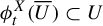 $\phi ^X_t(\overline {U})\subset U$
for any
 $t>0$
, and:
-
• there is a unique singularity
$\sigma _X\in U$
and it is hyperbolic; -
•
$C(\sigma _X,X)$
is the unique Lyapunov stable chain recurrence class contained in U; -
•
$C(\sigma _X,X)$
robustly contains a robust heterodimensional cycle; -
• the tangent bundle
$T_{C(\sigma _X,X)}M$
contains a two-dimensional subbundle
$E^X$
which is tangled and sectionally expanded; moreover,
$E^X$
is continuous in the following sense: if one fixes an arbitrary
$x\in C(\sigma ,X)$
, which is the limit of
$x_n\in C(\sigma _{X_n},X_n)$
with
$X_n\to X$
in the
$C^1$
topology, then the bundle
$E^{X_n}(x_n)$
converges to
$E^X(x)$
.






Remark 1.3. Since a robust heterodimensional cycle yields non-hyperbolic periodic orbits by arbitrarily small
 $C^1$
perturbations, the chain recurrence class
 $C(\sigma _X,X)$
for any
 $X\in \mathcal {V}$
is not singular hyperbolic or star.
Remark 1.4. Due to the upper semi-continuity of chain recurrence classes, the tangled subbundle
 $E^X$
varies only upper semi-continuously with respect to X.
Remark 1.5. In [Reference Bonatti, Li and Yang16], a non-empty
 $C^1$
open set of vector fields having an attractor containing singularities of different indices is constructed on a given 4-manifold. Their example exhibits also a robust heterodimensional cycle, but is accumulated by vector fields with homoclinic tangencies.
1.3 Idea of the construction
The example (in Theorem 1.2) is derived from a Lorenz attractor in the sense that the construction begins with the Lorenz attractor and uses a DA-type surgery. The Lorenz attractor, discovered by the meteorologist E. Lorenz in the early 1960s [Reference Lorenz36], is among the most important examples of singular flows. It is a chaotic attractor given by a simple group of three ordinary differential equations. We will consider the geometric model of the Lorenz attractor [Reference Afraimovich, Bykov and Shil’nikov2, Reference Guckenheimer and Williams31], which is equivalent to the original attractor for classical parameters [Reference Tucker56]. The DA surgery was introduced by Smale [Reference Smale55] as a way of constructing non-trivial basic sets, see also [Reference Williams59]. It has been used to give many inspiring and important examples, especially in the study of partially hyperbolic systems, see e.g. [Reference Bonatti and Viana18, Reference Mañé37].
In the following, we give some ideas of the construction.
We begin with a vector field
 $X^0$
on the 3-ball
 $B^3$
having a Lorenz attractor
 $\Lambda _0$
. Then, we consider a vector field
 $X(x,s)=(X^0(x),-\theta s)$
on the product
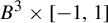 $B^3\times [-1,1]$
, where
 $(x,s)$
are coordinates on
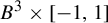 $B^3\times [-1,1]$
and
 $\theta>0$
is a constant. In particular, the dynamics is contracting along fibers. Note that
 $\Lambda =\Lambda _0\times \{0\}$
is an attractor and it contains a periodic orbit P.
Now, the idea is to modify the vector field X in a neighborhood of the periodic orbit P so that one obtains a robust heterodimensional cycle. For this purpose, we combine a DA-type surgery with the construction of a blender [Reference Bonatti, Díaz and Viana13]. Roughly speaking, a blender is a hyperbolic set which verifies some specific geometric properties so that its unstable manifold looks like a manifold of higher dimension. It naturally appears in the unfolding of a heterodimensional cycle of two periodic orbits and can be used to obtain robust heterodimensional cycles.
For this construction, we need to show that the obtained vector field is away from homoclinic tangencies. This requires a careful choice of the contraction rate
 $\theta $
along the fibers. Moreover, we need to show that the singularity and the heterodimensional cycle are contained in the same chain recurrence class. This constitutes the most difficult part of our proof.
1.4 Further discussions
For the example in Theorem 1.2, we would like to raise the following questions.
Question 1.6. Is the chain recurrence class
 $C(\sigma _X,X)$
(robustly) transitive? Or even isolated?
In addition to topological properties, one can also study ergodic properties of the example. In [Reference Shi, Yang and Yang53], it is proved that the entropy function for singular flows away from homoclinic tangencies is upper semi-continuous with respect to both invariant measures and the flows, provided that the limiting measure is not supported on singularities.
Question 1.7. Is the entropy function upper semi-continuous for the chain recurrence class
 $C(\sigma _X,X)$
in Theorem 1.2?
One may even consider existence of Sinai–Ruelle–Bowen (SRB) measures or physical measures. However, let us mention one difficulty in the study of this example. In contrast to the Lorenz attractor or a singular hyperbolic attractor, the usual analysis of the return map to a global cross-section may not be applicable in our example. This is because the chain recurrence class in our example admits a partially hyperbolic splitting
 $E^s\oplus F$
, where the three-dimensional center-unstable subbundle F contains a tangled two-dimensional subbundle and F is not sectionally expanded. Moreover, the subbundle F is not necessarily volume expanding.
Apart from the present example, it may also be interesting to consider a DA-type surgery on the two-sided Lorenz attractor constructed by Barros, Bonatti, and Pacifico [Reference Barros, Bonatti and Pacifico7].
The rest of this paper is organized as follows. We present some preliminaries of flows in §2 and give the construction of the example in §3. The proof of Theorem 1.2 is also given in §3, assuming some robust properties that will be proved in subsequent sections: in §4, we show that the example is away from homoclinic tangencies; then in §5, we show existence of a tangled subbundle; and finally in §6, we show that the singularity and the heterodimensional cycle are contained in the same chain recurrence class.
2 Preliminaries
In this section, we give some preliminaries on vector fields, including hyperbolicity, linear Poincaré flow, fundamental limit, and so on.
Let M be a compact Riemannian manifold without boundary. Let X be a
 $C^1$
vector field on M. Denote by
 $\operatorname {Sing}(X)$
the set of singularities, that is,
 $\operatorname {Sing}(X)=\{x\in M: X(x)=0\}$
. For any point
 $x\in M$
, we denote by
 $\langle X(x)\rangle $
the subspace of
 $T_xM$
that is generated by
 $X(x)$
. Note that
 $\langle X(x)\rangle $
is a one-dimensional subspace of
 $T_xM$
when
 $x\not \in \operatorname {Sing}(X)$
. To simplify notation, we also denote
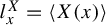 $l^X_x=\langle X(x)\rangle $
for
 $x\notin \operatorname {Sing}(X)$
.
2.1 Hyperbolicity
Recall that the flow and the tangent flow generated by X are denoted as
 $\phi _t$
and
 $\Phi _t$
, respectively. Let
 $\Lambda $
be a compact
 $\phi _t$
-invariant set and
 $E\subset T_{\Lambda }M$
a
 $\Phi _t$
-invariant subbundle. The dynamics
 $\Phi _t|_E$
is contracting, or E is contracted, if there exists constants
 $C\geq 1$
,
 $\unicode{x3bb}>0$
, such that
 $$ \begin{align*}\|\Phi_t|_{E(x)}\|\leq C{e}^{-\unicode{x3bb} t}\quad \text{for any}\ x\in \Lambda, \ t\geq 0.\end{align*} $$
One says that
 $\Phi _t|_E$
is expanding if
 $\Phi _{-t}|_E$
is contracting. The set
 $\Lambda $
is called hyperbolic if its tangent bundle admits a continuous splitting
 $T_{\Lambda }M=E^s\oplus \langle X\rangle \oplus E^u$
, where
 $\langle X\rangle $
is the subbundle generated by the vector field X, and
 $E^s$
(respectively
 $E^u$
) is contracted (respectively expanded). When
 $\Lambda $
is hyperbolic, for every
 $x\in \Lambda $
, the sets
 $$ \begin{align*}W^{ss}(x)=\{y\in M: \mathrm{dist}(\phi_t(x), \phi_t(y))\to 0\ \text{as}\ t\to +\infty\}\end{align*} $$
and
 $$ \begin{align*}W^{uu}(x)=\{y\in M: \mathrm{dist}(\phi_t(x), \phi_t(y))\to 0\ \text{as}\ t\to -\infty\}\end{align*} $$
are invariant
 $C^1$
submanifolds tangent to
 $E^s(x)$
and
 $E^u(y)$
, respectively, at x, see [Reference Hirsch, Pugh and Shub32]. We denote
 $W^s(\operatorname {Orb}(x))=\bigcup _{z\in \operatorname {Orb}(x)}W^{ss}(z)$
and
 $W^u(\operatorname {Orb}(x))=\bigcup _{z\in \operatorname {Orb}(x)}W^{uu}(z)$
, which are the stable and unstable manifolds of
 $\operatorname {Orb}(x)$
, respectively. For a chain transitive hyperbolic set, all stable manifolds
 $W^{ss}(x)$
have the same dimension
 $\operatorname {dim} E^s$
, which will be called the stable index of the hyperbolic set. Sometimes we simply say index with the same meaning of the stable index.
Flows with singularities, or singular flows, can exhibit complex dynamics with regular orbits accumulating on singularities, such as the famous Lorenz attractor [Reference Guckenheimer and Williams31, Reference Lorenz36]. In such cases, the set
 $\Lambda $
cannot be hyperbolic. Nevertheless, a weaker version of hyperbolicity can be defined. One says that
 $\Lambda $
is partially hyperbolic if there exists a
 $\Phi _t$
-invariant splitting of the tangent bundle
 $T_{\Lambda }M=E^s\oplus E^{cu}$
such that
 $E^s$
is contracted and it is dominated by
 $E^{cu}$
. If, moreover, the bundle
 $E^{cu}$
is sectionally expanded, then
 $\Lambda $
is said to be singular hyperbolic [Reference Morales, Pacifico and Pujals40]. Note that the partial hyperbolicity or singular hyperbolicity ensures also the existence of stable manifolds.
We will study mainly chain recurrence classes. A chain recurrence class
 $C(x,X)$
is non-trivial if it is not reduced to a critical element. In [Reference Pacifico, Yang and Yang43], it is shown that a non-trivial, Lyapunov stable, and singular hyperbolic chain recurrence class contains a periodic orbit, and
 $C^1$
generically, such a chain recurrence class is indeed an attractor. This result has been generalized to
 $C^1$
open and dense vector fields in [Reference Crovisier and Yang24].
2.2 Linear Poincaré flow and its extension
Given a
 $\phi _t$
-invariant set
 $\Lambda \subset M$
, define the normal bundle over
 $\Lambda $
as
 $$ \begin{align*} \mathcal{N}_{\Lambda}=\bigcup_{x\in\Lambda\setminus\operatorname{Sing}(X)}\mathcal{N}_x, \end{align*} $$
where
 $\mathcal {N}_x$
is the orthogonal complement of the one-dimensional subspace
 $l^X_x\subset T_xM$
generated by
 $X(x)$
. In particular, if
 $\Lambda =M$
, then
 $\mathcal {N}_M=\bigcup _{M\setminus \operatorname {Sing}(X)}\mathcal {N}_x$
. For any
 $x\in M\setminus \operatorname {Sing}(X)$
,
 $v\in \mathcal {N}_x$
, and
 $t\in {\mathbb R}$
, let
 $\psi _t(v)$
to be the orthogonal projection of
 $\Phi _t(v)$
to
 $\mathcal {N}_{\phi _t(x)}$
. In this way, one defines a flow
 $\psi _t=\psi ^X_t$
on the normal bundle
 $\mathcal {N}_M$
, which is called the linear Poincaré flow. Note that the normal bundle is not defined at singularities. Hence, the base of the normal bundle is non-compact for singular flows. We present below a compactification given by [Reference Li, Gan and Wen34].
Define the fiber bundle
 $G^1=\bigcup _{x\in M}Gr(1,T_xM)$
, where
 $Gr(1,T_xM)$
is the Grassmannian of lines in the tangent space
 $T_xM$
through the origin. Let
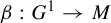 $\beta :G^1\to M$
be the corresponding bundle projection that sends a line
 $l\in Gr(1,T_xM)$
to x. The tangent flow
 $\Phi _t$
induces a flow
 $\hat {\Phi }_t$
on
 $G^1$
defined by
 $\hat {\Phi }_t(\langle v\rangle )=\langle \Phi _t(v)\rangle $
, where
 $v\in TM$
is a non-zero vector and
 $\langle v\rangle $
is the linear subspace spanned by v.
Let
 $\xi : TM\to M$
be the bundle projection of the tangent bundle. One then defines a vector bundle with base
 $G^1$
as
 $$ \begin{align*}\beta^*(TM)=\{(l,v)\in G^1\times TM: \beta(l)=\xi(v)\}.\end{align*} $$
The corresponding bundle projection
 $\iota $
sends every vector
 $(l,v)\in \beta ^*(TM)$
to l. The tangent flow induces also a flow
 $\tilde {\Phi }_t$
on
 $\beta ^*(TM)$
:
 $$ \begin{align*}\tilde{\Phi}_t(l,v)=(\hat{\Phi}_t(l),\Phi_t(v))\quad \text{for all } (l,v)\in\beta^*(TM).\end{align*} $$
The flow
 $\tilde {\Phi }_t$
will be called the extended tangent flow.
For any
 $l\in G^1$
such that
 $\beta (l)=x$
, there is a natural identification between
 $T_xM$
and
 $\{l\}\times T_xM$
. Thus, we define the extended normal bundle as
 $$ \begin{align*} \widetilde{\mathcal{N}}=\{(l,v)\in \beta^*(TM): v\perp l\}. \end{align*} $$
We also define the extended normal bundle over any non-empty subset
 $\Delta \subset G^1$
as
 $$ \begin{align*} \widetilde{\mathcal{N}}_{\Delta}=\{(l,v)\in\iota^{-1}(\Delta): v\perp l\}. \end{align*} $$
Finally, we define the extended linear Poincaré flow
 $\tilde {\psi }_t$
on
 $\widetilde {\mathcal {N}}$
as
 $$ \begin{align*} \tilde{\psi}_t(l,v)=\tilde{\Phi}_t(l,v)-\langle \Phi_t(u),\Phi_t(v)\rangle\cdot\tilde{\Phi}_t(l,u), \end{align*} $$
where
 $u\in l$
is a unit vector and
 $\langle \cdot ,\cdot \rangle $
stands for the inner product on the tangent bundle.
Remark 2.1. For any
 $x\notin \operatorname {Sing}(X)$
, let
 $l=l^X_x$
, then
 $\widetilde {\mathcal {N}}_l$
can be naturally identified with
 $\mathcal {N}_x$
and
 $\tilde {\psi }_t|_{\widetilde {\mathcal {N}}_l}$
can be naturally identified with
 $\psi _t|_{\mathcal {N}_x}$
.
We will also consider invariant measures on
 $G^1$
. Let
 $\mu $
be any Borel measure on
 $G^1$
. The bundle projection
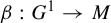 $\beta :G^1\to M$
induces a measure
 $\beta _*\mu $
on M such that
 $(\beta _*\mu )(A)=\mu (\beta ^{-1}(A))$
for any Borel set
 $A\subset M$
. When
 $\mu $
is
 $\hat {\Phi }_t$
-invariant, the induced measure
 $\beta _*\mu $
is
 $\phi _t$
-invariant.
2.3 Fundamental limit and dominated splitting
Given a chain recurrent set
 $\Gamma $
of the vector field X, let
 $X_n$
be a sequence of
 $C^1$
vector fields such that
 $X_n\to X$
in the
 $C^1$
topology. Suppose there exists a periodic orbit
 $\gamma _n$
of
 $X_n$
such that
 $\gamma _n$
converges to a compact subset of
 $\Gamma $
in the Hausdorff topology, then the sequence of pairs
 $(\gamma _n, X_n)$
is called a fundamental sequence of
 $\Gamma $
and will be denoted as
 $(\gamma _n,X_n)\hookrightarrow (\Gamma ,X)$
. The sequence
 $(\gamma _n,X_n)$
is called an i-fundamental sequence if
 $\operatorname {Ind}(\gamma _n)=i$
for all n large enough. When there is no possible ambiguity, we will simply say that
 $\gamma _n$
is a fundamental sequence of
 $\Gamma $
. We denote by
 $\mathcal {F}(\Gamma )$
the limit of directions of all fundamental sequences of
 $\Gamma $
, i.e.
 $$ \begin{align*}\mathcal{F}(\Gamma)=\{l\in G^1: \text{ there exists } (\gamma_n,X_n)\hookrightarrow (\Gamma,X),\ p_n\in \gamma_n \ \text{such that}\ l^{X_n}_{p_n} \to l\}.\end{align*} $$
As an immediate consequence of the definition, the map
 $\mathcal {F}(\cdot )$
is upper semi-continuous in the following sense.
Lemma 2.2. Suppose
 $\Gamma $
is a chain transitive set of X. Then, for any neighborhood
 $\mathcal {B}$
of
 $\mathcal {F}(\Gamma )$
in
 $G^1$
, there exist a neighborhood U of
 $\Gamma $
and
 $C^1$
neighborhood
 $\mathcal {U}$
of X such that for any
 $Y\in \mathcal {U}$
and any chain transitive set
 $\Gamma _Y$
of Y contained in U, it holds
 $\mathcal {F}(\Gamma _Y)\subset \mathcal {B}$
.
Proof. Arguing by contradiction, assume there exists a neighborhood
 $\mathcal {B}_0$
of
 $\mathcal {F}(\Gamma )$
and a sequence of vector fields
 $X_n$
converging to X in the
 $C^1$
topology, together with a sequence of chain transitive sets
 $\Gamma _n=\Gamma _{X_n}$
converging to a compact subset of
 $\Gamma $
in the Hausdorff topology, such that
 $\mathcal {F}(\Gamma _n)\not \subset \mathcal {B}_0$
for all n. By choosing a subsequence, assume that
 $\mathcal {F}(\Gamma _n)$
converges in the Hausdorff topology to
 $\mathcal {B}_1$
. Then,
 $\mathcal {B}_1\setminus \mathcal {B}_0\neq \emptyset $
. By definition of the map
 $\mathcal {F}(\cdot )$
, there exists a fundamental sequence
 $(\gamma _n,X_n)\hookrightarrow (\Gamma ,X)$
such that
 $\mathcal {F}(\gamma _n)$
accumulates on a point
 $l\in \mathcal {B}_1\setminus \mathcal {B}_0$
. This is a contradiction since
 $l\in \mathcal {F}(\Gamma )\subset \mathcal {B}_0$
.
We also denote by
 $B(\Gamma )$
the limit set of directions of regular points contained in
 $\Gamma $
, i.e.
 $$ \begin{align*}B(\Gamma)=\{l\in G^1: \text{ there exists } x_n\in \Gamma\setminus\operatorname{Sing}(X) \ \text{such that}\ l^X_{x_n} \to l\}.\end{align*} $$
Note that for any
 $l\in \mathcal {F}(\Gamma )$
, if
 $x=\beta (l)$
is a regular point, then
 $l=l^X_x$
. This also holds for
 $B(\Gamma )$
. Thus,
 $\mathcal {F}(\Gamma )\setminus B(\Gamma )$
is contained in the tangent spaces of singularities.
A hyperbolic singularity
 $\rho $
is called Lorenz-like if there is a partially hyperbolic splitting of the tangent bundle
 $T_{\rho }M=E^{ss}_{\rho }\oplus E^{cu}_{\rho }$
such that
 $E^{cu}_{\rho }$
is sectionally expanded and it decomposes further into a dominated splitting
 $E^c_{\rho }\oplus E^u_{\rho }$
with
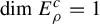 $\operatorname {dim} E^c_{\rho }=1$
and
 $\Phi _t|_{E^c_{\rho }}$
is contracting. For a Lorenz-like singularity
 $\rho $
, denote by
 $W^{ss}(\rho )$
its strong stable manifold tangent to
 $E^{ss}_{\rho }$
at the singularity.
Lemma 2.3. Let
 $C(\rho ,X)$
be a chain recurrence class of X containing a Lorenz-like singularity
 $\rho $
such that
 $C(\rho ,X)\cap (W^{ss}(\rho )\setminus \{\rho \})=\emptyset $
. Then, there exists a
 $C^1$
neighborhood
 $\mathcal {U}$
of X such that for any
 $Y\in \mathcal {U}$
, it holds
 $C(\rho _Y,Y)\cap (W^{ss}(\rho _Y,Y)\setminus \{\rho _Y\})=\emptyset $
and
 $\mathcal {F}(C(\rho _Y,Y))\cap T_{\rho _Y}M\subset E^{cu}_{\rho _Y}$
. (Here, to simplify notation, we have identified
 $T_{\rho _Y}M$
with
 $Gr(1,T_{\rho _Y}M)$
and
 $E^{cu}_{\rho _Y}$
with
 $Gr(1,E^{cu}_{\rho _Y})$
. We hope that such abuses of notation shall not cause much confusion.)
Proof. Note that the properties defining a Lorenz-like singularity is
 $C^1$
robust. Since the singularity
 $\rho $
is Lorenz-like, there is a
 $C^1$
neighborhood
 $\mathcal {U}$
of X such that for any
 $Y\in \mathcal {U}$
, the continuation
 $\rho _Y$
is also Lorenz-like. Moreover, by the upper semi-continuity of chain recurrence class and the continuity of local strong stable manifolds, one deduces that
 $C(\rho _Y,Y)\cap (W^{ss}(\rho _Y,Y)\setminus \{\rho _Y\})=\emptyset $
for any
 $Y\in \mathcal {U}$
(shrinking
 $\mathcal {U}$
if necessary). Then, a similar argument as in the proof of [Reference Li, Gan and Wen34, Lemma 4.4] gives
 $\mathcal {F}(C(\rho _Y,Y))\cap T_{\rho _Y} M\subset E^{cu}_{\rho _Y}$
.
Remark 2.4. Regarding the proof, we would like to provide further clarification. In examining the proof of [Reference Li, Gan and Wen34, Lemma 4.4], one will notice that the argument involves a local analysis of the dynamics within a small neighborhood of the singularity. The key insight is that regular points of the strong homogeneous set (which corresponds to the chain recurrence class in our work) cannot accumulate at the singularity along its strong stable direction.
A fundamental sequence
 $(\gamma _n,X_n)$
of
 $\Gamma $
is said to admit an index i dominated splitting if there exist a
 $\psi ^{X_n}_t$
-invariant splitting
 $\mathcal {N}_{\gamma _n}=\mathcal {N}_n^{cs}\oplus \mathcal {N}_n^{cu}$
(
 $n\in \mathbb {N}$
) of the normal bundle and constants
 $T>0$
,
 $n_0>0$
such that for any
 $t>T$
and
 $n>n_0$
, it holds
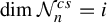 $\operatorname {dim} \mathcal {N}_n^{cs}=i$
and for any
 $x\in \gamma _n$
,
 $$ \begin{align*}\|\psi^{X_n}_t|_{\mathcal{N}_n^{cs}(x)}\|\cdot\|\psi^{X_n}_{-t}|_{\mathcal{N}_n^{cu}(\phi^{X_n}_t(x))}\|<1/2.\end{align*} $$
Identifying the extended normal bundle
 $\widetilde {\mathcal {N}}_{B(\gamma _n)}$
with
 $\mathcal {N}_{\gamma _n}$
(see Remark 2.1), we see that
 $\widetilde {\mathcal {N}}_{B(\gamma _n)}$
also admits a dominated splitting with respect to
 $\tilde {\psi }_t^{X_n}$
and of the same index. Note that
 $B(\gamma _n)$
converges to a compact subset of
 $\mathcal {F}(\Gamma )$
in the Hausdorff topology of the Grassmannian
 $G^1$
. Thus, the following lemma is a consequence of the property that a dominated splitting can be extended to the closure and to a neighborhood (see e.g. [Reference Bonatti, Díaz and Viana13, Appendix B]) and its proof will be omitted.
Lemma 2.5. The set
 $\mathcal {F}(\Gamma )$
admits a dominated splitting of index i with respect to
 $\tilde {\psi }^X_t$
if and only if every fundamental sequence of
 $\Gamma $
admits an index i dominated splitting with the same domination constant T.
3 The example: construction and robust properties
In this section, we construct the example and claim some key properties of the example. With these properties, a proof of Theorem 1.2 is given at the end of this section.
3.1 The Lorenz attractor
Let us begin with the geometric model of the Lorenz attractor, see e.g. [Reference Bonatti, Díaz and Viana13, Reference Guckenheimer and Holmes30, Reference Guckenheimer and Williams31]. Let
 $(x_1,x_2,x_3)$
be a Cartesian coordinate system in
 ${\mathbb R}^3$
. Let
 $B^3$
be a ball in
 $\mathbb {R}^3$
centered at the origin
 $O=(0,0,0)$
. We shall consider a
 $C^1$
vector field
 $X^0$
on
 ${\mathbb R}^3$
such that it is transverse to the boundary of
 $B^3$
and that the ball
 $B^3$
is an attracting region, that is,
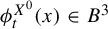 $\phi _t^{X^0}(x)\in B^3$
for any
 $x\in B^3$
and
 $t>0$
. Moreover, the following properties are assumed (see [Reference Araújo and Pacifico4, §3]).
(P1) (Lorenz-like singularity). The origin O is a hyperbolic singularity of stable index 2 such that its local stable manifold
 $W^s_{\mathrm {loc}}(O)$
coincides with the
 $x_1x_3$
-plane, and its local unstable manifold
 $W^u_{\mathrm {loc}}(O)$
coincides with the
 $x_2$
-axis. Moreover, the two-dimensional stable subspace
 $E^s_O$
decomposes into a dominated splitting
 $E^s_O=E^{ss}_O\oplus E^{c}_O$
. Assume that the local strong stable manifold (tangent to
 $E^{ss}_O$
) coincides with the
 $x_1$
-axis. The three Lyapunov exponents at the singularity are
 $$ \begin{align*} \unicode{x3bb}^s=\log\|D\Phi^{X^0}_1|_{E^{ss}_O}\|,\quad \unicode{x3bb}^c=\log\|D\Phi^{X^0}_1|_{E^{c}_O}\|\quad \text{and}\quad \unicode{x3bb}^u=\log\|D\Phi^{X^0}_1|_{E^{u}_O}\|. \end{align*} $$
Here,
 $E^u_O$
is the unstable subspace of O. One has
 $\unicode{x3bb} ^s<\unicode{x3bb} ^c<0<\unicode{x3bb} ^u$
. We assume that
 $\unicode{x3bb} ^c+\unicode{x3bb} ^u>0$
, which implies sectional expanding property of the subspace
 $E^{cu}_O=E^{c}_O\oplus E^u_O$
.
(P2) (Cross-section and the first return map). The square
 $\Sigma _0=\{(x_1,x_2,1): -1\leq x_1, x_2\leq 1\}$
is a cross-section of the flow
 $\phi ^{X^0}_t$
, meaning that the vector field at every point of
 $\Sigma _0$
is transverse to
 $\Sigma _0$
. For simplicity, we assume that the vector field is orthogonal to
 $\Sigma _0$
and
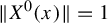 $\|X^0(x)\|=1$
for any
 $x\in \Sigma _0$
. The cross-section
 $\Sigma _0$
intersects
 $W^s_{\mathrm {loc}}(O)$
at a line segment
 $L_0=\{(x_1,0,1): -1\leq x_1\leq 1\}$
, which cuts
 $\Sigma _0$
into a left part
 $\Sigma _0^-$
and a right part
 $\Sigma _0^+$
,
 $\Sigma _0\setminus L_0=\Sigma _0^-\cup \Sigma _0^+$
. There is a first return map
 $R_0: \Sigma _0\setminus L_0\to \Sigma _0$
such that the images
 $R_0(\Sigma _0^-)$
and
 $R_0(\Sigma _0^+)$
are each a square pinched at one end and contained in the interior of
 $\Sigma _0$
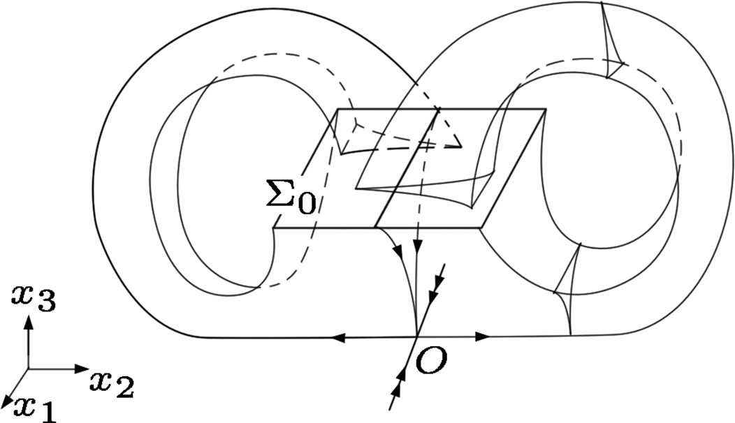
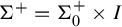
, as shown in Figure 1. Let us assume that for any
 $x\in \Sigma _0\setminus L_0$
, the time
 $t_x>0$
satisfying
 $\phi ^X_{t_x}(x)=R_0(x)$
for its first return is at least 2, that is,
 $t_x>2$
.
The Lorenz attractor.

(P3) (Cone field on the cross-section). For each
 $\alpha>0$
, there is a cone
 $C_{\alpha }(x)$
at the point
 $x=(0,0,1)$
:
 $$ \begin{align*}C_{\alpha}(x)=\{(x_1,x_2)\in T_{x}\Sigma_0 : \|x_1\|\leq \alpha\|x_2\|\}.\end{align*} $$
Here, we have identified
 $T_x\Sigma _0$
with
 $\Sigma _0$
and use the same coordinates
 $x_1,x_2$
. By translating
 $C_{\alpha }(x)$
to every other point on
 $\Sigma _0$
, one defines a cone field
 $C_{\alpha }$
on
 $\Sigma _0$
. We assume that
 $R_0$
preserves the cone
 $C_{\alpha }$
with
 $\alpha =1$
. More precisely, for any
 $x\in \Sigma _0\setminus L_0$
and any vector
 $u\in C_1(x)$
, we assume
 $DR_0(u)\in C_{1/2}(R_0(x))$
.
(P4) (The attractor). Let
 $\Lambda _0=\mathrm { Cl}(\phi ^{X^0}_{t\in \mathbb {R}}(\Lambda _{\Sigma _0}))$
, where
 $\Lambda _{\Sigma _0}=\bigcap _{n\geq 0}\overline {R_0}^n(\Sigma _0)$
and
 $\overline {R_0}^n(\Sigma _0)$
is the closure of the nth return of
 $\Sigma _0$
, ignoring
 $L_0$
for each return. Then,
 $\Lambda _0$
contains O and is the unique attractor in
 $B^3$
, with an attracting neighborhood
 $U_{\Lambda _0}\subset B^3$
that contains
 $\Sigma _0$
.
(P5) (Singular hyperbolicity). The attractor
 $\Lambda _0$
admits a singular hyperbolic splitting
 $T_{\Lambda _0}{\mathbb R}^3=E^{ss}\oplus E^{cu}$
, where
 $E^{ss}$
is uniform contracted and
 $E^{cu}$
is sectionally expanded. Precisely, we assume that for any two-dimensional subspace
 $S\subset E^{cu}_x$
,
 $x\in \Lambda _0$
, it holds
 $$ \begin{align} \Big|\!\det(\Phi^{X^0}_t|_S)\Big|>e^{\gamma t}\quad \text{for all } t\geq 1, \end{align} $$
where
 $\gamma>0$
is a constant. The constant
 $\gamma $
will be assumed to be large so that the inequality (3.1) implies expanding property for the first return map
 $R_0$
: there exists
 $\rho>1$
such that for any
 $x\in \Lambda _0\cap (\Sigma _0\setminus L_0)$
,
 $v\in E^{cu}_x\cap (T_x\Sigma _0\setminus \{0\})$
, it holds
 $$ \begin{align*}\|DR_0(v)\|>\rho\|v\|.\end{align*} $$
As the flow direction
 $X^0$
is invariant and cannot be uniformly contracted, it is contained in the subbundle
 $E^{cu}$
, that is,
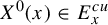 ${X^0}(x)\in E^{cu}_x$
for every
 $x\in \Lambda _0\setminus \operatorname {Sing}(X)$
(see [Reference Bonatti, Gan and Yang15, Lemma 3.4]). At the singularity O, we have
 $E^{cu}_O=E^{c}_O\oplus E^u_O$
. Define
 $$ \begin{align*}\unicode{x3bb}^s_0=\log\|D\Phi^{X^0}_1|_{E^{ss}_{\Lambda_0}}\|.\end{align*} $$
Note that
 $\unicode{x3bb} ^s\leq \unicode{x3bb} ^s_0$
. We assume
 $\unicode{x3bb} ^s_0<\unicode{x3bb} ^c$
.
(P6) (Stable foliation). The stable foliation
 $\mathcal {W}^s(\Lambda _0)=\{W^s(\operatorname {Orb}(x)): x\in \Lambda _0\}$
is
 $C^1$
(see [Reference Araújo and Melbourne3]), which induces a
 $C^1$
foliation
 $\mathcal {F}^s$
on
 $\Sigma _0$
such that for any
 $x\in \Sigma _0$
,
 $\mathcal {F}^s(x)$
is transverse to
 $C_1(x)$
. Since
 $L_0$
is the intersection of
 $W^s_{\mathrm {loc}}(O)$
with
 $\Sigma _0$
, it is a leaf of
 $\mathcal {F}^s$
.
(P7) (Transitivity). The attractor
 $\Lambda _0$
is a homoclinic class (see [Reference Bautista8, Reference Guckenheimer and Williams31]), so that
 $\Lambda _0$
is transitive and there is a periodic orbit
 $Q_0\subset \Lambda _0$
whose stable manifold is dense in
 $U_{\Lambda _0}$
.
3.2 The skew product construction
Let
 $\Omega =B^3\times I$
, where
 $I=[-1,1]$
. Let x, s be the coordinates on
 $B^3$
and I, respectively. Define on
 $\Omega $
the vector field
 $\hat {X}(x,s)=(X^0(x),-\theta s)$
, where
 $\theta>0$
is a constant. As the fiber direction (along I) is uniformly contracting, there exists a unique attractor
 $\Lambda =\Lambda _0\times \{0\}$
, which is a trivial construction of the Lorenz attractor in dimension 4. All properties of the three-dimensional attractor
 $\Lambda _0$
can be easily generalized to
 $\Lambda $
. In the following, we will modify the vector field
 $\hat {X}$
along fibers to obtain a vector field X such that
 $\Lambda $
remains an attractor but not singular hyperbolic. This is why we refer to the example as being derived from the Lorenz attractor. It may be of interest to compare our example with the construction of Lorenz attractors with arbitrary expanding dimensions presented by Bonatti et al [Reference Bonatti, Pumariño and Viana17].
The modification will be done in a small neighborhood of a periodic orbit in
 $\Lambda $
. Let
 $P_0\subset \Lambda _0$
be a periodic orbit of
 $X^0$
other than
 $Q_0$
such that it is homoclinically related to
 $Q_0$
. Let
 $P=P_0\times \{0\}$
and
 $Q=Q_0\times \{0\}$
. Consider a small neighborhood
 $V_P$
of P contained in
 $U_{\Lambda _0}\times (-1,1)$
such that
 $\overline {V_P}\cap (Q\cup \{\sigma \})=\emptyset $
, where
 $\sigma =(O,0)$
. Let
 $\eta $
be a
 $C^{\infty }$
function on
 $M_0$
that satisfies the following conditions:
-
•
$0\leq \eta (x,s)\leq 1$
for all
$(x,s)\in \Omega $
; -
•
$\eta $
is supported on
$V_P$
, that is,
$\eta (x,s)=0$
for any
$(x,s)\not \in V_P$
; -
•
$\eta (x,s)=1$
if and only if
$(x,s)\in P$
.



The vector field X on
 $\Omega $
is defined as the following:
 $$ \begin{align} X(x,s)=(X^0(x), -\theta s(1-\eta(x,s))). \end{align} $$
Observe that the dynamics of the vector field is contracting along the fibers, except only for P where it is neutral. Also,
 $U_{\Lambda }=U_{\Lambda _0}\times (-1,1)$
is an attracting region of X and the maximal invariant set
 $\Lambda =\Lambda _0\times \{0\}$
in
 $U_{\Lambda }$
is an attractor. The attractor contains a unique singularity
 $\sigma =(O,0)$
. The tangent space at
 $\sigma $
admits a
 $\Phi ^X_t$
-invariant splitting
 $T_{\sigma }\Omega =T_{\sigma }B^3\oplus {\mathbb R}^I$
, in which we identify
 $B^3$
with
 $B^3\times \{0\}$
and
 ${\mathbb R}^I$
is the subspace corresponding to the fiber. Thus, the Lyapunov exponents of
 $\sigma $
are
 $\unicode{x3bb} ^s, \unicode{x3bb} ^c, \unicode{x3bb} ^u$
, and
 $-\theta $
. Note that
 $-\theta $
is the Lyapunov exponent of the singularity along the fiber direction. We assume further that

This implies in particular that there is a dominated splitting of the stable subspace
 $E^s_{\sigma }=E^{ss}\oplus {\mathbb R}^I\oplus E^{cs}$
. The following properties can be easily verified.
-
(C1) The cube
$\Sigma =\Sigma _0\times I$
is a cross-section of the flow
$\phi ^X_t$
. The local stable manifold of
$\sigma $
cuts
$\Sigma $
along a two-dimensional disk
$L=L_0\times I$
. So
$\Sigma \setminus L$
consists of a left part
$\Sigma ^-=\Sigma _0^-\times I$
and a right part
$\Sigma ^+=\Sigma _0^+\times I$
. Let
$R:\Sigma \setminus L\to \Sigma $
be the first return map. Then,
$R(\Sigma ^-)$
is a cube pinched at one end and contained in the interior of
$\Sigma $
, and similarly for
$R(\Sigma ^+)$
. For any
$p\in \Sigma \setminus L$
, let
$t_p>0$
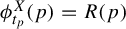
be the smallest time that
$\phi ^X_{t_p}(p)=R(p)$
. By assumption on
$R_0$
, we have
$t_p>2$
for any
$p\in \Sigma \setminus L$
. -
(C2) Q is a hyperbolic periodic orbit contained in
$\Lambda $
with stable index 2. The stable manifold
$W^s(Q,X)$
is dense in
$U_{\Lambda }$
. This follows from the fact that the stable manifold of the periodic orbit
$Q_0$
is dense in
$U_{\Lambda _0}$
and that the tangent flow along the fibers is topologically contracting. Moreover,
$W^s(Q,X)$
intersects
$\Sigma $
along a dense family of two-dimensional
$C^1$
disks, which are leaves of the foliation
$\mathcal {F}^s\times I$
. Here,
$\mathcal {F}^s$
is the foliation on
$\Sigma _0$
as in Property (P6). -
(C3)
$P\subset \Lambda $
is a non-hyperbolic periodic orbit of X: it has a zero exponent along the fiber direction. Nonetheless, P has a three-dimensional topologically stable manifold and its strong stable manifold
$W^{ss}(P,X)$
(two-dimensional) has non-empty intersection with the unstable manifold of Q. Also, its unstable manifold has a transverse intersection with the stable manifold of Q.











3.3 Robust properties of the example
As a first result, we show that
 $\Lambda $
admits a partially hyperbolic splitting.
Lemma 3.1. There exists a partially hyperbolic splitting
 $T_{\Lambda }\Omega =E^{ss}\oplus F$
for the tangent flow with
 $\operatorname {dim} E^{ss}=1$
.
Proof. Since
 $T_{\Lambda }\Omega =T_{\Lambda _0}B^3\oplus {\mathbb R}^I$
and
 $T_{\Lambda _0}B^3$
admits a partially hyperbolic splitting
 $E^{ss}\oplus E^{cu}$
, one obtains an invariant splitting
 $T_{\Lambda }\Omega =E^{ss}\oplus F$
, where
 $F=E^{cu}\oplus {\mathbb R}^I$
. Since
 $E^{ss}$
is already dominated by
 $E^{cu}$
, (3.3) implies that
 $E^{ss}$
is dominated by F. Moreover,
 $\Phi ^X_t|_{E^{ss}}$
is contracting as it can be identified with
 $\Phi ^{X_0}_t|_{E^{ss}}$
. Hence,
 $T_{\Lambda }\Omega =E^{ss}\oplus F$
is a partially hyperbolic splitting.
Note that the splitting
 $F=E^{cu}\oplus {\mathbb R}^I$
is invariant but not dominated (in F). This is because the bundle
 ${\mathbb R}^I$
is neutral on the periodic orbit
 $P=P_0\times \{0\}$
and cannot be dominated by the bundle
 $E^{cu}$
which contains the flow direction, and vice versa. Also, F is not sectionally expanded; hence,
 $\Lambda $
is not singular hyperbolic. Nonetheless, the invariance of the splitting
 $T_{\Lambda }\Omega =E^{ss}\oplus E^{cu}\oplus {\mathbb R}^I$
suggests also an invariant splitting of the extended normal bundle with one-dimensional subbundles.
Proposition 3.2. The extended normal bundle
 $\widetilde {\mathcal {N}}_{\mathcal {F}(\Lambda )}$
admits a dominated splitting
 $\mathcal {N}^{ss}\oplus \mathcal {N}^I\oplus \mathcal {N}_2$
with one-dimensional subbundles. Consequently,
 $X|_{\Lambda }$
is
 $C^1$
locally away from homoclinic tangencies.
Here, a chain recurrence class is called locally away from homoclinic tangencies if there exists a neighborhood U of the class and a
 $C^1$
neighborhood
 $\mathcal {U}$
of X such that any
 $Y\in \mathcal {U}$
admits no homoclinic tangency in U.
Also, the sectionally expanding subbundle
 $E^{cu}$
in the splitting
 $T_{\Lambda }\Omega =E^{ss}\oplus E^{cu}\oplus {\mathbb R}^I$
will be shown to exist robustly in the following sense.
Proposition 3.3. There exist a neighborhood
 $U\subset U_{\Lambda }$
of
 $\Lambda $
and a neighborhood
 $\mathcal {U}$
of X such that for any
 $Y\in \mathcal {U}$
and any chain recurrence class
 $C_Y\subset U$
, there is a continuous two-dimensional subbundle
 $E^Y$
of
 $T_{C_Y}\Omega $
containing the flow direction such that it is invariant for
 $\Phi ^Y_t$
and sectionally expanded. Moreover, if
 $C_Y=C(\sigma _Y,Y)$
is the chain recurrence class containing
 $\sigma _Y$
, then
 $E^Y$
varies continuously with respect to
 $Y\in \mathcal {U}$
in the following sense: given
 $x\in C_Y$
, which is the limit of
 $x_n\in C(\sigma _{Y_n},Y_n)$
with
 $Y_n\to Y$
in the
 $C^1$
topology, then
 $E^{Y_n}(x_n)\to E^Y(x)$
.
The proofs of Propositions 3.2 and 3.3 will be given in §§4 and 5, respectively.
By construction, the chain recurrence class
 $\Lambda $
is an attractor containing the unique singularity
 $\sigma =(O,0)$
. We will show that for any
 $C^1$
vector field Y close enough to X, the chain recurrence class
 $C(\sigma _Y,Y)$
is non-trivial and Lyapunov stable. Moreover, it is the only Lyapunov stable chain recurrence class in
 $U_{\Lambda }$
, where
 $\sigma _Y$
is the continuation of the singularity. Precisely, we have the following proposition.
Proposition 3.4. There exists a
 $C^1$
neighborhood
 $\mathcal {U}$
of X such that for any
 $Y\in \mathcal {U}$
, the chain recurrence class
 $C(\sigma _{Y},Y)$
is the unique Lyapunov stable chain recurrence contained in
 $U_{\Lambda }$
. Moreover,
 $C(\sigma _{Y},Y)$
contains the periodic orbit
 $Q_Y$
, which is the continuation of Q.
3.4 Robust heterodimensional cycles
Before we continue with the construction of the example, let us recall that a vector field is said to have a heterodimensional cycle associated with two transitive hyperbolic sets
 $\Gamma $
and
 $\Gamma '$
if:
-
• the indices of
$\Gamma $
and
$\Gamma '$
are different; and -
• the stable manifold of
$\Gamma $
intersects the unstable manifold of
$\Gamma '$
and vice versa.


The heterodimensional cycle is robust if there is a
 $C^1$
-neighborhood
 $\mathcal {U}$
of the vector field such that every
 $Y\in \mathcal {U}$
has a heterodimensional cycle associated with the hyperbolic sets
 $\Gamma _{Y}$
and
 $\Gamma ^{\prime }_Y$
, where
 $\Gamma _{Y}$
and
 $\Gamma ^{\prime }_Y$
are the continuations of
 $\Gamma $
and
 $\Gamma '$
, respectively.
We will prove the following result.
Lemma 3.5. In every
 $C^1$
neighborhood of X, there is an open subset
 $\mathcal {V}$
of vector fields such that for each
 $Y\in \mathcal {V}$
, the chain recurrence class
 $C(\sigma _{Y},Y)$
robustly contains a robust heterodimensional cycle.
Remark 3.6. By the lemma, the vector field X can be
 $C^1$
approximated by vector fields with robust heterodimensional cycles. Also, it follows from the construction that X can be
 $C^1$
approximated by vector fields with singular hyperbolic attractors. Therefore, X is on the boundary between singular hyperbolicity and robust heterodimensional cycles.
The proof of Lemma 3.5 is essentially contained in [Reference Bonatti and Díaz11, §4]. We say that a periodic orbit is a pre-saddle if its normal bundle has an (orientable) one-dimensional center along which the Lyapunov exponent is zero, and all other Lyapunov exponents are non-zero. For the vector field X, the periodic orbit P is a pre-saddle with a one-dimensional center in the fiber direction, along which the Lyapunov exponent is zero. The pre-saddle P has a strong stable manifold
 $W^{ss}(P,X)$
contained in
 $B^3\times \{0\}$
(as in the three-dimensional Lorenz attractor). Also, its unstable manifold
 $W^u(P,X)$
is contained in
 $B^3\times \{0\}$
. By the skew product construction of our example,
 $P=P_0\times \{0\}$
and
 $P_0$
exhibits homoclinic intersections, which are exactly the intersections of
 $W^{ss}(P,X)$
and
 $W^u(P,X)$
. Such intersections will be called strong homoclinic intersections associated to P. Moreover, each strong homoclinic intersection r is quasi-transverse:
 $\operatorname {dim} (T_rW^{ss}(P,X)\oplus T_rW^u(P,X))=3<\operatorname {dim} \Omega =4$
. The next result shows how to obtain robust heterodimensional cycles. See also [Reference Li and Turaev33] for more recent progress on this topic.
Lemma 3.7. [Reference Bonatti and Díaz11, Theorem 2.4]
Let X be a
 $C^1$
vector field with a quasi-transverse strong homoclinic intersection associated to a pre-saddle. Then, in every
 $C^1$
neighborhood of X, there is an open set of vector fields exhibiting robust heterodimensional cycles.
Remark 3.8. The lemma restates the mechanism proposed by Bonatti and Díaz for obtaining robust heterodimensional cycles in diffeomorphisms. We want to emphasize that this mechanism applies to the dynamics within a small neighborhood of a homoclinic orbit associated with a periodic orbit (a pre-saddle). Importantly, this can be achieved away from singularities. A similar approach has also been used by Li and Turaev [Reference Li and Turaev33]. This provides sufficient evidence that the mechanism of Bonatti and Díaz is applicable to vector fields as well.
It follows from the previous discussions and Lemma 3.7 that there exists vector field Y arbitrarily close to X which exhibits a robust heterodimensional cycle. Thus, to prove Lemma 3.5, it remains to show that the robust heterodimensional cycle is contained in
 $C(\sigma _{Y},Y)$
. For this, we need to slightly change the proof of Lemma 3.7 [Reference Bonatti and Díaz11, §4], in which a key ingredient is the creation of robust heterodimensional cycles through blenders. Roughly speaking, a blender is a hyperbolic set whose stable (or unstable) set behaves as if it is one dimension higher than it actually is. One can refer to e.g. [Reference Bonatti, Díaz and Viana13, Ch. 6] for more discussions on blenders.
Proof of Lemma 3.5
We have seen that the periodic orbit P is a pre-saddle associated to which there is a quasi-transverse strong homoclinic intersection. In fact, we can take two quasi-transverse strong homoclinic intersections z and w associated to P such that their orbits are disjoint. This is because the strong homoclinic intersections correspond to the homoclinic intersections of
 $P_0$
, which are known to have infinitely many points with mutually disjoint orbits. Following the proof of Lemma 3.7 [Reference Bonatti and Díaz11, §4], one can make arbitrarily small
 $C^1$
perturbations in a neighborhood of
 $\mathrm {Cl}(\operatorname {Orb}(z,X)\cup \operatorname {Orb}(w,X))$
(containing P) to obtain a vector field Y having a blender
 $\Lambda '$
, together with a hyperbolic periodic orbit
 $P_{\delta }$
close to
 $P_Y$
such that:
-
• the blender
$\Lambda '$
is a hyperbolic set of stable index
$1$
containing the periodic orbit
$P_Y$
; -
• the periodic orbit
$P_{\delta }$
has stable index
$2$
, and its stable manifold intersect transversely the unstable manifold of
$P_Y$
; -
• the unstable manifold of
$P_{\delta }$
meets robustly the stable set of the blender
$\Lambda '$
(by the property of the blender); -
• thus, the vector field Y has a robust heterodimensional cycle associated with the hyperbolic set
$\Lambda '\supset P_Y$
and the hyperbolic saddle
$P_{\delta }$
.


One can see that
 $C(\sigma _Y,Y)$
contains the robust heterodimensional cycle if it contains
 $P_{\delta }$
.
We can assume that Y is close enough to X so that by Proposition 3.4,
 $C(\sigma _Y,Y)$
is Lyapunov stable and contains the periodic orbit
 $Q_Y$
. Thus, to guarantee that
 $C(\sigma _Y,Y)$
contains
 $P_{\delta }$
and hence the robust heterodimensional cycle, we need only show that
 $W^u(Q_Y,Y)\pitchfork W^s(P_{\delta },Y)\neq \emptyset $
. A slightly different procedure should be followed when making the perturbations to obtain the robust heterodimensional cycle.
Recall that in [Reference Bonatti and Díaz11, §4],
 $P_{\delta }$
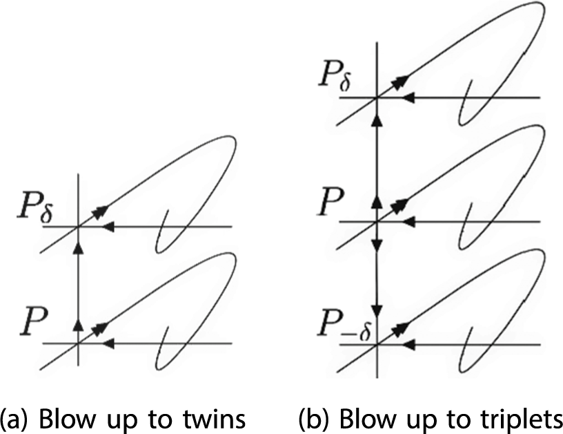
is obtained as a twin of P by blowing up the pre-saddle P along the neutral center, as shown in Figure 2(a). Instead of obtaining only a twin
 $P_{\delta }$
, we blow up the pre-saddle to obtain a set of triplet saddles, P,
 $P_{\delta }$
, and
 $P_{-\delta }$
, as shown in Figure 2(b). See also [Reference Mañé37] for a similar construction. The saddles
 $P_{\delta }$
and
 $P_{-\delta }$
are both of index 2, while P has index 1. Note that for the vector X, there is a quasi-transverse intersection between
 $W^u(Q,X)$
and
 $W^{ss}(P,X)$
. After the blow-up, one has either
 $W^u(Q_Y,Y)\pitchfork W^s(P_{\delta },Y)\neq \emptyset $
or
 $W^u(Q_Y,Y)\pitchfork W^s(P_{-\delta },Y)\neq \emptyset $
. By interchanging the notation, we can assume without loss of generality that
 $W^u(Q_Y,Y)\pitchfork W^s(P_{\delta },Y)\neq \emptyset $
. Then, the construction continues as in [Reference Bonatti and Díaz11, §4].
DA-type surgery at the pre-saddle P.

As argued before, the construction ensures that
 $C(\sigma _Y,Y)$
contains the robust heterodimensional cycle associated with a blender and the hyperbolic saddle
 $P_{\delta }$
. Note also that this property for Y is robust. The proof of Lemma 3.5 is now complete as Y can be chosen to be arbitrarily
 $C^1$
close to X.
3.5 Proof of Theorem 1.2
Let M be any four-dimensional closed Riemannian manifold. One considers a gradient-like vector field
 $Z_0$
on M, which has at least a sink. Consider a local chart around a sink and a ball
 $B^4$
in the chart, centered at the sink. By shrinking the local chart, we assume that the ball
 $B^4$
is an attracting region of the flow. In particular, the vector field
 $Z_0$
is transverse to
 $\partial B^4$
and inwardly pointing. By changing the metric, we assume that
 $\tfrac 12B^4$
contains
 $\Omega =B^3\times [-1,1]$
. Let X be a vector field on
 $\Omega $
as constructed in §§3.1 and 3.2. Let us denote by
 $\tfrac 12B^4$
the ball with the same center of
 $B^4$
and half the radius. One then modifies the vector field
 $Z_0$
in a neighborhood of
 $\tfrac 12B^4$
to obtain a
 $C^1$
vector field Z such that it coincides with X on
 $\Omega \subset \tfrac 12B^4$
. The modification shall be taken outside a neighborhood of
 $M\setminus B^4$
; thus, Z coincides with
 $Z_0$
in a neighborhood of
 $M\setminus B^4$
. Moreover, since the vector field on
 $\Omega $
is transverse to each smooth component of
 $\partial \Omega $
and inwardly pointing, one can require that the obtained vector field Z has no recurrence in
 $B^4\setminus \Omega $
. Then, the chain recurrence set of Z is composed of finitely many hyperbolic critical elements and the maximal invariant set in
 $\Omega $
.
The following properties can be verified.
-
(1) There is a non-trivial chain recurrence class
$C(\sigma ,Z)$
associated to a hyperbolic singularity
$\sigma \in \Omega $
. -
(2) There exist a neighborhood
$U\subset \Omega $
of
$C(\sigma ,Z)$
and a neighborhood
$\mathcal {U}$
of Z such that for any
$Y\in \mathcal {U}$
, the continuation
$C(\sigma _Y,Y)$
is well defined and contained in U. In particular,
$\sigma _Y$
is the only singularity in U. Moreover, since
$C(\sigma ,Z)$
is an attractor, U can be chosen to be an attracting neighborhood of
$C(\sigma ,Z)$
. By reducing
$\mathcal {U}$
, we assume that U remains an attracting region for any
$Y\in \mathcal {U}$
and the chain recurrent set of Y is composed of finitely many hyperbolic critical elements plus the maximal invariant set in U. -
(3) For any
$Y\in \mathcal {U}$
, there exists no homoclinic tangency in U (Proposition 3.2). As the chain recurrent set of Y outside U is composed of finitely many hyperbolic critical elements, one concludes that Y is away from homoclinic tangencies. -
(4) There is a partially hyperbolic splitting
$T_{C(\sigma _Y,Y)}M=E^{ss}\oplus F$
with
$\operatorname {dim} E^{ss}=1$
(Lemma 3.1). The subbundle F contains a continuous two-dimensional subbundle
$E^Y\subset T_{C(\sigma _Y,Y)}M$
containing the flow direction such that it is invariant for
$\Phi ^Y_t$
and sectionally expanded. Moreover, Proposition 3.3 gives the continuity of
$E^Y$
as stated at the end of Theorem 1.2. -
(5) There exists a unique Lyapunov stable chain recurrence class in
$U$
, which is
$C(\sigma_Y, Y)$
(Proposition 3.4).







By Lemma 3.5, there exists an open set
 $\mathcal {V}\subset \mathcal {U}$
such that for any
 $Y\in \mathcal {V}$
, the chain recurrence class
 $C(\sigma _Y,Y)$
robustly contains a robust heterodimensional cycle. To finish the proof of Theorem 1.2, it remains to show that for any
 $Y\in \mathcal {V}$
, the subbundle
 $E^Y$
is tangled. Arguing by contradiction, if
 $E^Y$
is not tangled, then there exists a dominated splitting
 $F=E^Y\oplus E'$
or
 $F=E'\oplus E^Y$
. In the first case, since
 $E^Y$
is sectionally expanded and is dominated by
 $E'$
, one deduces that
 $E'$
is expanded. It follows that
 $C(\sigma _Y,Y)$
is singular hyperbolic, contradicting to the fact that
 $C(\sigma _Y,Y)$
contains a robust heterodimensional cycle. In the second case, since
 $E'$
is dominated by
 $E^Y$
which contains the flow direction, one deduces that
 $E'$
should be contracted. Then,
 $C(\sigma _Y,Y)$
would also be singular hyperbolic, which is a contradiction again.
This completes the proof of Theorem 1.2.
4 Away from tangencies: proof of Proposition 3.2
This section is devoted to the proof of Proposition 3.2. Recall that the statement of Proposition 3.2 contains two parts:
-
(a)
$\widetilde {\mathcal {N}}_{\mathcal {F}(\Lambda )}$
admits a dominated splitting
$\mathcal {N}^{ss}\oplus \mathcal {N}^I\oplus \mathcal {N}_2$
with one-dimensional subbundles; -
(b) the dynamics
$X|_{\Lambda }$
is locally away from homoclinic tangencies.



Note first that part (b) follows from part (a) and the next lemma.
Lemma 4.1. [Reference Gourmelon29, Reference Wen58]
The dynamics
 $X|_{\Lambda }$
is locally away from homoclinic tangencies if and only if every i-fundamental sequence of
 $\Lambda $
admits an index i dominated splitting.
Part (a) holds if we show that
 $\mathcal {F}(\Lambda )=B(\Lambda )$
and
 $\widetilde {\mathcal {N}}_{B(\Lambda )}$
admits a dominated splitting with one-dimensional subbundles. These two steps are given below in Lemmas 4.2 and 4.3, respectively. Note that these results are obtained for the unperturbed vector field X whose dynamics in
 $\Omega =B^3\times I$
is a skew-product.
Lemma 4.2. We have
 $\mathcal {F}(\Lambda )=B(\Lambda )$
.
Proof. Since
 $\Lambda $
is a homoclinic class, periodic orbits are dense in
 $\Lambda $
. This implies that
 $B(\Lambda )\subset \mathcal {F}(\Lambda )$
. We need to show that the converse also holds. By definition of the function
 $\mathcal {F}(\cdot )$
, for any
 $l\in \mathcal {F}(\Lambda )$
, we have
 $\beta (l)\in \Lambda $
, and if
 $\beta (l)=x$
is a regular point, then
 $l=l^X_x$
. Therefore, as
 $\sigma $
is the only singularity in
 $\Lambda $
, the set
 $\mathcal {F}(\Lambda )\setminus B(\Lambda )$
is contained in
 $T_{\sigma }\Omega $
. At the singularity, there is a dominated splitting
 $T_{\sigma }\Omega = (E^{ss}_{\sigma }\oplus {\mathbb R}^I)\oplus E^c_{\sigma }\oplus E^u_{\sigma }$
, see (3.3). Let
 $W^{ss}(\sigma )$
be the strong stable manifold of
 $\sigma $
that is tangent to
 $E^{ss}_{\sigma }\oplus {\mathbb R}^I$
at
 $\sigma $
. By construction,
 $\Lambda \cap W^{ss}(\sigma )\setminus \{\sigma \}=\emptyset $
. Thus, it follows from Lemma 2.3 that
 $\mathcal {F}(\Lambda )\cap T_{\sigma }\Omega \subset E^c_{\sigma }\oplus E^u_{\sigma }$
. Note that for the three-dimensional Lorenz attractor
 $\Lambda _0$
, the intersection of
 $B(\Lambda _0)$
with
 $T_OB^3$
coincides with
 $E^{cu}_O=E^c_O\oplus E^u_O$
. Identifying O with
 $\sigma =(O,0)$
and
 $\Lambda _0$
with
 $\Lambda =\Lambda \times \{0\}$
, we obtain that
 $B(\Lambda )=B(\Lambda _0)=E^c_{\sigma }\oplus E^u_{\sigma }$
. Thus,
 $\mathcal {F}(\Lambda )\cap T_{\sigma }\Omega \subset B(\Lambda )\cap T_{\sigma }\Omega $
. Consequently,
 $\mathcal {F}(\Lambda )\subset B(\Lambda )$
. Therefore,
 $\mathcal {F}(\Lambda )=B(\Lambda )$
.
Lemma 4.3. The extended normal bundle
 $\widetilde {\mathcal {N}}_{B(\Lambda )}$
admits a dominated splitting
 $\mathcal {N}^{ss}\oplus \mathcal {N}^I\oplus \mathcal {N}_2$
with one-dimensional subbundles.
Proof. For the Lorenz attractor
 $\Lambda _0$
in
 $B^3$
, there exists a singular hyperbolic splitting
 $T_{\Lambda _0}B^3=E^{ss}\oplus E^{cu}$
. For any point
 $x\in \Lambda _0\setminus \{O\}$
, one has
 $l^{X^0}_x\subset E^{cu}_x$
, see Property (P5). In particular, the domination gives a lower bound of the angle between
 $E^{ss}_x$
and
 $l^{X^0}_x$
, which is uniform for
 $x\in \Lambda _0\setminus \{O\}$
. Let
 $\mathcal {N}^{ss}_x$
be the orthogonal projection of
 $E^{ss}_x$
to
 $\mathcal {N}_x$
, and let
 $\mathcal {N}_2(x)=E^{cu}_x\cap \mathcal {N}_x$
. The domination property of
 $T_{\Lambda _0}B^3=E^{ss}\oplus E^{cu}$
and the uniform lower bound of the angle between
 $E^{ss}_x$
and
 $l^{X^0}_x$
imply that the bundle
 $\mathcal {N}^{ss}$
is also dominated by
 $\mathcal {N}_2$
for the linear Poincaré flow [Reference Bonatti, Gan and Yang15, Lemma 2.3]. Moreover, with the contracting property of
 $\Phi ^{X_0}_t|_{E^{ss}}$
, one can show that the bundle
 $\mathcal {N}^{ss}$
is also contracted by the linear Poincaré flow. Taking limits of the splitting
 $\mathcal {N}_{\Lambda _0}=\mathcal {N}^{ss}\oplus \mathcal {N}_2$
in the Grassmannian
 $G^1$
, one obtains a dominated splitting
 $\widetilde {\mathcal {N}}_{B(\Lambda _0)}=\mathcal {N}^{ss}\oplus \mathcal {N}_2$
. Moreover, the subbundle
 $\mathcal {N}^{ss}$
is contracting for the extended linear Poincaré flow.
Note that the dynamics in
 $\Omega =B^3\times I$
is a skew-product and
 $\Lambda =\Lambda _0\times \{0\}$
is an invariant set for X. We may assume that the one-dimensional subbundle
 ${\mathbb R}^I$
tangent to the fiber I is orthogonal to
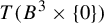 $T(B^3\times \{0\})$
. Identifying
 $B^3$
with
 $B^3\times \{0\}$
, one can see that
 $\widetilde {\mathcal {N}}_{B(\Lambda )}$
admits an invariant splitting
 $\mathcal {N}^{ss}\oplus \mathcal {N}^I\oplus \mathcal {N}_2$
, where
 $\mathcal {N}^{ss}$
and
 $\mathcal {N}_2$
are given by the splitting
 $\widetilde {\mathcal {N}}(B(\Lambda _0))=\mathcal {N}^{ss}\oplus \mathcal {N}_2$
and
 $\mathcal {N}^I={\mathbb R}^I$
. We need to prove that this splitting is dominated. Following [Reference Mañé38], it suffices to show that for any ergodic invariant measure supported on
 $B(\Lambda )$
, the Lyapunov exponents corresponding to the three subbundles satisfy
 $$ \begin{align} \eta^{ss}<\eta^{I}<\eta_2. \end{align} $$
Recall from the construction that there is a dominated splitting
 $T_{\sigma }\Omega =E^{ss}\oplus {\mathbb R}^I\oplus E^c\oplus E^u$
such that the corresponding Lyapunov exponents of the subbundles are
 $$ \begin{align*}\unicode{x3bb}^s<-\theta<\unicode{x3bb}^c<\unicode{x3bb}^u.\end{align*} $$
Moreover, we have defined
 $\unicode{x3bb} ^s_0=\log \|D\Phi _1^{X^0}|_{E^{ss}_{\Lambda _0}}\|$
which satisfies
 $\unicode{x3bb} ^s\leq \unicode{x3bb} ^s_0<-\theta $
. See §3.2.
Let
 $\mu $
be any ergodic invariant measure supported on
 $B(\Lambda )$
. Suppose
 $\beta _*\mu $
is the Dirac measure at
 $\sigma $
, then
 $\mu $
is the Dirac measure supported either on
 $\langle E^c_{\sigma }\rangle $
or on
 $\langle E^u_{\sigma }\rangle $
. In both cases, we have
 $$ \begin{align*}\eta^{ss}=\unicode{x3bb}^s < -\theta=\eta^{I}.\end{align*} $$
Then, we show that
 $\eta ^{I}<\eta _2$
as follows: if
 $\mu $
is the Dirac measure on
 $\langle E^c_{\sigma }\rangle $
, then
 $\eta _2=\unicode{x3bb} ^u$
; otherwise,
 $\mu $
is the Dirac measure on
 $\langle E^u_{\sigma }\rangle $
, then
 $\eta _2=\unicode{x3bb} ^c$
. In both cases, it follows from (3.3) that
 $$ \begin{align*}\eta^{I}=-\theta<\unicode{x3bb}^c\leq \eta_2.\end{align*} $$
Hence, (4.1) holds when
 $\beta _*\mu $
is the Dirac measure at
 $\sigma $
.
Now, suppose
 $\beta _*\mu $
is not the Dirac measure at
 $\sigma $
, then it is a non-singular ergodic measure for the flow
 $\phi _t^X$
. Since the bundle
 $\mathcal {N}^{ss}$
is obtained from
 $E^{ss}$
by orthogonal projection, the Lyapunov exponent along
 $\mathcal {N}^{ss}$
is no larger than
 $\log \|D\Phi _1^{X^0}|_{E^{ss}_{\Lambda _0}}\|=\unicode{x3bb} ^s_0$
, that is,
 $$ \begin{align*}\eta^{ss}\leq \unicode{x3bb}^s_0.\end{align*} $$
By construction of the example, on every point
 $(x,0)\in \Lambda $
, it holds
 $$ \begin{align*} -\theta\leq \frac{\partial \zeta(x,s)}{\partial s}\bigg|_{s=0}\leq 0,\end{align*} $$
where
 $\zeta (x,s)=-\theta s(1-\eta (x,s))$
is the last component of
 $X(x,s)$
. This implies that
 $-\theta \leq \eta ^{I}\leq 0$
. Then, by the inequality (3.3), one has
 $$ \begin{align*}\eta^{ss}\leq \unicode{x3bb}^s_0<-\theta\leq \eta^I\leq 0.\end{align*} $$
Since
 $E^{cu}$
is sectionally expanding and
 $\mathcal {N}_2$
is obtained from
 $E^{cu}$
by intersecting with the normal bundle, one deduces that the Lyapunov exponent along
 $\mathcal {N}_2$
is larger than zero, that is,
 $\eta _2>0$
. Therefore, (4.1) also holds in this case. This finishes the proof of the lemma.
Remark 4.4. From the proof, we can see that
 $E^{cu}_{\Lambda }=\beta _*(\mathcal {F}(\Lambda )\oplus \mathcal {N}_2)$
, where the map
 $\beta _*$
takes each vector
 $(l,v)\in \beta ^*(TM)$
to
 $v\in TM$
.
Proof of Proposition 3.2
By Lemmas 4.2 and 4.3, the extended normal bundle
 $\widetilde {\mathcal {N}}_{\mathcal {F}(\Lambda )}$
admits a dominated splitting with one-dimensional subbundles. Then, it follows from Lemma 2.5 that any fundamental sequence of
 $\Lambda $
admits an index i dominated splitting, for
 $i=1$
and
 $i=2$
. Thus Lemma 4.1 shows that
 $X|_{\Lambda }$
is locally away from homoclinic tangencies.
5 Existence of sectionally expanding subbundle: proof of Proposition 3.3
By construction, the chain recurrence class
 $\Lambda $
admits a two-dimensional invariant bundle
 $E^{cu}\subset T_{\Lambda }\Omega $
which is sectionally expanding for
 $\Phi ^X_t$
. Proposition 3.3 asserts that this property also holds for nearby chain recurrence classes for
 $C^1$
perturbations.
This section gives a proof of Proposition 3.3. For this purpose, we turn to the dominated splitting
 $\widetilde {\mathcal {N}}_{\mathcal {F}(\Lambda )}=\mathcal {N}_1\oplus \mathcal {N}_2$
given by Proposition 3.2, where
 $\mathcal {N}_1=\mathcal {N}^{ss}\oplus \mathcal {N}^I$
. As in Remark 4.4, we have
 $E^{cu}_{\Lambda }=\beta _*(\mathcal {F}(\Lambda )\oplus \mathcal {N}_2)$
, which is a two-dimensional sectionally expanding subbundle for the tangent flow.
Definition 5.1. Let
 $\mathcal {E}\subset \beta ^*(TM)$
be any invariant bundle for the extended tangent flow
 $\tilde {\Phi }_t$
. We say that the bundle
 $\mathcal {E}$
projects to a continuous bundle
 $E\subset TM$
if E is continuous and for any
 $l\in \iota (\mathcal {E})$
, it holds
 $\beta _*(\mathcal {E}_l)=E_{\beta (l)}$
.
Remark 5.2. If
 $\mathcal {E}$
is continuous and it satisfies
 $\beta _*(\mathcal {E}_{l_1})=\beta _*(\mathcal {E}_{l_2})$
for any
 $l_1,l_2\in \iota (\mathcal {E})$
with
 $\beta (l_1)=\beta (l_2)$
, then
 $E=\beta _*(\mathcal {E})$
is a well-defined continuous subbundle of
 $TM$
. Moreover, it is easy to see that E is invariant for the tangent flow
 $\Phi _t$
if
 $\mathcal {E}$
is invariant for the extended tangent flow
 $\tilde {\Phi }_t$
.
Proposition 3.3 will be proved as a corollary of the following result, which is stated in a slightly more general setting.
Proposition 5.3. Let
 $C_X$
be a chain recurrence class of a vector field
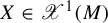 $X\in \mathscr {X}^1(M)$
such that every singularity in the class, say
 $\rho $
, is Lorenz-like with stable index
 $i_0$
(
 $1<i_0<\operatorname {dim} M$
) and
 $C_X\cap (W^{ss}(\rho ,X)\setminus \{\rho \})=\emptyset $
. Suppose
 $\widetilde {\mathcal {N}}_{\mathcal {F}(C_X)}$
admits a dominated splitting
 $\mathcal {N}_1\oplus \mathcal {N}_2$
such that
 $\operatorname {dim} \mathcal {N}_1=i_0-1$
. Then, there is a neighborhood U of
 $C_X$
and a neighborhood
 $\mathcal {U}$
of X such that for any
 $Y\in \mathcal {U}$
and any chain recurrence class
 $C_{Y}\subset U$
of Y, the class admits a dominated splitting
 $\widetilde {\mathcal {N}}_{\mathcal {F}(C_Y)}=\mathcal {N}^Y_1\oplus \mathcal {N}^Y_2$
such that
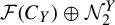 $\mathcal {F}(C_Y)\oplus \mathcal {N}^Y_2$
projects to a continuous bundle
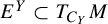 $E^Y\subset T_{C_Y}M$
with
 $\operatorname {dim} E^Y=\operatorname {dim} M-i_0+1$
.
Proof. By robustness of dominated splitting, there exist a neighborhood
 $\mathcal {B}$
of
 $\mathcal {F}(C_X)$
and a neighborhood
 $\mathcal {U}$
of X such that for any
 $Y\in \mathcal {U}$
and for any invariant set
 $\Delta \subset \mathcal {B}$
of the extended tangent flow of Y, the normal bundle
 $\widetilde {\mathcal {N}}(\Delta )$
admits a dominated splitting
 $\mathcal {N}^Y_1\oplus \mathcal {N}^Y_2$
with respect to the extended linear Poincaré flow
 $\tilde {\psi }_t^{Y}$
, and it satisfies
 $\operatorname {dim} \mathcal {N}^Y_1= i_0-1$
. By Lemma 2.2, there exists a neighborhood U of
 $C_X$
such that for any
 $Y\in \mathcal {U}$
(shrinking
 $\mathcal {U}$
if necessary), for any chain recurrence class
 $C_{Y}\subset U$
, one has
 $\mathcal {F}(C_{Y})\subset \mathcal {B}$
. Hence, there is a dominated splitting
 $\widetilde {\mathcal {N}}_{\mathcal {F}(C_{Y})}=\mathcal {N}^Y_1\oplus \mathcal {N}^Y_2$
with index
 $i_0-1$
, that is,
 $\operatorname {dim} \mathcal {N}^Y_1=i_0-1$
.
Since the singularities in
 $C_X$
are all Lorenz-like, by reducing U and
 $\mathcal {U}$
, we can assume that singularities in
 $C_Y$
are also Lorenz-like. In particular, for any singularity
 $\rho \in C_Y$
, there is a dominated splitting
 $T_{\rho }M=E^{ss}_{\rho }\oplus E^{cu}_{\rho }$
such that
 $\operatorname {dim} E^{ss}_{\rho }=i_0-1$
. Moreover, by Lemma 2.3, we can assume that for any
 $l\in \mathcal {F}(C_Y)$
, if
 $\beta (l)=\rho $
is a singularity, then
 $l\in E^{cu}_{\rho }$
. As the dominated splitting
 $\widetilde {\mathcal {N}}_{\mathcal {F}(C_{Y})}=\mathcal {N}^Y_1\oplus \mathcal {N}^Y_2$
has index
 $i_0-1$
, which equals to
 $\operatorname {dim} E^{ss}_{\rho }$
, the uniqueness of domination implies that
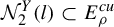 $\mathcal {N}^Y_2(l)\subset E^{cu}_{\rho }$
and hence
 $\beta _*(l\oplus \mathcal {N}^Y_2(l))=E^{cu}_{\rho }$
. Note that the subspace
 $E^{cu}_{\rho }$
is unique for all
 $l\in \mathcal {F}(C_Y)\cap \beta ^{-1}(\rho )$
. For any
 $l\in \mathcal {F}(C_Y)$
with
 $\beta (l)=x$
a regular point, we have
 $l=l^Y_x$
. Thus, we can define
 $E^{cu}_x=\beta _*(l\oplus \mathcal {N}_2(l))$
. In this way, we define a bundle
 $E^{cu}$
over
 $C_Y$
. By continuity of the map
 $\beta _*$
and the bundle
 $\mathcal {N}^Y_2$
, one can see that the bundle
 $E^{cu}$
is continuous at regular points. For any singularity
 $\rho \in C_Y$
, let
 $x_n$
be a sequence in
 $C_Y$
such that
 $x_n\to \rho $
and
 $l_n=l^Y_{x_n}\to l$
. We have
 $$ \begin{align*}E^{cu}_{x_n}=\beta_*(l_n\oplus \mathcal{N}_2^Y(l_n))\to \beta_*(l\oplus\mathcal{N}_2^Y(l))=E^{cu}_{\rho}.\end{align*} $$
Hence,
 $E^{cu}$
is also continuous at
 $\rho $
. Therefore,
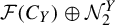 $\mathcal {F}(C_Y)\oplus \mathcal {N}^Y_2$
projects to the continuous bundle
 $E^{cu}$
with
 $\operatorname {dim} E^{cu}=\operatorname {dim} M-i_0+1$
.
Proof of Proposition 3.3
Let
 $\widetilde {\mathcal {N}}_{\mathcal {F}(\Lambda )}=\mathcal {N}_1\oplus \mathcal {N}_2$
with
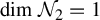 $\operatorname {dim} \mathcal {N}_2=1$
be the dominated splitting given by Proposition 3.2. Then,
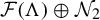 $\mathcal {F}(\Lambda )\oplus \mathcal {N}_2$
projects to the two-dimensional continuous bundle
 $E^{cu}_{\Lambda }$
, which is sectionally expanded. The neighborhoods
 $U\subset U_{\Lambda }$
of
 $\Lambda $
and
 $\mathcal {U}$
of X are given by Proposition 5.3. By reducing these neighborhoods, we can assume that for any
 $Y\in \mathcal {U}$
and any chain recurrence class
 $C_Y\subset U$
, the splitting
 $\widetilde {\mathcal {N}}_{\mathcal {F}(C_Y)}=\mathcal {N}^Y_1\oplus \mathcal {N}^Y_2$
is close enough to
 $\widetilde {\mathcal {N}}_{\mathcal {F}(\Lambda )}=\mathcal {N}_1\oplus \mathcal {N}_2$
. This implies that
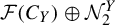 $\mathcal {F}(C_Y)\oplus \mathcal {N}^Y_2$
projects to a continuous bundle
 $E^Y$
that is close enough to
 $E^{cu}_{\Lambda }$
; hence, is also sectionally expanded. Moreover, as
 $E^Y$
contains
 $\beta _*(\mathcal {F}(C_Y))$
, it contains
 $Y(x)$
for all
 $x\in C_Y$
.
We now consider the case when
 $C_Y=C(\sigma _Y,Y)$
. For any
 $Y_n\to Y$
in the
 $C^1$
topology, Lemma 2.2 and the upper semi-continuity of chain recurrence classes imply that the upper limit of
 $\mathcal {F}(C(\sigma _{Y_n},Y_n))$
is a compact subset of
 $\mathcal {F}(C_Y)$
. Note that
 $E^Y=\beta _*(\mathcal {F}(C_Y)\oplus \mathcal {N}_2^Y)$
. By robustness of the dominated splitting
 $\widetilde {\mathcal {N}}_{\mathcal {F}(C_Y)}=\mathcal {N}^Y_1\oplus \mathcal {N}^Y_2$
, the subbundle
 $\mathcal {N}^Y_2$
varies continuously with respect to Y in the following sense: let
 $l_n\to l\in \mathcal {F}(C_Y)$
such that
 $l_n\in \mathcal {F}(C(\sigma _{Y_n},Y_n))$
with
 $Y_n\to Y$
in the
 $C^1$
topology, then
 $\mathcal {N}_2^{Y_n}(l_n)\to \mathcal {N}_2^Y(l)$
. As the projection
 $\beta _*$
is continuous, we conclude that
 $$ \begin{align} E^{Y_n}(\beta(l_n))=\beta_*(l_n\oplus\mathcal{N}^{Y_n}_2(l_n))\to E^Y(\beta(l)) \end{align} $$
in the topology of the tangent bundle. Now, let
 $x_n\in C(\sigma _{Y_n},Y_n)$
be any sequence such that
 $x_n\to x\in C_Y$
. If x is a regular point, we can assume without loss of generality that
 $x_n$
are all regular and take
 $l_n=l^{Y_n}_{x_n}$
, then
 $l_n\to l=l^Y_x\in \mathcal {F}(C_Y)$
. By (5.1), we have
 $E^{Y_n}(x_n)\to E^Y(x)$
. If x is a singularity, that is,
 $x=\sigma _Y$
, to prove the convergence
 $E^{Y_n}(x_n)\to E^Y(x)$
, we need only show that every convergent subsequence of
 $\{E^{Y_n}(x_n)\}$
has the same limit
 $E^Y(x)$
. Without loss of generality, we assume that
 $\{E^{Y_n}(x_n)\}$
itself is convergent. For each n, let
 $l_n\in \mathcal {F}(C(\sigma _{Y_n},Y_n))$
such that
 $\beta (l_n)=x_n$
. We can take a subsequence
 $\{l_{n_k}\}$
such that
 $l_{n_k}\to l\in \mathcal {F}(C_Y)$
with
 $\beta (l)=x$
. By (5.1), we have
 $E^{Y_{n_k}}(x_{n_k})\to E^Y(x)$
. Consequently, as
 $\{E^{Y_n}(x_n)\}$
is convergent, its limit is
 $E^Y(x)$
. This completes the proof of Proposition 3.3.
In the case where
 $C_Y$
is non-singular, the sectional expanding property of the
 $E^Y$
bundle implies that the normal bundle
 $\mathcal {N}^Y_2$
is expanded. This also holds for any non-singular compact invariant set in U.
Corollary 5.4. Let the neighborhoods U and
 $\mathcal {U}$
be given by Proposition 3.3. For any
 $Y\in \mathcal {U}$
and any compact
 $\phi ^Y_t$
-invariant set
 $\Lambda _Y\subset U$
such that
 $\Lambda _Y\cap \operatorname {Sing}(Y)=\emptyset $
, the normal bundle
 $\mathcal {N}_{\Lambda _Y}$
admits a dominated splitting
 $\mathcal {N}_1\oplus \mathcal {N}_2$
such that
 $\mathcal {N}_2$
is one-dimensional and expanded.
6 Uniqueness of Lyapunov stable class: proof of Proposition 3.4
In this section, we prove Proposition 3.4. In other words, we show that for
 $C^1$
perturbations of the vector field X, any Lyapunov stable chain recurrence class in a small neighborhood of
 $\Lambda $
contains the singularity
 $\sigma $
and the periodic orbit Q. We shall make use of the sectional expanding property of the
 $E^{cu}$
subbundle in the splitting
 $T_{\Lambda }\Omega =E^{ss}\oplus E^{cu}\oplus {\mathbb R}^I$
. The difficulty lies in the fact that
 $E^{cu}$
is tangled: there is no domination between the subbundles
 $E^{cu}$
and
 ${\mathbb R}^I$
. As a bypass, we will consider the dominated splitting
 $\widetilde {\mathcal {N}}_{\mathcal {F}(\Lambda )}=\mathcal {N}_1\oplus \mathcal {N}_2$
given by Proposition 3.2, where
 $\mathcal {N}_1=\mathcal {N}^{ss}\oplus \mathcal {N}^I$
.
The rough idea for the proof of Proposition 3.4 goes as follows. We will first extend the dominated splitting
 $\widetilde {\mathcal {N}}_{\mathcal {F}(\Lambda )}=\mathcal {N}_1\oplus \mathcal {N}_2$
to a neighborhood
 $\mathcal {B}_0$
of
 $\mathcal {F}(\Lambda )$
and define a cone around
 $\mathcal {N}_2$
on the normal bundle (§6.1). Then, we use the cone on the normal bundle to construct an invariant cone on the cross-section
 $\Sigma $
for the first return map and show that vectors in the cone on
 $\Sigma $
are expanded by the first return map (§§6.2 and 6.3). Finally, we finish the proof of the proposition by an analysis of the first return map (§6.4).
6.1 Dominated splitting and cone field on the normal bundle
For simplicity, we assume that for the dominated splitting
 $\widetilde {\mathcal {N}}_{\mathcal {F}(\Lambda )}=\mathcal {N}_1\oplus \mathcal {N}_2$
, the domination constant
 $T=1$
. In other words,
 $$ \begin{align*} \|\tilde{\psi}_t|_{\mathcal{N}_1(l)}\|\cdot\|\tilde{\psi}_{-t}|_{\mathcal{N}_2(l_t)} \|<\tfrac{1}{2}\quad\text{for all } t\geq 1, \end{align*} $$
where
 $l_t=\hat {\Phi }_t(l)$
. We extend the splitting
 $\widetilde {\mathcal {N}}_{\mathcal {F}(\Lambda )}=\mathcal {N}_1\oplus \mathcal {N}_2$
to a neighborhood
 $\mathcal {B}_0$
of
 $\mathcal {F}(\Lambda )$
in a continuous way. Define on
 $\mathcal {B}_0$
a cone field
 $\mathcal {C}_{\alpha }$
on the normal bundle around the
 $\mathcal {N}_2$
subbundle for any
 $\alpha>0$
:
 $$ \begin{align*}\mathcal{C}_{\alpha}=\{v=v_1+v_2\in\mathcal{N}_{\mathcal{B}_0}: v_1\in\mathcal{N}_1, v_2\in \mathcal{N}_2, \|v_1\|\leq\alpha\|v_2\|\}.\end{align*} $$
We define also the cone
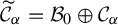 $\widetilde {\mathcal {C}}_{\alpha }=\mathcal {B}_0\oplus \mathcal {C}_{\alpha }$
. (Technically,
 $\widetilde {\mathcal {C}}_{\alpha }$
is not a cone, but a ‘wedge’.) In other words,
 $v\in \widetilde {\mathcal {C}}_{\alpha }$
if and only if there is a decomposition
 $v=v_1+v_2$
such that
 $v_1\in \mathcal {B}_0$
and
 $v_2\in \mathcal {C}_{\alpha }$
. By domination of the splitting
 $\mathcal {N}_1\oplus \mathcal {N}_2$
and continuity, we have the following lemma.
Lemma 6.1. For any
 $\alpha>0$
, there exist a neighborhood
 $\mathcal {U}$
of X and a neighborhood
 $\mathcal {B}\subset \mathcal {B}_0$
of
 $\mathcal {F}(\Lambda )$
such that for any any
 $Y\in \mathcal {U}$
and
 $l\in \mathcal {B}$
, if
 $\hat {\Phi }^Y_{[0,t]}(l)\subset \mathcal {B}$
with
 $t\geq 1$
, then
 $$ \begin{align*}\tilde{\psi}^Y_t(\mathcal{C}_{\alpha}(l))\subset\mathcal{C}_{\alpha/2}(\hat{\Phi}^Y_t(l)) \quad \text{and}\quad \tilde{\Phi}^Y_t(\widetilde{\mathcal{C}}_{\alpha}(l))\subset\widetilde{\mathcal{C}}_{\alpha/2}(\hat{\Phi}^Y_t(l)).\end{align*} $$
Note that the vector bundle
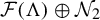 $\mathcal {F}(\Lambda )\oplus \mathcal {N}_2$
is invariant for the extended tangent flow
 $\tilde {\Phi }_t$
. By Remark 4.4,
 $\beta _*(\mathcal {F}(\Lambda )\oplus \mathcal {N}_2)=E^{cu}_{\Lambda }$
, which is sectionally expanded by the tangent flow. Following from the continuity of the map
 $\beta _*$
and by reducing
 $\mathcal {B}_0$
, we can fix
 $\alpha _0>0$
small and a neighborhood
 $\mathcal {U}_0$
of X such that for any
 $Y\in \mathcal {U}_0$
and
 $l\in \mathcal {B}_0$
, if
 $\hat {\Phi }^Y_{[0,t]}(l)\subset \mathcal {B}_0$
with
 $t\geq 1$
, then for any two-dimensional subspace
 $\mathcal {P}\subset \widetilde {\mathcal {C}}_{\alpha _0}(l)$
, the projection
 $\beta _*(\mathcal {P})$
is close enough to
 $E^{cu}_{\Lambda }$
and hence,
 $$ \begin{align} |\!\det(\Phi^Y_t|_{\beta_*(\mathcal{P})})|>e^{\gamma t/2}, \end{align} $$
where
 $\gamma>0$
is given as in (3.1).
We assume that the results of Lemma 6.1 hold for the fixed
 $\alpha =\alpha _0$
with
 $\mathcal {U}=\mathcal {U}_0$
and
 $\mathcal {B}=\mathcal {B}_0$
. Moreover, by Lemma 2.3, we assume that
 $$ \begin{align} W^{ss}(\sigma_Y,Y)\cap C(\sigma_Y,Y)=\{\sigma_Y\} \quad \text{for any } Y\in\mathcal{U}_0, \end{align} $$
where
 $W^{ss}(\sigma _Y,Y)$
is the strong stable manifold of
 $\sigma _Y$
tangent to
 $E^{ss}_{\sigma }\oplus {\mathbb R}^I$
.
6.2 A forward invariance of
$\mathcal {B}_0$

Recall that there is a cross-section
 $\Sigma =\Sigma _0\times I$
of the flow
 $\phi ^X_t$
. One can see that
 $\Sigma $
remains a cross-section for vector fields close to X. In this section, we prove the following lemma.
Lemma 6.2. There exist a neighborhood
 $U_1$
of
 $\Lambda $
and a
 $C^1$
neighborhood
 $\mathcal {U}_1$
of X such that for any
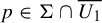 $p\in \Sigma \cap \overline {U_1}$
, for any
 $Y\in \mathcal {U}_1$
and
 $t\geq 0$
, it holds
 $l^Y_{p_t}\in \mathcal {B}_0$
, where
 $p_t=\phi ^Y_t(p)$
.
For the proof of Lemma 6.2, we need to consider orbit segments arbitrarily close to the singularity. Note that the tangent space at the singularity
 $\sigma $
admits a dominated splitting
 $T_{\sigma }\Omega =F^{ss}_{\sigma }\oplus E^{cu}_{\sigma }$
, where
 $F^{ss}_{\sigma }=E^{ss}_{\sigma }\oplus {\mathbb R}^I$
; and by construction, it holds
 $\mathcal {F}(\Lambda )\cap T_{\sigma }\Omega =E^{cu}_{\sigma }$
. One defines on
 $T_{\sigma }\Omega $
a
 $cu$
-cone
 $C^{cu}_{\alpha }$
around the
 $E^{cu}_{\sigma }$
bundle. By domination, the cone
 $C^{cu}_{\alpha }$
is forward contracting. We extend the cone continuously to a ball around
 $\sigma $
, which is denoted by
 $W_0$
. Let K be the intersection of
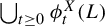 $\bigcup _{t\geq 0}\phi ^X_t(L)$
with
 $\partial W_0$
, which is a compact subset of
 $\partial W_0$
. We assume that the ball
 $W_0$
is small such that
 $W_0\cap \Sigma =\emptyset $
and since the singularity is Lorenz-like, there exists
 $\alpha>0$
such that for any
 $p\in K$
, it holds
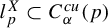 $l^X_p\subset C^{cu}_{\alpha }(p)$
. By reducing
 $\mathcal {U}_0$
if necessary, there exists a neighborhood
 $N_K\subset \partial W_0$
of K such that
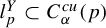 $l^Y_p\subset C^{cu}_{\alpha }(p)$
for any
 $p\in N_K$
and
 $Y\in \mathcal {U}_0$
. Moreover, we assume that the cone
 $C^{cu}_{\alpha }$
is forward contracting under the tangent flow
 $\Phi ^Y_t$
for any
 $Y\in \mathcal {U}_0$
.
Lemma 6.3. There exists a neighborhood
 $W_1\subset W_0$
of
 $\sigma $
and a neighborhood
 $\mathcal {U}_1\subset \mathcal {U}_0$
of X such that for any
 $Y\in \mathcal {U}_1$
, any orbit segment from a point
 $p\in \Sigma $
to a point
 $q\in \overline {W_1}$
crosses
 $N_K$
, and moreover,
 $l^Y_q\in \mathcal {B}_0$
.
Proof. Since
 $\Sigma $
can be a cross-section for any vector field
 $C^1$
close to X and its image under the first return map remains in the interior of
 $\Sigma $
, we need only consider orbit segments from
 $p\in \Sigma $
to
 $q\in \overline {W_1}$
without returns to
 $\Sigma $
. Since
 $N_K$
is a neighborhood of K, there exists a neighborhood
 $W_1\subset W_0$
of
 $\sigma $
such that any orbit segment S of X from a point
 $p\in \Sigma $
to a point
 $q\in \overline {W_1}$
(without returns) crosses
 $N_K$
. Moreover, let r be the intersection of S with
 $N_K$
, then the orbit segment from r to q is contained in
 $\overline {W_0}$
. See Figure 3. Shrinking
 $W_1$
if necessary, there exists a neighborhood
 $\mathcal {U}_1\subset \mathcal {U}_0$
of X such that the same property holds for every
 $Y\in \mathcal {U}_1$
. The following argument shows that
 $l^Y_q\in \mathcal {B}_0$
if we choose
 $W_1$
small enough.
Local analysis around the singularity. Note that the strong stable direction is two-dimensional.

Since
 $E^{cu}_{\sigma }\subset \mathcal {F}(\Lambda )$
and
 $\mathcal {B}_0$
is a neighborhood of
 $\mathcal {F}(\Lambda )$
, we can assume that
 $W_1$
is small enough and there exists a constant
 $\alpha '>0$
such that for any
 $q\in \overline {W_1}$
and non-zero vector
 $v\in T_q\Omega $
, if
 $v\in C^{cu}_{\alpha '}(q)$
, then
 $\langle v\rangle \in \mathcal {B}_0$
; and if the backward orbit of q hits
 $N_K$
at a point r before leaving
 $W_0$
, then the time t from r to q is large enough so that
 $\Phi ^Y_t(C^{cu}_{\alpha }(r))\subset C^{cu}_{\alpha '}(q)$
, by the contracting property of the cone. In particular, since
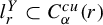 $l^Y_r\subset C^{cu}_{\alpha }(r)$
, we have
 $l^Y_q=\hat {\Phi }^Y_t(l^Y_r)\subset C^{cu}_{\alpha '}(q)$
. It follows that
 $l^Y_q\in \mathcal {B}_0$
.
The next result considers orbit segments away from the singularity.
Lemma 6.4. Reducing
 $\mathcal {U}_1$
if necessary, there exists an attracting neighborhood
 $U_1$
of
 $\Lambda $
such that for any
 $Y\in \mathcal {U}_1$
, one has
 $\phi ^Y_1(\overline {U_1})\subset U_1$
. Moreover, for any
 $p\in \overline {U_1}\setminus W_1$
, it holds that
 $l^{Y}_{p_t}\in \mathcal {B}_0$
for all
 $t\in [0,1]$
, where
 $p_t=\phi ^Y_t(p)$
, and
 $\tilde {\psi }^{Y}_1(\mathcal {C}_{\alpha _0}(l^{Y}_p))\subset \mathcal {C}_{\alpha _0/2}(l^{Y}_{p_1})$
.
Proof. Reducing
 $\mathcal {U}_1$
if necessary, we can take a neighborhood
 $W^{\prime }_1\subset W_1$
of
 $\sigma $
such that for any
 $p\in W^{\prime }_1$
and any
 $Y\in \mathcal {U}_1$
, we have
 $\phi ^Y_t(p)\in W_1$
for all
 $t\in [-1,1]$
. Since
 $\sigma $
is the only singularity in
 $\Lambda $
, we have
 $$ \begin{align} \mathcal{F}(\Lambda)\setminus\beta^{-1}(W^{\prime}_1)=\{l^X_p: p\in \Lambda\setminus W^{\prime}_1\}. \end{align} $$
By construction of the vector field X, there exist arbitrarily small attracting neighborhoods of
 $\Lambda $
. Following from (6.3), we can take an attracting neighborhood
 $U_1$
of
 $\Lambda $
and reduce the neighborhood
 $\mathcal {U}_1$
of X such that
 $\phi ^Y_1(\overline {U_1})\subset U_1$
and
 $l^Y_p\in \mathcal {B}_0$
for any
 $Y\in \mathcal {U}_1$
and for any
 $p\in \overline {U_1}\setminus W^{\prime }_1$
. This implies that for all
 $p\in \overline {U_1}\setminus W_1$
and
 $t\in [0,1]$
, we have
 $l^{Y}_{p_t}\in \mathcal {B}_0$
, and hence by Lemma 6.1,
 $\tilde {\psi }^{Y}_1(\mathcal {C}_{\alpha _0}(l^{Y}_p))\subset \mathcal {C}_{\alpha _0/2}(l^{Y}_{p_1})$
.
We can now finish the proof of Lemma 6.2.
Proof of Lemma 6.2
Let the neighborhoods
 $\mathcal {U}_1$
of X and
 $U_1$
of
 $\Lambda $
be given by Lemmas 6.3 and 6.4. Let p be any point in
 $\Sigma \cap \overline {U_1}$
. By Lemma 6.4,
 $l^Y_{p_t}\in \mathcal {B}_0$
for
 $t\in [0,1]$
. If
 $p_1\in W_1$
, let
 $t_1>1$
be such that the orbit segment
 $\phi ^Y_{[1,t_1]}(p)\subset \overline {W_1}$
and
 $p_{t_1}\in \partial W_1$
. Then, it follows from Lemma 6.3 that
 $l^Y_{p_t}\in \mathcal {B}_0$
for
 $t\in [1,t_1]$
. If
 $p_1\notin W_1$
, it follows from Lemma 6.4 again that
 $l^Y_{p_t}\in \mathcal {B}_0$
for any
 $t\in [1,2]$
. Inductively, one concludes that
 $l^Y_{p_t}\in \mathcal {B}_0$
for all
 $t\geq 0$
.
6.3 Invariant cone on the cross-section and expanding property
Recall that
 $R:\Sigma \setminus L\to \Sigma $
is the first return map, where L is the intersection of the local stable manifold of
 $\sigma $
with
 $\Sigma $
(§3.2). For any
 $Y\in \mathcal {U}_1$
, let
 $L_Y=W^s_{\mathrm {loc}}(\sigma _Y,Y)\cap \Sigma $
and
 $R^Y:\Sigma \setminus L_Y\to \Sigma $
be the first return map. Let
 $TR^Y$
be the tangent map of
 $R^Y$
. For simplicity, let us denote
 $$ \begin{align*}\Sigma^*=\Sigma\cap \overline{U_1}.\end{align*} $$
We define in this section a cone on
 $\Sigma ^*$
such that it is invariant under
 $TR^Y$
and moreover, vectors in the cone will be shown to be expanded by
 $TR^Y$
. This allows us to consider curves tangent to the cone on
 $\Sigma ^*$
and show that the length of such curves increase under the iteration of the first return map.
In the following, for any
 $0<\alpha \leq \alpha _0$
and
 $p\in \overline {U_1}\setminus \{\sigma _Y\}$
such that
 $l^Y_p\in \mathcal {B}_0$
, we denote
 $\mathcal {C}^Y_{\alpha }(p)=\beta _*(\widetilde {\mathcal {C}}_{\alpha }(l^Y_p))$
, which is a cone on the tangent space
 $T_p\Omega $
. We then define a cone field
 $\mathcal {D}^Y_{\alpha }$
on
 $\Sigma ^*$
by letting
 $\mathcal {D}^Y_{\alpha }(p)=\mathcal {C}^Y_{\alpha }(p)\cap T_p\Sigma $
. By shrinking
 $U_1$
and
 $\mathcal {U}_1$
, the following result holds.
Lemma 6.5. There exist
 $0<\alpha _1<\alpha _0$
and
 $\unicode{x3bb}>1$
such that for any
 $Y\in \mathcal {U}_1$
, any
 $p\in \Sigma ^*\setminus L_Y$
, and any
 $v\in \mathcal {D}^X_{\alpha _1}(p)$
, one has
 $TR^Y(v)\in \mathcal {D}^X_{\alpha _1}(p')$
, where
 $p'=R^Y(p)$
. Moreover,
 $\|TR^Y(v)\|\geq \unicode{x3bb} \|v\|$
.
Proof. Note that restricted to
 $\Sigma ^*$
, the cone
 $\mathcal {C}^Y_{\alpha }(p)$
and hence,
 $\mathcal {D}^Y_{\alpha }(p)$
are uniformly continuous with respect to the vector field Y in the
 $C^1$
topology. Let us fix
 $\alpha _1\in (\alpha _0/2,\alpha _0)$
. Then, by reducing
 $\mathcal {U}_1$
, we can assume that for any
 $Y\in \mathcal {U}_1$
, it holds
 $$ \begin{align*}\mathcal{D}^Y_{\alpha_0/2}(p)\subset \mathcal{D}^X_{\alpha_1}(p)\subset \mathcal{D}^Y_{\alpha_0}(p).\end{align*} $$
Also, from Property (C1) in §3.2, we can assume that
 $t_p>2$
for any
 $p\in \Sigma ^*\setminus L_Y$
. Now, for any
 $v\in \mathcal {D}^X_{\alpha _1}(p)\subset \mathcal {D}^Y_{\alpha _0}(p)$
, we have
 $(l^Y_p,v)\in \widetilde {\mathcal {C}}^Y_{\alpha _0}(l^Y_p)$
. From Lemma 6.2, it follows that
 $l^Y_{p_t}\in \mathcal {B}_0$
for all
 $t\geq 0$
. Thus, by Lemma 6.1, we have
 $\widetilde {\Phi }^Y_{t_p}(l^Y_p,v)\in \widetilde {\mathcal {C}}_{\alpha _0/2}(l^Y_{p'})$
, where
 $p'=R^Y(p)$
. Equivalently, we have
 $\Phi ^Y_{t_p}(v)\in \mathcal {C}^Y_{\alpha _0/2}(p')$
. Projecting
 $\Phi ^Y_{t_p}(v)$
to
 $T_{p'}\Sigma $
along
 $l^Y_{p'}$
, we obtain that
 $$ \begin{align*}TR^Y(v)\in \mathcal{D}^Y_{\alpha_0/2}(p')\subset \mathcal{D}^X_{\alpha_1}(p').\end{align*} $$
This establishes the invariance of the cone
 $\mathcal {D}^X_{\alpha _1}$
.
To see that
 $TR^Y$
is expanding on
 $\mathcal {D}^X_{\alpha _1}$
, we shall refer to the sectional expanding property (6.1). Recall that in the construction of the example, we have assumed the vector field
 $X^0$
to be orthogonal to the cross-section
 $\Sigma _0$
and
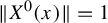 $\|X^0(x)\|=1$
for
 $x\in \Sigma _0$
, see Property (P2) in §3.1. Then, it follows from (3.2) that the vector field X is orthogonal to the cross-section
 $\Sigma $
at points
 $p\in \Sigma _0\times \{0\}$
and
 $\|X(p)\|=1$
. In particular, this holds for
 $p\in \Lambda \cap \Sigma $
. By shrinking
 $U_1$
and
 $\mathcal {U}_1$
if necessary, we can assume that for any
 $Y\in \mathcal {U}_1$
and any
 $p\in \Sigma ^*=\Sigma \cap \overline {U_1}$
,
 $Y(p)$
is almost orthogonal to the cross-section and
 $\|Y(p)\|$
is close to 1. Then, the sectional expanding property (6.1) allows us to obtain a constant
 $\unicode{x3bb}>1$
, independent of Y, such that
 $\|TR^Y(v)\|\geq \unicode{x3bb} \|v\|$
.
The previous result shows that the cone
 $\mathcal {D}^X_{\alpha _1}$
on
 $\Sigma ^*$
is invariant for
 $TR^Y$
, for any
 $Y\in \mathcal {U}_1$
. Moreover,
 $TR^Y$
is expanding on
 $\mathcal {D}^X_{\alpha _1}$
. Note the first return time
 $t_p$
of a point
 $p\in \Sigma ^*\setminus L_Y$
can be arbitrarily large if it is close enough to
 $L_Y$
. In this case, the sectional expanding property (6.1) will guarantee a large expansion rate for
 $TR^Y$
.
Lemma 6.6. There exists a neighborhood
 $N_L$
of L in
 $\Sigma $
such that for any
 $Y\in \mathcal {U}_1$
(reducing
 $\mathcal {U}_1$
if necessary), one has
 $L_Y\subset N_L$
and for any
 $p\in (N_L\setminus L_Y)\cap \Sigma ^*$
,
 $$ \begin{align} \|TR^Y(v)\|>3\|v\|\quad \text{for all } v\in \mathcal{D}^X_{\alpha_1}(p)\setminus\{0\}. \end{align} $$
Proof. By Lemma 6.2 and the sectional expanding property (6.1), there exists
 $t_0>0$
such that for any
 $Y\in \mathcal {U}_1$
and any
 $p\in \Sigma ^*\setminus L_Y$
, if the first return time
 $t_p>t_0$
, then (6.4) holds. By continuity of local stable manifold, for any neighborhood
 $N_L$
of L in
 $\Sigma $
, there exists a
 $C^1$
neighborhood
 $\mathcal {U}$
of X such that for any
 $Y\in \mathcal {U}$
, the intersection
 $L_Y=W^s_{\mathrm {loc}}(\sigma _Y,Y)\cap \Sigma $
is contained in
 $N_L$
. Therefore, by reducing
 $\mathcal {U}_1$
, we can assume that this property holds for
 $Y\in \mathcal {U}_1$
and
 $N_L$
is small enough such that for any
 $p\in (N_L\setminus L_Y)\cap \Sigma ^*$
, the first return time
 $t_p$
is larger than
 $t_0$
. Hence, (6.4) holds.
Definition 6.7. (
$cu$
-curve)

A
 $C^1$
curve J on
 $\Sigma $
is called a cu-curve if it is contained in
 $\Sigma ^*$
and is tangent to the cone
 $\mathcal {D}^X_{\alpha _1}$
.
Lemma 6.8. For any
 $Y\in \mathcal {U}_1$
and any
 $cu$
-curve J such that
 $J\cap L_Y=\emptyset $
, the image
 $R^Y(J)$
remains a
 $cu$
-curve.
Proof. Since
 $J\cap L_Y=\emptyset $
, for any
 $p\in J$
, there is a neighborhood
 $J_p\subset J$
of p and a constant
 $\delta>0$
such that the set
 $\Gamma =\bigcup _{|t-t_p|\leq \delta }\phi ^Y_t(J_p)$
is a two-dimensional submanifold tangent to the cone
 $\mathcal {C}^Y_{\alpha _0}$
, transverse to
 $\Sigma $
. The intersection
 $\Gamma \cap \Sigma $
is contained in
 $\Sigma ^*$
and by Lemma 6.5, is a
 $cu$
-curve. This implies that
 $R^Y(J)$
is a
 $cu$
-curve.
Assuming
 $\mathcal {U}_1$
small enough, the following result holds.
Lemma 6.9. There exists
 ${\varepsilon }_0>0$
such that for any
 $Y\in \mathcal {U}_1$
and any
 $cu$
-curve J, there exists
 $k>0$
such that
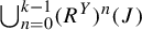 $\bigcup _{n=0}^{k-1} (R^Y)^n(J)$
contains a
 $cu$
-curve with length larger than
 ${\varepsilon }_0$
.
Proof. Assume that the
 $C^1$
neighborhood
 $\mathcal {U}_1$
of X is small enough such that
 $L_Y$
is
 $C^1$
close to L and transverse to
 $\mathcal {D}^X_{\alpha _1}$
with uniform angle. Moreover,
 $N_L$
contains an
 $\varepsilon $
-neighborhood of
 $L_Y$
in
 $\Sigma $
, where
 ${\varepsilon }>0$
is uniform for
 $Y\in \mathcal {U}_1$
. Then, there exists
 ${\varepsilon }_0\in (0,{\varepsilon })$
such that any
 $cu$
-curve with length smaller than
 $\varepsilon _0$
intersects
 $L_Y$
at most once, and moreover, when it does intersect
 $L^Y$
, then it is contained in
 $N_L$
.
Let J be any
 $cu$
-curve that does not intersect
 $L_Y$
. By Lemma 6.8,
 $R^Y(J)$
remains a
 $cu$
-curve. Moreover, Lemma 6.5 shows that
 $\operatorname {len}(R^Y(J))>\unicode{x3bb} \operatorname {len}(J)$
, where
 $\operatorname {len}(\cdot )$
denotes the length of a
 $C^1$
curve. By iteration, the length of
 $(R^Y)^n(J)$
keeps growing if it does not intersect
 $L_Y$
. When
 $(R^Y)^n(J)$
does intersect
 $L_Y$
, then either
 $(R^Y)^n(J)$
has length larger than
 $\varepsilon _0$
, or it is contained in
 $N_L$
and is cut by
 $L_Y$
into two pieces. In the latter case, let
 $J'$
be the longer piece. Then, Lemma 6.6 implies that
 $R^Y(J')$
has length larger than
 $3/2$
times the length of
 $(R^Y)^n(J)$
. The conclusion of the lemma holds by induction.
6.4 Proof of Proposition 3.4
We now fix the neighborhoods
 $U_1$
and
 $\mathcal {U}_1$
small enough so that all the results in §§6.2 and 6.3 hold.
Recall that there is a periodic orbit Q in
 $\Lambda $
with stable index 2 such that its stable manifold is dense in
 $U_{\Lambda }$
, see Property (C2) in §3.2. In particular, the stable manifold of Q intersects
 $\Sigma $
along a dense family of two-dimensional
 $C^1$
disks of the form
 $\mathcal {F}^s(x)\times I$
. It is easy to see that the foliation
 $\mathcal {F}^s\times I$
is transverse to the bundle
 $E^{cu}$
, so we can assume that
 $\alpha _0$
is small such that
 $\mathcal {F}^s\times I$
is transverse to the cone
 $\mathcal {D}^X_{\alpha _0}$
. This implies in particular that any
 $cu$
-curve is transverse to the foliation
 $\mathcal {F}^s\times I$
and the angle between them is uniformly bounded below. By continuity of local stable manifold, there exists a
 $C^1$
neighborhood
 $\mathcal {U}_2$
of X such that for any
 $Y\in \mathcal {U}_2$
, any
 $cu$
-curve with length
 ${\varepsilon }_0$
intersects the stable manifold
 $W^s(Q_Y,Y)$
, where
 ${\varepsilon }_0>0$
is given by Lemma 6.9 and
 $Q_Y$
is the continuation of Q.
Lemma 6.10. For any
 $Y\in \mathcal {U}_1\cap \mathcal {U}_2$
, for any
 $\phi ^Y_t$
-invariant compact set
 $\Gamma \subset U_1$
such that
 $\Gamma \cap \operatorname {Sing}(Y)=\emptyset $
, it holds
 $W^u(\Gamma ,Y)\cap W^s(Q_Y,Y)\neq \emptyset $
and
 $W^u(\Gamma ,Y)\cap W^s(\sigma _Y,Y)\neq~\emptyset $
.
Proof. By Corollary 5.4, there is a dominated splitting
 $\mathcal {N}_{\Gamma }=\mathcal {N}_1\oplus \mathcal {N}_2$
such that
 $\mathcal {N}_2$
is one-dimensional and expanding. This implies that
 $\Gamma $
has an unstable manifold tangent to
 $\langle Y\rangle \oplus \mathcal {N}_2$
. By Lemma 6.1, the cone
 $\mathcal {D}^X_{\alpha _1}$
is invariant under
 $TR^Y$
, which implies that
 $(l^Y_p\oplus \mathcal {N}_2(p))\cap T_p\Sigma \subset \mathcal {D}^X_{\alpha _1}(p)$
for any
 $p\in \Gamma \cap \Sigma $
. Then, the intersection of the unstable manifold of
 $\operatorname {Orb}(p)$
with
 $\Sigma $
contains a
 $cu$
-curve J. It follows from Lemma 6.9 that the length of J can be assumed to be larger than
 ${\varepsilon }_0$
. Since
 $Y\in \mathcal {U}_2$
,
 $J\cap W^s(Q_Y,Y)\neq \emptyset $
. Hence,
 $W^u(\Gamma ,Y)\cap W^s(Q_Y,Y)\neq \emptyset $
.
For the proof of
 $W^u(\Gamma ,Y)\cap W^s(\sigma _Y,Y)\neq \emptyset $
, we need only show that
 $W^u(\Gamma ,Y)\cap L_Y\neq \emptyset $
. Assume that J does not intersect
 $L_Y$
, then by invariance of the cone
 $\mathcal {D}^X_{\alpha _1}$
and Lemma 6.5, the iterate
 $R^Y(J)$
remains a
 $cu$
-curve with length larger than
 $\unicode{x3bb} \operatorname {len}(J)$
. By iteration, the length of
 $(R^Y)^n(J)$
keeps growing if the first
 $n-1$
iterates do not intersect with
 $L_Y$
. As the cone
 $\mathcal {D}^X_{\alpha _1}$
is transverse to
 $\mathcal {F}^s\times I$
, there exists a finite upper bound for the length of
 $cu$
-curves. Hence, there exists
 $n>0$
such that
 $(R^Y)^n(J)\cap L_Y\neq \emptyset $
. Therefore,
 $W^u(\Gamma ,Y)\cap L_Y\neq \emptyset $
.
Corollary 6.11. For any
 $Y\in \mathcal {U}_1\cap \mathcal {U}_2$
, the chain recurrence class
 $C(\sigma _Y,Y)$
is the only Lyapunov stable one contained in
 $U_1$
.
Proof. Let
 $C_Y$
be any Lyapunov stable chain recurrence class of Y contained in
 $U_1$
. Suppose that
 $C_Y$
does not contain the singularity
 $\sigma _Y$
. Then,
 $C_Y$
is non-singular. By Lemma 6.10, we have
 $W^u(C_Y,Y)\cap W^s(\sigma _Y,Y)\neq \emptyset $
. By Lyapunov stability of the chain recurrence class
 $C_Y$
, one would obtain that
 $\sigma _Y\in \mathrm {Cl}(W^u(C_Y,Y))\subset C_Y$
, which is a contradiction. Thus,
 $C_Y$
contains
 $\sigma _Y$
. It follows that
 $C(\sigma _Y,Y)$
is the only Lyapunov stable chain recurrence class in
 $U_1$
.
Let
 $Y\in \mathcal {U}_1\cap \mathcal {U}_2$
. We need to show that
 $Q_Y$
is contained in the Lyapunov stable chain recurrence class
 $C(\sigma _Y,Y)$
. Let us recall the following result in [Reference Gan and Yang27].
Lemma 6.12. [Reference Gan and Yang27, Proposition 4.9]
Let
 $\Delta $
be a compact invariant set of
 $Y\in \mathscr {X}^1(M)$
verifying the following properties.
-
• There exists a dominated splitting
$\mathcal N_{\Delta} = G^{cs} \oplus G^{cu}$
of index
$i$
in the normal bundle of
$\Delta \setminus \operatorname{Sing}(Y)$
with respect to the linear Poincaré flow
$\psi_t$
. -
• Every singularity
$\rho \in \Delta $
is hyperbolic and
$\operatorname {Ind}(\rho )>i$
. Moreover,
$T_\rho M$
admits a partially hyperbolic splitting
$T_{\rho }M=F^{ss}\oplus F^{cu}$
with respect to the tangent flow, where
$\operatorname {dim} F^{ss}=i$
and for the corresponding strong stable manifolds
$W^{ss}(\rho )$
, one has
$W^{ss}(\rho )\cap \Delta =\{\rho \}$
. -
• For every
$x\in \Delta $
, one has
$\omega (x)\cap \mathrm {Sing}(Y)\neq \emptyset $
.







Then, either
 $\Delta $
admits a partially hyperbolic splitting
 $T_\Delta M=E^{ss}\oplus F$
with respect to the tangent flow
 $\Phi ^Y_t$
, where
 $\operatorname {dim} E^{ss}=i$
, or
 $\Delta $
intersects the homoclinic class
 $H(\gamma )$
of a hyperbolic periodic orbit
 $\gamma $
of index i.
Since
 $Y\in \mathcal {U}_1$
, the singularity
 $\sigma _Y$
is Lorenz-like and it follows from Proposition 5.3 that
 $\mathcal {N}_{C(\sigma _Y,Y)}$
admits a dominated splitting
 $\mathcal {N}_1\oplus \mathcal {N}_2$
with index
 $2$
. Moreover, since
 $\mathcal {U}_1\subset \mathcal {U}_0$
and by (6.2), we have
 $W^{ss}(\sigma _Y,Y)\cap C(\sigma _Y,Y)=\{\sigma _Y\}$
. Let us consider the following two cases:
-
(1) either
$\omega (x)\cap \operatorname {Sing}(Y)\neq \emptyset $
for every
$x\in C(\sigma _Y,Y)$
; -
(2) or there exists
$x\in C(\sigma _Y,Y)$
such that
$\omega (x)\cap \operatorname {Sing}(Y)=\emptyset $
, that is,
$\sigma _Y\notin \omega (x)$
.



If Case (1) happens, then all the conditions in Lemma 6.12 are satisfied for
 $C(\sigma _Y,Y)$
. Moreover, the condition in Case (1) implies that
 $C(\sigma _Y,Y)$
cannot contain periodic orbits and hence cannot intersect a homoclinic class. Then, Lemma 6.12 shows that
 $C(\sigma _Y,Y)$
admits a partially hyperbolic splitting
 $T_{C(\sigma _Y,Y)}M=F^{ss}\oplus F^{cu}$
with respect to the tangent flow. One can see that the bundle
 $F^{cu}$
is exactly the sectionally expanding subbundle
 $E^Y$
given by Proposition 3.3. Therefore,
 $C(\sigma _Y,Y)$
is singular hyperbolic and by Corollary 6.11, it is also Lyapunov stable. By the result [Reference Pacifico, Yang and Yang43, Corollary D], the class
 $C(\sigma _Y,Y)$
contains a periodic orbit, which is a contradiction to the assumption that
 $\omega (x)\cap \operatorname {Sing}(Y)\neq \emptyset $
for all
 $x\in C(\sigma _Y,Y)$
. So we are left with Case (2), in which
 $C(\sigma _Y,Y)$
contains a non-singular compact invariant subset
 $\Gamma $
. It follows from Lemma 6.10 that
 ${W^u(\Gamma ,Y)\cap W^s(Q_Y,Y)\neq \emptyset }$
. Then, as
 $\Gamma \subset C(\sigma _Y,Y)$
and
 $C(\sigma _Y,Y)$
is Lyapunov stable (Corollary 6.11), we see that
 $Q_Y\subset C(\sigma _Y,Y)$
.
This ends the proof of Proposition 3.4.