2.1 Experimental set-up

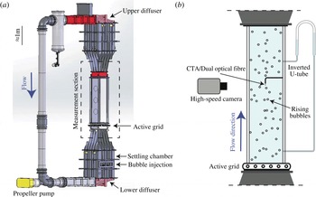
The experiments are performed in the Twente water tunnel, which is a vertical water tunnel as shown in figure 1(a) (Poorte & Biesheuvel Reference Poorte and Biesheuvel2002; Mercado et al. Reference Mercado, Prakash, Tagawa, Sun and Lohse2012; Mathai et al. Reference Mathai, Neut, van der Poel and Sun2016b ). The measurement section is 2 m high, $450~\text{mm}\times 450~\text{mm}$ in cross-section, and made of three glass walls allowing optical access. An upward mean flow passes through an active grid which is positioned below the measurement section (figure 1 b). The active grid generates nearly homogeneous and isotropic turbulence in the measurement section. By varying the rotation speed of the active grid and the liquid mean flow, different turbulence intensities are achieved. Bubbles are injected below the active grid by means of 621 capillary tubes of inner diameter 0.12 mm. The capillaries are mounted on nine islands which are regularly placed in the settling chamber, below the measurement section, in such a way that the bubble distribution is almost homogeneous in the cross-section of measurement. Indeed, the injection location is approximately 3 m below the measurement location. This gives the bubbles enough time to distributed nearly homogeneously in the cross-section. The gas volume fraction is varied from 0.25 % to 0.93 % in this work by changing the gas flow rate. An ascending turbulent bubbly flow, rising at a Reynolds number $Re=V_{r}d/\unicode[STIX]{x1D708}$ (where $V_{r}$ is the relative rising velocity of the bubble, $d$ the mean bubble diameter, and $\unicode[STIX]{x1D708}$ the kinematic viscosity) ranging from 600 to 900 is thus produced.

Figure 1.

(a) The Twente water tunnel facility, where the experiments were performed. (b) A zoomed-in view shows the measurement section with the experimental arrangement used in the present study.

2.2 Instrumentation for the gas-phase characterisation

The gas-phase characterisation consists of measuring the global gas volume fraction, the bubble diameter and the bubble rising velocity. For that purpose, different measurement techniques have been used. The global gas volume fraction $\unicode[STIX]{x1D6FC}$ was measured by using an inverted U-tube (Rensen et al. Reference Rensen, Luther and Lohse2005). We also checked that the global gas volume fraction was comparable to the one measured locally by an optical probe, indicating that the bubble swarm is distributed homogeneously. The diameter and the rising velocity of the bubbles were measured by means of a home-made dual optical fibre probe. The optical fibre probe detects the passage of the bubble interface at two measurement points, which are separated vertically by a distance $\unicode[STIX]{x1D6FF}=3.41$  mm. The bubble velocity is then calculated as $V_{b}=\unicode[STIX]{x1D6FF}/\unicode[STIX]{x0394}t$ , where $\unicode[STIX]{x0394}t$ is the time interval between which one bubble collides successively with each probe. Concerning the diameter, this is estimated from the time during which the leading probe is in the gas phase. More details about the signal processing used can be found in Colombet et al. (Reference Colombet, Legendre, Risso, Cockx and Guiraud2015).

In order to get more details about the gas-phase behaviour, in particular about the aspect ratio of the bubbles, imaging measurements were also performed by using a high-speed camera (Photron FASTCAM SAX2), with a 105 mm macro lens focused at the centre of the measurement section. The recordings were made at an acquisition frequency of 750 frames per second and with an exposure time of $1/14\,035$  s. As the diaphragm of the camera is fully open, the depth of field of the camera is relatively short and was estimated by using a tilted calibration plate. It is around 1 cm. An image-processing method was developed in order to measure the diameter and the velocity of the bubbles. The bubbles are detected by thresholding based on the spatial intensity gradient of the raw images. In order to detect only single bubbles, two criteria were imposed on the detected elements, one on the equivalent diameter $d_{eq}=\sqrt{4A/\unicode[STIX]{x03C0}}$ where $A$ is the area of the detected element, and the other on the solidity. The solidity criterion is given by $A/A_{cv}$ , where $A$ is the area of the region suspected to be the bubble, and $A_{c}$ is the area of the smallest convex polygon engulfing the region of the suspected bubble. Here we used a solidity threshold 0.95, which is comparable to the value used in the literature (Honkanen Reference Honkanen2009).

2.3 Instrumentation for the liquid-phase characterisation

The liquid phase was characterised in the vertical direction only by means of constant temperature anemometry (CTA) for both single-phase and two-phase flow measurements. The CTA probe is located in the middle of the cross-section of measurement, and the signal is acquired at a frequency of 10 KHz for at least 25 min. It is well known that using CTA in a bubbly flow induces disturbances on the velocity measurement when bubbles collide with the CTA probe, generating spurious peaks on the velocity signal. Different methods have been developed to get rid of these spurious peaks and to measure only liquid phase fluctuations (Rensen et al. Reference Rensen, Luther and Lohse2005; van den Berg, Luther & Lohse Reference van den Berg, Luther and Lohse2006; Mercado et al. Reference Mercado, Gomez, Van Gils, Sun and Lohse2010; Prakash et al. Reference Prakash, Mercado, van Wijngaarden, Mancilla, Tagawa, Lohse and Sun2016). In the present study, bubble collisions are detected by thresholding the temporal derivative of the raw velocity signal (Ellingsen et al. Reference Ellingsen, Risso, Roig and Suzanne1997). In fact, the temporal derivative of the velocity signal during a bubble collision is typically well over $150~\text{m}~\text{s}^{-2}$ . For all cases, a velocity derivative of $150~\text{m}~\text{s}^{-2}$ was used. This value is well above any liquid-phase velocity gradient encountered in the water tunnel flow and therefore must occur due to the bubble collisions. Thanks to this operation, the liquid phase is distinguished from the bubble collisions. The mean liquid velocity $U$ , the standard deviation of the velocity fluctuations $u_{rms}$ and the p.d.f. are thus calculated by considering velocity measurements in the liquid phase only. Before calculating the spectrum of the velocity fluctuations, the gas-phase areas of the signal are removed and replaced by linear interpolation. More details about this operation and its consequences may be found in Mercado et al. (Reference Mercado, Gomez, Van Gils, Sun and Lohse2010) and Alméras et al. (Reference Alméras, Cazin, Roig, Risso, Augier and Plais2016).

3.1 Turbulence characterisation

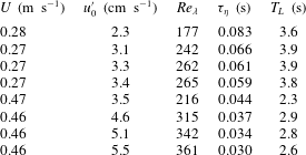
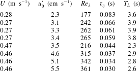
Before investigating turbulent bubbly flows, we will describe the properties of the incident turbulence generated by the active grid. In this study, eight turbulence intensities are investigated, corresponding to two mean flows ( $U=0.27~\text{m}~\text{s}^{-1}$ and $U=0.46~\text{m}~\text{s}^{-1}$ ) and four rotation speeds of the active grid (see table 1). Liquid velocity fluctuations are thus increased from $u_{0}^{\prime }=2.3~\text{cm}~\text{s}^{-1}$ to $u_{0}^{\prime }=5.5~\text{cm}~\text{s}^{-1}$ by increasing the mean flow and/or the rotation speed, allowing us to vary the Taylor–Reynolds number $Re_{\unicode[STIX]{x1D706}}$ from 177 to 361. For the eight cases, the turbulent velocity fluctuations are nearly homogeneous and isotropic, as also seen in previous studies using the same set-up (Mercado et al. Reference Mercado, Gomez, Van Gils, Sun and Lohse2010; Mathai et al. Reference Mathai, Prakash, Brons, Sun and Lohse2015; Prakash et al. 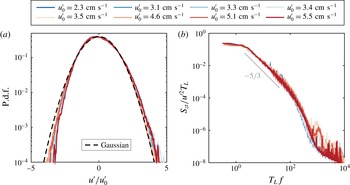Reference Prakash, Mercado, van Wijngaarden, Mancilla, Tagawa, Lohse and Sun2016). In fact, once normalised by the corresponding standard deviation, the p.d.f.s of the velocity fluctuations show a Gaussian behaviour, irrespective of the level of turbulence (figure 2 a). The spectra of the velocity fluctuations present a $-5/3$ scaling over two decades (figure 2 b), within the frequency range $(1/T_{L};1/\unicode[STIX]{x1D70F}_{\unicode[STIX]{x1D702}})$ (table 1), where $T_{L}$ is the integral time scale calculated from the dissipation rate $\unicode[STIX]{x1D716}$ ( $T_{L}=((3/4)C_{0}(\unicode[STIX]{x1D716}/k))^{-1}$ , with $k=3/2u_{0}^{\prime 2}$ , $C_{0}=2.1$ ). The energy dissipation rate $\unicode[STIX]{x1D716}$ is estimated from the second-order longitudinal structure function, which is calculated by means of the Taylor hypothesis, similar to the methods followed in Mathai et al. (Reference Mathai, Prakash, Brons, Sun and Lohse2015, Reference Mathai, Calzavarini, Brons, Sun and Lohse2016a ). The dissipative time scale $\unicode[STIX]{x1D70F}_{\unicode[STIX]{x1D702}}\equiv (\unicode[STIX]{x1D708}/\unicode[STIX]{x1D716})^{1/2}$ is finally estimated for each turbulence level (table 1). It must be noted that the above procedures involve Taylor’s frozen flow hypothesis and the assumption that the second-order structure function $D_{LL}=C_{2}(\unicode[STIX]{x1D716}r)^{2/3}$ (Pope Reference Pope2000). These assumptions are reasonable for the range of parameters in the present study. Typical errors in these estimates lie within 20 %, and have been quantified in prior investigations (Poorte & Biesheuvel Reference Poorte and Biesheuvel2002; Mercado et al. Reference Mercado, Prakash, Tagawa, Sun and Lohse2012).

Figure 2.

Characterisation of the homogeneous isotropic turbulence for different operating conditions (single-phase flow). (a) P.d.f. of the velocity fluctuations normalised by the standard deviation. (b) Normalised spectrum of the velocity fluctuations.

Table 1.

Summary of the flow parameters for single-phase measurements. Here, $U$ is the mean flow velocity, $u_{0}^{\prime }$ is the standard deviation of velocity fluctuations, $Re_{\unicode[STIX]{x1D706}}$ is the Taylor–Reynolds number, and $\unicode[STIX]{x1D70F}_{\unicode[STIX]{x1D702}}$ and $T_{L}$ are the dissipative and integral time scales of the turbulent flow, respectively.

3.2 Bubble properties

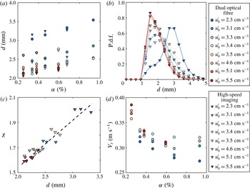
For the eight turbulence levels considered in this study, the gas volume fraction is varied from 0 % to 0.93 % for $U=0.27~\text{m}~\text{s}^{-1}$ and from 0 % to 0.59 % for $U=0.46~\text{m}~\text{s}^{-1}$ . The mean bubble diameter ranges from 2.0 mm to 3.6 mm and depends both on the gas volume fraction and the turbulence level (see figure 3 a). For all levels of turbulence, the mean bubble diameter increases with the gas volume fraction. Moreover, a strong influence of the rotation speed of the active grid on the bubble diameter can be observed: the faster the rotation speed, the smaller are the bubbles. This trend has already been observed by Prakash et al. (Reference Prakash, Mercado, van Wijngaarden, Mancilla, Tagawa, Lohse and Sun2016). The size distributions of the bubbles diameter are presented in figure 3(b) for every level of turbulence at the lowest gas volume fraction investigated. The standard deviation of the bubble diameter is approximately 25–30 % of the mean diameter for all the gas volume fractions and turbulence levels studied. Concerning the aspect ratio of the bubbles, this ranges from 1.6 to 2.0, depending mainly on the rotation speed of the grid and weakly on the gas volume fraction. As shown in figure 3(c) the aspect ratio of the bubble is fully controlled by the bubble diameter: smaller bubbles are more spherical compared to larger ones. The Weber number, $We=\unicode[STIX]{x1D70C}V_{r}^{2}d/\unicode[STIX]{x1D70E}$ in the shown range varies from 1.8 (nearly spherical) to 7.1 (considerably deformed).

Figure 3.

Gas-phase characterisation for different turbulence levels. (a) Mean bubble diameter $d$ as a function of the gas volume fraction $\unicode[STIX]{x1D6FC}$ for different turbulence levels $u_{0}^{\prime }$ . (b) Bubble size distribution for different turbulence levels at the lowest gas volume fraction in our experiments. (c) Aspect ratio $\unicode[STIX]{x1D712}$ of bubbles versus mean bubble diameter $d$ , showing a nearly linear dependence. (d) Relative bubble velocity as a function of the gas volume fraction $\unicode[STIX]{x1D6FC}$ for different turbulence level. The circle symbols denote the measurements made from the dual optical probe, and the triangle symbols denote estimates obtained from high-speed imaging. The colour code reflects the r.m.s. of liquid velocity fluctuations $u_{0}^{\prime }$ of the incident turbulence.

The relative bubble rise velocity $V_{r}$ measured by optical fibre is shown in figure 3(d) as a function of the gas volume fraction for the eight turbulence levels studied. We checked that the relative velocity measured by the dual optical probe was comparable to the one evaluated from the high-speed images (not shown here). The variation between both techniques was within $\pm 5\,\%$ for the moderate volume fractions studied here. The relative rising velocity is calculated as the difference between the measured bubble velocity $V_{b}$ and the liquid mean flow $U$ . Under the present operating conditions, the relative rise velocity ranges from $0.27~\text{m}~\text{s}^{-1}$ to $0.39~\text{m}~\text{s}^{-1}$ and depends both on the turbulence level as well as the gas volume fraction. For any chosen turbulence level the relative rise velocity decreases with the gas volume fraction, as has already been observed for pseudo-turbulence (Riboux et al. Reference Riboux, Risso and Legendre2010; Colombet et al. Reference Colombet, Legendre, Risso, Cockx and Guiraud2015). However, more experiments would be required to have a deeper understanding on the dependence of $V_{r}$ on the gas volume fraction and the turbulence level, which is outside the scope of this study. Nevertheless, we measure precisely the relative rise velocity for the present operating conditions, since this is a key parameter affecting the liquid motion.

4.1 Variance of the velocity fluctuations

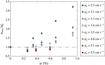
Figure 4 shows the standard deviation of the velocity fluctuations $u_{rms}$ normalised by the incident turbulent fluctuations $u_{0}^{\prime }$ as a function of the gas volume fraction $\unicode[STIX]{x1D6FC}$ for different levels of turbulence. We notice that even after normalisation by the fluctuations of the incident turbulence, the standard deviation of the velocity fluctuations still show a strong dependence both on $\unicode[STIX]{x1D6FC}$ and on $u_{0}^{\prime }$ . In particular, for $u_{0}^{\prime }<3.5~\text{cm}~\text{s}^{-1}$ , the velocity fluctuations are larger than the one produced by the incident turbulence and increase with $\unicode[STIX]{x1D6FC}$ , whereas they are lower for $u_{0}^{\prime }>4.6~\text{cm}~\text{s}^{-1}$ . These two behaviours can be explained by introducing the bubblance parameter $b$ , which compares the energy of the fluctuations produced by the bubble swarm to the one produced by the incident turbulence $u_{0}^{\prime 2}$ . However, predicting theoretically the absolute level of energy produced by a bubble swarm is a difficult task. Following a theoretical approach based on potential theory, it has been shown that this energy is equal to $C_{m}V_{r}^{2}\unicode[STIX]{x1D6FC}$ , where $C_{m}$ is the added mass coefficient (Lance & Bataille Reference Lance and Bataille1991; Van Wijngaarden Reference Van Wijngaarden1998). Experimental work from Riboux et al. (Reference Riboux, Risso and Legendre2010) indicates that the variance of the velocity fluctuations produced by a bubble swarm is equal to $\unicode[STIX]{x1D6FE}^{2}V_{r}^{2}\unicode[STIX]{x1D6FC}$ , where $\unicode[STIX]{x1D6FE}$ is a prefactor which takes into account the anisotropy of the velocity fluctuations in the vertical and horizontal directions ( $\unicode[STIX]{x1D6FE}=1.94$ for the vertical direction). Even if some discussions about the absolute level of the energy produced by a bubble swarm are ongoing, it is reasonable to consider that the energy produced by a bubble swarm is proportional to $V_{r}^{2}\unicode[STIX]{x1D6FC}$ . We thus decided to express the bubblance parameter as

Consequently, $b=0$ corresponds to single-phase flow, whereas $b=\infty$ is for pseudo-turbulence cases. Note that the above definition of the bubblance parameter differs from prior definitions in Rensen et al. (Reference Rensen, Luther and Lohse2005) and Prakash et al. (Reference Prakash, Mercado, van Wijngaarden, Mancilla, Tagawa, Lohse and Sun2016) by the factor $C_{m}=1/2$ . The added mass coefficient $C_{m}=1/2$ comes from potential flow theory for spherical bubbles, while in the present case, we have a swarm of high-Reynolds-number deformable bubbles. Therefore, we chose to define the bubblance parameter without this prefactor (4.1), since this is enough to capture the ratio of the energy of the bubble swarm to that of the incident turbulence. Regardless of the definition chosen, the prefactor does not influence the main conclusions of the present study.

Figure 4.

Standard deviation of the liquid velocity fluctuations in the vertical direction normalised by $u_{0}^{\prime }$ as a function of the gas volume fraction for different levels of turbulence.

Figure 5.

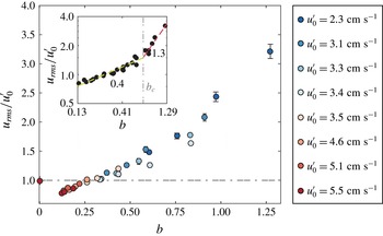
Standard deviation of the liquid velocity fluctuations in the vertical direction normalised by $u_{0}^{\prime }$ as a function of the bubblance parameter. The error bars denote the minimum and maximum values of five equally sampled datasets. Inset shows the same plot on log–log scale.

The strong correlation between the bubblance parameter and the velocity fluctuations is particularly evident from figure 5, in which the standard deviation of the velocity fluctuations $u_{rms}$ normalised by $u_{0}^{\prime }$ is plotted as a function of  $b$ . Regardless of the level of turbulence, all data points collapse on a master curve, which shows a non-monotonic behaviour with the bubblance parameter. For $b<0.27$ , the velocity fluctuations are smaller than the one produced by the incident turbulence. Thus, adding a small amount of bubbles in a very strong incident turbulence deeply modifies the nature of the flow, leading to a reduction in the intensity of the velocity fluctuations, or turbulence attenuation (Mazzitelli, Lohse & Toschi Reference Mazzitelli, Lohse and Toschi2003; Cisse et al. Reference Cisse, Saw, Gibert, Bodenschatz and Bec2015). However, for $b>0.27$ , an enhancement of the velocity fluctuations compared to single-phase flow is observed. Note that the lack of data in the range $0<b<0.13$ limits us from having a complete description of the transition between a single-phase flow and a turbulent bubbly flow evolving at low bubblance parameter. It is, however, difficult to investigate this range of $b$ , since it requires smaller gas volume fractions. The current capillary islands in our water tunnel could not produce a homogeneous bubble swarm at such low gas flow rates.

We will thus now focus only on the turbulent bubbly flows corresponding to $b>0$ . In this regime, the normalised velocity fluctuations increase monotonically with the bubblance parameter. Two regimes can be observed, separated by a critical bubblance parameter $b_{c}\approx 0.7$ (see the inset to figure 5). For $b<b_{c}$ , the normalised velocity fluctuations evolve roughly as $u_{rms}/u_{0}^{\prime }\propto b^{0.4}$ , whereas they increase much faster for $b>b_{c}$ , approximately as $\propto b^{1.3}$ . These two regimes can be related to a stronger contribution of the bubble wakes when the bubblance parameter increases, which will be discussed in § 5.

4.2 Probability density function of the velocity fluctuations

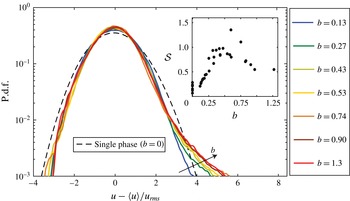
We will now discuss how the structure of the velocity fluctuations depends on the bubblance parameter $b$ . For that purpose, the p.d.f.s of the vertical velocity fluctuations normalised by the standard deviation $u_{rms}$ are plotted in figure 6 for $b$ varied in the range 0–1.3. For $b=0$ , which corresponds to single-phase flow, the p.d.f. of the normalised velocity fluctuations shows nearly Gaussian behaviour. For turbulent bubbly flows ( $b>0$ ), a skewness appears with stronger fluctuations for positive values, but the p.d.f.s remain nearly Gaussian for negative and more probable values. Interestingly, the p.d.f.s do not exhibit exponential tails, as would be expected for pseudo-turbulence ( $b=\infty$ ). It has been shown by Riboux et al. (Reference Riboux, Risso and Legendre2010) that the exponential tails are mainly due to the agitation produced by the wakes in interaction. In a turbulent bubbly flow, the agitation does not result solely from the interactions of the wakes, since the incident turbulence plays a role as well.

Figure 6.

P.d.f. of the liquid velocity fluctuations normalised by $u_{rms}$ for different bubblance parameters. The skewness ${\mathcal{S}}$ of the p.d.f. for increasing $b$ is shown as inset.

The positive skewness of the p.d.f. is also observed experimentally for different operating conditions and is known to be the signature of the bubble wakes (Riboux et al. Reference Riboux, Risso and Legendre2010; Prakash et al. Reference Prakash, Mercado, van Wijngaarden, Mancilla, Tagawa, Lohse and Sun2016). However, in Prakash et al. (Reference Prakash, Mercado, van Wijngaarden, Mancilla, Tagawa, Lohse and Sun2016), they could not observe a clear trend with respect to the $b$ parameter. Here we demonstrate that by increasing the bubblance parameter, the positive skewness increases to a maximum value for $b\approx 0.7$ (inset to figure 6). This can be interpreted as a stronger contribution of the bubble wakes as the bubblance parameter increases. Beyond $b\approx 0.7$ , ${\mathcal{S}}$ appears to decrease a bit before saturating at large values of the bubblance parameter.

4.3 Frequency spectrum of the velocity fluctuations

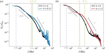
We now investigate the frequency spectrum $S_{zt}$ of the velocity fluctuations for different values of  $b$ . For each operating condition, the spectrum is calculated by averaging at least 180 spectra, each spanning a recording time duration of 8 s, and normalised by $u_{rms}^{2}$ . First, the two-phase flow spectrum is compared to the corresponding single-phase one, for $b=0.13$ (figure 7 a) and $b=1.3$ (figure 7 b). As already seen in § 3.1, the classical $-5/3$ decrease can be observed for single-phase flow in the range of frequency $(1/T_{L};1/\unicode[STIX]{x1D70F}_{\unicode[STIX]{x1D702}})$ . Beyond this range, for $f>1/\unicode[STIX]{x1D70F}_{\unicode[STIX]{x1D702}}$ lies the viscous dissipative range with a very low energy content. The higher negative slope in the dissipative range is expected, and this is likely the range prior to the classical exponential decay (Pope Reference Pope2000).

Figure 7.

Energy spectra of the velocity fluctuations for (a)  $b=0.13$ and (b)  $b=1.3$ . The black curves in (a) and (b) denote the spectrum for the single-phase case before the addition of bubbles.

Figure 8.

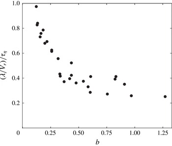
Ratio of the integral time scale ( $\unicode[STIX]{x1D706}/V_{r}$ ) imposed by the bubbles over the dissipative time scale ( $\unicode[STIX]{x1D70F}_{\unicode[STIX]{x1D702}}$ ) in the flow as a function of the bubblance parameter  $b$ .

For the turbulent bubbly flows, the $-5/3$ scaling is still observed for the frequency range $(1/T_{L};1/\unicode[STIX]{x1D70F}_{\unicode[STIX]{x1D702}})$ , and is then followed by $-3$ scaling for higher frequencies. As known from Lance & Bataille (Reference Lance and Bataille1991) and Riboux et al. (Reference Riboux, Risso and Legendre2010), the $-3$ slope is the signature of the bubble-induced turbulence and develops for length scales smaller than $\unicode[STIX]{x1D706}=d/C_{d0}$ , where $C_{d0}$ is the drag coefficient of a single rising bubble. The characteristic time scale $T_{pseudo}$ imposed by the bubble swarm may then be calculated as $T_{pseudo}=\unicode[STIX]{x1D706}/V_{r}$ , and the corresponding frequency scales are shown by the green lines in figure 7(a,b). Irrespective of the bubblance parameter, we observe that the $-3$ scaling subrange starts at the frequency $1/T_{pseudo}=V_{r}/\unicode[STIX]{x1D706}$ . Since the frequency $V_{r}/\unicode[STIX]{x1D706}$ imposed by the bubbles is larger than the Kolmogorov frequency $1/\unicode[STIX]{x1D70F}_{\unicode[STIX]{x1D702}}$ for the range of bubblance parameters studied here (figure 8), we can observe a distinct separation of the time scales in the flow, i.e. the incident turbulence acting for the time scales larger than $\unicode[STIX]{x1D70F}_{\unicode[STIX]{x1D702}}$ , and the bubble-induced turbulence for time scales lower than $\unicode[STIX]{x1D706}/V_{r}$ , which results in two distinct slopes. However, for $b=1.3$ , the spectrum is deformed in the $-5/3$ subrange and presents a bump at $f_{c}\equiv 0.14V_{r}/d\approx 12$  Hz (figure 7 b). Beyond this frequency, we again see the $-3$ slope characteristic of pseudo-turbulence. It may be noted that the steep slope for $f>1/\unicode[STIX]{x1D70F}_{\unicode[STIX]{x1D702}}$ in the single-phase cases is distinctly different from the $-3$ slope of the two-phase cases. This is clear from the fact that the $-3$ slope of two-phase flow has much higher energy content and occurs at larger frequencies as compared to the single-phase cases.

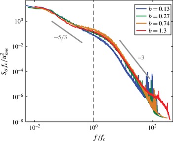
Figure 9 presents the spectrum of the velocity fluctuations normalised by $f_{c}$ for different bubblance parameters. It appears that the bump around $f_{c}$ is present only for $b>0.27$ . This excitation frequency has already been observed by Riboux et al. (Reference Riboux, Legendre and Risso2013) for pseudo-turbulence. The authors attributed it to the injection of energy by the collective wakes instability into the flow. However, this frequency is also comparable to the vortex shedding frequency $f_{v}\equiv St\,V_{r}/d$ of a single bubble at $Re_{b}\approx 500$ , where the Strouhal number $St\approx 0.13$ (Wu & Gharib Reference Wu and Gharib2002; Shew, Poncet & Pinton Reference Shew, Poncet and Pinton2006). It is important to note that this frequency is also close to the one defined by Prakash et al. (Reference Prakash, Mercado, van Wijngaarden, Mancilla, Tagawa, Lohse and Sun2016) as $f_{b}=V_{r}/2\unicode[STIX]{x03C0}d$ . We note that the time-scales separation in the present experiments is too narrow to reveal the true origin of this frequency, but this is an interesting issue for future investigation.

Figure 9.

Energy spectrum of the velocity fluctuations normalised by $f_{c}$ for different values of the bubblance parameter  $b$ .

5.1 Velocity disturbance behind the bubbles

We will now study the velocity disturbance behind individual bubbles. The conditional velocity $u_{c}$ is calculated by averaging the velocity disturbance just behind each detected bubble (at least 1087 bubbles were detected for each measurement point). It is important to mention that the neighbouring bubbles could induce perturbations on the conditional velocity, mainly through their upstream perturbations. The upstream disturbance induced by the next bubble is thus excluded by shortening the detected sample $3(d/V_{b})$ s before the following bubble is detected. The three diameters distance was chosen based on the analysis of Roig & De Tournemine (Reference Roig and De Tournemine2007), where the influence of the upcoming bubble was seen to be minor. We thus checked that in the present study, the upstream perturbation does not exceed three bubble diameters too. 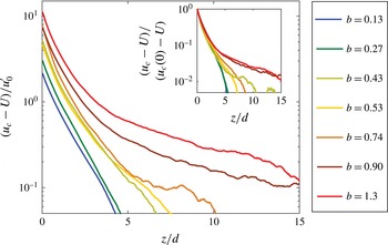Finally, the Taylor hypothesis is used to convert the temporal signal to a spatial one by using the mean rising velocity of the bubbles $V_{b}$ (Hinze Reference Hinze1975). The velocity disturbance behind the bubbles normalised by the turbulent fluctuations $u_{0}^{\prime }$ is shown in figure 10 for different bubblance parameters. It is clear that the bubblance parameter strongly affects the structure of the wake. Both the length of the wake and its shape depend on the bubblance parameter. For low bubblance parameter ( $b<0.7$ ), the wake is around $5d$ long and presents a single exponential decrease. However, when the bubblance parameter is larger than 0.7, the wake length considerably increases, reaching almost $15d$ – $20d$ . Moreover, the conditional mean velocity presents an exponential decrease with a change in slope at a critical distance $z_{c}$ at which $u_{c}(z_{c})-U=u_{0}^{\prime }$ . We can thus distinguish two domains in the wake: a primary wake for $z<z_{c}$ and a secondary wake for $z>z_{c}$ .

Figure 10.

Velocity disturbance behind a bubble in the turbulent bubbly flow. Inset shows the velocity disturbance normalised by $(u_{c}(0)-U)$ , which reveals that the primary wake region is not affected by  $b$ .

Figure 11.

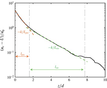
Classification of the bubble-wake into primary wake (PW) and secondary wake (SW) regions. Here $k=1/\ln (10)$ is a prefactor in the slope shown in the above plot.

A primary wake and a secondary wake were also observed by Legendre, Merle & Magnaudet (Reference Legendre, Merle and Magnaudet2006) for a single bubble in a turbulent pipe flow. The primary wake was defined as the region which showed a fast velocity decrease, and the transition from primary wake to secondary wake occurred when the velocity deficit was of the order of the incident turbulence. Following a similar approach, we quantify the primary wake and the secondary wake in our case by defining two characteristic length scales each: a characteristic length $l$ and a characteristic decay length $L$ (figure 11). In the primary wake ( $0<z<l_{pw}$ ), the velocity disturbance is well described by an exponential decrease $u_{c}(z)-U=(u_{c}(0)-U)\times \exp (-z/L_{pw})$ , where $L_{pw}$ is the characteristic decay length of the primary wake. The characteristic length, $l_{pw}$ , is calculated by using the exponential fitting as $u_{c}(z=l_{pw})-U=u_{0}^{\prime }$ . Concerning the secondary wake region, which is defined in the region $l_{pw}<z<l_{sw}$ , the velocity disturbance also follows an exponential decrease, which can be expressed as $u_{c}(z)-U=(u_{c}(l_{pw})-U)\times \exp (-(z-l_{pw})/L_{sw})$ , where $L_{sw}$ is the characteristic decay length of the secondary wake, and $l_{sw}$ is the length of the secondary wake. The length of the secondary wake $l_{sw}$ is defined from the exponential fitting for $u_{c}(z)-U=0.05u_{0}^{\prime }$ . The threshold was chosen as low as possible so that the length of the secondary wake was not underestimated while not taking into account the eventual noise present in the mean velocity deficit far from the bubble interface. In this regard, the value $0.05u_{0}^{\prime }$ seemed to be a reasonable choice. For the fitting of the secondary wake (see figure 11), we checked manually for all the cases that the fits were reasonable. We expect the uncertainties to be within 20 %.

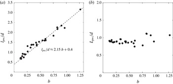
We now focus on the evolution of the characteristic lengths with the bubblance parameter (figures 12 and 13). Concerning the primary wake, the characteristic length $l_{pw}$ increases roughly linearly with $b$ , while the characteristic decay length $L_{pw}$ is almost independent of $b$ (figure 12 a,b). The characteristic length $l_{pw}$ and the decay length $L_{pw}$ are thus controlled by two different mechanisms. The characteristic length of the primary wake is controlled by the ratio between the two sources of turbulence and thus by $b$ . Conversely, since the decay length $L_{pw}$ does not depend on $b$ , this means that the velocity deficit behind a bubble is not affected by the incident turbulence and is only controlled by the perturbation induced by the bubble itself. This is further clarified by the inset to figure 10, which shows that the velocity deficit in the primary wake is not affected by the level of external turbulence. These findings thus extend the observations of Legendre et al. (Reference Legendre, Merle and Magnaudet2006) for a single bubble in turbulence to the case of a dilute bubble swarm. 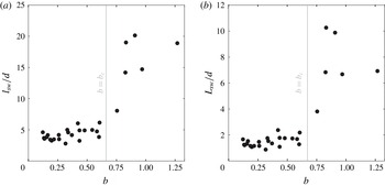Concerning the secondary wake, this presents different characteristics when $b$ increases (figure 13 a,b). In particular, the length of the secondary wake $l_{sw}$ is almost constant for $b<0.7$ , after which it suddenly increases, reaching ${\approx}20d$ for $b>0.8$ . The decay length of the secondary wake $L_{sw}$ presents a similar behaviour. It is constant and close to the decay length of the primary wake for $b<0.7$ , after which it suddenly increases. Consequently, the development of the secondary wake is discontinuous with a threshold at around $b=0.7$ , suggesting that the perturbation induced by the bubble should be strong compared to the external turbulence for the bubbles to develop a large secondary wake. However, the underlying physical mechanisms triggering the secondary wake remain unclear.

Figure 12.

Characteristics of the primary wake. (a) Characteristic length. (b) Characteristic decay length.

Figure 13.

Characteristics of the secondary wake. (a) Characteristic length. (b) Characteristic decay length.

5.2 Conditional p.d.f.

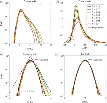
We now carry out a specific study in the vicinity of the bubble. Three regions are distinguished: the primary wake, ( $0<z<l_{pw}$ ), the secondary wake ( $l_{pw}<z<l_{sw}$ ) and the far field ( $l_{sw}<z$ ). Conditional statistical properties of the velocity fluctuations, such as the p.d.f., are calculated in each region by retaining the velocity fluctuations detected in those regions specifically. Figure 14(a,c,d) presents the conditional p.d.f.s normalised by the corresponding standard deviation of the overall velocity fluctuations $u_{rms}$ , for each region and different bubblance parameters. We observe that the shape of the conditional p.d.f.s strongly depends on the region under consideration. In fact, the conditional p.d.f.s of the primary wake are asymmetric, presenting a strong skewness for positive values due to the strong perturbation induced by the bubbles. Remarkably, the p.d.f.s of the velocity fluctuations in the primary wake, once normalised by $V_{r}$ , are similar to the one for a single bubble rising in a quiescent liquid (see figure 14 b and Risso & Ellingsen Reference Risso and Ellingsen2002). This means that the primary wake disturbance arises mainly from the bubble and is not much modified by the external turbulence. In contrast, the conditional p.d.f.s in the far field are Gaussian, meaning that the external turbulence is dominant and that the wake–wake interactions are negligible in this area (figure 14 d). Indeed, it is known from pseudo-turbulence that the exponential tails of the p.d.f. of the velocity fluctuations are the signature of the wake–wake interactions (Risso Reference Risso2016). Concerning the conditioned p.d.f.s of the secondary wake, they are asymmetric, since the tails are exponential for positive fluctuations and Gaussian for negative ones (figure 14 c). In the present case, as the wake–wake interactions are negligible, the secondary wake thus results mainly from the interaction of the wake with the external turbulence, generating the exponential tail of the conditional p.d.f. for the positive fluctuations only. In contrast to wake–wake interaction in pseudo-turbulence, the development of the interactions between the wake and the external turbulence is not an isotropic process in the vertical direction.

Figure 14.

P.d.f.s of the velocity fluctuations for different regions of the wake behind the bubble. (a,b) Primary wake (PW), (c) secondary wake (SW), and (d) far field (FF). The dashed line in (c) represents an exponential distribution of the form $y=\text{e}^{-B\mid u\mid /u_{rms}}$ , where $B=1.25$ , which fits well with the positive fluctuations of the $b=0.13$ case.

Figure 15.

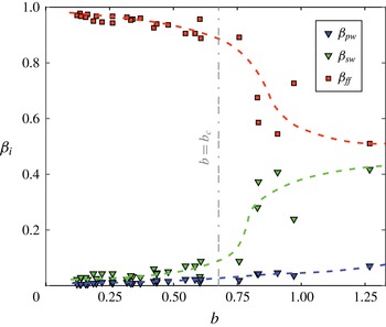
Relative characteristic volume fraction ( $\unicode[STIX]{x1D6FD}$ ) of the primary wake ( $\unicode[STIX]{x1D6FD}_{pw}$ ), secondary wake ( $\unicode[STIX]{x1D6FD}_{sw}$ ) and far field ( $\unicode[STIX]{x1D6FD}_{ff}$ ). The dashed curves in blue, green and red give our interpretation of the evolution of the primary wake, secondary wake and far field, respectively. The fractions sum to 1, i.e. $\unicode[STIX]{x1D6FD}_{pw}+\unicode[STIX]{x1D6FD}_{sw}+\unicode[STIX]{x1D6FD}_{ff}=1$ .

Figure 16.

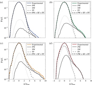
Superposition of the conditional p.d.f.s weighted by their respective volumes for (a)  $b=0.13$ , (b)  $b=0.27$ , (c)  $b=0.74$ and (d)  $b=1.3$ .