1. Introduction
The increase in global energy demand and reliance on fossil fuels has led to significant environmental pollution, impacting air, soil, and water quality (Allen et al. Reference Allen2012). Petroleum hydrocarbons are among the most persistent contaminants due to their chemical stability and slow degradation rates, making them a long-term environmental concern (Overton et al. Reference Overton2022). In aquatic environments, oil pollution originates from sources such as tanker spills, ship operations, and offshore exploration (O’Rourke and Connolly Reference O’Rourke and Connolly2003; Sayed et al. Reference Sayed, Baloo and Sharma2021). Once introduced into the water, petroleum hydrocarbons can alter oxygen levels, contaminate sediments, and disrupt aquatic ecosystems by affecting species behavior, competition, and community structure (Fleeger et al. Reference Fleeger, Carman and Nisbet2003).
In addition to their persistence in water, petroleum hydrocarbons interact with aquatic organisms, particularly algae, which play a central role in aquatic food webs. Over time, as algae grow using nutrients from eutrophic environments, organic contaminants present in water or suspended particles can adsorb onto the surfaces of algae, followed by absorption and biochemical transformation, in addition to photodegradation (Torres et al. Reference Torres2008). This dynamic interaction complicates the distinction between fossil hydrocarbons and biogenic organic matter, particularly because both petroleum, land-derived plant waxes and algae contain n-alkanes of overlapping chain lengths (Meyers and Ishiwatari Reference Meyers and Ishiwatari1993). Biomarker analysis is commonly used to assess petroleum contamination, as hydrocarbons derived from fossil sources carry distinct chemical signatures. However, petroleum hydrocarbons also contain algal-derived biomarkers inherited from their geological formation, making it difficult to differentiate fossil and biogenic sources based only on molecular composition (Killops and Killops Reference Killops and Killops2013).
Radiocarbon dating has been playing a vital role in paleoenvironmental studies in sedimentary marine matrices since the early 1950s (Jones et al. Reference Jones1989; Kershaw Reference Kershaw1986; Taylor Reference Taylor2000). Kershaw (Reference Kershaw1986) discusses the use of radiocarbon dating in deep-sea sediments, which can provide continuous deposition with few hiatuses, allowing scientists to draw conclusions about past climate and carbon cycle changes.
There are important methodological considerations related to radiocarbon measurements in marine samples, particularly the marine reservoir effect, which reflects a systematic offset in
 ${{\rm{\;}}^{14}}$
C between the ocean and the atmosphere. As a result, the
 ${{\rm{\;}}^{14}}$
C content of primary producers in the marine biosphere differs from that of contemporaneous terrestrial primary producers, even at the same point in time (Alves et al. Reference Alves2018; Quarta et al. Reference Quarta2021). However, algae growing at the air–water interface may incorporate dissolved inorganic carbon that is more strongly influenced by atmospheric CO
 ${{\rm{\;}}_2}$
exchange and can therefore display a
 ${{\rm{\;}}^{14}}$
C signature closer to that of the atmosphere. Modern carbon can be present in living algae in a ratio of
 ${{\rm{\;}}^{14}}$
C to total carbon approximately similar to that of atmospheric carbon (Faivre et al. Reference Faivre2015; Scourse et al. Reference Scourse2012; Smith Reference Smith1972; Stenström and Mattsson Reference Stenström and Mattsson2022, Reference Stenström and Mattsson2025; Watanabe and Kuwae Reference Watanabe and Kuwae2015), reflecting the strong coupling between surface waters and the atmosphere, as algae can incorporate atmospheric CO
 ${{\rm{\;}}_2}$
when exposed, implying differences in carbon balance that may indicate a closer linkage to atmospheric carbon.
Radiocarbon is the main method for assessing the percentage of a petroleum-based product (Culp et al. Reference Culp, Cherkinsky and Prasad2014; Norton and Devlin Reference Norton and Devlin2006). In an example of application, measurements of
 ${{\rm{\;}}^{14}}$
C have been utilized to assess the binding of hydrophobic organic contaminants to aquatic sediments through mechanisms such as sorption or chemical binding, providing a quantitative assessment of fossil carbon contributions (Silva et al. Reference Silva2021; White et al. Reference White, Reddy and Eglinton2008) showed an application of the radiocarbon technique by subjecting the collected algae to controlled laboratory conditions, where they produced samples and determined the percentage of modern carbon (pMC) by radiocarbon analysis in SSAMS, a Single Stage Accelerator Mass Spectrometry system, associated with the determination of classical n-alkanes through GC-FID (Gas Chromatography coupled with a Flame Ionization Detector), which brings important fingerprinting of kerosene and diesel in algae.
Crude oil and its products are complex hydrocarbon mixtures ranging from light, short-chain volatile organic compounds to heavy, long-chain, cyclic, branched compounds, and aromatic compounds, with the presence of heteroatoms. The exact composition of petroleum products varies according to the origin of the crude oil and the refining processes (Stout and Wang Reference Stout and Wang2016). The detection of oil contamination in environmental matrices is a field of research with decades of development, and technical notes and protocols containing the fingerprint analysis of crude oil and its products can be found (e.g. Stout and Wang Reference Stout and Wang2016; Wade and Stainken Reference Wade and Stainken2016; Wang et al. Reference Wang2003). Environmental forensic investigations on oil spills have summarized some basic questions on what the product was that was spilled, when did the release occur, and if the spilled product can be related back to the source (Philp Reference Philp2018).
In terms of n-alkane distribution, a typical non-degraded crude oil is dominated by
 ${\rm{n}} - {{\rm{C}}_{1}}$
to
 ${\rm{n}} - {{\rm{C}}_{40}}$
, and as long as the oil gets weathered, the number of heavier alkanes increases in relation to lighter alkanes that are more promptly degraded (Philp Reference Philp2018). Overton et al. (Reference Overton2022) classifies in order of the persistence of compounds when spilled, and the first fraction contains hydrocarbons that can be lost during weathering from minutes to hours (
 ${{\rm n}} - {{{\rm C}}_{1}}$
to
 ${\rm n} - {{\rm C}}_{10}$
, highly-labile fraction), the second from days to weeks (labile
 ${\rm{n}} - {{\rm{C}}_{10}}$
to
 ${{\rm n}} - {{{\rm C}}_{25}}$
fraction), and the third with compounds that slowly degrade from months to years or more (
 ${\rm{n}} - {{\rm{C}}_{25 + }}$
, recalcitrant fraction). Due to this knowledge base, the pronounced odd or even predominance in the n-alkane profile can be related to the source of the material, including plants, algae and bacteria fossilized along the millions of years (Bray and Evans Reference Bray and Evans1961).
The use of some characteristic compounds is another tool for characterization and pattern recognition and process comprehension. A narrow distribution dominated by n-alkane near
 ${\rm{n}} - {{\rm{C}}_{17}}$
may be indicative of oil derived from a marine depositional environment (Philp Reference Philp2018). The presence of the isoprenoids pristane and phytane is commonly related as derived from chlorophyll, and their pristane/phytane ratio is one of the first biomarker parameters proposed to indicate the redox characteristics of the depositional environment of crude oil (Shanmugam Reference Shanmugam1985). Some hydrocarbon regions, such as low chain n-alkanes between
 ${{\rm{C}}_{15}} - {{\rm{C}}_{21}}$
with maxima in
 ${\rm{n}} - {{\rm{C}}_{15}}$
and
 ${\rm{n}} - {{\rm{C}}_{17}}$
are to be derived from algae and bacteria from plankton, and
 ${\rm{n}} - {{\rm{C}}_{23}}$
to
 ${{\rm n}} - {{{\rm C}}_{33}}$
are to be of terrigenous aspect derived from plant waxes with predominance of
 ${\rm{n}} - {{\rm{C}}_{27}}$
,
 ${\rm{n}} - {{\rm{C}}_{29}}$
and
 ${\rm{n}} - {{\rm{C}}_{31}}$
(Volkman et al. Reference Volkman, Revill and Murray1997; Youngblood and Blumer Reference Youngblood and Blumer1973). Carro et al. (Reference Carro, Cobas and Maneiro2006) have shown that n-alkanes with prevalence of
 ${\rm{n}} - {{\rm{C}}_{14}}$
,
 ${\rm{n}} - {{\rm{C}}_{16}}$
,
 ${\rm{n}} - {{\rm{C}}_{18}}$
,
 ${\rm{n}} - {{\rm{C}}_{20}}$
and isoprenoids are due to petrogenic influence.
Based on the literature, the expected results from the proposed techniques include a mixture of fossil-derived organic matter, reflected in an oil-related chemical signature, and the natural background signature of living algae. Although biomarker analysis provides information on hydrocarbon composition, it cannot fully resolve the question of whether the hydrocarbons found in algae are biogenic or derived from fossil contamination. To address this challenge, we applied a dual analytical approach combining radiocarbon analysis and GC-MS-based n-alkane profiling on native algae grown over artificial substrates located in strategic sites to monitor and remove pollutants from water. The radiocarbon analysis assesses the percent Modern Carbon (pMC), reflecting contributions from fossil-derived organic matter and revealing the bulk fossil carbon contamination. Meanwhile, gas chromatography mass spectrometry (GC-MS) analysis of the lipid fraction specifically identifies all n-alkanes, providing molecular-level fingerprinting of algal profile and organic contamination. By combining these complementary methods, we aim to distinguish biogenic from fossil carbon sources, quantify petroleum-derived contamination, and evaluate its implications for aquatic ecosystems.
The application of algae for bioremediation is also favored because while some compounds found in petroleum can be inhibitory to some organisms by reducing the rate of their metabolism or death, some algal species are able to thrive in environments with some rate of pollution. For instance, the growth of U. pertusa algae is supported by lower concentrations of diesel and crude oil, possibly due to the activation of repair mechanisms in response to inappropriate levels of hydrocarbons (Liu et al. Reference Liu2019). However, high concentrations in the water affects algal growth, mainly due to the absorption of hydrocarbons that disrupt photosynthesis and electron transport, and the presence of toxic elements that cause oxidative imbalance, leading to cell damage and inhibited growth (Liu et al. Reference Liu2019). Kalhor et al. (Reference Kalhor2017) reported the total removal of initial oil on water using C. vulgaris in laboratory experiments and showed how different species can behave differently in the presence of oil, with growth of C. vulgaris being enhanced by the increasing of initial oil concentration, while growth of Skeletonema costatum decreased. Microalgae have been reported to be a promising biomonitor for organic and inorganic pollutants (Jay Reference Jay1996; Torres et al. Reference Torres2008), while macroalgae have also been used (DiSalvo et al. Reference DiSalvo, Guard and Try1976; Jacques and McMartin Reference Jacques and McMartin2009; Nayar et al. Reference Nayar, Goh and Chou2005; Nweze and Aniebonam Reference Nweze and Aniebonam2009; Pavoni et al. Reference Pavoni2003; Shaw and Wiggs Reference Shaw and Wiggs1979). Lewis and Pryor (Reference Lewis and Pryor2013) reviews algae used at least once to evaluate the effects of crude, refined and dispersed oils and dispersants showing applicability of Ulva, Caulerpa, Chaetomorpha, and Cladophora green algae species.
The objective of this study is to assess the levels of fossil contamination in algae grown on artificial substrates installed in different locations of a tropical polluted estuary by using
 ${{\rm{\;}}^{14}}$
C-AMS biogenic fraction and determination of n-alkanes. We also evaluate which type of n-alkane profile is related to the % Biogenic Carbon using multivariate analysis. Assessment of risk for oil-contaminated sites can become difficult due to the lack of relevant information on the exposure and toxicity of petroleum mixtures (Heath et al. Reference Heath, Koblis and Sager1993). Therefore, the combination of algae cultivation techniques with the harvesting of native algae from artificial substrates and subsequent analyses, as proposed in this study, can provide a sustainable and low-cost solution to this problem of monitoring pollution. Furthermore, while biomarker analysis provides insight into hydrocarbon composition, it cannot fully resolve the question of whether hydrocarbons found in algae are biogenic or derived from fossil contamination. To address this challenge, we applied a dual analytical approach combining radiocarbon analysis and GC-MS-based n-alkane profiling on wild algae grown over artificial substrates. Ecotoxicological studies in marine biota such as mussels and fishes are well documented (e.g., Baussant et al. Reference Baussant2001; Goldberg Reference Goldberg1975), but algae have a greater potential for biomonitoring oil while continually removing it through their bioremediation mechanisms. In search of effective and economically viable solutions to mitigate the severe effects of pollution, research studies have been showing the potential role that green algae could play in this endeavor (e.g., Hennequin et al. Reference Hennequin2022; Salama et al. Reference Salama2019).
2. Methods
2.1. Study area
The research was carried out in Guanabara bay, located on the southeast coast of Rio de Janeiro, Brazil. This bay has a south-oriented entrance that spans 2 km wide and contains a main channel with depths reaching up to 50 m and extending about 20 km northwards. Despite the presence of this main channel, the overall depth of the bay is relatively shallow (approximately < 10 m) and it primarily experiences influences from saline waters originating from the neighboring South Brazilian continental shelf. These waters are exchanged daily as a result of tidal mixing and freshwater input derived from the smaller surrounding rivers. Located within the inner region of Guanabara Bay, some rivers have been artificially straightened into channels which receive direct inflows containing clandestine domestic and industrial effluents (Kjerfve et al. Reference Kjerfve1997). Moreover, these rivers are also impacted by improper management practices related to water resources in their respective drainage basins. Due to these factors combined over several decades, there has been a substantial degradation in water quality in various areas within Guanabara Bay, as evidenced by studies focused on both its aquatic environments (Brandini et al. Reference Brandini and Rodrigues2016; Cotovicz-Jr. et al. 2015) and sediment analyses (Cordeiro et al. Reference Cordeiro and Machado2015). Low species richness and diversity in marine ecosystems can signal eutrophication, as shown on an ocean submerged rocky substrate near Guanabara Bay (Braga et al. Reference Braga2014).
During periods of the year, especially from September to April, the entrance of colder and more saline nutrient-enriched waters from SACW has been reported inside the bay altering plankton dynamics (Júnior et al. Reference Júnior, Crapez and Barboza2006; Valentin et al. Reference Valentin2021). The exchange of waters is estimated to mix more than half of the waters in the bay in about 12 days (Kjerfve et al. Reference Kjerfve1997), showing the potential of the ecosystem to restore itself despite the well-reported state of pollution. Guanabara Bay provides several ecosystem services that are important for the support of human and well-being, such as artisanal fishing, swimming, sailing, kayaking and other recreational activities. Additionally, many economic activities occur at the bay’s shoreline as with tourism, the ports with goods and cargo transportation and naval maintenance, the petrochemical facilities, and other industries. Semi-sub and drilling ships at the main channel were also part of the bay’s landscapes during periods of the experiment. Traffic of ferryboats is also important for public transportation and can achieve a frequency of up to 20 min at peak rush hour. Shipyards at bay’s waters are also an environmental risk (Aguiar et al. Reference Aguiar, Neto and Fonseca2021).
The geology of Guanabara Bay is primarily composed of igneous and metamorphic rocks, including gneisses and granites, along with recent sediment deposits (Valeriano et al. Reference Valeriano2012). This geological composition suggests a low presence of carbonates, which is an important factor in radiocarbon dating studies. Numerous studies have demonstrated that terrestrial snail shells from the Rio de Janeiro coast serve as a reliable material for both recent and archaeological radiocarbon dating, as their isotopic signatures closely align with expected atmospheric values, indicating a minimal influence from older carbon sources in the region (Carvalho et al. Reference Carvalho2015; Macario et al. Reference Macario2016a). In estuarine environments, the freshwater reservoir effect—caused by carbonate dissolution—must be considered, as it can introduce artificially old radiocarbon ages due to dissolved ancient carbon, a phenomenon observed in certain European rivers (Keaveney and Reimer Reference Keaveny and Reimer2012; Philippsen Reference Philippsen2013). However, in the case of Guanabara Bay, the main rivers feeding the system, such as the Macacu River, originate from non-carbonate terrains (Valeriano et al. Reference Valeriano2012). As a result, there is no significant freshwater reservoir effect that would impact radiocarbon dating in the region.
The marine reservoir effect (MRE) is a well-recognized factor in radiocarbon studies, necessitating the empirical calculation of
 ${\rm{\Delta }}$
R values to correct for deviations in radiocarbon ages (Alves et al. Reference Alves2018). Although
 ${\rm{\Delta }}$
R values for the Rio de Janeiro coast have been progressively refined and are available in the Marine Reservoir Database (http://calib.qub.ac.uk/marine/) (Reimer and Reimer Reference Reimer and Reimer2001), no specific data exist for Guanabara Bay. Furthermore, coastal
 ${\rm{\Delta }}$
R values can exhibit both spatial and temporal variability (Alves et al. Reference Alves2018; Carvalho et al. Reference Carvalho2015; Macario et al. Reference Macario2016a), varying from
 $- 577 \pm 56$
14
C years at ca. 5500 cal BP until
 $- 29 \pm 25$
 ${{\rm{\;}}^{14}}C$
years in the present at a nearby ocean beach (Macario et al. Reference Macario2023). For algal samples that thrive at the water-air interface, it is expected that their primary source of radiocarbon is the atmosphere, meaning the marine reservoir effect is likely to be insignificant in these cases. Although the marine
 ${{\rm{\;}}^{14}}C$
reservoir effect is expected to be minimal for surface-growing algae, we evaluated a conservative worst-case scenario to assess its potential influence on our results. Assuming that up to 25% of the algal carbon derives from marine dissolved inorganic carbon with a
 ${{\rm{\Delta }}^{14}}C$
value of approximately
 $- 45$
‰, and the remaining 75% reflects atmospheric carbon with 0 ‰, the resulting mixed
 ${{\rm{\Delta }}^{14}}C$
value would be around
 $- 11$
‰, by considering
 ${f_{atm}} =$
25% and
 ${f_{marine}} =$
75% on the equation (1) based in Qi and Wang Reference Qi and Wang2019:
 ${{\rm{\Delta }}^{14}}{C_{mix}} = {f_{atm}} \cdot {{\rm{\Delta }}^{14}}{C_{atm}} + {f_{marine}} \cdot {{\rm{\Delta }}^{14}}{C_{marine}}$
This shift is small relative to the
 ${{\rm{\Delta }}^{14}}C$
signature of fossil carbon
 $\approx - 1000$
‰ (Qi and Wang Reference Qi and Wang2019), and would not significantly affect the estimated fossil carbon contributions or the interpretation of spatial pollution patterns. The value of
 ${{\rm{\Delta }}^{14}}{C_{marine}} \approx -45$
‰ is obtained by converting an approximate local reservoir age of 371 years, calculated as (400-29), using the relationship
 $\Delta^{14}C = 1000\left(e^{-371/8033}-1\right).$
Therefore, even under this conservative scenario, the influence of the marine reservoir effect on our conclusions is negligible.
2.2. Sampling strategy
Three sampling sites located at Guanabara Bay were strategically selected for our in situ experiment, near a ferry station (–22.93239ºS, –43.11109ºW, referred to as BAR), on an estuarine recreational beach (–22.90981ºS, –43.12982ºW, near Boa Viagem, referred to as BV), and inside a mussel farm (–22.93239ºS, –43.11109ºW, referred to as MAR from mariculture) (Figure 1). It is hypothesized that the referred sequence could represent a decreasing gradient of pollution due to a higher vessel traffic in the ferry station, later on Boa Viagem due to drilling ships nearby and closer distance from the bay’s entrance, then in the mariculture farm which has the influence of filter-feeding organisms.
Partially showing the city of Rio de Janeiro to the west, with Guanabara Bay in the center and Niterói city to the east. The numbers 1, 2 and 3 refer to the sampling sites (BAR, BV, and MAR, respectively).

During the period of the experiment we monitored the floating structures on a daily basis to follow algal growth over the screen allowing for an estimate of ideal algal biomass over the area, which was enough for the chemical analyses. The artificial substrates were started on 15/Dec/2021 at BV station, 21/Dec/2021 at MAR station, 22/Dec/2021 at BAR station.
The area for colonization of the algal community consisted mainly of a HDPE screen that works as a substrate with 1 m
 ${{\rm{\;}}^2}$
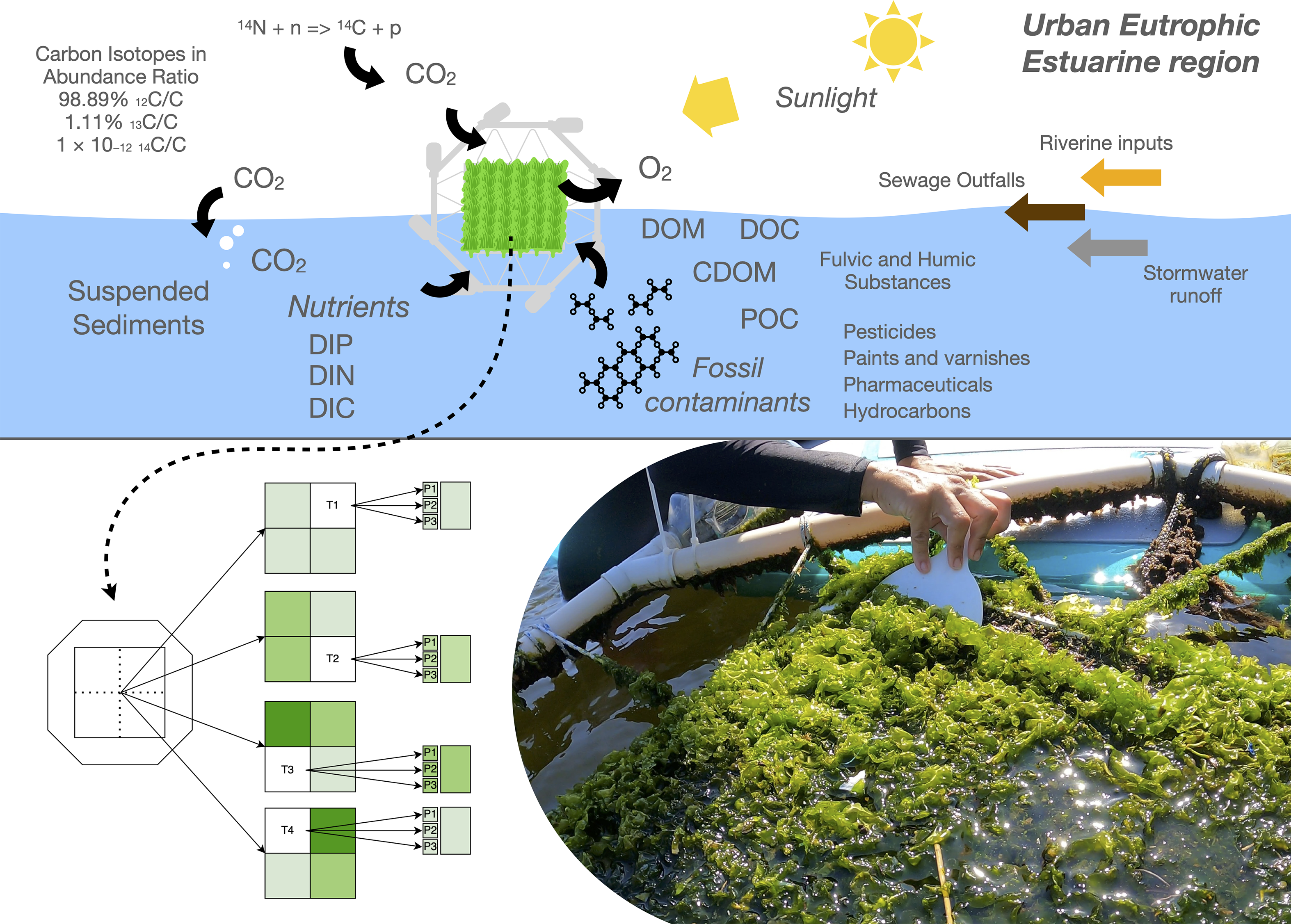
of area (Figure 2) that was fixed to floating structures made with PVC pipes, connections and recycled PET bottles. The floating structure was anchored to the monitoring sites, presenting a free-motion movement around a radius of actuation.
A conceptual model designed and applied for the identification of fossil contamination in native algae using radiocarbon and n-alkanes determination, sampling strategy and experimental setup.

We collected samples periodically within 2 to 5 weeks of exposure in the environment by collecting algae from a random location on the screens. The samples are collected by scrubbing the screen, while approximately 99% of the substrate is cleaned. A small portion of native fragments and biofilm is intentionally left behind to serve as an inoculum for the next algal community to establish and grow, as occurs in other artificial substrates (Adey et al. Reference Adey2013; Liu et al. Reference Liu2017).
Random replicates of a quadrant of the 1 m
 ${{\rm{\;}}^2}$
screen were obtained in different stages of growth at the Sampling Times
 ${{\rm{T}}_1}$
,
 ${{\rm{T}}_2}$
,
 ${{\rm{T}}_3}$
, and
 ${{\rm{T}}_4}$
, which were approximately 2, 2–3, 3–4 and 4–5 weeks of duration, respectively (Figure 2). The replicas were sorted with random numbers from 1 to 9, corresponding to screens locations, and collected separately by scrapping algal biomass from the screens using a spatula. The excess water from the biomass was gently removed with a 2 mm sieve and stored in identified zip-loc bags that were placed inside a styrofoam box in the dark until the lab. Three replicates (
 ${{\rm{P}}_1}$
,
 ${{\rm{P}}_2}$
,
 ${{\rm{P}}_3}$
) were demarcated, scraped, placed individually in ziploc bags, and stored. Biomass samples remained stored < 4 ºC until sorting was done in less than 24 hr.
2.3. Algal analyses
The algae used in this study were manually cleaned to remove macroscopic organic debris, benthic invertebrates, and other undesired visible non-algal material with the aid of lab inox tweezers and stored in acid-washed pre-weighted glass recipients. The recipients were taken to a lyophilizer for 24–48 hr, where water was removed. Aliquots of the randomly dried algae were then weighted with the necessary amount for the analyses, i.e., 0.5–2 g for n-alkanes,
 $\approx$
7 mg for
 ${{\rm{\;}}^{14}}$
C biogenic/fossil fraction on SSAMS. Dried samples were subjected to the same extraction and fractionation method of (Silva et al. Reference Silva2021) for the determination of n-alkane concentrations. As a modification, dried algal biomass was grinded to enhance surface area during extraction and sieved by a 1 mm mesh to avoid any external contamination of non-algal particles. For extraction, 6 mL of dichloromethane were added to the vials containing between 0.5–2.5 g of dried algae, mixed in the vortex for 60 s, taken to the ultrasonic bath for 15 min, centrifuged for 5 min, and the supernatant was transferred to a round-bottom balloon with a calcinated pasteur pipette. This procedure was repeated with dichloromethane, and then with a dichloromethane:methanol (50:50) solution. The total lipid extract (TLE) was eluted with 2 mL of hexane, spiked with 50
 $\mu$
L of recovery standard, and taken to a silica chromatographic column to obtain alkane fraction eluting with 2 mL of hexane and collecting in 4 mL vials. Fractionated extracts were then dried in a nitrogen purge and kept frozen until analysis. Redissolution of the concentrated extract was done minutes before injection in the GC-FID with 100
 $\mu$
L of hexane containing the internal standard
 ${\rm{n}} - {{\rm{C}}_{30}} + {{\rm{D}}_{62}}$
at 20
 $\mu$
g.L
 ${{\rm{\;}}^{ - 1}}$
. Finally, the concentrated liquid was separated by Agilent 6890 GC-FID and analyzed quantitatively by the internal standard method. The column was a DB-5 flexible quartz capillary (30 m × 0.25 mm, df 0.25
 $\mu$
m). The oven was held at 50 ºC for 1 min, heated to 320
 ${{\rm{\;}}^o}$
C at a rate of 6 °C.min
 ${{\rm{\;}}^{ - 1}}$
, held for 10 min. Hydrogen was used as carried gas, and the flow rate was maintained constant at 7.9 mL.min
 ${{\rm{\;}}^{ - 1}}$
. The flux at the injector was 21.0 mL.L
 ${{\rm{\;}}^{ - 1}}$
for a split ratio of 10:1 and a temperature at 280 ºC. Limit of detection (LOD) was calculated as LOD = (3.3 Std. Dev. df)/ slope of the line, where Std. Dev. is the standard deviation of the analytic signal ratio by the internal standard signal of 10 blank solutions, and df is the sample dilution factor. Concentration of n-alkanes
 ${{\rm{C}}_8} - {{\rm{C}}_{40}}$
and isoprenoids pristane and phytane were determined and calculated based on the area of the integrated chromatographic peaks normalized by the area of the internal standard for each compound.
All samples were freeze-dried (Freeze-dryer Alpha model 1-2 LD plus, Martin Christ) and placed inside prebaked quartz tubes containing silver powder and cupric oxide. They were then combusted at 900 ºC for 3 hr in a muffle oven. The resulting gas was purified using dry ice/ethanol traps within a stainless-steel graphitization line (Macario et al. Reference Macario2013). Graphitization was performed using the zinc/titanium hydride method with an iron catalyst (Xu et al. Reference Xu2007). The sealed tubes were heated in a muffle oven (Jung Ltda.) at 550 °C for 7 hr. The graphitized samples were then pressed into individual cathodes, mounted on the cathode wheel of the ion source, and measured using the 250 kV SSAMS system, assembled by NEC (National Electrostatics Corp.) at the Radiocarbon Laboratory, Physics Institute. Isotopic fractionation was corrected by online
 ${{\rm{\;}}^{13}}C$
measurement in the accelerator. Background levels were assessed using processed graphite samples, yielding an average
 ${{\rm{\;}}^{14}}{\rm{C}}{/^{13}}{\rm{C}}$
ratio of
 $6 \times {10^{ - 13}}$
, while the unprocessed graphite showed a machine background of
 ${10^{ - 13}}$
. Accuracy was verified by analyzing reference materials, with mean results close to the expected values: Oxalic Acid II 134.04
 $\pm$
0.26 pMC, C6-IAEA (sucrose) 150.19
 $\pm$
0.42 pMC, and Reactor Graphite 0.52
 $\pm$
0.01 pMC. Following the laboratory standards for the determination of the Biogenic Fraction in biobased material (Silva et al. Reference Silva2021; Santos et al. Reference Santos2019; Jou et al. Reference Jou2021), the biogenic fraction was then obtained using the procedure described by (Norton and Devlin Reference Norton and Devlin2006) by the application of the norm ASTM D6866 (as discussed in the Standard Test Methods for Determining the Biobased Content of Solid, Liquid, and Gaseous Samples Using Radiocarbon Analysis 2021) (ASTM 2021). The fossil carbon content is calculated based on the biogenic carbon %. Considering the algae grown under the same atmospheric conditions, all samples were treated uniformly in accordance with ASTM D6866:2021, using a normalization factor of 1.0. A 100% biogenic sample is in equilibrium with the atmosphere. pMC values below 100 were directly converted to biogenic content, whereas pMC values exceeding 100, resulted in calculated biogenic fractions greater than 1 and were therefore reported as 100%, in accordance with the limit established by the standard. The method is based on controlled studies that identified an inter-laboratory total uncertainty up to
 $\pm 3$
% to be considered the uncertainty of the biogenic fraction.
3. Results and discussions
A total of 10 algal samples collected from the artificial substrates were analyzed, with growth periods ranging from 2 to 5 weeks (Table 1). Total n-alkane concentrations found in algae grown on floating artificial substrates ranged from 1.45 to 125.38
 $\mu$
g.g
 ${{\rm{\;}}^{ - 1}}$
DW, with a median of 6.95
 $\mu$
g.g
 ${{\rm{\;}}^{ - 1}}$
DW and an average of 21.18
 $\mu$
g.g
 ${{\rm{\;}}^{ - 1}}$
DW (N = 10). Algal biogenic fraction varied from 51 to 100%, with the highest fossil content and total n-alkane concentration observed at the ferry station (BAR T2, 23 days of growth, collected from Jan–Feb/2022). In this sample,
 ${\rm{n}} - {{\rm{C}}_{27}}$
was the dominant alkane (18.90
 $\mu$
g.g
 ${{\rm{\;}}^{ - 1}}$
DW, 15% of total n-alkanes). For comparison, Silva et al. (Reference Silva2021) reported a maximum n-alkane concentration of 15.61
 $\mu$
g.g
 ${{\rm{\;}}^{ - 1}}$
in the algae mixed with diesel, while control algae from the same estuarine beach contained only 0.01
 $\mu$
g.g
 ${{\rm{\;}}^{ - 1}}$
. The concentrations found in this study are therefore high when compared to previous reports.
Summary of algal growth conditions, sampling, radiocarbon content (pMC), biogenic fraction (%), and total n-alkane concentrations.

Table 1 Long description
The table contains 10 rows and 8 columns. Column headers are Lab I D, Sampling period, Station, Sampling time, Growth days, Percent Modern Carbon pMC, Biogenic fraction (%), and Total n-alkanes (μg g⁻¹). Row 1: Lab I D, 220140; Sampling period, Dec-Jan; Station, BAR; Sampling time, T3; Growth days, 29; Percent Modern Carbon pMC, 80.72 ± 0.58; Biogenic fraction (%), 81; Total n-alkanes (μg g⁻¹), 5.46. Row 2: Lab I D, 220115; Sampling period, Dec-Jan; Station, BV; Sampling time, T4; Growth days, 35; Percent Modern Carbon pMC, 102.55 ± 0.64; Biogenic fraction (%), 100; Total n-alkanes (μg g⁻¹), 5.44. Row 3: Lab I D, 220116; Sampling period, Dec-Jan; Station, MAR; Sampling time, T3; Growth days, 28; Percent Modern Carbon pMC, 96.74 ± 0.69; Biogenic fraction (%), 97; Total n-alkanes (μg g⁻¹), 1.45. Row 4: Lab I D, 220143; Sampling period, Jan-Feb; Station, BAR; Sampling time, T1; Growth days, 15; Percent Modern Carbon pMC, 99.32 ± 0.67; Biogenic fraction (%), 99; Total n-alkanes (μg g⁻¹), 7.51. Row 5: Lab I D, 220118; Sampling period, Jan-Feb; Station, BAR; Sampling time, T2; Growth days, 23; Percent Modern Carbon pMC, 50.50 ± 0.35; Biogenic fraction (%), 51; Total n-alkanes (μg g⁻¹), 125.38. Row 6: Lab I D, 220141; Sampling period, Jan-Feb; Station, BV; Sampling time, T1; Growth days, 15; Percent Modern Carbon pMC, 96.87 ± 1.00; Biogenic fraction (%), 97; Total n-alkanes (μg g⁻¹), 5.26. Row 7: Lab I D, 220142; Sampling period, Jan-Feb; Station, MAR; Sampling time, T1; Growth days, 15; Percent Modern Carbon pMC, 91.28 ± 0.91; Biogenic fraction (%), 91; Total n-alkanes (μg g⁻¹), 6.40. Row 8: Lab I D, 220117; Sampling period, Jan-Feb; Station, MAR; Sampling time, T2; Growth days, 23; Percent Modern Carbon pMC, 101.73 ± 0.56; Biogenic fraction (%), 100; Total n-alkanes (μg g⁻¹), 35.68. Row 9: Lab I D, 220319; Sampling period, Feb-Mar; Station, BV; Sampling time, T1; Growth days, 14; Percent Modern Carbon pMC, 85.75 ± 0.86; Biogenic fraction (%), 86; Total n-alkanes (μg g⁻¹), 9.21. Row 10: Lab I D, 220337; Sampling period, Feb-Mar; Station, MAR; Sampling time, T1; Growth days, 14; Percent Modern Carbon pMC, 103.13 ± 0.31; Biogenic fraction (%), 100; Total n-alkanes (μg g⁻¹), 10.02.
 ${{\rm{\;}}^{\rm{*}}}$
Biogenic fraction uncertainty was fixed at 3% following the ASTM D6866:2021 standard.
When comparing the first contemporary algae sampled 4–5 weeks after implementation from Dec/2021 to Jan/2022, radiocarbon analysis exhibited biogenic fraction ranging from 81% at the ferry station (BAR T3) to 100% at the estuarine beach (BV T4) (Table 1, Figure 3, while in the mariculture site (MAR T3) contained 97% of biogenic fraction. Despite the low fossil content in the estuarine beach sample, n-heptacosane (
 ${\rm{n}} - {{\rm{C}}_{27}}$
) was the most abundant n-alkane. While
 ${\rm{n}} - {{\rm{C}}_{27}}$
occurs naturally in algae (Binark et al. Reference Binark2000), its presence can also indicate fossil hydrocarbon influence. For instance, Silva et al. (Reference Silva2021) detected
 ${\rm{n}} - {{\rm{C}}_{27}}$
as the most concentrated alkane (150.3 ng.g
 ${{\rm{\;}}^{ - 1}}$
) in algae exposed to 15 mL of kerosene, demonstrating its potential as an indicator of petroleum contamination.
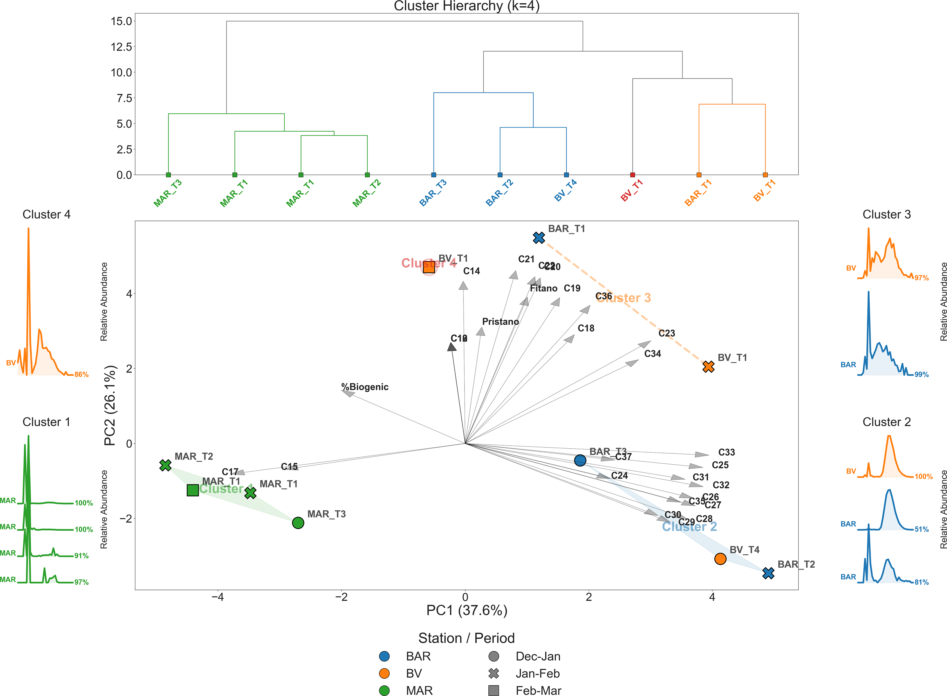
Integrated hierarchical clustering, principal component analysis (PCA), and n-alkane profile characterization of algal samples grown on artificial substrates. The upper panel shows hierarchical clustering (Ward’s method, k = 4) based on standardized relative n-alkane abundances, revealing four chemically distinct clusters. The central panel presents a PCA biplot (PC1 = 37.6%, PC2 = 26.1%) with vectors representing individual n-alkanes and the biogenic fraction. Samples are colored by cluster, with symbols indicating station (BAR, BV, MAR) and sampling period. Convex hulls and dashed connectors highlight cluster structure in ordination space. Side panels display stacked relative n-alkane profiles for each cluster, annotated with the corresponding radiocarbon-derived biogenic fraction percentages.

Algae collected at consecutive sampling times in the period from Jan/2022 to Feb/2022 showed an increase in fossil carbon at the ferry station (BAR T1 and BAR T2) from 99% to 51% of biogenic fraction, indicating ongoing fossil contamination and hydrocarbon accumulation by algae. In contrast, no such trend was observed at the mariculture station in the same sampling period, where fossil carbon levels decreased (MAR T1 to MAR T2: from 91% to 100% of biogenic fraction). This decline suggests either an absence of new petroleum inputs at the site during the second sampling and/or a potential depuration of fossil hydrocarbons through biodegradation from algal tissue over time; the same was observed in the third sampling of MAR station. In the third sampling, algae from the estuarine beach showed the lowest biogenic fraction from all samplings in this station (86%).
Among the locations, samples from the ferry station (BAR) exhibited the highest mean total n-alkanes and lowest biogenic fraction compared to the estuarine beach (BV) and the mussel farm in Jurujuba sound (MAR), although the differences were not statistically significant (p > 0.05). The restricted circulation near the mariculture site and the greater exposure to vessel traffic at the ferry station may further contribute to pollutant accumulation. The dominant species identified belonged to the Ulva and Enteromorpha, which are common green algae in aquatic environments (Nassar Reference Nassar2012). The most abundant n-alkanes detected were as
 ${\rm{n}} - {{\rm{C}}_{17}}$
(70%), then
 ${\rm{n}} - {{\rm{C}}_{27}}$
(20%), and
 ${\rm{n}} - {{\rm{C}}_{15}}$
(10%) (Table 1), indicating a mixed contribution of biogenic and potential fossil-derived hydrocarbons.
Early-stage samples (<15 days of growth) already exhibited high but variable biogenic fractions (86–100%), despite relatively low total n-alkane concentrations (mean = 7.68
 $\mu$
g.g
 ${{\rm{\;}}^{ - 1}}$
DW). This indicates that detectable fossil carbon can be present within the first two weeks of algal development, even when molecular profiles are dominated by algal-derived hydrocarbons. Samples grown for longer periods (>15 days) also showed variable (51–100%) biogenic fraction and substantially higher variability in total n-alkane concentrations (mean = 34.68
 $\mu$
g.g
 ${{\rm{\;}}^{ - 1}}$
DW; median = 5.45
 $\mu$
g.g
 ${{\rm{\;}}^{ - 1}}$
DW), indicating that the variability of fossil contamination can be detected and monitored from early-stage to longer periods of exposition.
Notably, the sample with the highest total n-alkane concentration (125.38
 $\mu$
g.g
 ${{\rm{\;}}^{ - 1}}$
DW) also exhibited the lowest biogenic fraction (51% biogenic fraction), while other long-growth samples with very low alkane concentrations retained an almost exclusively biogenic radiocarbon signature. From the highest measured radiocarbon content (100% biogenic fraction) samples found in the sample mariculture station (MAR T2, Jan–Feb) presented
 ${\rm{n}} - {{\rm{C}}_{15}}$
accounting for half of the total n-alkanes. In contrast, a sample near the ferry station (BAR T2, Jan–Feb) showed 51% of biogenic fraction with
 ${\rm{n}} - {{\rm{C}}_{27}}$
accounting to 15% of Total n-alkanes. This sample also had the highest n-alkanes concentration, more than three times that of the second most concentrated sample, which originated from a mariculture station and was dominated by
 ${\rm{n}} - {{\rm{C}}_{17}}$
(67.2% from Total n-alkanes).
Despite the high concentration of total n-alkanes in the mariculture sample, radiocarbon analysis showed only trace fossil contamination, suggesting a predominantly biogenic source of hydrocarbons in that environment. Following the literature, studies have shown that n-pentadecane (
 ${\rm{n}} - {{\rm{C}}_{15}}$
) was the most characteristic alkane in Ulva and Enteromorpha spp. The hydrocarbons of Enteromorpha intestinalis grown in clean water are represented by n-alkanes
 ${\rm{n}} - {{\rm{C}}_{17}}$
and
 ${\rm{n}} - {{\rm{C}}_{19}}$
, while polluted samples of the same species contain a wider range from
 ${\rm{n}} - {{\rm{C}}_{14}}$
to
 ${\rm{n}} - {{\rm{C}}_{24}}$
(Mironov et al. Reference Mironov, Shchekaturina and Tsimbal1981). Ulva rigida presented unbranched alkanes from
 ${\rm{n}} - {{\rm{C}}_{14}}$
to
 ${\rm{n}} - {{\rm{C}}_{22}}$
with a predominance of
 ${\rm{n}} - {{\rm{C}}_{17}}$
, while the thalli of polluted areas contained
 ${\rm{n}} - {{\rm{C}}_{11}}$
to
 ${\rm{n}} - {{\rm{C}}_{13}}$
, as well as the isoprenoids Pristane and Phytane. Thus, samples from the same algal species taken from different areas showed significant divergences on the chromatograms (Mironov et al. Reference Mironov1981), but a predominance of
 ${\rm{n}} - {{\rm{C}}_{15}}$
,
 ${\rm{n}} - {{\rm{C}}_{17}}$
is expected for algae (Programme Reference Programme1992).
Fossil carbon incorporation is not solely driven by alkane’s fraction, but enters the algal biomass through multiple pathways, including adsorption of dissolved organic carbon, association with fine particulate matter, and retention within the growing biofilm matrix (Figure 2). As algal thalli develop live exposed in the water column, they act as integrative surfaces which are capable of bioaccumulating pollutant signals beyond their internally produced hydrocarbons. Importantly, the presence of fossil carbon in samples collected in all sampling times suggests that algae can record ambient hydrocarbon contamination shortly after deployment, while prolonged exposure increases the probability of integrating other specific contamination events and biotransformation of molecules, rather than producing a monotonic growth-related trend. These results highlight that radiocarbon signatures in algal biomass reinforces the value of algae as sensitive, time-integrated monitors of fossil carbon inputs in aquatic systems.
The fossil loading in these samples may also be influenced by other substances not captured in this integrated analysis, such as aromatic hydrocarbons (PAHs), polychlorinated biphenyls (PCBs), organochlorine pesticides, plastic-derived contaminants including phthalates, bisphenols, and other emerging pollutants including per- and polyfluoroalkyl substances (PFAS), flame retardants (PBDEs), and pharmaceutical and personal care products (PPCPs). Consequently, the observed variation in biogenic fraction cannot be attributed solely to n-alkane concentrations. Further analysis involving a broader suite of organic biomarkers and contaminants of emerging concern (CECs) is required to provide a comprehensive landscape of the fossil contaminants present and to determine if a true threshold effect exists at higher loading levels.
As Binark et al. (Reference Binark2000) discussed, the dominant alkane composition in algae is highly dependent on environmental conditions and the location of collection. Some authors have shown that hydrocarbons can be assimilated by algae in a short period of time (El-Shoubaky and Mohammad Reference El-Shoubaky and Mohammad2016; Silva et al. Reference Silva2021). A study has shown that after 24 hours, gasoline is already absorbed by Ulva and Enteromorpha species (El-Shoubaky and Mohammad Reference El-Shoubaky and Mohammad2016). Silva et al. (Reference Silva2021) demonstrated in a laboratory experiment that Ulva can accumulate hydrocarbons from diesel fuel and kerosene in one hour. When oil is in the water, it may become externally adhered and undergo a degradation process initiated by the microecosystem at the surface of the algae. In addition, organic pollutants can be stored in the tissues of algae, with uptake varying depending on the specific species (Torres et al. Reference Torres2008). An expansion of algal growth could potentially dilute fossil content through tissue growth, a phenomenon that represents an increase in biogenic fraction beyond concurrent biodegradation processes. The ability of algae to rapidly accumulate hydrocarbons from diesel and kerosene can be beneficial for environmental cleanup efforts, as it can provide valuable indicators for assessing the impact of contaminants in coastal areas, thus aiding in the understanding of pollution mechanisms and potential sources. Additionally, the strategy of collecting algae from the artificial substrates also provides eutrophication and fossil contamination mitigation.
Multivariate statistics such as principal component analysis (PCA) have been used for pattern recognition of chemical data (Petrisor Reference Petrisor2014). PCA of the scaled variables (n-alkanes and fossil fraction) was performed to extract significant PC’s and to further reduce the contribution of variables with minor significance, as follows (Krishna et al. Reference Krishna, Satyanarayanan and Govil2009). The Figure 3 shows the distribution of principal components, with samples clustered by Ward’s distance in the n-alkanes distribution dataset, along with biogenic fraction through radiocarbon analysis. The multivariate analysis reveals four chemically and environmentally distinct clusters, consistently resolved across the PCA ordination, hierarchical clustering, and stacked alkane profiles (Figure 3).
Cluster 1, composed exclusively of samples from the MAR site, is characterized by a pronounced enrichment in mid-chain n-alkanes relative to all other samples. This molecular signature is accompanied by the highest biogenic contribution, which is clearly visible in the stacked profiles. In the PCA, it is reflected by the cluster’s strong association with the negative side of PC1, indicating a dominant influence of fresh, autochthonous organic matter. Cluster 2 comprises samples from BAR T3 and BV T4, collected during the Dec–Jan period, highlighting a strong temporal influence on molecular composition. These samples exhibit a homogeneous, bell-like alkane distribution dominated by long-chain compounds, indicative of more uniform inputs, possibly from petrogenic or reworked organic matter, as seen from the biogenic fraction vector as in the PCA, they separate clearly from Cluster 1 along PC1, positioned on the opposite side of the axis and showing lower relative biogenic percentages.
Meanwhile, Cluster 3 exhibits a different pattern: a chain-like distribution skewed toward higher carbon numbers, reflecting progressive enrichment in long-chain n-alkanes without a dominant single homologue. In the PCA, these samples plot in the upper positive region of PC2, indicating that this axis captures variations in chain-length organization and molecular continuity rather than total biogenic contribution. Cluster 4 exhibits a broadly similar long-chain structure to Cluster 3 but differs by a higher contribution of C17, along with detectable inputs from lighter hydrocarbons. This mixed signature suggests a superposition of fresh algal production mixed with a background of longer-chain material. In the PCA, Cluster 4 also occupies the positive PC2 domain but separates from Cluster 3 due to, apparently, its stronger association with mid-chain compounds.
The relative concentration of the n-alkanes homologues from
 ${\rm{n}} - {{\rm{C}}_{10}}$
to
 ${\rm{n}} - {{\rm{C}}_{40}}$
across different sampling sites and algal growth stages is shown in Figure 3. The presence of petroleum-derived hydrocarbons is indicated by the lack of a clear preference for even or odd n-alkanes, a characteristic feature of petrogenic contamination. Most samples exhibited a bimodal distribution of n-alkanes, with concentration peaks around
 ${\rm{n}} - {{\rm{C}}_{17}}$
and
 ${\rm{n}} - {{\rm{C}}_{27}}$
(Figure 3). These peaks did not occur in isolation but were accompanied by neighboring homologues, forming a uniform distribution rather than the chain-like pattern with odd preference typical of terrigenous sources, which further supports the greater influence of fossil hydrocarbons. Peak concentrations were most commonly observed near
 ${\rm{n}} - {{\rm{C}}_{15}}$
and
 ${\rm{n}} - {{\rm{C}}_{17}}$
, compounds frequently associated with algae (Shaw and Wiggs Reference Shaw and Wiggs1979), while near
 ${\rm{n}} - {{\rm{C}}_{27}}$
reflects a combination of terrestrial plant waxes, anthropogenic inputs, and algal contributions. Additional inputs from epiphytic diatoms, which also produce n-alkanes, may contribute to the overall profile, but to a lesser extent.
By integrating the principal component analysis, the hierarchical clustering, and the stacked profiles in a single picture reveals that PC1 primarily tracks a gradient in biogenic contribution, whereas PC2 highlights differences in the relative dominance of mid- versus long-chain compounds. The extent of fossil hydrocarbon contamination in water evaporation can be influenced by many factors. Compounds with lower carbon numbers show greater water solubility compared to those with higher carbon numbers, although overall solubility is minimal. Under typical conditions, it is expected that hydrocarbons up to approximately
 ${{\rm{C}}_{12}} - {{\rm{C}}_{15}}$
can evaporate (Stout and Wang Reference Stout and Wang2016). In addition to dissolution and evaporation other factors can significantly influence hydrocarbon pollution in the water. These include adsorption, where pollutants adhere to the surface of materials like suspended sediments, reducing their availability in the water column. Algae and bacteria that live in the water and in the artificial substrates are the other expected surfaces where contaminants can adhere. Temperature and salinity also have a role, as they can affect the speed of biodegradation processes and the solubility of hydrocarbons (Stout and Wang Reference Stout and Wang2016). The availability of oxygen and nutrients is necessary for bacterial growth, promoting the natural degradation of hydrocarbons. The level of water turbulence also matters as it affects the distribution and dilution of hydrocarbons. Sunlight can also break down certain types of hydrocarbons (Stout and Wang Reference Stout and Wang2016). Furthermore, the type of hydrocarbons and the specific composition of the oil spill can influence the rate of degradation and the overall environmental impact.
As a comparison of reported hydrocarbons in algae, Shaw and Wiggs (Reference Shaw and Wiggs1979) showed that Enteromorpha linza collected in a large tidal estuary in south-central Alaska were dominated by
 ${\rm{n}} - {{\rm{C}}_{15}}$
as the most abundant of the saturated ones (8% of Total hydrocarbons) with
 ${\rm{n}} - {{\rm{C}}_{17}}$
and
 ${\rm{n}} - {{\rm{C}}_{15}}$
as the most abundant hydrocarbons from the algal species analyzed. Yang et al. (Reference Yang2018) showed a summary with Total n-alkanes in representative environmental samples with
 ${\rm{n}} - {{\rm{C}}_{17}}$
as a common alkane reported in algae. Major n-alkane found on a sample of mixed zoo- and phytoplankton from Tarpaulin Cove in Massachusetts was
 ${\rm{n}} - {{\rm{C}}_{17}}$
, and lower concentrations of other
 ${\rm{n}} - {{\rm{C}}_{14}}$
to
 ${\rm{n}} - {{\rm{C}}_{29}}$
n-alkanes were found (Clark Reference Clark1966). The presence of large amounts of
 ${\rm{n}} - {{\rm{C}}_{18}}$
to
 ${\rm{n}} - {{\rm{C}}_{37}}$
alkanes in some samples was believed to be good evidence for petroleum contamination (Middleditch et al. Reference Middleditch, Chang and Basile1979). According with a study in the Qinghai-Tibetan Plateau, the concentrations of hydrocarbons in Cladophora and Spirogyra were found relatively low, ranging on average from 2-4
 $\mu$
g.g
 ${{\rm{\;}}^{ - 1}}$
DW, respectively (max. 5.9 and 8.6
 $\mu$
g.g
 ${{\rm{\;}}^{ - 1}}$
DW); compound maxima in both algae was at
 ${\rm{n}} - {{\rm{C}}_{27}}$
and profile showed a relatively high long chain (
 ${{\rm{C}}_{27}} - {{\rm{C}}_{33}}$
) abundance (Liu and Liu Reference Liu and Liu2016).
The algae in our research had a Total n-alkanes concentration higher than from the Chinese coastal sediments from Pearl River Estuary (0.53 – 0.87
 $\mu$
g.g
 ${{\rm{\;}}^{ - 1}}$
DW), Yellow River Estuary (0.356 – 0.572
 $\mu$
g.g
 ${{\rm{\;}}^{ - 1}}$
DW), Bohai Sea (0.39 – 4.4
 $\mu$
g.g
 ${{\rm{\;}}^{ - 1}}$
DW), Laizhou Bay (0.18 – 1.42
 $\mu$
g.g
 ${{\rm{\;}}^{ - 1}}$
DW), and Yangtze River Estuary (0.16 – 1.88
 $\mu$
g.g
 ${{\rm{\;}}^{ - 1}}$
DW) (as referred in Gao et al. Reference Gao2021). Sediments from the eutrophic Rodrigo de Freitas lagoon (Rio de Janeiro, Brazil) showed a concentration of n-alkanes from 2.43 – 25.82
 $\mu$
g.g
 ${{\rm{\;}}^{ - 1}}$
DW with a predominance of C29, as concluded due to terrigenous and petrogenic influence (Viana et al. Reference Viana2019). The Total n-alkanes of surface waters of an eutrophic polluted tropical lagoon were up to 60
 $\mu$
g.L
 ${{\rm{\;}}^{ - 1}}$
(Sobrinho et al. Reference Sobrinho2023). By assuming that algae have an oil holding capacity (OHF) of approximately 1 (1.68 g.g
 ${{\rm{\;}}^{ - 1}}$
for U. lactuca in Yaich et al. (Reference Yaich2011) and 2.96 g.g
 ${{\rm{\;}}^{ - 1}}$
for U. rigida in Kumar et al. (Reference Kumar2021), we can estimate that levels of n-alkanes found in algae in this study could also exceed water concentrations of the aforementioned polluted tropical lagoon. Silva et al. (Reference Silva2021) reported a total concentration of 0.01
 $\mu$
g.g
 ${{\rm{\;}}^{ - 1}}$
DW of total n-alkanes in his control algae collected in the same region of this study, and 15.61
 $\mu$
g.g
 ${{\rm{\;}}^{ - 1}}$
DW in the algae dosed with diesel. Our results reveal great levels of Fossil Carbon across different locations and growth stages of the analyzed algae, corresponding to a mixture of n-alkane compounds. These outcomes highlight the utility of algae as biomonitors for assessing environmental contamination and suggest that longer growth periods may lead to higher Fossil Carbon accumulation than shorter intervals. The study underscores the possibility of interpreting hydrocarbon pollution on algae for environmental management strategies.
4. Conclusions
In the present work, the results of the implementation of a mesocosm outdoor experiment in order to evaluate the capability of algae grown over artificial substrates in an eutrophic estuarine region to remove fossil pollutants from the water are shown. The presence of n-alkane hydrocarbon profile with no odd/even preference in most of the samples is an indicator of oil derivative contaminants. Further investigation through multivariate analysis has shown a tendency of accumulation of
 ${\rm{n}} - {{\rm{C}}_{21}}$
to
 ${\rm{n}} - {{\rm{C}}_{40}}$
compounds more related to the fossil contamination. Algae grown in the mariculture region showed the lowest fossil contamination, and still showed high content of n-alkanes (> 5.0
 $\mu$
g.g
 ${{\rm{\;}}^{ - 1}}$
). Meanwhile, algae grown closer to a ferry station showed up to 49% of fossil content (125.38
 $\mu$
g.g
 ${{\rm{\;}}^{ - 1}}$
). The proposed methodology has shown to be efficient to achieve the proposed objectives, implementing an effective technique for identifying and removing the fossil material from the aquatic environment through accumulation and periodic harvesting of algae, allowing a low-cost bioremediation, especially in the case of chronic events of contamination.
Acknowledgments
The authors would like to thank Brazilian financial agencies CNPq (Conselho Nacional de Desenvolvimento Cientfico e Tecnológico - Grant 315514/2020-5 and Grant 426338/2018-9 to Carvalho, C.), FAPERJ (Grant E-26/202.714/2018 to Carvalho, C.), INCT-FNA (464898/2014-5) and Project CLIMATE-PRINT-UFF (Grant 88887.310301/2018-00) for their support.