1 Introduction
Smale’s classification conjecture [Reference Smale59] for Anosov diffeomorphisms and expanding endomorphisms gives rise to numerous important works [Reference Franks16, Reference Franks, Chern and Smale17, Reference Gromov25, Reference Manning40, Reference Newhouse44, Reference Shub57]. It is well known that an expanding endomorphism is always conjugate to an algebraic model of an infra-nilmanifold [Reference Franks, Chern and Smale17, Reference Gromov25, Reference Shub57], while the conjugacy classification for Anosov diffeomorphisms is widely open. A celebrated work of Franks [Reference Franks, Chern and Smale17] completely classifies, up to semi-conjugacy, the homotopic class of Anosov automorphisms on the torus. Such systems are called derived from Anosov (abbreviated DA). Precisely, let A be a hyperbolic toral automorphism and f be a diffeomorphism homotopic to A. Then, there exists a continuous surjection h homotopic to identity such that
$h\circ f=A\circ h$
 . Here, h can be obtained by projecting a semi-conjugacy between lifts of f and A on the universal cover.
DA diffeomorphisms have been studied for several decades since Smale [Reference Smale59] introduced them for a non-trivial basic set. Later, Shub [Reference Shub58] and Mañé [Reference Mañé38] constructed DA diffeomorphisms on
$\mathbb {T}^4$
 and
$\mathbb {T}^3$
 , respectively, to illustrate that uniform hyperbolicity is not a necessary condition for topological transitivity in a robust manner. Their examples are some of the most well-known DA examples, which are partially hyperbolic. In a certain sense, partially hyperbolic diffeomorphisms on
$\mathbb {T}^3$
 correspond to partially hyperbolic endomorphisms on
$\mathbb {T}^2$
 . The partially hyperbolic DA endomorphisms on
$\mathbb {T}^2$
 , called Mañé-type, are the main objects of concern in the present paper.
Benefiting from the semi-conjugacy to hyperbolic automorphisms, partially hyperbolic DA diffeomorphisms on
$\mathbb {T}^3$
 , as one of the three types of partially hyperbolic diffeomorphisms on 3-manifolds with solvable fundamental group [Reference Hammerlindl and Potrie30], have been studied extensively. They have a nice geometric structure including dynamical coherence and leaf conjugacy to the linear part [Reference Brin, Burago and Ivanov6, Reference Fisher, Potrie and Sambarino15, Reference Hammerlindl28, Reference Potrie48]. Moreover, they have abundant dynamical properties, such as robust minimality of strong foliations [Reference Rodriguez Hertz, Ures and Yang55], uniqueness of measures of maximal entropy [Reference Buzzi, Fisher, Sambarino and Vásquez7, Reference Ures61], uniqueness of equilibrium states [Reference Climenhaga, Fisher and Thompson10], flexibility of center Lyapunov exponents [Reference Bochi, Katok and Rodriguez Hertz4, Reference Carrasco and Saghin9, Reference Ponce and Tahzibi46], rigidity of center Lyapunov exponents [Reference Gan and Shi18, Reference Hammerlindl and Shi31], ergodicity with respect to the volume [Reference Gan and Shi18, Reference Hammerlindl and Ures32] even Bernoulli in certain settings [Reference Ponce, Tahzibi and Varão47], and so on.
However, the situation is different for the toral endomorphisms. There may not exist a semi-conjugacy, on the torus, relating the original endomorphism and its hyperbolic linearization, though there is still a semi-conjugacy on the level of the universal cover space [Reference Aoki and Hiraide2]. Indeed, Franks mentions in [Reference Franks, Chern and Smale17] that his proof for the existence of the semi-conjugacy between the DA diffeomorphism and its linearization fails in the non-invertible case. Precisely, in [Reference Franks, Chern and Smale17, Question in §2], Franks asks the following question.
Question 1.1. Let
$A:M\to M$
 be a hyperbolic infra-nilmanifold endomorphism and
${f:M\to M}$
 be a local diffeomorphism homotopic to A. Is there a semi-conjugacy (homotopic to the identity
$\mathrm {Id}_M$
 ) between f and A?
Remark 1.2. Here, we briefly explain the reason for Franks’ method being invalid in the non-invertible case. Let A be a hyperbolic endomorphism of
$\mathbb {T}^2$
 , f be a local diffeomorphism on
$\mathbb {T}^2$
 homotopic to A, and
$A,F:\mathbb {R}^2\to \mathbb {R}^2$
 be their lifts, respectively. The key step in Franks’ work, see [Reference Franks, Chern and Smale17, Proposition 2.1], is constructing an isomorphism
$T:Q\to Q$
 , where

and
$T(H):=A^{-1}\circ H\circ F$
 . However, when A is non-invertible, T is not an isomorphism on Q. To see this, one needs to notice that the period of
$T^{-1}(H)=A\circ H\circ F^{-1}$
 is a priori only
$A\mathbb {Z}^2$
 -type. Indeed, let
$x\in \mathbb {R}^2$
 and
$n^*\in A\mathbb {Z}^2$
 , that is,
$n^*=An_0$
 for some
$n_0\in \mathbb {Z}^2$
 . Then, one has

Note that the first equation requires
$n^*$
 to be
$A\mathbb {Z}^2$
 -type. Hence,
$T^{-1}(Q)$
 may not be Q and T may not be an isomorphism on Q.
In the present paper, we would like to respond to the question of Franks and show that there is no a priori semi-conjugacy, in the homotopic class of identity, between the original endomorphism and its hyperbolic linearization on the
$2$
 -torus. Moreover, we will explore what rigidity the semi-conjugacy on the torus would impose on the non-invertible case of derived from Anosov systems. More precisely, we are going to focus on Mañé-type DA endomorphisms on
$\mathbb {T}^2$
 .
Throughout this paper, by DA, we mean partially hyperbolic and derived from Anosov; by endomorphisms, we mean non-invertible local diffeomorphisms that are not expanding. Differing from the diffeomorphism case, a partially hyperbolic endomorphism has no a priori invariant dominated splitting in the sense of the direct sum of subbundles. Instead of this, we define the partial hyperbolicity by using the language of cone-fields. For conciseness, we leave the precise definitions in §2.1. We also note that the absence of invariant dominated splitting is an obstacle for generalizing the results or the analysis of partially hyperbolic diffeomorphisms to the endomorphism case, as we will see in the next subsection.
1.1 The semi-conjugacy and special property
Anosov endomorphisms are of course DA systems. Differing from Anosov diffeomorphisms and expanding maps, every Anosov endomorphism f of a closed Riemannian manifold M is not structurally stable [Reference Mañé and Pugh39, Reference Przytycki49], that is, in any
$C^1$
 -neighborhood of f, there exists an endomorphism that cannot be conjugate to f. Reviewing the proofs in [Reference Mañé and Pugh39, Reference Przytycki49], an obvious obstruction for the existence of conjugacy is the lack of an invariant unstable bundle. Indeed, an Anosov endomorphism on the torus is conjugate to its linearization if and only if it admits an invariant unstable bundle [Reference Aoki and Hiraide2, Reference Sumi60].
An Anosov endomorphism with invariant unstable bundle is called special (see the definition in §2.1.1). In fact, the proof in [Reference Mañé and Pugh39] implies that the special property is not
$C^r$
 -open (
$r\geqslant 1$
 ). Moreover, Przytycki [Reference Przytycki49]
$C^1$
 -slightly perturbs a linear Anosov endomorphism on the
$3$
 -torus such that the unstable directions of the perturbation at a certain point contain a curve that is homeomorphic to an interval.
The non-special property is generic in partially hyperbolic endomorphisms [Reference Costa and Micena11, Reference Micena and Tahzibi42]. We call a DA endomorphism special if it admits an invariant partially hyperbolic splitting into subbundles (see §2.1 for details). To establish a connection between the existence of semi-conjugacy and the special property for DA endomorphisms, we first give the following result.
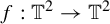
Theorem A. Let
$f:\mathbb {T}^2\to \mathbb {T}^2$
 be a
$C^1$
 -smooth DA endomorphism with a hyperbolic linearization
$A:\mathbb {T}^2\to \mathbb {T}^2$
 . If f is special, then it is semi-conjugate to A.
Remark 1.3. The proofs of Theorem A and the following results in this section need the dynamical coherence, that is, the center bundle on the universal cover space is integrable. DA endomorphisms on
$\mathbb {T}^2$
 are actually dynamically coherent [Reference Hall and Hammerlindl27], see also [Reference He, Shi and Wang33] in the setting of absolutely partially hyperbolic endomorphisms (see the definition in §2.1) on
$\mathbb {T}^2$
 . However, it is still unknown if it holds or not for the high-dimensional case. Indeed, for DA diffeomorphisms or absolutely partially hyperbolic diffeomorphisms, there are similar results on
$\mathbb {T}^3$
 and open questions on
$\mathbb {T}^d\ (d\geqslant 4)$
 [Reference Brin, Burago and Ivanov6, Reference Fisher, Potrie and Sambarino15, Reference Potrie48, Reference Rodriguez Hertz, Rodriguez Hertz and Ures54].
It seems that the special property is also a necessary condition for the existence of semi-conjugacy, because it is true for the Anosov case, as mentioned above. Indeed, considering a non-special Anosov endomorphism f on
$\mathbb {T}^2$
 , there is a point x with at least two transverse unstable manifolds
$\mathcal {F}^u_1(x)$
 and
$\mathcal {F}^u_2(x)$
 [Reference Przytycki49]. If f is conjugate via h to its linearization A, h will map
$\mathcal {F}^u_1(x)$
 and
$\mathcal {F}^u_2(x)$
 to the unstable manifold of A at
$h(x)$
 . It contradicts the fact that h is a homeomorphism. However, this trick does not work for semi-conjugacy or DA endomorphisms.
In addition to the difference between Anosov endomorphisms and DA endomorphisms, there is an interesting observation restricted to the context of DA endomorphisms.
-
• When a DA endomorphism admits a stable bundle (that is, it is uniformly contracting on a subbundle), called sc-DA (see the definition in §2.1.2), by a similar argument to the Anosov case, it can be easily shown that the semi-conjugacy guarantees the special property, see Corollary 2.10.
-
• When a DA endomorphism admits an unstable cone-field (that is, it is uniformly expanding on a cone-field), called cu-DA (see also §2.1.2), the proof will be much more complicated. Indeed, the study of the $cu$
 -DA endomorphism needs an intuitively stronger rigidity of the semi-conjugacy as follows: the existence of semi-conjugacy between f and its linearization implies that the center Lyapunov exponents of f on the periodic points coincide with its linearization.

Then, we conclude that a DA endomorphism (for both cases of
$sc$
 -DA and
$cu$
 -DA) is semi-conjugate to its linearization if and only if it is special.
1.2 Rigidity of the semi-conjugacy
The rigidity issue in smooth dynamics focuses on the phenomenon that ‘weak equivalence implies strong equivalence’. A typical type of rigidity question is the following. Let Anosov local diffeomorphisms
$f,g:M\to M$
 be conjugate via a homeomorphism
$h:M\to M$
 , that is,
$h\circ f=g\circ h$
 . It is clear that a necessary condition of h being smooth is the matrices
$Df^{\pi (p)}(p)$
 and
$Dg^{\pi (p)}(h(p))$
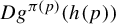 being conjugate for every periodic point p of f with period
$\pi (p)$
 . The rigidity means that such a necessary condition is also sufficient for the conjugacy h being smooth. In addition to matching the derivatives of return maps at periodic points, one can also consider more necessary conditions of the smooth conjugacy h, such as matching other periodic data (the Lyapunov exponents or Jacobian), matching the Lyapunov exponents with respect to the volume, and so on. There are many results on this type of rigidity, e.g., [Reference Cantarino and Varão8, Reference de la Llave13, Reference de la Llave14, Reference Gogolev19, Reference Gogolev and Rodriguez Hertz23, Reference Micena41, Reference Saghin and Yang56].
In this subsection, we will see that the semi-conjugacy guarantees partially matching periodic data. For DA endomorphisms on
$\mathbb {T}^2$
 , we will present the rigidity that the existence of the semi-conjugacy on the torus imposes on the non-invertible dynamics, with respect to the two cases of Mañé-type:
$cu$
 -DA and
$sc$
 -DA. Actually, the study of the differences between these two types of DA endomorphisms seems to be a subject of independent interest as well.
For the DA endomorphisms with unstable cone-fields, we have the following result. Denote by Per
$(f)$
 the periodic points set of f and
$\unicode{x3bb} ^s(p,f)$
 the stable Lyapunov exponent at
$p\in \mathrm {Per}(f)$
 .
Theorem B. Let
$f:\mathbb {T}^2\to \mathbb {T}^2$
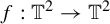 be a
$C^{1}$
 -smooth
$cu$
 -DA endomorphism semi-conjugate to its hyperbolic linearization
$A:\mathbb {T}^2\to \mathbb {T}^2$
 . Then, f is a special Anosov endomorphism. In particular, the semi-conjugacy is an injection; hence, the semi-conjugacy is a topological conjugacy. Moreover,
$\unicode{x3bb} ^s(p,f)=\unicode{x3bb} ^s(A)$
 for any
$p\in \mathrm {Per}(f)$
 .
Remark 1.4. The recent work about the rigidity of Anosov endomorphisms on the existence of topological conjugacy [Reference An, Gan, Gu and Shi1] shows that a
$C^{1+}$
 -smooth Anosov endomorphism g on
$\mathbb {T}^2$
 is conjugate to its linearization A if and only if g is special if and only if its stable Lyapunov exponents at periodic points are the same as A. In particular, the
$C^{1+}$
 -regularity assumption is used only for proving that the constant periodic stable Lyapunov exponent implies the existence of conjugacy and the special property. A key tool in [Reference An, Gan, Gu and Shi1] is the A-preimage set of every point becoming dense exponentially, see Lemma 2.3. Note that g inherits this property, since the conjugacy is in fact Hölder continuous [Reference Katok and Hasselblatt35]. However, the semi-conjugacy relating f and A in Theorem B is a priori non-injective. In addition, the method in the present paper is more general.
For the DA endomorphisms with stable subbundles, we have the following result.
Theorem C. Let
$f:\mathbb {T}^2\to \mathbb {T}^2$
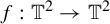 be a
$C^1$
 -smooth
$sc$
 -DA endomorphism semi-conjugate to its hyperbolic linearization
$A:\mathbb {T}^2\to \mathbb {T}^2$
 via a surjection
$h:\mathbb {T}^2\to \mathbb {T}^2$
 . Then, f is special. Moreover, the closure of h-injective points set

is invariant and satisfies:
-
(1) $\overline {\mathrm {Per}(f|_{\Lambda })}=\Lambda $
; -
(2) $\unicode{x3bb} ^s(p,f)=\unicode{x3bb} ^s(A)$
for any
$p\in \mathrm {Per}(f|_{\Lambda })$
.



Remark 1.5. There is also motivation for the investigation of
$sc$
 -DA endomorphisms for their relation to multivalued expanding mappings on branched manifolds. We refer to [Reference Przytycki50, p. 76].
Moreover, related to the result of
$sc$
 -DA endomorphisms, we also have the following proposition indicating the non-negligible gap between the semi-conjugacy and topological conjugacy.
Proposition D. For any Anosov endomorphism
$A:\mathbb {T}^2\to \mathbb {T}^2$
 , there exists a
$C^\infty $
 -smooth
$sc$
 -DA endomorphism
$g_0:\mathbb {T}^2\to \mathbb {T}^2$
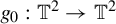 semi-conjugate to A such that every semi-conjugacy
$h:\mathbb {T}^2\to \mathbb {T}^2$
 homotopic to
$\mathrm {Id}_{\mathbb {T}^2}$
 is indeed non-injective.
Combining the results above, we have some reformulations. Precisely, Theorems A and B imply the following corollary. Note that when f is special, there will be a natural way to define the map
$h:\mathbb {T}^2\to \mathbb {T}^2$
 as the projection of a priori semi-conjugacy between the lifted maps on
$\mathbb {R}^2$
 .
Corollary E. Let
$f:\mathbb {T}^2\to \mathbb {T}^2$
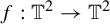 be a
$C^{1+\alpha }$
 -smooth
$cu$
 -DA endomorphism and
${A:\mathbb {T}^2\to \mathbb {T}^2}$
 be its hyperbolic linearization. Then, the following are equivalent:
-
(1) f is semi-conjugate to A via $h:\mathbb {T}^2\to \mathbb {T}^2$
; -
(2) f is conjugate to A via $h:\mathbb {T}^2\to \mathbb {T}^2$
; -
(3) f is special;
-
(4) f is Anosov and $\unicode{x3bb} ^s(p,f)=\unicode{x3bb} ^s(A)$
for any
$p\in \mathrm {Per}(f)$
.




In particular, each of them implies that the conjugacy h is
$C^{1+\alpha }$
 -smooth along the stable foliation.
Remark 1.6. We require
$C^{1+\alpha }$
 -regularity of f in Corollary E. In particular, for proving ‘(4)
$\implies $
 (1),(2),(3)’ and the smoothness of h, we will apply the main result of [Reference An, Gan, Gu and Shi1] mentioned in Remark 1.4, where it needs the
$C^{1+}$
 -smoothness to apply the Livšic theorem (see [Reference An, Gan, Gu and Shi1, §§4 and 5] for more details).
Remark 1.7. An interesting rigidity result in Corollary E is that if the semi-conjugacy exists, it is actually a conjugacy and smooth along the stable foliation. Such a phenomenon as lower-regularity automatically implying higher-regularity is usually called ‘bootstrap’. To see recent works on bootstrap, we refer to [Reference Gogolev20, Reference Kalinin, Sadovskaya and Wang34] for Anosov diffeomorphisms, [Reference Gogolev, Kalinin and Sadovskaya21] for partially hyperbolic diffeomorphisms, and [Reference Gogolev and Rodriguez Hertz22] for Anosov flows.
From Theorems A and C, we have the following corollary immediately.
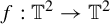
Corollary F. Let
$f:\mathbb {T}^2\to \mathbb {T}^2$
 be a
$C^{1}$
 -smooth
$sc$
 -DA endomorphism and
${A:\mathbb {T}^2\to \mathbb {T}^2}$
 be its hyperbolic linearization. Then, the following are equivalent:
-
(1) f is semi-conjugate to A via $h:\mathbb {T}^2\to \mathbb {T}^2$
; -
(2) f is special.

In particular, each of them implies that the closure of h-injective points set

is invariant and satisfies
-
(1) $\overline {\mathrm {Per}(f|_{\Lambda })}=\Lambda $
; -
(2) $\unicode{x3bb} ^s(p,f)=\unicode{x3bb} ^s(A)$
for any
$p\in \mathrm {Per}(f|_{\Lambda })$
.



Comparing this result with Corollary E, there are the following remark and question.
Remark 1.8. Based on Proposition D, we further give an example of
$sc$
 -DA endomorphism with periodic stable Lyapunov exponents being the same as its linearization on an invariant set saturated by the stable foliation, but it is not semi-conjugate to its linearization (see Proposition 5.1).
Question 1.9. Under the assumption of Corollary F, it is known that h preserves the stable foliation and is a homeomorphism restricted to each stable leaf (see Proposition 2.7). There is still a question whether the semi-conjugacy is smooth along each stable leaf or not. Note that even if f is
$C^2$
 , there is no Livšic theorem [Reference Livšic37] in this situation, which is important to the rigidity issue when one wants to get the smoothness of the conjugacy from the periodic data, see for example [Reference An, Gan, Gu and Shi1, Reference de la Llave14, Reference Gogolev19].
1.3 Applications for the volume-preserving case
In what follows, we would like to give some applications. Recall that Theorem B implies that a special
$cu$
 -DA endomorphism must be Anosov, while Proposition D asserts that a special
$sc$
 -DA endomorphism may not have to be Anosov. A direct reason behind this difference is that the injective points set
$\Lambda $
 in Theorem C may not be hyperbolic for the
$sc$
 -DA case, while it must be hyperbolic in the setting of
$cu$
 -DA (see Lemma 6.1 and Remark 6.3 for more details). Thus, to show more rigidity for the
$sc$
 -DA case, we introduce some assumptions to control the dynamics on the center direction, in particular, we focus on the volume-preserving condition.
In this paper,
$f:\mathbb {T}^2\to \mathbb {T}^2$
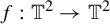 is called volume-preserving if f admits an invariant smooth measure m, that is, the density
$\rho :\mathbb {T}^2\to \mathbb {R}_+$
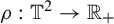 of m is smooth, with
$dm=\rho d\mathrm {Leb}$
 and
$\mathrm {Leb}$
 is the Lebesgue measure of
$\mathbb {T}^2$
 . Such a measure m will be referred to as a smooth volume measure.
First, parallel to Corollary E, we have the following result as a corollary of Theorem C.
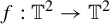
Corollary G. Let
$f:\mathbb {T}^2\to \mathbb {T}^2$
 be a
$C^{1+\alpha }$
 -smooth
$sc$
 -DA endomorphism and
${A:\mathbb {T}^2\to \mathbb {T}^2}$
 be its hyperbolic linearization. If f is volume-preserving, then the following are equivalent:
-
(1) f is semi-conjugate to A via $h:\mathbb {T}^2\to \mathbb {T}^2$
; -
(2) f is conjugate to A via $h:\mathbb {T}^2\to \mathbb {T}^2$
; -
(3) f is special;
-
(4) f is Anosov and $\unicode{x3bb} ^s(p,f)=\unicode{x3bb} ^s(A)$
for any
$p\in \mathrm {Per}(f)$
.




In particular, each of the items implies that the conjugacy h is
$C^{1+\alpha }$
 -smooth along the stable foliation.
Remark 1.10. As we mentioned in Remark 1.6, the only two parts of Corollary G requiring
$C^{1+\alpha }$
 -regularity are ‘(4)
$\implies $
 (1),(2),(3)’ and the smoothness of h.
So, the
$sc$
 -DA case (Corollary G) and the
$cu$
 -DA case (Corollary E) can be unified in the volume-preserving setting. Moreover, since a
$C^{1+\alpha }$
 volume-preserving Anosov endomorphism is ergodic [Reference Micena and Tahzibi42], as an immediate corollary, we also obtain the ergodicity of DA endomorphisms as follows.
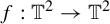
Corollary H. Let
$f:\mathbb {T}^2\to \mathbb {T}^2$
 be a special
$C^{1+\alpha }$
 -smooth DA endomorphism. If f is volume-preserving, then it is ergodic with respect to the volume measure.
Question 1.11. Is a
$C^{1+\alpha }$
 -smooth volume-preserving DA endomorphism on
$\mathbb {T}^2$
 ergodic with respect to the volume without the special assumption? Note that a volume-preserving
$C^{1+\alpha }$
 -smooth DA diffeomorphism g on
$\mathbb {T}^3$
 is always special and semi-conjugate to its linearization, so Corollary H can be seen as an analogue of the main results of [Reference Gan and Shi18, Reference Hammerlindl and Ures32] in the non-invertible case.
Finally, we consider special DA endomorphisms with the same periodic Jacobian as the linearizations. We can get that these DA endomorphisms are smoothly conjugate to their linearization. We refer to [Reference Gogolev and Rodriguez Hertz23] for a Jacobian rigidity result for expanding maps, where the authors introduce a method called ‘matching function’ (see also [Reference Gogolev and Rodriguez Hertz22] for details of this technique) that is not used for the endomorphism case here. For
$r>1$
 , denote by

Corollary I. Let
$f:\mathbb {T}^2\to \mathbb {T}^2$
 be a
$C^r$
 -smooth
$(r>1)$
 DA endomorphism. Assume that f is semi-conjugate to its hyperbolic linearization A, and for any
$n\in \mathbb {N}$
 and
${p\in \mathrm {Fix}(f^n)}$
 ,

Then, f is a volume-preserving Anosov endomorphism and
$C^{r_*}$
 -conjugate to A.
Remark 1.12. It is known that when g is a
$C^{1+\alpha }$
 transitive Anosov diffeomorphism, g admitting an invariant measure that is absolutely continuous with respect to Lebesgue measure is equivalent to g having the same periodic Jacobian as its linearization [Reference Bowen5, Theorem 4.14]. However, for
$C^{1+\alpha }$
 transitive Anosov endomorphisms, these two conditions are not equivalent in general. In fact, when f is a transitive and non-invertible Anosov endomorphism, the Jacobian condition will lead to an invariant measure with Hölder density by the same method as [Reference Bowen5, Theorem 4.14] employing Livšic theorem. However, the converse is not true, even if f preserves a smooth measure. In addition, we give a counterexample in Example 7.5.
1.4 Comparison with the case of DA diffeomorphisms
Other main motivations of this paper are inspired by several interesting results for DA diffeomorphisms on
$\mathbb {T}^3$
 [Reference Gan and Shi18, Reference Hammerlindl and Shi31, Reference Hammerlindl and Ures32] and the related differences (also similarities) corresponding to the case of DA endomorphisms. Here, we would like to make them more clear.
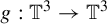
Let
$g:\mathbb {T}^3\to \mathbb {T}^3$
 be a
$C^{1+\alpha }$
 -smooth DA diffeomorphism with a partially hyperbolic splitting
$T\mathbb {T}^3=E^s_g\oplus E^c_g\oplus E^u_g$
 , and
$L:\mathbb {T}^3\to \mathbb {T}^3$
 be its hyperbolic linearization with a partially hyperbolic splitting
$T\mathbb {T}^3=L^{ss}\oplus L^{cs}\oplus L^u$
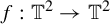
 . Let
$f:\mathbb {T}^2\to \mathbb {T}^2$
 be a DA endomorphism with linear part A.
-
(1) In [Reference Hammerlindl and Ures32], Hammerlindl and Ures proved that if g is volume-preserving (or transitive) and $su$
-integrable, namely, the bundles
$E^s_g$
and
$E^u_g$
are jointly integrable, then it is topologically conjugate to L. This phenomenon is similar to ‘
$(3) \Rightarrow (2)$
’ of both Corollaries E and G if one sees the special property as the integrability of the dominating direction
$E^2_f$
(for definition, see (2.4)) joint with the direction induced by the generation set $$ \begin{align*}P(x)=\{y\in\mathbb{T}^2\mid f^k(y)=f^k(x)\ \mathrm{for}\ \mathrm{some}\ k\in\mathbb{N}\}.\end{align*} $$
It is worth mentioning that this set $P(x)$
can be regarded as the strong stable ‘leaf’ of x. However, in Corollary E, we will not assume that f is volume-preserving or transitive. -
(2) In [Reference Gan and Shi18], Gan and Shi proved that if g is $su$
-integrable and conjugate to L, then g is Anosov and its periodic points admit the same center Lyapunov exponents as L. This result has the same taste as Theorems B and C if one keeps seeing
$P(x)$
as the strong stable ‘leaf’ of f. However, we would not assume that f is special (corresponding to the
$su$
-integrability of g) in advance or there is a conjugacy between f and A. Here, we only need a semi-conjugacy on the torus that always exists in the case of DA diffeomorphisms. -
(3) In [Reference Hammerlindl and Shi31], Hammerlindl and Shi further proved that the existence of $su$
-leaves of g, in fact the boundaries of open
$su$
-accessible classes, implies that g is Anosov and admits the same periodic center Lyapunov exponents as L. Comparing with [Reference Gan and Shi18], there need not be a priori the existence of conjugacy or
$su$
-integrability on the whole
$\mathbb {T}^3$
. Here, in Theorems B and C, the semi-conjugacy between f and A actually guarantees that there is some submanifold (not a priori the ambient manifold) that is tangent to the dominating direction
$E^2_f$
and independent of the negative orbits, see also Corollary 2.10 and Proposition 2.11.


We also point out that the
$C^{1+\alpha }$
 -regularity of g is necessary in the proofs of [Reference Gan and Shi18, Reference Hammerlindl and Shi31, Reference Hammerlindl and Ures32]. However, the
$C^1$
 -regularity is enough for most results in the present paper, except for:
-
• applying the Livšic theorem to get that the constant periodic stable Lyapunov exponent of f implies f is special in Corollaries E and G, and to show the smoothness of the conjugacy in Corollaries E, G, and I;
-
• applying the Hopf’s argument to prove the ergodicity in Corollary H.
Finally, considering the special property as a kind of joint integrability, we concentrate on its rigidity. Based on the work of [Reference Gan and Shi18], Gogolev and Shi [Reference Gogolev and Shi24] recently extend a wide range of the rigidity on integrability in the setting of Anosov diffeomorphisms on higher-dimensional tori. In addition to the hyperbolic case, there are also works on the rigidity of integrability for partially hyperbolic diffeomorphisms [Reference Avila and Viana3, Reference Rodriguez Hertz52]. Let us explain more about them for comparison with our results here.
Let
$L:\mathbb {T}^4\to \mathbb {T}^4$
 be a totally irreducible automorphism with exactly two eigenvalues of absolute value one. Then, there is no Franks’ semi-conjugacy in this partially hyperbolic situation either. Applying the Kolmogorov–Arnold–Moser (KAM) technique, Rodriguez Hertz [Reference Rodriguez Hertz52] shows that for a
$C^{22}$
 -small perturbation g, which is also partially hyperbolic, if g is
$su$
 -integrable, then g is topologically conjugate to L and the conjugacy is smooth along the center foliation. Note that this result could be compared with Corollary E. In the symplectic setting, Avila and Viana [Reference Avila and Viana3] show that the
$su$
 -integrability implies a volume-preserving conjugacy between g and L by using the invariance principle. Corollary I displays a similar phenomenon if one replaces the equivalent condition of semi-conjugacy by the special property. We do not use the KAM theory and the invariance principle in our proofs.
1.5 Organization of this paper
The rest of the paper will be organized as follows. In §2, we collect some definitions and facts about DA endomorphisms on
$\mathbb {T}^2$
 and show directly that the existence of the semi-conjugacy h on
$\mathbb {T}^2$
 implies the integrability of the center. Meanwhile, we describe the structure of h-injective points for further preparation. Next, we prove Theorem A in §3 by showing the existence of a semi-conjugacy that commutes with deck transformations on
$\mathbb {R}^2$
 . The rigidity results implied by the existence of the semi-conjugacy on
$\mathbb {T}^2$
 will be obtained in two steps. In §4, we analyze the periodic data inside the closure of h-injective points set for both cases of
$sc$
 -DA and
$cu$
 -DA in an almost unified manner, see Proposition 4.1 for the main rigidity of Lyapunov exponents. For the case of
$sc$
 -DA, we continue to complete the proofs of Theorem C in §5, while we also give the counterexamples mentioned in Proposition D and Remark 1.8. In §6, we present the proofs of Theorem B and Corollary E for the
$cu$
 -DA case by showing the existence of negative center Lyapunov exponents. Finally, we prove Corollary G and Corollary I in §7 with extended discussions on the volume-preserving systems.
2 Preliminaries
2.1 Partial hyperbolicity
It is natural for endomorphisms to define partial hyperbolicity in terms of cone families. Let f be an endomorphism on a compact Riemannian manifold M. For a continuous bundle splitting
$TM=E_1\oplus E_2$
 and a constant
$\alpha>0$
 , there are two related cone-fields
$\mathcal {C}^{E_1}_\alpha $
 and
$\mathcal {C}^{E_2}_\alpha $
 defined by

A continuous splitting (may not be
$Df$
 -invariant)
$TM={E_1}\oplus {E_2}$
 is called a dominated splitting of f denoted by
$TM={E_1}\oplus _{<} {E_2}$
 if there are constants
$\alpha>0$
 and
$k\in \mathbb {N}$
 such that

where the interior of a cone
$\mathrm {int}(\mathcal {C}^{E_2}_{\alpha }(x))=\{ v\in T_xM\mid v=(v^{E_1},v^{E_2}),|v^{E_1}|<\alpha |v^{E_2}|\}\cup \{0_x\}$
 . Note that (2.1) also allows us to assume that
$E_1$
 is
$Df$
 -invariant (see for example [Reference Crovisier and Potrie12, Reference Hall and Hammerlindl27] or (2.3)).
Moreover, an endomorphism f is called partially hyperbolic if there exist a dominated splitting
$TM={E_1}\oplus _< {E_2}$
 , and constants
$\alpha>0$
 and
$k\in \mathbb {N}$
 such that

for any
$x\in M$
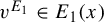
 , and unit vectors
$v^{E_1}\in E_1(x)$
 and
$v^{E_2}\in \mathcal {C}^{E_2}_\alpha (x)$
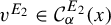 . In particular, there are two cases.
-
• We call f an $sc$
-partially hyperbolic endomorphism if the first inequality of (♦) holds. In this case, the cone-fields
$\mathcal {C}^{E_1}_\alpha $
and
$\mathcal {C}^{E_2}_\alpha $
will be called the stable cone-field and center cone-field, respectively. -
• We call f a $cu$
-partially hyperbolic endomorphism if the second inequality of (♦) holds. In this case, the cone-fields
$\mathcal {C}^{E_1}_\alpha $
and
$\mathcal {C}^{E_2}_\alpha $
will be called the center cone-field and unstable cone-field, respectively.


Remark 2.1. There are some remarks on the definition of partially hyperbolic endomorphisms involving the cone-field language. We refer the readers to [Reference Crovisier and Potrie12, §2] for more details.
-
(1) The domination (2.1) is equivalent to the existence of constants $\alpha>0$
and
$k\in \mathbb {N}$
satisfying (2.2) $$ \begin{align} |Df^k(v^{E_1})|< \tfrac{1}{2}|Df^k(v^{E_2})| \end{align} $$
for all $x\in M$
, and unit vectors
$v^{E_1}\in {E_1}(x)$
and
$v^{E_2}\in \mathcal {C}^{E_2}_\alpha (x)$
. -
(2) As usual, one can also define the partial hyperbolicity by choosing constants $C>1$
and
$0<\unicode{x3bb} <1$
such that the domination $$ \begin{align*}|Df^n(v^{E_1})|\leqslant C\unicode{x3bb}^n |Df^n(v^{E_2})|\quad\text{for all}\ n\in \mathbb{N},\end{align*} $$
and the hyperbolicity
$$ \begin{align*} |Df^n(v^{E_1})|\leqslant C\unicode{x3bb}^n \quad \mathrm{or} \quad |Df^n(v^{E_2})|\geqslant C^{-1}\unicode{x3bb}^{-n}\quad \text{for all}\ n\in \mathbb{N}, \end{align*} $$
holds for any $x\in M$
, and unit vectors
$v^{E_1}\in {E_1}(x)$
and
$v^{E_2}\in \mathcal {C}^{E_2}_\alpha (x)$
. This definition is equivalent to inequalities of (2.2) and (♦), up to taking k via
$(C,\unicode{x3bb} )$
or vice versa. -
(3) The definition of partial hyperbolicity is independent of the metric in the sense that another equivalent metric will just lead to different constants $\alpha $
(the size of cone-fields) and
$k\in \mathbb {N}$
.


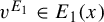


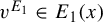
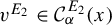


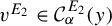
Furthermore, we call f an absolutely partially hyperbolic endomorphism if it is partially hyperbolic and (2.2) holds for any
$x,y\in M$
 , and unit vectors
$v^{E_1}\in E_1(x)$
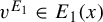 and
${v^{E_2}\in \mathcal {C}^{E_2}_\alpha (y)}$
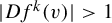
 . In particular, we call f an expanding endomorphism if it has trivial bundle
$E_1$
 in the dominated splitting, and there exists
$k\in \mathbb {N}$
 such that
$|Df^k(v)|>1$
 for any
$x\in M$
 and unit vector
$v\in T_xM$
 .
2.1.1 Special endomorphisms
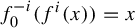
Note that there exists a
$Df$
 -invariant bundle
$E^1_f\subset \mathcal {C}^{E_1}_\alpha $
 given by

where
$f^{-i}_0(f^i(x))=x$
 . Similarly, for a given negative orbit
$\tilde {x}=(\ldots ,x_{-2},x_{-1},x)$
 of
$x\in M$
 , there is a
$Df$
 -invariant direction (along this orbit
$\tilde {x}$
 ) called the dominating direction,

We refer to [Reference Przytycki49] for more properties, such as the continuity of directions with respect to orbits.
It should be noticed that there are generally cone-fields
$\mathcal {C}^{E_2}_\alpha (x)$
 rather than
$Df$
 -invariant bundles that are independent of the negative orbits, unless the partially hyperbolic endomorphism is special.
Precisely, a partially hyperbolic endomorphism
$f:M\to M$
 is called special if there exists a
$Df$
 -invariant partially hyperbolic splitting

that is, the dominating direction of a point is independent of its negative orbits.
2.1.2 Derived from Anosov endomorphisms
If both of these inequalities in (♦) hold, f will be an Anosov endomorphism. A partially hyperbolic endomorphism f is called derived from Anosov (abbreviated DA endomorphism) if its linear part
$f_*$
 is an Anosov endomorphism. More precisely, there are the following cases corresponding to the two inequalities in (♦).
-
• When the DA endomorphism f is $sc$
-partially hyperbolic, we call f sc-DA. In this case, f admits a stable cone-field that, by (2.3), gives a
$Df$
-invariant uniformly contracting subbundle that will be called the stable bundle and is denoted by
$E^s_f$
. -
• When the DA endomorphism f is $cu$
-partially hyperbolic, we call f cu-DA. In this case, f admits an unstable cone-field and by (2.3), the center cone-field gives a
$Df$
-invariant subbundle that will be called the center bundle and is denoted by
$E^c_f$
.


2.2 Semi-conjugacy
Throughout this subsection, we use the following notation. Let
$f:\mathbb {T}^2\to \mathbb {T}^2$
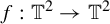 be a
$C^1$
 -smooth DA endomorphism and
$A:\mathbb {T}^2\to \mathbb {T}^2$
 be its linearization. Let
$F:\mathbb {R}^2\to \mathbb {R}^2$
 be a lift of f via
$\pi :\mathbb {R}^2\to \mathbb {T}^2$
 . In short, we still denote the lift of
${A:\mathbb {T}^2\to \mathbb {T}^2}$
 via
$\pi $
 by
$A:\mathbb {R}^2\to \mathbb {R}^2$
 . In addition, we denote the stable/unstable bundles and foliations of A by
$L^{s/u}$
 and
$\mathcal {L}^{s/u}$
 on
$\mathbb {T}^2$
 ,
$\widetilde {L}^{s/u}$
 and
$\widetilde {\mathcal {L}}^{s/u}$
 on
$\mathbb {R}^2$
 , respectively.
Recall that
$\mathcal {L}^{s/u}$
 is minimal, namely, for every
$x\in \mathbb {T}^2$
 , the leaf
$\mathcal {L}^{s/u}(x)$
 is dense in
$\mathbb {T}^2$
 . Then, there is the following property.
Proposition 2.2. For any
$x\in \mathbb {R}^2$
 and
$k\in \mathbb {N}$
 , the set

is dense in
$\mathbb {R}^2$
 , where
$\sigma =s,u$
 .
Proof. It suffices to verify for
$x=0$
 since the foliation
$\widetilde {\mathcal {L}}^{\sigma }$
 consists of translations of the leaf
$\widetilde {\mathcal {L}}^{\sigma }(0)$
 for
$\sigma =s,u$
 . Note that the lifted map of the linearization
$A:\mathbb {R}^2\to \mathbb {R}^2$
 is an Anosov diffeomorphism with no trivial bundles in the partially hyperbolic splitting. Thus, for a given
$k\in \mathbb {N}$
 , one can get
$A^k\{\widetilde {\mathcal {L}}^{\sigma }(0)+\mathbb {Z}^2\}$
 is dense in
$\mathbb {R}^2$
 . Then, it follows that the set
$\{\widetilde {\mathcal {L}}^{\sigma }(0+A^k\mathbb {Z}^2)\}$
 is dense in
$\mathbb {R}^2$
 .
Focusing on the A-preimage set, there is the following useful estimate.
Lemma 2.3. [Reference An, Gan, Gu and Shi1, Proposition 2.10]
There exist
$C_A>0$
 and
$0<\gamma <1$
 such that for any
$x\in \mathbb {T}^2$
 ,
$k\in \mathbb {N}$
 , the k-preimage set of x,

is
$C_A\cdot \gamma ^k$
 -dense in
$\mathbb {T}^2$
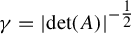
 . Here, one can take
$\gamma = {|}{\det} (A)|^{-\tfrac 12}$
 .
Remark 2.4. When
${|}{\det} (A)|=1$
 , the conclusion obviously holds for large constant
$C_A$
 . The interesting case of this lemma is
${|}{\det} (A)|>1$
 , which is exactly applicable to the linearization of DA endomorphism with which we are concerned in this paper.
2.2.1 The semi-conjugacy and foliations on the universal cover
There are some basic facts for the dynamics on the universal cover, especially, some properties related to the semi-conjugacy.
We first include the following classical result for toral endomorphisms.
Proposition 2.5. [Reference Aoki and Hiraide2, Theorem 8.2.1]
Let F and A be as in §2.2. There exists a unique surjection
$H:\mathbb {R}^2\to \mathbb {R}^2$
 satisfying the following:
-
(1) $H\circ F=A\circ H$
; -
(2) H is uniformly continuous;
-
(3) there exists $C_H>0$
such that
$\| H-\mathrm {Id}_{\mathbb {R}^2} \|_{C^0}<C_H$
.



Then, we collect useful properties for the semi-conjugacy on
$\mathbb {R}^2$
 . These properties of DA endomorphisms are adaptations of those of DA diffeomorphisms, Anosov endomorphisms, and
$cu$
 -DA endomorphisms in [Reference An, Gan, Gu and Shi1, Reference Hall and Hammerlindl27–Reference Hammerlindl29, Reference Hammerlindl and Shi31]. For completeness, we give proofs briefly based on the original ones.
We start by introducing some notation for the following results. For the map
${T_n:\mathbb {R}^2\to \mathbb {R}^2}$
 with
$T_n(x)=x+n$
 , we say H commutes with the deck transformations if

Note that the semi-conjugacy in Proposition 2.5 may not commute with the deck transformations; otherwise, it can descend to
$\mathbb {T}^2$
 and induce a semi-conjugacy between f and A.
The map
$T_{-n}\circ H\circ T_n$
 still keeps some good properties, for instance, it preserves the stable foliation and has the following asymptotic behavior.
Proposition 2.6. [Reference An, Gan, Gu and Shi1]
Let H and
$C_H$
 be as in Proposition 2.5. Then:
-
(1) for any $x\in \mathbb {R}^2$
and
$n\in \mathbb {Z}^2$
,
$H(x+n)-n\in \widetilde {\mathcal {L}}^s(H(x))$
; -
(2) for any $x\in \mathbb {R}^2$
,
$k\in \mathbb {N}$
, and
$n^*\in A^k\mathbb {Z}^2$
, one has $$ \begin{align*} | H(x+n^*)-H(x)-n^* |<2C_H\cdot \|A|_{L^s}\|^k. \end{align*} $$





Proof. By Proposition 2.5, one has
$\| H-\mathrm {Id}_{\mathbb {R}^2} \|_{C^0}<C_H$
 . Then, for any
$k\in \mathbb {N}$
 ,

where d is the natural Euclidean distance on
$\mathbb {R}^2$
 . This uniform upper bound indicates that there is no ‘unstable component’ for the difference between
$H(x+n)-n$
 and
$H(x)$
 , that is, they are in the same stable leaf for any
$n\in \mathbb {Z}^2$
 .
Moreover, for any
$n^*\in A^k\mathbb {Z}^2$
 , one has

so
$H (F^{-k}(x)+A^{-k}(n^*))$
 and
$H\circ F^{-k}(x)+A^{-k}(n^*)$
 are in the same stable leaf. Note that

Hence, one can get

Note that f is a partially hyperbolic endomorphism if and only if F is a partially hyperbolic diffeomorphism, by a similar argument to the Anosov case in [Reference Mañé and Pugh39]. Hence, the lifted diffeomorphism
$F:\mathbb {R}^2\to \mathbb {R}^2$
 admits an invariant partially hyperbolic splitting

One can also get the invariant splitting (2.6) by lifting the cone-fields of f to
$T\mathbb {R}^2$
 , and using the formulas similar to (2.4) and (2.3).
If f is
$sc$
 -DA, then
$DF$
 is contracting on
$E^1$
 ; meanwhile,
$E^1$
 is uniquely integrable. We denote the integral foliation on
$\mathbb {R}^2$
 by
$\mathcal {F}_F^s$
 , the stable foliation. Similarly, if f is
$cu$
 -DA, we can define the unstable foliation
$\mathcal {F}_F^u\subset \mathbb {R}^2$
 , which is tangent to the expanding bundle
$E^2$
 . We call
$\mathcal {F}_F^{s}$
 and
$\mathcal {F}_F^{u}$
 the hyperbolic foliations, which are the stable and unstable foliations in the cases of
$sc$
 -DA and
$cu$
 -DA, respectively. We refer to [Reference Pesin45] for the unique integrability of these hyperbolic foliations on
$\mathbb {R}^2$
 .
Two cases are a little different for the situation on
$\mathbb {T}^2$
 . The stable foliation
$\mathcal {F}^s_f$
 of
$sc$
 -DA always exists and is the projection of
$\mathcal {F}^s_F$
 . However, the unstable foliation
$\mathcal {F}^u_f$
 for a
$cu$
 -DA f exists only if f is special.
Following the works of leaf conjugacy by Hammerlindl [Reference Hammerlindl28, Reference Hammerlindl29], we know the lifted diffeomorphism
$F:\mathbb {R}^2\to \mathbb {R}^2$
 is dynamically coherent (without a priori quasi-isometric property). Moreover, we have some common propositions for the cases of
$sc$
 -DA and
$cu$
 -DA as follows.
Notation. The following notation includes upper indexes
$*^s,*^2$
 for
$sc$
 -DA and
$*^1,*^u$
 for
$cu$
 -DA when we emphasize the hyperbolic part, and only include upper indices
$*^1,*^2$
 for DA systems when we only point out the domination on
$\mathbb {R}^2$
 .
Proposition 2.7. [Reference Hall and Hammerlindl27, Reference Hammerlindl29]
The bundle
$E^i$
 is uniquely integrable to a foliation
$\mathcal {F}^i$
 for
$i=1,2$
 . Denote the center foliation by
$\mathcal {F}^c_F$
 . Then, the following properties hold.
-
(1) $\mathcal {F}^1$
and
$\mathcal {F}^2$
admit the global product structure, that is, for any
$x,y\in \mathbb {R}^2$
, the manifold
$\mathcal {F}^1(x)$
intersects with
$\mathcal {F}^2(y)$
exactly once. -
(2) The foliation $\mathcal {F}^i$
is quasi-isometric, that is, there exist
$C_1,C_2>0$
such that $$ \begin{align*}d_{\mathcal{F}^i}(x,y)<C_1|x-y|+C_2 \quad \text{for all}\ x\in\mathbb{R}^2\ \text{and}\ y\in \mathcal{F}^i(x). \end{align*} $$


Proof. By [Reference Hall and Hammerlindl27], this proposition holds for the
$cu$
 -DA case. Specifically, the dynamical coherence follows from [Reference Hall and Hammerlindl27, Theorem A], the global product structure is given by [Reference Hall and Hammerlindl27, Proposition 2.12], and the quasi-isometry of the foliations
$\mathcal {F}^u_F$
 and
$\mathcal {F}^c_F$
 are respectively given by [Reference Hall and Hammerlindl27, Proposition 2.10(2)] and [Reference Hall and Hammerlindl27, Lemma 3.3].
Now, we consider the
$sc$
 -DA
$f:\mathbb {T}^2\to \mathbb {T}^2$
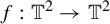 . The proofs for the dynamical coherence, the global product structure, and the quasi-isometry of the foliation
$\mathcal {F}^s_F$
 are similar to the proofs in [Reference Hall and Hammerlindl27]. Here, we briefly explain how it works for the
$sc$
 -DA case. Consider the inverse map
$F^{-1}:\mathbb {R}^2\to \mathbb {R}^2$
 of the lift of
$sc$
 -DA f. Note that
$F^{-1}$
 is a partially hyperbolic diffeomorphism with invariant unstable bundle and is semi-conjugate to the hyperbolic diffeomorphism
$A^{-1}:\mathbb {R}^2\to \mathbb {R}^2$
 . Since the argument in [Reference Hall and Hammerlindl27, Theorem A, Propositions 2.12, and 2.10(2)] are completely in the universal cover
$\mathbb {R}^2$
 , these properties hold for
$F^{-1}$
 and
$\mathcal {F}^{\,c/u}_{F^{-1}}$
 . Hence, we get that these properties also hold for F and
$\mathcal {F}^{\,s/c}_{F}$
 . Then, it remains to prove the quasi-isometry of
$\mathcal {F}^c_F$
 .
The quasi-isometry of
$\mathcal {F}^c_F$
 in the
$sc$
 -DA case is not as direct as above. Note that the proof of [Reference Hall and Hammerlindl27, Lemma 3.3], that is, the quasi-isometry of
$\mathcal {F}^c_F$
 in the
$cu$
 -DA case, needs
$\mathcal {F}^c_F$
 commuting with the
$\mathbb {Z}^2$
 -actions. This does not a priori hold in the
$sc$
 -DA case. However, combining the argument in [Reference Hammerlindl29, Reference Hall and Hammerlindl27],
$\mathcal {F}^c_F$
 is also quasi-isometric in the
$sc$
 -DA case. Note that though the paper [Reference Hammerlindl29] deals with the
$3$
 -nilmanifold case, the argument can be adapted for the
$2$
 -torus. We refer to the proof of [Reference Hall and Hammerlindl27, Proposition 2.10], where the authors of both [Reference Hall and Hammerlindl27, Reference Hammerlindl29] explain how the argument in [Reference Hammerlindl29] works for the
$2$
 -torus as well.
Now, we give a brief proof of the quasi-isometry of
$\mathcal {F}^c_F$
 in the
$sc$
 -DA case. Denote by
$\pi ^{s/u}:\mathbb {R}^2\to \widetilde {\mathcal {L}}^{s/u}(0)$
 the projections along foliations
$ \widetilde {\mathcal {L}}^{u/s}$
 . The following properties are immediate from [Reference Hall and Hammerlindl27, Reference Hammerlindl29] to the
$cu$
 -partially hyperbolic diffeomorphism
$F^{-1}$
 .
-
(1) ([Reference Hall and Hammerlindl27, Lemma 2.3], [Reference Hammerlindl29, Lemma 4.10]) There exists $R>0$
such that for any center segment
$J^c$
, the interval
$\pi ^s(J^c)$
has length at most R. (This can be done by using the argument in [Reference Hall and Hammerlindl27, Lemma 2.3] or [Reference Hammerlindl29, Lemma 4.10] for the
$cu$
-partially hyperbolic diffeomorphism
$F^{-1}$
.) -
(2) [Reference Hall and Hammerlindl27, Corollary 2.5] There exists $R>0$
such that for any stable segment
$J^s$
, the interval
$\pi ^u(J^s)$
has length at most R. (This can be done by using the argument in [Reference Hall and Hammerlindl27, Corollary 2.5] for the
$cu$
-partially hyperbolic diffeomorphism
$F^{-1}$
.) -
(3) ([Reference Hall and Hammerlindl27, Lemma 2.9], [Reference Hammerlindl29, Lemma 4.7]) For any $C>0$
, there exists
$l>0$
such that any center segment
$J^c$
of length greater than l is such that
$\pi ^u(J^c)$
has length greater than C. (This can be proved by the same proof of [Reference Hall and Hammerlindl27, Proposition 2.8 and Lemma 2.9], where one just needs to replace [Reference Hall and Hammerlindl27, Corollary 2.5] by the property given by the above item.)


Then, by modifying the proof of [Reference Hammerlindl29, Lemma 4.13], we can get the following claim.
Claim 2.8. For any
$M>0$
 , there exists
$l>0$
 such that any center segment
$J^c$
 of length greater than l has endpoints p and q with
$|\pi ^u(p)-\pi ^u(q)|>M$
 .
Proof. Let
$J^c$
 be a center curve with length great enough and
$\alpha :[0,1]\to \mathbb {R}^2$
 be its parameterization. Let R be as in items (1) and (2) above. Taking
$C=M+2R$
 and l in item (3) above, we get that there are
$s,t\in [0,1]$
 satisfying

Without loss of generality, we assume
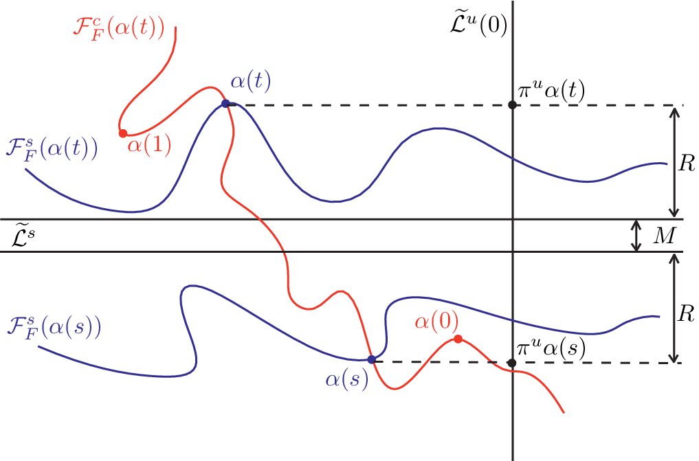
$s<t$
 (see Figure 1). Here, we identify
$\widetilde {\mathcal {L}}^u(0)$
 with
$\mathbb {R}$
 .
The projections of endpoints of
$J^c$
 on
$\widetilde {\mathcal {L}}^u$
 have distance bigger than M. (Color online.)

Figure 1 Long description
A line diagram on a white background featuring horizontal and vertical axes. A central horizontal band is bounded by two parallel black lines labeled tilde L super s on the left, with a vertical double-headed arrow inside labeled M. A vertical black line on the right is labeled tilde L super u (0).
In the upper region:
- A wavy blue curve labeled script F sub F super s (alpha(t)) spans the width.
- A red curve labeled script F sub F super c (alpha(t)) starts at a red dot alpha(1) and intersects the blue curve at a blue dot alpha(t).
- A horizontal dashed line extends from alpha(t) to the vertical axis at a black dot labeled pi super u alpha(t).
- A vertical double-headed arrow between this dashed line and the central band is labeled R.
In the lower region:
- A second wavy blue curve labeled script F sub F super s (alpha(s)) spans the width.
- The red curve continues downward, passing through a red dot alpha(0) and intersecting the lower blue curve at a blue dot alpha(s).
- A horizontal dashed line extends from alpha(s) to the vertical axis at a black dot labeled pi super u alpha(s).
- A vertical double-headed arrow between this dashed line and the central band is also labeled R.
By item (2), for any
$x\in \mathbb {R}^2$
 , the complement
$\mathbb {R}^2 \setminus \mathcal {F}^s_F(x)$
 has connected components
$B_-(x)$
 and
$B_+(x)$
 satisfying

Combining item (2) with the global product structure, we get that the curve
$\alpha ((t,1])$
 is located in the component
$B_+(\alpha (t))$
 of
$\mathbb {R}^2 \setminus \mathcal {F}^s_F(\alpha (t))$
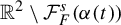 , namely,
$\alpha ((t,1])\subset B_+(\alpha (t))$
 . Hence, we have
$\alpha ((t,1])\subset \mathbb {R}^2\setminus H^{-}_R(\alpha (t))$
 , which implies
$\pi ^u\alpha (1)-\pi ^u\alpha (t)>-R$
 . Similarly, we have
$\alpha ([0,s))\subset \mathbb {R}^2\setminus H^{+}_R(\alpha (s))$
 , which implies
$\pi ^u\alpha (s)-\pi ^u\alpha (0)>-R$
 . Then, by (2.7), we get

This ends the proof of Claim 2.8.
Now, we show that Claim 2.8 is sufficient to get the quasi-isometry of
$\mathcal {F}^c_F$
 . Indeed, let constants M and l be as in Claim 2.8, and
$J^c$
 be a center curve with endpoints
$x,y$
 and with length
$L=kl+r$
 , where
$k\in \mathbb {N}$
 and
$0\leqslant r<l$
 . Then, by Claim 2.8,
${|\pi ^u(x)-\pi ^u(y)|\geqslant kM}$
 . Thus, there is a constant
$\beta>0$
 determined by the angle between
$\widetilde {\mathcal {L}}^s$
 and
$\widetilde {\mathcal {L}}^u$
 such that
$d(x,y)\geqslant k\beta M$
 . Then, for
$L\geqslant 2l$
 , one has
$L-r\geqslant {L}/{2}$
 and

Hence,
$d_{\mathcal {F}^c_F}(x,y)=L\leqslant ({2l}/{M\beta })d(x,y)$
 for
$L\geqslant 2l$
 . In particular, for any
$L>0$
 , one has

This concludes the quasi-isometry of
$\mathcal {F}^c_F$
 , and ends the proof of Proposition 2.7.
Now, we can get more information about the semi-conjugacy H restricted to the leaf of these foliations with the nice properties established above.
Proposition 2.9. [Reference Hall and Hammerlindl27, Reference Hammerlindl and Shi31]
Let H be as in Proposition 2.5. Then:
-
(1) the semi-conjugacy H maps $\mathcal {F}^1(x)$
and
$\mathcal {F}^2(x)$
onto
$\widetilde {\mathcal {L}}^s(H(x))$
and
$\widetilde {\mathcal {L}}^u(H(x))$
, respectively; -
(2) the semi-conjugacy H restricted to a hyperbolic leaf
$$ \begin{align*} H:\mathcal{F}_F^{s/u}(x) \to \widetilde{\mathcal{L}}^{s/u}(H(x)) \end{align*} $$is a homeomorphism, respectively;
-
(3) for any $x\in \mathbb {R}^2$
, the preimage
$H^{-1}(x)$
consists of either a single point or a compact segment inside a center leaf. Moreover, there exists a uniform upper bound for the length of
$H^{-1}(x)$
for every
$x\in \mathbb {R}^2$
.


Proof. It essentially follows the proof dealing with the
$cu$
 -DA case in [Reference Hall and Hammerlindl27], while the details in [Reference Hammerlindl and Shi31] for DA diffeomorphisms are strongly related as well. Just as in the last proposition, we briefly show the proof for the lifted
$sc$
 -DA map.
By the fact that the semi-conjugacy H is close to the identity and uniformly continuous, one can get H restricted to the hyperbolic leaf

is a homeomorphism. Then, according to the global product structure, it follows that H preserves the center leaf, and maps two distinct center leaves to the different lines in
$\widetilde {\mathcal {L}}^{u}$
 , namely, H is a bijection on the space of center leaves. Thus, H is surjective when restricted to center leaves.
Let us equip ‘
$\prec $
 ’ the order corresponding to the relative orientation on each leaf of
$\mathcal {F}^c_F$
 . Without loss of generality, we assume that F preserves this orientation. Now, we prove that the semi-conjugacy H is monotonic along center leaves. If not, taking
$x\prec y\prec z$
 along a center leaf
$J^c$
 with
$H(x)=H(z)\neq H(y)$
 , the forward iterates of A will expand the distances between
$H(y)$
 and
$H(x)$
 ,
$H(z)$
 . By the fact that H is a finite distance from the identity, one has

In addition, the order
$F^n(x)\prec F^n(y)\prec F^n(z)$
 implies

Using facts that center leaves are quasi-isometrically embedded and H is uniformly continuous,

which contradicts
$H(x)=H(z)$
 .
Based on the monotonicity of H along center leaves, for any
$x\in \mathbb {R}^2$
 , the non-empty set
$H^{-1}(x)$
 , which is a compact subset of some center leaf
$J^c$
 , will be connected; hence, it consists of either a single point or a compact segment inside the center leaf
$J^c$
 . Denote the two endpoints of
$H^{-1}(x)$
 by
$x_1$
 and
$x_2$
 . Since
$\mathcal {F}^c_F$
 is quasi-isometric (Proposition 2.7), one has

It follows from
$\|H-\mathrm {Id}_{\mathbb {R}^2}\|_{C^0}<C_H$
 that

Then, we obtain
$C\triangleq 2C_HC_1+C_2$
 , the uniform upper bound of the length of
$H^{-1}(x)$
 .
As a direct corollary, we can project the properties from those on the universal cover, when assuming the existence of a semi-conjugacy on
$\mathbb {T}^2$
 .
Corollary 2.10. Let
$f:\mathbb {T}^2\to \mathbb {T}^2$
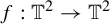 be a
$C^1$
 -smooth DA endomorphism and semi-conjugate to an Anosov endomorphism
$A:\mathbb {T}^2\to \mathbb {T}^2$
 via
$h:\mathbb {T}^2\to \mathbb {T}^2$
 . Then, f has the center bundle
$E^c_f\subset T\mathbb {T}^2$
 , which is uniquely integrable to the center foliation
$\mathcal {F}^c_f$
 . Moreover, for any
$x\in \mathbb {T}^2$
 , the preimage
$h^{-1}(x)$
 consists of either a single point or a compact segment with a uniformly upper bounded length inside the center leaf.
Proof. It suffices to prove the existence of the center bundle
$E^c_f$
 . If so, the unique integrability of
$E^c_f$
 and the property of
$h^{-1}$
 follow immediately from Propositions 2.7 and 2.9.
When f is
$cu$
 -DA, the existence of the
$Df$
 -invariant center bundle
$E^c_f$
 is guaranteed by iterating backward the center cone-field along positive orbits.
Now, let f be
$sc$
 -DA. Since f is semi-conjugate to A, the lifted semi-conjugacy
$H:\mathbb {R}^2\to \mathbb {R}^2$
 satisfies
$H(x+n)=H(x)+n$
 for any
$x\in \mathbb {R}^2$
 and
$n\in \mathbb {Z}^2$
 . Hence, one has

Since H is homeomorphic along
$\mathcal {F}^s_F$
 , it follows from the global product structure that

for any
$x\in \mathbb {R}^2$
 and
$n\in \mathbb {Z}^2$
 . Note that the center direction of f is continuous with respect to f-orbits, and the natural projection of the set of F-orbits is dense in
$\mathbb {T}^2_f$
 . Hence, one can get the existence of the
$Df$
 -invariant center bundle
$E^c_f$
 .
2.2.2 The set of injective points
Let H be as in Proposition 2.5. We now focus on preparing some technical properties for the set of injective points associated with the surjection H.
Throughout this subsection, we assume that
$f:\mathbb {T}^2\to \mathbb {T}^2$
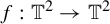 is semi-conjugate to
$A:\mathbb {T}^2\to \mathbb {T}^2$
 . Then, H commutes with the deck transformations. Denote by

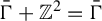
the semi-conjugacy between f and A. We define

and denote by
$\bar {\Gamma }$
 the closure of
$\Gamma $
 with respect to the topology of
$\mathbb {R}^2$
 .
By Corollary 2.10, the center foliation
$\mathcal {F}^c_f$
 exists and can be equipped with an order ‘
$\prec $
 ’ as well. Moreover, for any
$x\in \mathbb {T}^2$
 , we can define the endpoints of the set
$h^{-1}\circ h(x)$
 by
$x^-$
 and
$x^+$
 such that
$x^-\preceq x^+$
 , that is,
$x^-\prec x^+$
 or
$x^-=x^+$
 . Here,
$x^-=x^+$
 if and only if
$h^{-1}\circ h(x)=\{x\}$
 .
Following in the spirit of [Reference Hammerlindl and Shi31], we describe the structure of
$\bar {\Gamma }$
 as follows.
Proposition 2.11. [Reference Hammerlindl and Shi31]
Let H be as in Proposition 2.5. Assume H commutes with the deck transformations. Then, one has the following:
-
(1) $\bar {\Gamma }$
is
$F^{\pm 1}$
-invariant; -
(2) $\bar {\Gamma }+\mathbb {Z}^2=\bar {\Gamma }$
; in particular, the set
$\Lambda :=\pi (\bar {\Gamma })$
is
$f^{\pm 1}$
-invariant and (2.8) $$ \begin{align} \Lambda =\overline{\{x\in\mathbb{T}^2\mid h^{-1}\circ h(x)=\{x\}\}} =\bigcup_{x\in\mathbb{T}^2}\{x^+, x^-\}; \end{align} $$
-
(3) $\bar {\Gamma }$
is
$\mathcal {F}_F^{s/u}$
-saturated and
$f|_{\Lambda }$
is special; in particular,
$\Lambda $
is
$\mathcal {F}_f^{s}$
-saturated when f is
$sc$
-DA, and
$\Lambda $
is
$\mathcal {F}_f^{u}$
-saturated when f is
$cu$
-DA; -
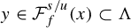
(4) given $x\in \Lambda $
, if
$x=x^{\sigma }$
, then
$y=y^{\sigma }$
for any
$y\in \mathcal {F}_f^{s/u}(x)\subset \Lambda $
and
$\sigma =+,-$
; -
(5) $\overline {\mathrm {Per}(f|_{\Lambda })}=\Lambda $
.






Proof. For the first item, let
$x\in \Gamma $
 . Then,

Hence,
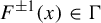
$F^{\pm 1}(x)\in \Gamma $
 . It follows from the continuity that
$\bar {\Gamma }$
 is
$F^{\pm 1}$
 -invariant.
For the second item, let
$x\in \Gamma $
 and
$n\in \mathbb {Z}^2$
 . We claim that
$H^{-1}\circ H(x+n)=\{x+n\}$
 . Indeed, let
$y\in H^{-1}\circ H(x+n)$
 , then
$H(y)=H(x+n)=H(x)+n$
 , that is,
${H(y-n)=H(x)}$
 . Since
$x\in \Gamma $
 , one has
$y=x+n$
 . Hence,
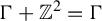
$\Gamma +\mathbb {Z}^2=\Gamma $
 and
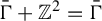
$\bar {\Gamma }+\mathbb {Z}^2=\bar {\Gamma }$
 .
Now, the set
$\Lambda :=\pi (\bar {\Gamma })$
 satisfies
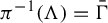
$\pi ^{-1}(\Lambda )=\bar {\Gamma }$
 and is
$f^{\pm 1}$
 -invariant by the first item. Indeed, let
$x\in \Lambda $
 . Then, as a set,
$f^{\pm 1}(x)=\pi \circ F^{\pm 1} \circ \pi ^{-1}(x)$
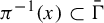
 . Since
$ \pi ^{-1}(x)\subset \bar {\Gamma }$
 and
$\bar {\Gamma }$
 is
$F^{\pm 1}$
 -invariant, one has
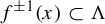
$F^{\pm 1} \circ \pi ^{-1}(x)\subset \bar {\Gamma }$
 and
$f^{\pm 1}(x)\subset \Lambda $
 .
Note that
$\Lambda =\pi (\bar {\Gamma })=\overline {\pi (\Gamma )}$
 since
$\bar {\Gamma }$
 is
$\mathbb {Z}^2$
 -periodic. It is clear that

since H commutes with the deck transformations. However, by Proposition 2.9,

since for any
$x\in \mathbb {R}^2\setminus \Gamma $
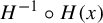
 , every endpoint of
$H^{-1}\circ H(x)$
 can be approached by points in
$\Gamma $
 . Combining (2.9) and (2.10), one just has (2.8).
For the third item, by Proposition 2.9,
$\bar {\Gamma }$
 is
$\mathcal {F}^{s/u}_F$
 -saturated. Let us consider
$f|_{\Lambda }$
 for the cases of
$sc$
 -DA and
$cu$
 -DA.
-
• In the $sc$
-DA case, it follows from Corollary 2.10 that f is special on the whole
$\mathbb {T}^2$
. In addition, the foliation
$\mathcal {F}^s_f$
exists and is the projection of
$\mathcal {F}^s_F$
. Hence,
$\Lambda $
is
$\mathcal {F}^s_f$
-saturated. -
• In the $cu$
-DA case, let
$x\in \Gamma $
and
$n\in \mathbb {Z}^2$
. Then, $$ \begin{align*} H( \mathcal{F}^u_F(x+n)-n ) &= H(\mathcal{F}^u_F(x+n))-n \\ &= \widetilde{\mathcal{L}}^u (H(x)+n)-n = \widetilde{\mathcal{L}}^u (H(x))=H(\mathcal{F}^u_F(x)). \end{align*} $$
Since $x\in \Gamma $
, one has
$\mathcal {F}^u_F(x+n)-n = \mathcal {F}^u_F(x)$
for any
$n\in \mathbb {Z}^2$
. By the continuity of
$\mathcal {F}^u_F$
,
$\mathcal {F}^u_F(z+n) = \mathcal {F}^u_F(z)+n$
for any
$z\in \bar \Gamma $
and
$n\in \mathbb {Z}^2$
. It follows that
$E^u_F(z+n)= DT_n(E^u(z))$
for any
$z\in \bar \Gamma $
and
$n\in \mathbb {Z}^2$
. Recall that
$T_n:\mathbb {R}^2\to \mathbb {R}^2$
is the deck transformation. Hence, $$ \begin{align*}T_{\Lambda}=E^c_f\oplus D\pi(E^u_F)\end{align*} $$is an invariant hyperbolic splitting, $f|_{\Lambda }$
is special, and
$\Lambda $
is
$\mathcal {F}^u_f$
-saturated.














For the fourth item, we just prove for
$\sigma =+$
 and
$\mathcal {F}^u_f$
 , since other cases are similar. Note that we do not know
$f|_{\mathbb {T}^2\setminus \Lambda }$
 is special yet, so it will be convenient to deal with this case in
$\mathbb {R}^2$
 . We equip the same orientation to
$\mathcal {F}^c_F$
 . Assume that there exist
$x=x^+\in \bar \Gamma $
 and
$y\in \mathcal {F}^u_F(x)$
 with
$y\neq y^+$
 . Then, one has
$y\prec y^+$
 . Let
$z = \mathcal {F}^u_F(y^+)\cap \mathcal {F}^c_F(x^+)$
 , one has
$x^+\prec z$
 by the holonomy map along unstable foliation. However,

which implies
$H(x^+)=H(z)$
 . It contradicts the choice of
$x^+$
 .
For the fifth item, let U be an open set with respect to the topology of
$\Lambda $
 . Then,
$h(U)$
 is an open set in
$\mathbb {T}^2$
 (see a precise proof in the next independent Lemma 2.12). It follows that there exists
$p'\in \mathrm {Per}(A)\cap h(U)$
 . Hence, the extreme point(s) of
$H^{-1}(p')$
 will be periodic in U.
To end this section, we give a further property of the semi-conjugacy h along center leaves, which can be regarded as a Cantor-like property.
Lemma 2.12. Let
$\Lambda $
 be given in Proposition 2.11, and h be the semi-conjugacy between f and A. Then, one has the following.
-
(1) For any $x\in \mathbb {T}^2$
and
$y\in \mathcal {F}^c_f(x)$
with
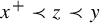
$x^+\prec y$
(or
$y \prec x^-$
), there exists
$z\in \mathcal {F}^c_f(x)$
such that
$h^{-1}\circ h(z)=\{z\}$
and
$x^+\prec z\prec y$
(or
$y\prec z\prec x^-$
). -
(2) Let $x\in \mathbb {T}^2$
and
$y_n\in \mathcal {F}^c_f(x)$
. If
$y_n\to x^{\sigma }$
as
$n\to +\infty $
, then
$y_n^\sigma \to x^\sigma $
, where
$\sigma =+$
or
$-$
. In particular, if
$y_n\prec x^-$
or
$x^+\prec y_n$
, then
$y_n^{-\sigma }\to x^\sigma $
as
$n\to +\infty $
. -
(3) For any $x\in \Lambda $
and
${\varepsilon }>0$
, the
${\varepsilon }$
-ball of x,
$B_{\varepsilon }(x)\subset \mathbb {T}^2$
satisfies that the set
${h(B_{\varepsilon }(x)\cap \Lambda )}$
has non-empty interior on
$\mathbb {T}^2$
.





Proof. The existence of center leaf
$\mathcal {F}^c_f(x)$
 for every
$x\in \mathbb {T}^2$
 is guaranteed by Corollary 2.10.
For the first item, let
$x=x^+$
 and
$y\in \mathcal {F}^c_f(x)$
 such that
$x^+\prec y$
 . By contradiction, we assume that for every
$z\in \mathcal {F}^c_f(x)$
 with
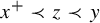
$x^+\prec z\prec y$
 , the set
$h^{-1}\circ h(z)$
 is a closed interval. From this assumption, two such adjacent intervals intersect with each other; hence, the union of these intervals is an interval that we denote by I. In particular, for every point
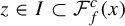
$z\in I\subset \mathcal {F}^c_f(x)$
 , one has
$h(z)=h(z_0)$
 , where
$z_0\in \mathcal {F}^c_f(x)$
 is a given point such that
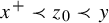
${x^+\prec z_0\prec y}$
 . Then, one can take
$z_n\in I$
 such that
$z_n\to x^+$
 with
$x^+\prec z_n$
 and
$h(z_n)=h(z_0)$
 . Since h is continuous,

It contradicts the fact that
$x^+\prec z$
 .
For the second item, we just prove the case of
$\sigma =+$
 and the other case is similar. Let
$x\in \mathbb {T}^2$
 and
$y_n\in \mathcal {F}^c_f(x)$
 with
$y_n\to x^+$
 . Taking a subsequence, one has
$x^+\prec y_n$
 or
$y_n\prec x^+$
 for all
$n\in \mathbb {N}$
 .
If
$x^+\prec y_n$
 for all
$n\in \mathbb {N}$
 , by the first item, there exists
$z_n\in \mathcal {F}^c_f(x)$
 such that
${x^+\prec z_n\prec y_n}$
 and
$h^{-1}\circ h(z_n)=\{z_n\}$
 . Here, one can assume that

Note that
$y_n \to x^+$
 , one has
$z_n\to x^+$
 . Hence,
$y_{n+1}^+\to x^+$
 and
$y_{n+1}^-\to x^+$
 as
$n\to +\infty $
 .
Let
$y_n\prec x^+$
 for all
$n\in \mathbb {N}$
 . If
$h^{-1}\circ h(x)$
 is an interval, then for large n, we have
${y_n\in h^{-1}\circ h(x)}$
 ; hence,
$y_n^+=x^+$
 . If
$h^{-1}\circ h(x)=\{x\}$
 , by the first item again, there exists
${z_n\in \mathcal {F}^c_f(x)}$
 such that

Hence, one can assume that

It follows from
$y_n\to x=x^+=x^-$
 that
$y^-_{n+1}\to x^+$
 and
$y^+_{n+1}\to x^+$
 as
$n\to +\infty $
 .
Finally, we prove the third item. Denote by
$\mathcal {L}^c$
 the foliation corresponding to
$H(\mathcal {F}^c_F)$
 on
$\mathbb {R}^2$
 . Note that H is homeomorphic along each leaf of the hyperbolic foliation
$\mathcal {F}^{s/u}_F$
 , and the center foliation
$\mathcal {F}^c_F$
 and hyperbolic one
$\mathcal {F}^{s/u}_F$
 admit the product structure. Hence, the third item follows from that for every
$x\in \Lambda $
 and
${\varepsilon }>0$
 , the
${\varepsilon }$
 -ball
$B_{\varepsilon }^c(x)$
 on center leaf
$\mathcal {F}^c_f(x)$
 satisfies that
$h(B_{\varepsilon }^c(x)\cap \Lambda )$
 has non-empty interior on
$\mathcal {L}^c(h(x))$
 .
Indeed, let
${\varepsilon }>0$
 and
$x=x^+$
 (or symmetrically
$x=x^-$
 ). By the second item, there exists
$y_n\in \mathcal {F}^c_f(x) \cap \Lambda $
 such that
$y_n=y_n^+\to x$
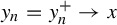 as
$n\to \infty $
 . In particular, there exists
${y_0=y_0^+\in B_{\varepsilon }^c(x)\cap \Lambda }$
 and
$x\prec y_0$
 . Since h is continuous and monotonic along the center leaf,
$h( [x,y_0] \cap \Lambda )=h( [x,y_0])$
 is an interval contained in
$h(B_{\varepsilon }^c(x)\cap \Lambda )$
 .
3 The special property implies semi-conjugacy
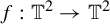
In this section, we will prove Theorem A. Let
$f:\mathbb {T}^2\to \mathbb {T}^2$
 be a
$C^1$
 -smooth special DA endomorphism with the hyperbolic linearization
$A:\mathbb {T}^2\to \mathbb {T}^2$
 . We will show that the existence of a
$Df$
 -invariant dominated splitting into direct sum of subbundles implies the existence of a semi-conjugacy. The property holds for both
$sc$
 -DA and
$cu$
 -DA cases, but their proofs have some differences. We would like to present some common lemmas and prove for these two cases independently. Specifically, Theorem A will follow from Corollaries 3.5 and 3.7.
Since f is special, the foliations
$\mathcal {F}^1$
 and
$\mathcal {F}^2$
 given in Proposition 2.7 are now
$\mathbb {Z}^2$
 -periodic, that is,
$\mathcal {F}^i(x+n)=\mathcal {F}^i(x)+n$
 for any
$x\in \mathbb {R}^2$
 ,
$n\in \mathbb {Z}^2$
 , and
$i=1,2$
 . Let
$H:\mathbb {R}^2\to \mathbb {R}^2$
 be the semi-conjugacy between the lifted maps
$F:\mathbb {R}^2\to \mathbb {R}^2$
 and
${A:\mathbb {R}^2\to \mathbb {R}^2}$
 .
Fix
$x_0\in \mathbb {R}^2$
 , so the map

given by
$H_n(x)=H(x-n)+n$
 is well defined. In particular, let
$x_0\in \mathbb {R}^2$
 be a fixed point of F. Note that Fix
$(F)\neq \emptyset $
 . Indeed, let
$0\in \mathbb {R}^2$
 be the unique fixed point of A. By Proposition 2.9,
$H^{-1}(0)$
 is either a single point (hence, a fixed point of F), or a compact local center leaf that admits at least one fixed point.
Moreover, we consider the following map:

given by
$\overline {H}(x)=H_{n_x}(x)$
 for any
$x\in \mathcal {F}^2(x_0+n_x)$
 .
Lemma 3.1. If
$\mathcal {F}^2(x_0+n)=\mathcal {F}^2(x_0+m)$
 for some
$n\neq m\in \mathbb {Z}^2$
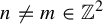 , then
$H_n=H_m$
 .
Remark 3.2. We can see
$x_0+n\notin \mathcal {F}^2(x_0)$
 for any
$n\in \mathbb {Z}^2$
 , so we can actually define
$\overline {H}$
 without Lemma 3.1. Indeed, if f is
$cu$
 -DA, then
$\mathcal {F}^2(x_0)$
 is a one-dimensional unstable manifold, so it cannot be a circle. When f is
$sc$
 -DA, if there is an
$n_0\in \mathbb {Z}^2$
 such that
$x_0+n_0\in \mathcal {F}^2(x_0)$
 , then the one-dimensional leaf
$\mathcal {F}^2(x_0)$
 module
$\mathbb {Z}^2$
 cannot be dense in a fundamental domain, which contradicts Proposition 3.4. However, Lemma 3.1 can be of independent interest as it can be generalized for higher-dimensional
$\mathcal {F}^2$
 (based on the argument of the proof without restriction on the dimension).
Proof of Lemma 3.1.
Let
$x\in \mathcal {F}^2(x_0+n)=\mathcal {F}^2(x_0+m)$
 . By Proposition 2.6,

However,
$x_0+m-n\in \mathcal {F}^2(x_0)$
 since f is special and
$x_0+m\in \mathcal {F}^2(x_0+m)= \mathcal {F}^2(x_0+n)$
 . We claim that

Otherwise, if
$H(x_0)+m-n\notin \widetilde {\mathcal {L}}^u(H(x_0))$
 , one will get two contradictory facts:
-
• $d(H(x_0)+k(m-n),\ \widetilde {\mathcal {L}}^u (H(x_0)) )\to +\infty $
, as
$k\to +\infty $
; -
• since f is special, for every $k\in \mathbb {N}$
, one has
$x_0+k(m-n)\in \mathcal {F}^2(x_0)$
. Moreover, by
$\|H-\mathrm {Id}_{\mathbb {R}^2}\|_{C^0}<C_H$
(Proposition 2.5), one can get $$ \begin{align*} H(x_0)+k(m-n) &\in B_{2C_H}( H(x_0+k(m-n)))\\ &\subset B_{2C_H}(H(\mathcal{F}^2(x_0))) = B_{2C_H}(\widetilde{\mathcal{L}}^u(H(x_0))). \end{align*} $$






By (3.2), it follows that

This implies
$\widetilde {\mathcal {L}}^u(H(x_0)+m)=\widetilde {\mathcal {L}}^u(H(x_0)+n)$
 . Thus, combining with (3.1) and the global product structure, one has
$H_n(x)=H_m(x)$
 .
For short, we denote the domain of the map
$\overline {H}$
 by

We are going to prove that the map
$\overline {H}$
 is equal to H on a large set, see also [Reference Moosavi and Tajbakhsh43] for this method to deal with special Anosov endomorphisms on nilmanifolds. We mention in advance that when f is
$sc$
 -DA,
$\bar {\mathbf {F}}=\mathbb {R}^2$
 and
$\overline {H}$
 can be extended to
$\mathbb {R}^2$
 . However, when f is
$cu$
 -DA, we have no a priori
$\bar {\mathbf {F}}=\mathbb {R}^2$
 and this will be an obstacle.
Lemma 3.3. The map
$\overline {H}$
 (defined on
$\mathbf {F}$
 ) satisfies:
-
(1) $\overline {H}\circ F= A\circ \overline {H}$
; -
(2) there exists $C_{\overline {H}}>0$
such that
$\| \overline {H}-\mathrm {Id}_{\mathbf {F}} \|_{C^0}<C_{\overline {H}}$
; -
(3) $\overline {H}$
is uniformly continuous; -
(4) $\overline {H}(x+n)= \overline {H}(x)+n$
for any
$x\in \mathbf {F}$
and
$n\in \mathbb {Z}^2$
.







Proof. For the first item, let
$x\in \mathbf {F}$
 . There exists
$n_x\in \mathbb {Z}^2$
 with
$x\in \mathcal {F}^2(x_0+n_x)$
 . Since
$x_0\in \mathrm {Fix}(F)$
 ,

and

The second item follows from the corresponding facts of the map H by taking
$C_{\overline {H}}=C_H$
 . Now, we continue to prove the third item.
By the definition and the uniform continuity of H on
$\mathbb {R}^2$
 ,
$\overline {H}$
 is uniformly continuous along each leaf of
$\mathcal {F}^2$
 , namely, for given
${\varepsilon }>0$
 , there exists
$\delta>0$
 such that for any
$n\in \mathbb {Z}^2$
 and any
$x,y\in \mathcal {F}^2(x_0+n)$
 with
$d(x,y)<\delta $
 , then
$d(\overline {H}(x),\overline {H}(y))<{\varepsilon }$
 . From the global product structure, and the uniform angle between bundles
$E^1$
 and
$E^2$
 , the proof remains to show the uniform continuity along
$\mathcal {F}^1$
 , the transverse foliation of
$\mathcal {F}^2$
 .
By contradiction, we assume that there exists
${\varepsilon }_0$
 such that for any
$\delta _k> 0$
 , there are two points

for some
$n_k, m_k\in \mathbb {Z}^2$
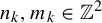 , such that
$d(x_k,y_k)<\delta _k$
 and
$d(\overline {H}(x_k),\overline {H}(y_k))\geqslant {\varepsilon }_0$
 .
Note that
$\overline {H}(y_k)\in \widetilde {\mathcal {L}}^s(\overline {H}(x_k))$
 . Indeed, by Proposition 2.9, one has

Since
$d(\overline {H}(x_k),\overline {H}(y_k))\geqslant {\varepsilon }_0$
 with

by the global product structure of
$\widetilde {\mathcal {L}}^s$
 and
$\widetilde {\mathcal {L}}^u$
 , these two parallel lines in
$\mathbb {R}^2$
 ,

satisfy that there is
$\eta _0>0$
 relying only on
${\varepsilon }_0$
 and A such that

Moreover, for any
$l\in \mathbb {N}$
 ,

However, since
$d(x_k,y_k)<\delta _k$
 , one has

equivalently,

In particular, for any
$l\in \mathbb {N}$
 ,

which implies

Since
$\|H-\mathrm {Id}_{\mathbb {R}^2}\|_{C^0}<C_H$
 , one has
$d(\mathcal {F}^2(x_0) ,\ \widetilde {\mathcal {L}}^u(H(x_0))) <C_H$
 . Combining with (3.4), one has

For a given
$\eta _0$
 , one can choose
$l\in \mathbb {N}$
 such that
$l\eta _0>3C_H$
 . Moreover, let
$\delta _k$
 be small enough such that
$l\delta _k<C_H$
 . Then, (3.5) contradicts (3.3).
Finally, we prove the fourth item. Since
$\mathcal {F}^2$
 is
$\mathbb {Z}^2$
 -periodic, for any
$n\in \mathbb {Z}^2$
 , one has

On the one hand, by the definition of
$\overline {H}$
 , one has

where the last equality comes from
$\overline {H}(x)\in \widetilde {\mathcal {L}}^u( H(x_0)+n_x)$
 . On the other hand, according to Proposition 2.6 (without the assumption that f is special and
$x\in \mathbf {F}$
 ) and
$x+n\in \mathcal {F}^2(x_0+n_x+n)$
 ,

where the first inclusion and the last equality are exactly based on Proposition 2.6. Thus,

which implies
$\overline {H}(x+n)= \overline {H}(x)+n$
 .
Now, we split the proof of Theorem A as the following two cases.
Proposition 3.4. Under the assumption of Theorem A, if f is
$sc$
 -DA, then

Proof. Here, f is
$sc$
 -DA,
$\mathcal {F}^2(x_0+n)=\mathcal {F}^c_F(x_0+n)$
 , and

By Proposition 2.2, one has

is dense in
$\mathbb {R}^2$
 . In addition, according to Proposition 2.6, one has
$n^*\in A^k\mathbb {Z}^2$
 such that
$\widetilde {\mathcal {L}}^u(H(x_0)+n^*)$
 and
$\widetilde {\mathcal {L}}^u(H(x_0+n^*))$
 are close, so one can get

Thus, by Proposition 2.9, H is a homeomorphism restricted to
$\mathcal {F}_F^s$
 and the conclusion follows.
There is a direct corollary of Proposition 3.4 and the fourth item of Lemma 3.3.
Corollary 3.5. Under the assumption of Theorem A, if f is
$sc$
 -DA, then
$\overline {H}$
 can uniquely continuously extend to be H. Moreover,
$H(x+n)=H(x)+n$
 for any
$x\in \mathbb {R}^2$
 and
$n\in \mathbb {Z}^2$
 . In particular,
$h:=\pi \circ H\circ \pi ^{-1}$
 is well defined on
$\mathbb {T}^2$
 and a semi-conjugacy between f and A.
Now, we deal with the case of
$cu$
 -DA. Recall that
$\bar {\Gamma }$
 , the closure of the H-injective set,

is an F-invariant set.
Proposition 3.6. Under the assumption of Theorem A, if f is
$cu$
 -DA, then:
-
(1) $\bar {\Gamma } \subset \bar {\mathbf {F}}$
, the closure of set
$\mathbf {F}$
; -
(2) $\overline {H}$
uniquely continuously extends to
$\bar {\Gamma }$
such that
$\overline {H}|_{\bar {\Gamma }}=H|_{\bar {\Gamma }}$
and
$H(\bar {\Gamma })=\mathbb {R}^2$
; -
(3) $H(x+n)=H(x)+n$
for any
$x\in \bar {\Gamma }$
and
$ n\in \mathbb {Z}^2$
; -
(4) $\bar {\Gamma }+\mathbb {Z}^2=\bar {\Gamma }$
.





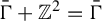
Proof. To prove the first item, applying the same method as in the proof of Proposition 3.4, one has

is dense in
$\mathbb {R}^2$
 , by Propositions 2.2 and 2.6. Note that it does not imply
$\bar {\mathbf {F}}=\mathbb {R}^2$
 since H may not be homeomorphic along
$\mathcal {F}^1$
 in this case. However,
$\mathbf {F}$
 is dense in
$\bar {\Gamma }$
 . Indeed, let
$x\in \bar {\Gamma }$
 . Since
$H|_{\mathcal {F}_F^c(x)}$
 is not locally constant at x, for every short open segment
$J^c$
 containing x on
$\mathcal {F}^c_F(x)$
 , there exists a non-trivial closed interval
$I^c\subset J^c$
 such that
$H(I^c)$
 has positive length and
$H^{-1}\circ H(I^c)=I^c$
 . Since
$H(\mathbf {{F}})$
 is dense in
$\mathbb {R}^2$
 , there exists
$n^*\in \mathbb {N}$
 such that the leaf

intersects with
$H(I^c)$
 at a point z. Thus, the set
$H^{-1}(z)\subset I^c\subset J^c$
 and the leaf
${\mathcal {F}_F^u(x_0+n^*)}$
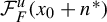 intersects
$J^c$
 . This implies
$\bar {\Gamma } \subset \bar {\mathbf {F}}$
 .
Recall that by Proposition 2.9,
$\bar {\Gamma }= \bigcup _{x\in \mathbb {R}^2} \{ y\in \mathbb {R}^2\mid y\ \text {is an endpoint of} \ H^{-1}\circ H(x)\}$
 . Thus,
$H(\bar {\Gamma })=\mathbb {R}^2$
 . The second item follows from the uniqueness of H in Proposition 2.5 and the fact that
$\bar \Gamma $
 is
$F^{\pm 1}$
 -invariant. Indeed, for every
$x\in \bar \Gamma $
 and
$k\in \mathbb {Z}$
 ,

where
$\|H-\mathrm {Id}_{\mathbb {R}^2}\|_{C^0}\leqslant C_H$
 and
$\|\overline {H}-\mathrm {Id}_{\bar \Gamma }\|_{C^0}\leqslant C_{\overline {H}}=C_H$
 . By (3.6),
$H(x)=\overline {H}(x)$
 for all
$x\in \bar \Gamma $
 .
The third item is a corollary of the first two items. By the fourth item of Lemma 3.3, for any
$x\in \bar {\Gamma }$
 and
$n\in \mathbb {Z}^2$
 , one has that
$x+n\in \bar {\Gamma }+\mathbb {Z}^2\subset \bar {\mathbf {F}}$
 ; hence,
$\overline {H}(x+n)= \overline {H}(x)+n=H(x)+n$
 . However, we do not know a priori that
$x+n\in \bar {\Gamma }$
 nor that
$\overline {H}(x+n)=H(x+n)$
 . To prove this, it suffices to show that
$\bar {\mathbf {F}}$
 is an F-invariant set. Then, by the same argument of the second item, one has that
$\overline {H}|_{\bar {\mathbf {F}}}=H|_{\bar {\mathbf {F}}}$
 ; hence,
$\overline {H}(x+n)=H(x+n)$
 .
Now, we prove the F-invariance of
$\bar {\mathbf {F}}$
 , which is in fact a corollary of the first item. Note that there exist
$n_i\in \mathbb {Z}^2 \ (1\leqslant i\leqslant l=\mathrm {deg}(A))$
 such that
$\mathbb {Z}^2= \bigcup _{1\leqslant i\leqslant l}(n_i+A\mathbb {Z}^2)$
 and

By the proof of the first item,
$\bar {\Gamma }\subset \overline {\mathcal {F}^u_F(x_0+n_i)+A\mathbb {Z}^2}$
 for every
$1\leqslant i\leqslant l$
 . Hence, we can take

It follows that there are
$m^1_j\in A\mathbb {Z}^2$
 and
$m^2_j\in A\mathbb {Z}^2$
 such that when
$j\to +\infty $
 ,

Therefore,
$\mathcal {F}^u_F(x_0)+m^1_j-m^2_j \to \mathcal {F}^u_F(x_0+n_i)$
 as
$j\to +\infty $
 . Note that
$(m^1_j-m^2_j)\in A\mathbb {Z}^2$
 , so

It follows from (3.7) and (3.8) that
$F(\bar {\mathbf {F}})=\overline {\mathcal {F}^u_F(x_0)+A\mathbb {Z}^2}=\bar {\mathbf {F}}$
 .
For the fourth item, we first claim that for any
$z\in \Gamma $
 and
$n\in \mathbb {Z}^2$
 , we have
$z+n\in \bar {\Gamma }$
 . Indeed, if there exist
$z_0\in \Gamma $
 and
$n_0\in \mathbb {Z}^2$
 such that
$z_0+n_0\notin \bar {\Gamma }$
 , we can take
$y\in \partial \bar {\Gamma }\subset \bar {\Gamma }$
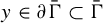 with
$y\neq z_0+n_0$
 such that
$H(y)=H(z_0+n_0)$
 . By the third item,

By the injection of H on
$\Gamma $
 , it follows that
$y-n_0=z_0$
 , which is an obvious contradiction. Then, for any
$x\in \bar {\Gamma }$
 and
$n\in \mathbb {Z}^2$
 , there exists
$z_k\in \Gamma $
 such that
$z_k\to x$
 . Note that
${z_k+n \in \bar {\Gamma }}$
 , one has
$z_k+n\to x+n\in \bar {\Gamma }$
 .
Corollary 3.7. Under the assumption of Theorem A, if f is
$cu$
 -DA, then
$H(x+n)=H(x)+n$
 for any
$x\in \mathbb {R}^2$
 and
$ n\in \mathbb {Z}^2$
 . In particular,
$h:=\pi \circ H\circ \pi ^{-1}$
 is well defined on
$\mathbb {T}^2$
 , and a semi-conjugacy between f and A.
Proof. By the third item of Proposition 3.6, we need only show
$H(x+n)=H(x)+n$
 for
$x\in \bar {\Gamma }^c$
 , the complement of
$\bar {\Gamma }$
 . By Proposition 2.9, there exists
$y\in \bar {\Gamma }$
 such that the curve
$[x,y)\subset \mathcal {F}_F^c(x)\cap \bar {\Gamma }^c$
 and
$H(x)=H(y)$
 . Then, by the fourth item of Proposition 3.6, one has that
$y+n\in \bar {\Gamma }$
 and

for any
$n\in \mathbb {Z}^2$
 . Hence,
$H(x+n)=H(y+n)=H(y)+n=H(x)+n$
 .
4 Rigidity of Lyapunov exponents
Let
$f:\mathbb {T}^2\to \mathbb {T}^2$
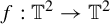 be a
$C^1$
 -smooth DA endomorphism and
$A:\mathbb {T}^2\to \mathbb {T}^2$
 be its linearization. Let f be semi-conjugate to
$A:\mathbb {T}^2\to \mathbb {T}^2$
 and
$\Lambda $
 be given in Proposition 2.11. Note that
$\Lambda $
 is
$\mathcal {F}^{s/u}_f$
 -saturated and
$f|_{\Lambda }$
 is special. Also, f has uniquely integrable center bundle (Corollary 2.10).
For
$\{x_n\}\subset \Lambda $
 ,
$x\in \Lambda $
 , and
$\sigma =+\ \mathrm {or}\ -$
 , we define
$x_n\to _\sigma x$
 (see Figure 2) as
$x_n$
 converging to x along the
$\sigma $
 -direction of the center foliation
$\mathcal {F}^c_f$
 . Precisely, by the local product structure, let
$x^{\prime }_n$
 be the unique intersection of local leaves
$\mathcal {F}^c_f(x)$
 and
$\mathcal {F}^{s/u}_f(x_n)$
 . Since
$\Lambda $
 is
$\mathcal {F}^{s/u}_f$
 -saturated, we have
$x^{\prime }_n\in \Lambda $
 . Then, we can define the following.
-
• We say $x_n\to _+ x$
if
$x\prec x^{\prime }_n$
and
$d(x_n,x)\to 0$
as
$n\to +\infty $
. -
• We say $x_n\to _- x$
if
$x^{\prime }_n\prec x$
and
$d(x_n,x)\to 0$
as
$n\to +\infty $
.







The definition of
$x_n\to _{\pm }x$
 . (Color online.)

Figure 2 Long description
The diagram consists of two panels showing the relationship between center foliations and stable or unstable foliations.
Left Panel:
- A horizontal blue line is labeled script F sub f super c of x. It has a minus sign on the left and a plus sign on the right.
- Three vertical red curves, labeled script F sub f super s forward slash u, intersect the blue line.
- On the leftmost red curve, the intersection point is a black dot labeled x.
- On the middle red curve, there is a black dot labeled x sub n plus 1 above the blue line, and an x-mark labeled x prime sub n plus 1 at the intersection with the blue line.
- On the rightmost red curve, there is a black dot labeled x sub n above the blue line, and an x-mark labeled x prime sub n at the intersection with the blue line.
- Below the panel, text reads x sub n approaches sub plus x.
Right Panel:
- A horizontal blue line is labeled script F sub f super c of x with a minus sign on the left and a plus sign on the right.
- Three vertical red curves, labeled script F sub f super s forward slash u, intersect the blue line.
- On the leftmost red curve, there is a black dot labeled x sub n above the blue line, and an x-mark labeled x prime sub n at the intersection with the blue line.
- On the middle red curve, there is a black dot labeled x sub n plus 1 above the blue line, and an x-mark labeled x prime sub n plus 1 at the intersection with the blue line.
- On the rightmost red curve, the intersection point is a black dot labeled x.
- Below the panel, text reads x sub n approaches sub minus x.
Similarly, we can define

as
$x_n$
 converging to x along the
$\sigma $
 -direction of the corresponding foliation
$\mathcal {L}^c:=h(\mathcal {F}^c_f)$
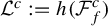 . In addition, we assume that h preserves the orientation on each leaf.
Let
$F:\mathbb {R}^2\to \mathbb {R}^2$
 be a lift of f via
$\pi :\mathbb {R}^2\to \mathbb {T}^2$
 and admit the invariant partially hyperbolic splitting given as (2.6),

Denote by
$\unicode{x3bb} ^1(p)$
 the Lyapunov exponent of point
$p\in \mathbb {T}^2$
 with respect to the bundle

Recall that
$E^1$
 is uniquely integrable and so is
$E_1$
 (Proposition 2.7). We denote the integral foliation by
$\mathcal {F}_1$
 , and denote the infimum and supremum of the set

by
$\unicode{x3bb} _-$
 and
$\unicode{x3bb} _+$
 , respectively.
We mainly obtain the following rigidity result for DA endomorphisms on
$\mathbb {T}^2$
 .
Proposition 4.1. Let
$f:\mathbb {T}^2\to \mathbb {T}^2$
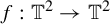 be a
$C^1$
 -smooth DA endomorphism semi-conjugate to its hyperbolic linearization
$A:\mathbb {T}^2\to \mathbb {T}^2$
 . Let
$\Lambda $
 be given in Proposition 2.11. If
$\unicode{x3bb} _-<0$
 , then
$\unicode{x3bb} ^1(p)=\unicode{x3bb} ^1(q)$
 for any
$p,q\in \mathrm {Per}(f|_{\Lambda })$
 .
Before giving the proof of Proposition 4.1, we first give an adapted metric with respect to the periodic data on the set
$\Lambda $
 . Recall that
$\Lambda $
 is exactly the collection of the endpoints of
$h^{-1}\circ h(x)$
 for all
$x\in \mathbb {T}^2$
 .
Proposition 4.2. Let
$f:\mathbb {T}^2\to \mathbb {T}^2$
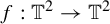 be a
$C^1$
 -smooth DA endomorphism semi-conjugate to its hyperbolic linearization
$A:\mathbb {T}^2\to \mathbb {T}^2$
 . Let
$\Lambda $
 be given in Proposition 2.11. Then, for any
$\delta>0$
 , there exists a Riemannian metric
$\|\cdot \|$
 such that for every
$x\in \Lambda $
 ,

Proof. The existence of an adapted metric we desired follows from Lemma 4.3, which can be viewed as a non-uniformly shadowing property.
Lemma 4.3. Let
$\mu $
 be an ergodic measure with
$\mathrm {supp}(\mu )\subset \Lambda $
 . Then,
$\mu $
 can be approached by periodic measures supported on
$\Lambda $
 with respect to the weak-star topology. In particular, there exists a sequence of periodic points
$p_n\in \Lambda $
 such that

In particular,
$\unicode{x3bb} _-\leqslant \unicode{x3bb} ^1(\mu )\leqslant \unicode{x3bb} _+$
 .
Proof of Lemma 4.3.
We just prove in the case of
$sc$
 -DA, as the other case is quite similar.
For a given ergodic measure
$\mu $
 supported on
$\Lambda $
 , by the Poincaré recurrence theorem, we can take a recurrent
$\mu $
 -typical point x. Since
$\mu $
 is supported on
$\Lambda $
 ,
$x\in \Lambda $
 . Then, we can assume that
$x=x^+$
 . In addition, the case of
$x=x^-$
 follows the similar argument. For convenience, we assume that f preserves the orientation on center leaves.
For a given negative f-orbit
$x_{-n},\ldots ,x_{-1},x$
 of x, we have
$x_{-i}=x^+_{-i}$
 for any
$1\leqslant i\leqslant n$
 . To simplify, we still denote by
$\mathcal {F}^c_f(x,{\varepsilon })$
 the positive-orientation component of the local center leaf of
$x^+$
 , namely,
$y\in \mathcal {F}^c_f(x,{\varepsilon })$
 implies
$y\in \mathcal {F}^c_f(x)$
 with
$d_{\mathcal {F}^c_f}(x,y)\leqslant {\varepsilon }$
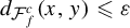 and
$x\prec y$
 . In addition, we denote the component of
$f^{-i}(\mathcal {F}^c_f(x,{\varepsilon }))$
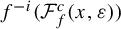 containing
$x_{-i}$
 by
$f_0^{-i}(\mathcal {F}^c_f(x,{\varepsilon }))$
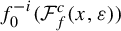 for any
$0\leqslant i\leqslant n$
 .
We first claim that the local center leaf of x has topological contraction (see also [Reference Pujals and Sambarino51]) property along the negative orbit.
Claim 4.4. Given
$x=x^+\in \Lambda $
 . For any given
${\varepsilon }>0$
 , there exists
$\eta>0$
 such that for every negative f-orbit
$x_{-n},\ldots ,x_{-1},x$
 of x, one has

Proof of Claim 4.4.
By contradiction, we assume that there exists
${\varepsilon }_0>0$
 such that for any
$\eta _m>0$
 , there exists an f-orbit
$x_{-n_m},\ldots ,x_{-1},x$
 such that the lengths of local leaves

and

where C only depends on f. Note that we can take
$\eta _m\to 0$
 ; hence,
$n_m\to +\infty $
 .
Let
$I_m:=f^{-n_m}_0(\mathcal {F}^c_f(x,\eta _m))$
 . By the compactness of
$\Lambda $
 and the continuity of
$\mathcal {F}_f^c$
 , we can assume that
$x_{-n_m}\to z\in \Lambda $
 and
$I_m\to I\subset \mathcal {F}^c_f(z)$
 with length
${\varepsilon }_0\leqslant |I| \leqslant C{\varepsilon }_0$
 . Moreover,
$|f^n(I)|\leqslant C{\varepsilon }_0$
 for any
$n\in \mathbb {N}$
 . Indeed, for given
$n\geqslant 1$
 , by (4.1), when m is big enough,
$|f^n(I_m)|\leqslant {\varepsilon }_0$
 and
$f^n(I_m)\to f^n(I)$
 as
$m\to +\infty $
 . Hence, by the uniform continuity of h, there exists a constant
$L_0>0$
 such that

However, note that
$x_{-n_m}=x^+_{-n_m}$
 , we get
$z=z^+$
 and every
$y\in I$
 satisfies
$z\prec y$
 , then we have
$|h(I)|>0$
 . Thus, by
$h(I)\subset \mathcal {L}^u(h(z))$
 , we further have

From the topological contraction property, we prove Lemma 4.3 as follows.
Note that for
$x=x^+$
 , we can assume there exists a preimage sequence
$x_{-n_k}\to _+ x$
 . Indeed, let
$\bar {x}=h(x)$
 . Applying Lemma 2.3 for choosing A-preimages of
$\bar {x}$
 in small balls that are close to
$\bar {x}$
 in its positive direction (with respect to the orientation of
$h(\mathcal {F}^c_f)$
 ), one has

where
$A^{n_k}(\bar {x}_{-n_k})=\bar {x}$
 . Let
$x_{-n_k}=x_{-n_k}^+$
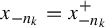 be the positive boundary of
$h^{-1}(\bar {x}_{-n_k})$
 . Then, one has
$f^{n_k}(x_{-n_k})=x$
 and by Lemma 2.12, one can get

For a recurrence point
$x_{-n_k}$
 and its related pseudo periodic f-orbit

the corresponding sequence

gives a pseudo-periodic A-orbit. By the shadowing property of Anosov endomorphisms (see [Reference Aoki and Hiraide2]), for any
${\varepsilon }>0$
 , there exist
$x_{-n_k}$
 and a periodic point
$p^{\prime }_k$
 of A with
$A^{n_k}(p_k')=p_k'$
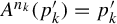 such that

Moreover, when
$x_{-n_k}\to _+ x$
 , one has
$h(x_{-n_k})\to ^A_+ h(x)$
 and
$p_k'\to ^A_+ h(x)$
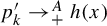 .
The shadowing property on the set
$\Lambda $
 . (Color online.)

Figure 3 Long description
The diagram consists of three panels connected by horizontal arrows pointing right.
Panel 1 (Left): A dashed circle labeled B (x sub minus i, epsilon) contains a grid formed by two vertical red curves labeled script F sub f super s and two horizontal blue curves labeled script F sub f super c. Four intersection points are marked: x sub minus i (top-left), z sub k super minus i (top-right), w sub k super minus i (bottom-left), and p sub k super minus i (bottom-right). An arrow labeled f super i points to the second panel.
Panel 2 (Center): A similar dashed circle labeled B (x, epsilon). The grid of red and blue curves persists. The intersection points are now labeled x = x super plus (top-left), z sub k (top-right), w sub k (bottom-left), and p sub k = p sub k super minus (bottom-right). A small ‘x’ mark labeled x sub minus n sub k is located in the upper right quadrant of the circle. An arrow labeled h points to the third panel.
Panel 3 (Right): A Cartesian coordinate system. The vertical axis is labeled script L super s and the horizontal axis is labeled script L super u. The origin is a black dot labeled h(x). To the right of the vertical axis is a dashed vertical line. On this dashed line, an ‘x’ mark is labeled h(x sub minus n sub k). To the right of the dashed line and below the horizontal axis is a black dot labeled p prime sub k.
Let
$p_k=p^-_k\in \Lambda $
 be the negative endpoint of
$h^{-1}(p_k')$
 . Then, one has
$f^{n_k}(p_k)=p_k.$
 By Lemma 2.12, for any
${\varepsilon }>0$
 , when
$x_{-n_k}$
 is sufficiently close to x, one can get
$p_k\to _+ x$
 with
$d(p_k,x)<{\varepsilon }$
 . Let
$z_k$
 be the unique intersection point of local leaves
$\mathcal {F}^s_f(p_k)$
 and
$\mathcal {F}^c_f(x)$
 , and
$w_k$
 be the unique intersection point of local leaves
$\mathcal {F}^c_f(p_k)$
 and
$\mathcal {F}^s_f(x)$
 . For
$1\leqslant i\leqslant n_k$
 , we denote the components of
$f^{-i}(z_k)$
 and
$f^{-i}(w_k)$
 on local leaves of
$x_{-i}$
 by
$z_k^{-i}$
 and
$w_k^{-i}$
 , respectively. Similarly, we denote by
$p_k^{-i}$
 the component of
$f^{-i}(p_k)$
 on a local leaf
$\mathcal {F}^s_f(z_k^{-i})$
 . See Figure 3. Note that h restricted to stable leaves is homeomorphic. Hence, for given
${\varepsilon }>0$
 , there exist
$x_{-n_k}$
 and
$p_k'$
 satisfying

However, for given
${\varepsilon }>0$
 , let
$\eta>0$
 be given in Claim 4.4. When
$x_{-n_k}$
 is sufficiently close to x, one has
$z_k\in \mathcal {F}^c_f(x,\eta )$
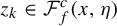 ; hence,

As a result, by choosing
$x_{-n_k}$
 appropriately, one can get
$d(p^{-i}_k,x_{-i})<{\varepsilon }$
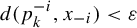 for all
${0\leqslant i\leqslant n_k}$
 .
Moreover, note that x is
$\mu $
 -typical, so the ergodic measure
$\mu $
 has the following form:

thus, it can be approached by periodic measures

where
$\delta _y$
 is a Dirac measure of the point y. Hence, the sequence of periodic points
$p_k\in \Lambda $
 satisfies

This ends the proof of Lemma 4.3.
Now, we prove the existence of the adapted metric
$\|~\|$
 . Let
$\delta>0$
 and
$|\cdot |$
 be a Riemannian metric given in advance. Note that for every point
$x\in \Lambda $
 , there exists a subsequence of the measures
$\{\mu _{x,n}\}_{n\in \mathbb {N}}$
 converging to an invariant measure
$\mu $
 with
$\mathrm {supp}(\mu )\subset \Lambda $
 , where

For short, let
$\mu _{x,n}\to \mu $
 . It follows from Lemma 4.3 and the ergodic decomposition that

Thus, there exists
$N=N(x,\delta )\in \mathbb {N}$
 such that for every
$n\geqslant N$
 ,

Note that f is
$C^1$
 and the bundle
$E_1$
 is continuous, by fixing
$n\geqslant N$
 , there exists an open neighborhood
$U=U(x,n)\subset \Lambda $
 of x such that for every
$y\in U$
 ,

By the compactness of
$\Lambda $
 , there exist finite points
$x_1,\ldots , x_m\in \Lambda $
 , finite times
${n_i\in \mathbb {N}\ (1\leqslant i\leqslant m)}$
 and finite neighborhoods
$U_i=U(x_i,n_i)\subset \Lambda \ (1\leqslant i\leqslant m)$
 such that
$\bigcup _{i=1}^m U_i=\Lambda $
 and

for every
$y\in U_i$
 . Let

for every
$v\in E_1(x)$
 and every
$x\in \Lambda $
 . Note that the norm
$\|\cdot \|_i$
 of the one-dimensional bundle
$E_1$
 actually induces a norm on
$T \Lambda $
 (see [Reference Bochi, Katok and Rodriguez Hertz4, (3.6)]) and

Hence, for every
$x\in U_i$
 , one has

Let
$\{ \phi _i\}_{i=1}^m$
 be a unit decomposition subordinated to
$\{ U_i\}_{i=1}^m$
 , namely,
$\phi _i$
 is
$C^{\infty }$
 , and supported on
$U_i$
 and
$\sum _{i=1}^m\phi _i=1$
 . For every
$x\in \Lambda $
 and
$v\in E_1(x)$
 , let

Then,
$\|\cdot \|$
 induces the metric we desired. This ends the proof of Proposition 4.2.
With the help of the adapted metric
$\|\cdot \|$
 , we prove the rigidity of DA endomorphisms now.
Proof of Proposition 4.1.
By contradiction, we assume that there exist
$p_0,q_0\in \mathrm {Per}(f|_{\Lambda })$
 such that
$\unicode{x3bb} ^1(p_0)<\unicode{x3bb} ^1(q_0)$
 . Then, we have

Given
$\delta>0$
 arbitrarily small, we can choose two periodic points
$p,q\in \mathrm {Per}(f|_{\Lambda })$
 such that

Moreover, by Proposition 4.2, we can assume that
$\|\cdot \|$
 is the norm with

since Lyapunov exponents of a regular point are independent of the choice of equivalent metrics. Furthermore, by the uniform continuity, we can also take
$\eta _0>0$
 such that for any
$x,y\in \mathbb {T}^2$
 with
$d(x,y)\leqslant \eta _0$
 , it follows that

Here, we fix the positive constant
$\delta $
 with

where

as in Claim 4.8.
For convenience, we can assume that both p and q are fixed points. Otherwise, we can apply the following proof to
$f^{n_0}$
 , with
$n_0$
 being a common period of p and q. We further assume that
$p=p^+$
 and consider two different cases:
$q=q^+$
 and
$q=q^-$
 . Here, we mention in advance that the
$sc$
 -DA case and
$cu$
 -DA case have some differences and similarities. In particular, the following claims (Claims 4.5, 4.6, 4.7, and 4.8) exhibit the same dynamical properties for both the
$sc$
 -DA case and
$cu$
 -DA case, but their proofs are somewhat different.
Let
$H:\mathbb {R}^2\to \mathbb {R}^2$
 be the semi-conjugacy between F and A given in Proposition 2.5. Then, we denote by
$h=\pi \circ H\circ \pi ^{-1}:\mathbb {T}^2\to \mathbb {T}^2$
 the semi-conjugacy between f and A. For
$x\in \Lambda $
 , we can assume that h restricted to leaves
$\mathcal {F}_1(x)$
 and
$\mathcal {F}_2(x)$
 preserves the orientation, respectively.
Claim 4.5. Given two points
$x=x^\sigma , y=y^\sigma \in \Lambda \ (\sigma =+ \ \mathrm {or}\ -)$
 , then for any
${{\varepsilon }>0}$
 , there exist
$k_{\varepsilon }=k({\varepsilon },x,y) \in \mathbb {N}$
 and
$x_{\varepsilon }=x_{\varepsilon }^\sigma \in \Lambda $
 such that
$f^{k_{\varepsilon }}(x_{\varepsilon })=f^{k_{\varepsilon }}(x)$
 and
$d(x_{\varepsilon },y)<{\varepsilon }$
 . In particular,
$x_{\varepsilon }\to _\sigma y$
 as
${\varepsilon }\to 0$
 .
Proof of Claim 4.5.
This claim is just a corollary of Lemmas 2.3 and 2.12. Without loss of generality, we prove the claim in the case of
$\sigma =+$
 .
Applying Lemma 2.3 to points
$\bar {x}:=h(x)$
 and
$\bar {y}:=h(y)$
 , there exist
$\bar {x}_n\in \mathbb {T}^2$
 and
$\bar {k}_n\in \mathbb {N}$
 with
$A^{\bar {k}_n}(\bar {x}_n)=A^{\bar {k}_n}(\bar {x})$
 and
$\bar {x}_n\to _+ \bar {y}$
 as
$n\to +\infty $
 . Then, by Lemma 2.12, up to taking a subsequence, one can obtain the point
$x_n^+$
 , the positive boundary of
$h^{-1}(\bar {x}_n)$
 , satisfying
$f^{\bar {k}_n}(x_n^+)=f^{\bar {k}_n}(x)$
 and
$x_n^+\to _+ y$
 as
$n\to +\infty $
 . This completes the proof of this claim.
Let
$I\subset \mathcal {F}_1(p)$
 be a closed curve with endpoints p and w. Then, by Claim 4.5, we will find a curve
$J_{\varepsilon }$
 and
$k_{\varepsilon }\in \mathbb {N}$
 such that
$f^{k_{\varepsilon }}(J_{\varepsilon })=f^{k_{\varepsilon }}(I)$
 and one of the endpoints of
$J_{\varepsilon }$
 is
${\varepsilon }$
 -close to q. Precisely, we need to divide the choices of
$J_{\varepsilon }$
 into two cases:
$cu$
 -DA and
$sc$
 -DA.
-
(1) If f is $cu$
-DA, see Figure 4. For small
$\delta _p>0$
, we can take
$I\subset \mathcal {F}^c_f(p)$
such that:Figure 4The curve $J_{\varepsilon }$
in the
$cu$
-DA case. (Color online.)Figure 4 Long description
The diagram consists of two panels connected by a central horizontal double-headed arrow.
Left Panel:
Two intersecting black curves are labeled F sub f super c (p) vertically and F sub f super u (p) horizontally. Their intersection is a black dot labeled p = p super plus. Below this point on the vertical curve is a dot labeled p super minus. Above the intersection, a segment of the vertical curve is bracketed and labeled I. At the top of this segment is an x mark labeled w = w super minus.
Center:
A double-headed arrow is labeled with the equation f super k sub epsilon (J sub epsilon) = f super k sub epsilon (I).
Right Panel:
A vertical black curve labeled F sub f super c (q) is intersected by two horizontal black curves. The top horizontal curve is labeled F sub f super u (q super plus) and the bottom is labeled F sub f super u (q super minus).
- At the top intersection, a red dot is labeled q = q super plus. Above it, a red segment labeled J sub epsilon connects a red dot p sub epsilon super plus to a red x mark w sub epsilon super minus.
- At the bottom intersection, a blue dot is labeled q = q super minus. Below it, a blue segment labeled J sub epsilon connects a blue dot p sub epsilon super plus to a blue x mark w sub epsilon super minus.
-
• $w=w^-$
and
$p\preceq x$
for any
$x\in I$
; -
• the curve I is contained in $B_{\eta _0}(p)$
, the
$\eta _0$
-ball of p; -
• the length of I satisfies $|I|\geqslant \delta _p$
.
Given ${\varepsilon }>0$
, we have the following.-
(a) If $q=q^+$
, applying Claim 4.5 to
$p^+$
and
$q^+$
, there exist
$k_{\varepsilon }\in \mathbb {N}$
,
${p_{\varepsilon }=p_{\varepsilon }^+\in \mathbb {T}^2}$
, and
$J_{\varepsilon }\subset \mathcal {F}_1(p_{\varepsilon })=\mathcal {F}^c_f(p_{\varepsilon })$
such that:-
• $f^{k_{\varepsilon }}(p_{\varepsilon })=f^{k_{\varepsilon }}(p)$
with
$d(p_{\varepsilon },q)<{\varepsilon }$
and
$f^{k_{\varepsilon }}(J_{\varepsilon })=f^{k_{\varepsilon }}(I)$
; -
• for any $z\in J_{\varepsilon }$
, the unique intersection point
$z'$
of local leaves
$\mathcal {F}^c_f(q)$
and
$\mathcal {F}^{u}_f(z)$
satisfies
$q\prec z'$
.
Here, we mention that $J_{\varepsilon }$
may not be contained in
$\Lambda $
as the curve I may not do. -
-
(b) If $q=q^-$
, applying Claim 4.5 to
$w^-$
and
$q^-$
, we obtain
$k_{\varepsilon }\in \mathbb {N}$
,
$w_{\varepsilon }\in \mathbb {T}^2$
, and
$J_{\varepsilon }\subset \mathcal {F}_1(w_{\varepsilon })=\mathcal {F}^c_f(w_{\varepsilon })$
such that:-
• $f^{k_{\varepsilon }}(w_{\varepsilon })=f^{k_{\varepsilon }}(w)$
with
$d(w_{\varepsilon },q)<{\varepsilon }$
and
$f^{k_{\varepsilon }}(J_{\varepsilon })=f^{k_{\varepsilon }}(I)$
; -
• for any $z\in J_{\varepsilon }$
, the unique intersection point
$z'$
of local leaves
$\mathcal {F}^c_f(q)$
and
$\mathcal {F}^{u}_f(z)$
satisfies
$z'\prec q$
.
-
-
-
(2) If f is $sc$
-DA, see Figure 5. For small
$\delta _p>0$
, we can take
$I\subset \mathcal {F}_1(p)=\mathcal {F}^s_f(p)$
such that:Figure 5The curve $J_{\varepsilon }$
in the
$sc$
-DA case. (Color online.)Figure 5 Long description
The diagram consists of two panels connected by a double-headed arrow labeled f super k epsilon (J sub epsilon) equals f super k epsilon (I).
Left Panel:
Two intersecting black curves form a coordinate system. The horizontal curve is labeled script F sub f super c (p) and the vertical curve is labeled script F sub f super s (p). At the intersection is a point labeled p equals p super plus. To the left on the horizontal curve is point p super minus. Above the intersection on the vertical curve is an x-mark labeled w equals w super plus. A bracket labeled I spans the vertical segment between p and w super plus.
Right Panel:
A horizontal curve labeled script F sub f super c (q) is intersected by two vertical curves.
1. The left vertical curve is labeled script F sub f super s (q super minus). At its intersection with the horizontal curve is a blue point labeled q equals q super minus. Above this point is a blue curve labeled J sub epsilon starting from a blue dot p sub epsilon super plus and ending at a blue x-mark w sub epsilon super plus.
2. The right vertical curve is labeled script F sub f super s (q super plus). At its intersection with the horizontal curve is a red point labeled q equals q super plus. Above this point is a red curve labeled J sub epsilon starting from a red dot p sub epsilon super plus and ending at a red x-mark w sub epsilon super plus.
-
• $w=w^+$
; -
• the curve I is contained in $B_{\eta _0}(p)$
, the
$\eta _0$
-ball of p; -
• the length of I satisfies $|I|>\delta _p$
.
Given ${\varepsilon }>0$
, just like the
$cu$
-case, we have the following.-
(a) If $q=q^+$
, applying Claim 4.5 to
$p^+$
and
$q^+$
, there exist
$k_{\varepsilon }\in \mathbb {N}$
,
$p_{\varepsilon }=p_{\varepsilon }^+\in \mathbb {T}^2$
, and
$J_{\varepsilon }\subset \mathcal {F}_1(p_{\varepsilon })=\mathcal {F}^s_f(p_{\varepsilon })$
such that:-
• $f^{k_{\varepsilon }}(p_{\varepsilon })=f^{k_{\varepsilon }}(p)$
with
$d(p_{\varepsilon },q)<{\varepsilon }$
and
$f^{k_{\varepsilon }}(J_{\varepsilon })=f^{k_{\varepsilon }}(I)$
; -
• the local stable leaf of $J_{\varepsilon }$
intersects with the local center leaf
$\mathcal {F}^c_f(q)$
at the unique point
$p_{\varepsilon }'$
satisfying
$q^+=q\prec p^{\prime }_{\varepsilon }$
.
Here, $J_{\varepsilon }$
must be contained in
$\Lambda $
as the curve I does. -
-
(b) If $q=q^-$
, applying Claim 4.5 to
$p^-$
and
$q^-$
, there exist
$k_{\varepsilon }\in \mathbb {N}$
and
$p_{\varepsilon }^-\in \mathbb {T}^2$
such that
$f^{k_{\varepsilon }}(p^-_{\varepsilon })=f^{k_{\varepsilon }}(p^-)$
and
$p_{\varepsilon }^-\to _- q^-$
. Then, by the second item of Lemma 2.12 and the forth item of Proposition 2.11, we have
$p_{\varepsilon }^+\to _- q^-$
. In addition, it is clear that
$f^{k_{\varepsilon }}(p^+_{\varepsilon })=f^{k_{\varepsilon }}(p^+)$
. Hence, we obtain
$k_{\varepsilon }\in \mathbb {N}$
,
${p_{\varepsilon }^+=p_{\varepsilon }\in \mathbb {T}^2}$
, and
$J_{\varepsilon }\subset \mathcal {F}_1(p_{\varepsilon })=\mathcal {F}^c_f(p_{\varepsilon })$
such that:-
• $f^{k_{\varepsilon }}(p_{\varepsilon })=f^{k_{\varepsilon }}(p)$
with
$d(p_{\varepsilon },q)<{\varepsilon }$
and
$f^{k_{\varepsilon }}(J_{\varepsilon })=f^{k_{\varepsilon }}(I)$
; -
• the local stable leaf of $J_{\varepsilon }$
intersects with the local center leaf
$\mathcal {F}^c_f(q)$
at the unique point
$p_{\varepsilon }'$
satisfying
$p^{\prime }_{\varepsilon }\prec q=q^-$
.
-
-


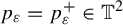














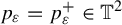






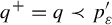





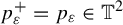






Claim 4.6. Let
$I\subset \mathcal {F}_1(p)$
 be given as above with length
$|I|=\delta _p$
 . Then, there exist constants
${\varepsilon }_0>0$
 and
$C>1$
 such that for every
${\varepsilon }\in (0,{\varepsilon }_0)$
 ,

where
$J_{\varepsilon }$
 is given as above.
Proof of Claim 4.6.
Let
$\bar {I}=h(I)$
 ,
$\bar {J}_{\varepsilon }=h(J_{\varepsilon })$
 ,
$\bar {p}=h(p)$
 ,
$\bar {w}=h(w)$
 ,
$\bar {p}_{\varepsilon }=h(p_{\varepsilon })$
 ,
$\bar {w}_{\varepsilon }=h(w_{\varepsilon })$
 , and
$\bar {q}=h(q)$
 . Denote the length of
$\bar {I}$
 by
$\bar {\delta }_p$
 . Note that

This implies that
$\bar {J}_{\varepsilon }$
 is a rigid translation of
$\bar {I}$
 , as A is linear. Hence, we have
${|\bar {J}_{\varepsilon }|=\bar {\delta }_p=|\bar {I}|}$
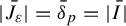 .
We will prove this claim in the
$cu$
 -DA case and
$sc$
 -DA case.
When f is
$cu$
 -DA, we assume that
$q=q^+$
 , as the case
$q=q^-$
 is similar. We consider three points
$q\prec q_1\prec q_2\prec q_3 \in \mathcal {F}^c_f(q)$
 such that:
-
• $h^{-1}\circ h(q_i)=\{q_i\}$
for
$i=1,2,3$
; -
• the point $\bar {q}_i=h(q_i)$
satisfies $$ \begin{align*}\frac{\bar{\delta}_p}{4} \leqslant d(\bar{q},\bar{q}_1) <\frac{\bar{\delta}_p}{3},\quad \frac{\bar{\delta}_p}{2} \leqslant d(\bar{q},\bar{q}_2) <\bar{\delta}_p,\quad 2\bar{\delta}_p\leqslant d(\bar{q},\bar{q}_3) <3\bar{\delta}_p. \end{align*} $$


This can be done by Lemma 2.12. Without loss of generality, we assume that

Denote by
$\bar {p}_{\varepsilon }'$
 and
$\bar {w}_{\varepsilon }'$
 the unique intersection points of local leaf
$\mathcal {L}^s(\bar {q})$
 with local leaves
$\mathcal {L}^u(\bar {p}_{\varepsilon })$
 and
$\mathcal {L}^u(\bar {w}_{\varepsilon })$
 , respectively. When
${\varepsilon }_0$
 is small enough, one has that for
${\varepsilon }<{\varepsilon }_0$
 ,

See Figure 6. It follows that

where
$p^{\prime }_{\varepsilon }$
 and
$w_{\varepsilon }'$
 are the unique intersection points of local leaf
$\mathcal {F}^c_f(q)$
 with local leaves
$\mathcal {F}_f^u(p_{\varepsilon })$
 and
$\mathcal {F}_f^u(w_{\varepsilon })$
 , respectively.
The choice of points
$q_1,q_2,q_3$
 . (Color online.)

Figure 6 Long description
The diagram consists of two panels connected by a horizontal arrow pointing right, labeled h.
Left Panel:
- A horizontal solid curve at the bottom is labeled F super u (q). A black dot on this curve is labeled q = q super plus.
- A vertical solid curve labeled F sub f super c (q) intersects the bottom curve at q.
- Two dashed horizontal curves cross the vertical curve. The lower dashed curve is labeled p sub epsilon = p sub epsilon super plus. The upper dashed curve is labeled w sub epsilon = w sub epsilon super minus.
- On the vertical curve, from bottom to top, are: a red cross p prime sub epsilon, a blue dot q sub 1, a blue dot q sub 2, a red cross w prime sub epsilon, and a blue dot q sub 3.
- A vertical line segment J sub epsilon connects the two dashed curves to the left of the vertical curve.
Right Panel:
- The structures are straightened into a Cartesian-like grid.
- The bottom horizontal line is L super u (q bar). The origin point is q bar.
- The vertical line is L super s (q bar).
- Two horizontal dashed lines represent the transformed curves. The lower one is p bar sub epsilon and the upper one is w bar sub epsilon.
- A vertical segment J bar sub epsilon connects these dashed lines.
- On the vertical axis, the points are mapped as: red cross p bar prime sub epsilon, blue dot q bar sub 1, blue dot q bar sub 2, red cross w bar prime sub epsilon, and blue dot q bar sub 3.
- Vertical dimensions are indicated on the right: the distance from q bar to q bar sub 1 is delta bar sub p all over 4, to q bar sub 2 is delta bar sub p all over 2, and to q bar sub 3 is 2 delta bar sub p. A bracket on the left indicates the total height delta bar sub p.
Let
$q',q_i'\ (i=1,2,3)$
 be the intersections of local leaf
$\mathcal {F}^c_f(p_{\varepsilon })$
 with local leaves
$\mathcal {F}_f^u(q), \mathcal {F}_f^u(q_i)$
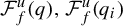 , respectively. Then, by the continuity of holonomy map along the unstable leaf
$\mathcal {F}^u_f(x)$
 for
$x\in \Lambda $
 , given a size
$\eta>0$
 of the local unstable foliation, one can get that
$d_{\mathcal {F}^u_f}(q',q_3')$
 has an upper bound
$C_2<+\infty $
 and
$d_{\mathcal {F}^u_f}(q_1',q_2')$
 has a lower bound
$C_1>0$
 , where
$C_1$
 and
$C_2$
 only depend on
$\eta $
 . This implies that the length
$|J_{\varepsilon }|$
 satisfies, for
${\varepsilon }<{\varepsilon }_0$
 ,

Now, let f be
$sc$
 -DA. Note that the semi-conjugacy h restricted to each stable leaf is in fact a homeomorphism. It is clear that there exists
$\delta>0$
 such that
$|J_{\varepsilon }|\geqslant \delta $
 for every
${\varepsilon }>0$
 . Otherwise, there exist
$w_{\varepsilon }$
 and
$q_{\varepsilon }$
 such that

It contradicts the continuity of h.
However, the length of
$J_{\varepsilon }$
 has an upper bound which is given by the lift on the universal cover. Indeed, let H be the lift of h. Then, there exists
$C_0$
 such that
$\|H-\mathrm {Id}_{\mathbb {R}^2}\|_{C^0}<C_0$
 . This implies that the lifts
$\tilde {w}_{\varepsilon },\tilde {p}_{\varepsilon }\in \mathbb {R}^2$
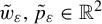 of
$w_{\varepsilon }, q_{\varepsilon }$
 satisfy
$d(\tilde {w}_{\varepsilon },\tilde {p}_{\varepsilon })<2C_0+\bar {\delta }_p$
 . Otherwise,

It contradicts the fact that
$|\bar {J}_{\varepsilon }|=\bar {\delta }_p$
 . Hence, the length
$|J_{\varepsilon }|$
 is uniformly bounded away from
$0$
 . This ends the proof of Claim 4.6.
Recall that for given
$\delta $
 , we fix
$\eta _0>0$
 such that for any
$x,y\in \mathbb {T}^2$
 with
$d(x,y)\leqslant \eta _0$
 , one has

Let
$B_{\eta _0}(p)$
 and
$B_{\eta _0}(q)$
 be the
$\eta _0$
 -balls of p and q, respectively. Here, we fix a
$\mathcal {F}_1$
 -foliation box
$D^+$
 of
$q=q^+$
 such that:
-
• $D^+\subset B_{\eta _0}(q) $
; -
• the boundaries of $D^+$
intersect with local leaf
$\mathcal {F}^c_f(q)$
at two points q and
$q_D\in \Lambda $
such that
$h^{-1}\circ h(q_D)=\{q_D\}$
and
${q\prec q_D}$
; -
• the boundaries of $D^+$
are leaves of foliation
$\mathcal {F}_1$
or
$\mathcal {F}_2$
.
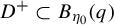


This can be done by Lemma 2.12. Similarly, when
$q=q^-$
 , we can define foliation box
$D^-$
 as the same above three items, but
$q_D\prec q$
 .
In the rest of the proof, we will consider the curves
$I\subset B_{\eta _0}(p)$
 and
$J_{\varepsilon } \in D^{\pm }$
 . Indeed, we have the following claim.
Claim 4.7. Let
$q=q^\sigma \ (\sigma =+ \ \mathrm {or}\ -)$
 . There exist
$\delta _p>0$
 and
${\varepsilon }_1>0$
 such that for I with
$|I|=\delta _p$
 and any
${\varepsilon }\in (0,{\varepsilon }_1)$
 , one has
$f^k(I)\subset B_{\eta _0}(p)$
 for every
$k\geqslant 0$
 , and
$J_{\varepsilon } \subset D^{\sigma }$
 .
Proof of Claim 4.7.
It is clear that when
$\delta _p$
 is small, we have
$I\subset B_{\eta _0}(p)$
 . For
$J_{\varepsilon }$
 , we just prove the claim for
$\sigma =+$
 and the proof of the other case is similar.
Let
$\bar {D}^+=h(D^+)$
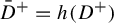 . Note that
$\bar {D}^+$
 has non-empty interior on
$\mathbb {T}^2$
 . Hence, when
$\delta _p$
 and
${\varepsilon }_1$
 are small enough, one has
$\bar {J}_{\varepsilon }\subset \mathrm {Int}\bar {D}^+$
 for
${\varepsilon }<{\varepsilon }_1$
 . By the construction of
$J_{\varepsilon }$
 and
$D^+$
 , we obtain
$J_{\varepsilon }\subset D^+$
 .
Note that we can also take an
$\mathcal {F}_1$
 -foliation box
$D^+_p$
 of
$p=p^+$
 , which satisfies three conditions of
$D^+$
 , but using p to replace q. Let
$\delta _p$
 be small such that
$I\subset D^+_p$
 . It follows from
$\bar {I}\subset \mathcal {L}^s(\bar {p})\cap h(D^+_p) $
 that
$A^k(\bar {I})\subset \mathcal {L}^s(\bar {p})\cap h(D^+_p)$
 for every
$k\geqslant 0$
 . Since the endpoints of
$f^k(I)$
 are
$f^k(p^+)$
 and
$f^k(w^-)$
 , one has
$f^k(I)\subset D^+_p\subset B_{\eta _0}(p)$
 . This ends the proof of Claim 4.7.
Now, we take
$\delta _p, I$
 and
${\varepsilon }_1$
 satisfying Claim 4.7. For
$q=q^\sigma \ (\sigma =+ \ \mathrm {or}\ -)$
 and
${\varepsilon }<{\varepsilon }_1$
 , we can define an
$\mathcal {F}_1$
 -foliation box
$D_{\varepsilon }^\sigma $
 just like the construction of
$D^\sigma $
 as follows:
-
• $D_{\varepsilon }^\sigma \subset B_{{\varepsilon }}(q) $
; -
• the boundaries of $D_{\varepsilon }^\sigma $
intersect with local leaf
$\mathcal {F}^c_f(q)$
at two points q and
$q_{\varepsilon }\in \Lambda $
such that
$h^{-1}\circ h(q_{\varepsilon })=\{q_{\varepsilon }\}$
; moreover, if
$q=q^+$
, then
$q\prec q_{\varepsilon }$
and if
$q=q^-$
, then
${q_{\varepsilon }\prec q}$
; -
• the boundaries of $D_{\varepsilon }^\sigma $
are leaves of foliation
$\mathcal {F}_1$
or
$\mathcal {F}_2$
.





Denote by

Then, for
$K_{\varepsilon }$
 (the specific replacement of
$k_{\varepsilon }$
 ), we choose a corresponding curve that is still denoted by
$J_{\varepsilon }$
 satisfying
$f^{K_{\varepsilon }}(I)=f^{K_{\varepsilon }}(J_{\varepsilon })$
 . Denote by
$N_{\varepsilon }\in \mathbb {N}$
 the first time such that
$f^{N_{\varepsilon }}(J_{\varepsilon })$
 is not contained in
$D^\sigma $
 , namely,

Claim 4.8. There exist constants
${\varepsilon }_2>0$
 and
$\alpha \in (0,1)$
 such that for every
${\varepsilon }\in (0,{\varepsilon }_2)$
 , one has

Proof of Claim 4.8.
We just prove this claim for
$q=q^+$
 and the proof of the other case is similar. By Lemma 2.12, when
${\varepsilon }_2<{\varepsilon }_1$
 is small enough, we have
$D_{\varepsilon }^+\subset D^+$
 for every
$0<{\varepsilon }<{\varepsilon }_2$
 .
Let
$\bar {D}^+_{\varepsilon }=h(D_{\varepsilon }^+)$
 . Note that
$\bar {D}^+_{\varepsilon }$
 and
$\bar {D}^+$
 are both
$\mathcal {L}^{s/u}$
 -foliation boxes of
$\bar {q}$
 with non-empty interior on
$\mathbb {T}^2$
 , since h preserves the leaves. For convenience, we can assume that
$\bar {D}^+_{\varepsilon }$
 and
$\bar {D}^+$
 are both squares with side lengths
$\bar {{\varepsilon }}$
 and
$\bar {\eta }_0$
 , respectively.
Denote by

It is clear that

where
$\gamma \in (0,1)$
 and
$C_A$
 are constants given in Lemma 2.3.
Denote by
$\bar {p}_{\varepsilon }'$
 the unique intersection point of local leaves
$\mathcal {L}^s(\bar {p}_{\varepsilon })$
 and
$\mathcal {L}^u(\bar {q})$
 . Denote by
$\bar {N}_{\varepsilon }$
 the first time such that
$A^{\bar {N}_{\varepsilon }}(\bar {p}_{\varepsilon }')$
 is not contained in
$\bar {D}^+_{\varepsilon }$
 , namely,

It follows from Claim 4.7 that
$\bar {J}_{\varepsilon }\subset \bar {D}^+$
 . Then, by the construction of the foliation box,
$\bar {D}^+_{\varepsilon }$
 and
$\bar {J}_{\varepsilon }$
 is a curve on a stable leaf, and one has

where
$\nu =\|A|_{L^u}\|>1$
 .
As a result, one has

Note that
$\bar {{\varepsilon }}$
 tends to
$0$
 as
${\varepsilon } \to 0$
 . Hence, when
${\varepsilon }_2$
 is small enough, one has

for every
${\varepsilon }\in (0,{\varepsilon }_2)$
 . By Lemma 2.3, one can take
$\gamma ={|}{\det} (A)|^{-\tfrac 12}$
 . Then, it follows that

since
$\nu>{|}{\det} (A)|>1$
 .
Let
$0<{\varepsilon }<\min \{{\varepsilon }_0,{\varepsilon }_1,{\varepsilon }_2\}$
 , where
${\varepsilon }_0, {\varepsilon }_1, {\varepsilon }_2$
 are given in Claims 4.6, 4.7, and 4.8, respectively. We are going to calculate the error between the lengths of
$f^{K_{\varepsilon }}(I)$
 and
$f^{K_{\varepsilon }}(J_{\varepsilon })$
 induced by the gap of Lyapunov exponents.
Note that

so by Claim 4.7, we have

However, by
$f^{i}(J_{\varepsilon })\subset B_{\eta _0}(q)$
 for
$0\leqslant i\leqslant N_{\varepsilon }-1$
 , we have

Although we have

and

we cannot calculate
$f^{K_{\varepsilon }}(J_{\varepsilon })$
 directly. Because
$J_{\varepsilon }$
 is not contained in
$\Lambda $
 for the
$cu$
 -DA case,
$f^k(J_{\varepsilon })$
 could not be in an
$\eta _0$
 -ball for some
$k>N_{\varepsilon }$
 .
This leads us to marking a specific iteration. We take
$K_0\in [N_{\varepsilon },K_{\varepsilon }]$
 such that
$K_0$
 is the last time k satisfying
$f^k(J_{\varepsilon })$
 is not in the
$\eta _0$
 -ball
$B_{\eta _0}(f^k(p_{\varepsilon }))$
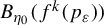 , namely,

Here, we claim that when
${\varepsilon }\to 0$
 (so
$K_{\varepsilon }\to +\infty $
 ), one has
$K_{\varepsilon }>N_{\varepsilon }$
 . Otherwise, if
${K_{\varepsilon }\leqslant N_{\varepsilon }}$
 , then

and

as
$ {\varepsilon }\to 0$
 . Here, recall that
$\delta <({\unicode{x3bb} _+-\unicode{x3bb} _-})/{4}$
 , and C is given in Claim 4.6. Therefore, we can assume
$K_{\varepsilon }>N_{\varepsilon }$
 when
${\varepsilon }$
 is small enough. Then, there are the following possibilities for
$K_0$
 .
(1) If
$K_0$
 does not exist (or
$K_0<N_{\varepsilon }$
 ), that is,
$f^{k}(J_{\varepsilon })\subset B_{\eta _0}(f^{k}(p_{\varepsilon }))$
 for every
${k\in [N_{\varepsilon },K_{\varepsilon }]}$
 , then one has

where
$\alpha $
 is given in Claim 4.8. Hence,

Since
$\delta < ({\alpha (\unicode{x3bb} _+-\unicode{x3bb} _-)})/{4}$
 and
$K_{\varepsilon }\to +\infty $
 as
${\varepsilon }\to 0$
 , one has

It contradicts the fact that
$f^{K_{\varepsilon }}(J_{\varepsilon })=f^{K_{\varepsilon }}(I)$
 .
(2) If
$K_0=K_{\varepsilon }$
 , then
$f^{K_{\varepsilon }}(J_{\varepsilon })\not \subset B_{\eta _0}(p)$
 since
$f^{K_{\varepsilon }}(p_{\varepsilon })=f^{K_{\varepsilon }}(p)=p$
 . It contradicts the fact that
$f^{K_{\varepsilon }}(J_{\varepsilon })=f^{K_{\varepsilon }}(I)\subset B_{\eta _0}(p)$
 , see Claim 4.7.
(3) If
$K_0\in [N_{\varepsilon },K_{\varepsilon })$
 , then
$f^k(J_{\varepsilon })\subset B_{\eta _0}(f^k(p_{\varepsilon }))$
 for
$k>K_0$
 . In addition,
$f^{K_0}(J_{\varepsilon })\not \subset B_{\eta _0}(f^{K_0}(p_{\varepsilon }))$
 implies
$f^{K_0+1}(J_{\varepsilon })>\eta _0$
 , so there exists a constant
$R_0>0$
 , which depends only on
$\eta _0$
 and
$\min _{x\in \mathbb {T}^2}\|Df|_{E_1(x)}\|$
 such that
$f^{K_0+1}(J_{\varepsilon })>R_0$
 . Thus, it follows that

Since
$\unicode{x3bb} _-<0$
 and
$1+K_0\geqslant N_{\varepsilon }\geqslant \alpha K_{\varepsilon }$
 , one has

Hence,

Since
$\unicode{x3bb} _-<0$
 and
$\delta < {-\alpha \unicode{x3bb} _-}/({4-2\alpha })$
 , one has

It contradicts the fact that
$f^{K_{\varepsilon }}(J_{\varepsilon })=f^{K_{\varepsilon }}(I)$
 .
All in all, we obtain the contradiction induced by the exponent gap. Hence,
$\unicode{x3bb} ^1(p)=\unicode{x3bb} ^1(q)$
 for any
$p,q\in \mathrm {Per}(f|_\Lambda )$
 . This ends the proof of Proposition 4.1.
Remark 4.9. We mention that through the whole proof of Proposition 4.1, the condition
$\unicode{x3bb} _-<0$
 is used only in calculating the error between
$|f^{K_{\varepsilon }}(I)|$
 and
$|f^{K_{\varepsilon }}(J_{\varepsilon })|$
 in the setting of
$cu$
 -DA endomorphisms with
$K_0\in [N_{\varepsilon },K_{\varepsilon })$
 . The existence of
$\unicode{x3bb} _-<0$
 will be shown later for the
$cu$
 -DA case in §6.
5 DA endomorphisms with stable bundles
In this section, we prove Theorem C, which focuses on the rigidity of stable Lyapunov exponents of
$sc$
 -DA endomorphisms on
$\mathbb {T}^2$
 . Moreover, by following Proposition 5.1, we give an example of the
$sc$
 -DA endomorphism on
$\mathbb {T}^2$
 , which is strictly semi-conjugate to its linearization. Further, even some rigidity assumption on a large invariant set cannot guarantee the existence of semi-conjugacy. Notice that this phenomenon is different from the
$cu$
 -DA case, where the semi-conjugacy must be injective; hence, the semi-conjugacy is a topological conjugacy (see Theorem B).
First, we prove Theorem C. Recall that
$f:\mathbb {T}^2\to \mathbb {T}^2$
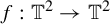 is a
$C^{1}$
 -smooth
$sc$
 -DA endomorphism and
$A:\mathbb {T}^2\to \mathbb {T}^2$
 is its hyperbolic linearization. When f is semi-conjugate to A via h, we denote by
$\Lambda :=\overline {\{x\in \mathbb {T}^2\mid h^{-1}\circ h(x)=\{x\}\}}$
 the closure of the h-injective points set.
Proof of Theorem C.
By Corollary 2.10 and Theorem A, the existence of semi-conjugacy and f being special are equivalent in the
$sc$
 -DA case. Moreover, by Proposition 2.11, we have
$\overline {\mathrm {Per}(f|_{\Lambda })}=\Lambda $
 . Hence, it suffices to prove the rigidity of stable Lyapunov exponents. By Proposition 4.1, we already have
$\unicode{x3bb} ^s(p,f)=\unicode{x3bb} ^s(q,f)\equiv \unicode{x3bb} $
 for any
$p,q\in \mathrm {Per}(f|_{\Lambda })$
 , so we prove
$\unicode{x3bb} =\unicode{x3bb} ^s(A)$
 .
Let
$\Gamma $
 be the lifting of
$\Lambda $
 on
$\mathbb {R}^2$
 . By Proposition 4.2, for any
${\varepsilon }>0$
 , one can find an adapted metric
$\|\cdot \|$
 such that

If
$|\unicode{x3bb} -\unicode{x3bb} ^s(A)|\neq 0$
 , one can pick
$\varepsilon \in (0,|\unicode{x3bb} -\unicode{x3bb} ^s(A)|)$
 . Then, on the one hand, for any
$y\in \mathcal {F}_F^s(x)\subset \Gamma $
 ,

On the other hand,

Note that for any
$k\in \mathbb {N}$
 ,

where
$C_H$
 is given in Proposition 2.5. Thus, one can get a contradiction from the quasi-isometric property of
$\mathcal {F}_F^s$
 .
Proposition D follows from the following result. Furthermore, as mentioned in Remark 1.8 and in the beginning of this section, we also construct an
$sc$
 -DA endomorphism that has constant periodic stable Lyapunov exponent in a large invariant set, but it is not semi-conjugate to its linearization. Precisely, we give the following extended result of Proposition D.
Proposition 5.1. Let
$A:\mathbb {T}^2\to \mathbb {T}^2$
 be an Anosov endomorphism with a non-trivial stable bundle. Then, there exists a
$C^\infty $
 -smooth
$sc$
 -DA endomorphism
$g_0:\mathbb {T}^2\to \mathbb {T}^2$
 such that:
-
(1) $g_0$
is semi-conjugate to A and any semi-conjugacy h homotopic to
$\mathrm {Id}_{\mathbb {T}^2}$
is not injective; -
(2) the set
$$ \begin{align*}\Lambda_{g_0}:=\overline{ \{ x\in\mathbb{T}^2\mid h^{-1}\circ h(x)=x \}}\neq \mathbb{T}^2,\end{align*} $$is a uniformly hyperbolic repeller.


Moreover, there exists a
$C^\infty $
 -smooth
$sc$
 -DA endomorphism
$g_1:\mathbb {T}^2\to \mathbb {T}^2$
 homotopic to A such that:
-
(1) the semi-conjugacy H guaranteed by Proposition 2.5 does not commute with the deck transformations, and $g_1$
is not special; -
(2) the set
$$ \begin{align*}\Gamma_{g_1}:=\{x\in\mathbb{R}^2\mid H^{-1}\circ H(x)=\{x\} \}\end{align*} $$is invariant and satisfies $\bar {\Gamma }_{g_1}+\mathbb {Z}^2=\bar {\Gamma }_{g_1}$
and
$H(\Gamma _{g_1})=\mathbb {R}^2$
;
-
(3) the set $\Lambda _{g_1}:=\pi (\bar {\Gamma }_{g_1})\subset \mathbb {T}^2$
is compact,
$g_1^{\pm 1}$
-invariant, and
$\mathcal {F}^s_{g_1}$
-saturated; -
(4) $\overline {\mathrm {Per}(g_1|_{\Lambda _{g_1}})}=\Lambda _{g_1}$
and
$\unicode{x3bb} ^s(p,g_1)=\unicode{x3bb} ^s(A)$
for any
$p\in \mathrm {Per}(g_1|_{\Lambda _{g_1}})$
.










Proof. The construction of
$g_0$
 is a modification for the DA diffeomorphism in [Reference Katok and Hasselblatt35, §17.2], but for completeness and some difference between diffeomorphisms and endomorphisms, we give the proof as follows.
Let
$A:\mathbb {T}^2\to \mathbb {T}^2$
 be a hyperbolic endomorphism with a non-trivial stable bundle. Assume that
$A(0)=0$
 . Let U be a neighborhood of
$0$
 and we can give a coordinates
$(x,y)$
 on U diagonalizing A on U such that

where

In particular, we assume that U is a square with the edge length
$\tfrac 12$
 centering
$0$
 .
Let
$\phi (t):\mathbb {R}\to [0,1]$
 be
$C^\infty $
 a bump function such that:
-
• $\phi (t)=1$
if
$|t|\leqslant \tfrac 18$
and
$\phi (t)=0$
if
$|t|\geqslant \tfrac 14$
; -
• $\phi (-t)=\phi (t)$
; -
• $-9<\phi '(x)<0$
when
$\tfrac 18<t<\tfrac 14$
.




Let
$g_0:\mathbb {T}^2\to \mathbb {T}^2$
 be given as:
-
• $g_0|_{\mathbb {T}^2\setminus U}=A|_{\mathbb {T}^2\setminus U}$
; -
• $g_0(x,y)=A(x,y)+(0,\unicode{x3bb} \phi (x)\phi (ky)y)$
for every
$(x,y)\in U$
,


where
$\unicode{x3bb} <0$
 and
$k\geqslant 1$
 are constants and given later.
It is clear that
$g_0$
 is
$C^{\infty }$
 . Note that we just perturb A along its unstable manifold
$\mathcal {L}^u$
 ; hence, the foliation
$\mathcal {L}^u$
 is
$g_0$
 -invariant and gives a
$Dg_0$
 -invariant bundle
$L^u$
 (may not be expanding under
$Dg_0$
 ). To construct the desired
$g_0$
 , we choose
$\unicode{x3bb} $
 and k satisfying the following claims.
Claim 5.2. There exist
$\unicode{x3bb} $
 and k such that:
-
(1) there exists fixed point $p\in U\setminus \{0\}$
with
$g_0(p)=p$
and
$p\in \mathcal {L}^u(0)$
; -
(2) there exists a $Dg_0$
-contracting cone field $$ \begin{align*} \mathcal{C}_a (z):=\{(x,y) \in T_z\mathbb{T}^2 \mid |y|\geqslant a|x| \}, \end{align*} $$namely, $Dg_0( \overline {\mathcal {C}_a (z)} ) \subset \mathrm {int}( \mathcal {C}_a (g_0(z)))$
;
-
(3) for every point $z\in \mathbb {T}^2$
and every vector
$v\notin \mathcal {C}_a (z)$
, one has
$\|D_zg_0v\|<\|v\|$
.


Note that if
$g_0$
 satisfies the second item, then there exists a
$Dg_0$
 -invariant dominated splitting
$T\mathbb {T}^2=E_{g_0}^1\oplus _< E_{g_0}^2$
 (see [Reference Crovisier and Potrie12]), in particular,
$E_{g_0}^2=L^u$
 . In addition,
$Dg_0$
 contracts the bundle
$E_{g_0}^1$
 by the third item. Hence,
$g_0$
 is a special
$sc$
 -DA endomorphism and we rewrite its partially hyperbolic splitting as

According to Theorem A,
$g_0$
 is semi-conjugacy to A. Let surjection
$h:\mathbb {T}^2\to \mathbb {T}^2$
 be homotopic to Id
$_{\mathbb {T}^2}$
 such that
$h\circ f=A\circ h$
 . Note that h preserves the center foliation, namely,
$h(\mathcal {F}_{g_0}^c(0))=\mathcal {L}^u(0)$
 , where
$\mathcal {F}_{g_0}^c$
 is the integral foliation of bundle
$E_{g_0}^c$
 . By the first item and the semi-conjugacy, it follows that
$h(p)=0$
 ; hence, h is not injective. Now, we check that
$g_0$
 satisfies the last three properties.
Proof of Claim 5.2.
The second and third items automatically hold for
$z\in \mathbb {T}^2\setminus U$
 since
$g_0|_{\mathbb {T}^2\setminus U}=A|_{\mathbb {T}^2\setminus U}$
 . Hence, we just focus on the perturbed neighborhood
$ U$
 . Let
$z=(x,y)\in U$
 . Then,

To get another fixed point on
$\mathcal {L}^u(0)$
 , let
$g_0(x,y)=(x,y)$
 and
$x=0$
 . Then, we get
$\phi (ky)=({1-\mu _2})/{\unicode{x3bb} }$
 . Hence, when
$\unicode{x3bb} < 1-\mu _2<0$
 , the equation
$\phi (ky)=({1-\mu _2})/{\unicode{x3bb} }\in [0,1]$
 has a solution
$y_0\in (0,{1}/{4k}]$
 . Then,
$p=(0,y_0)\in U$
 is a fixed point satisfying the first item.
Let
$(1,\pm a) \in \mathcal {C}_a(z)$
 . To prove the second item, we will find
$a\in \mathbb {R}_{\geqslant 0}$
 such that

By symmetry, we need only find a when
$x\geqslant 0$
 and
$y\geqslant 0$
 . Let

where

It is easy to get that
$B(x,y)\in [0,-({9}/{4k})\unicode{x3bb} ]$
 and
$C(x,y)\in [\mu _2+\unicode{x3bb} ,\mu _2-\tfrac 94\unicode{x3bb} ]$
 , when
${x\geqslant 0}$
 and
$y\geqslant 0$
 . Then, (5.2) follows from the following inequalities:

and

Recall that
$0<\mu _1<1$
 and notice that
$\unicode{x3bb} $
 can be close to
$1-\mu _2$
 . Thus, we can choose
$\unicode{x3bb} $
 such that
$\mu _2+\unicode{x3bb} -\mu _1>0$
 ; hence,
$C(x,y)-\mu _1\geqslant \mu _2+\unicode{x3bb} -\mu _1>0$
 . Then, (5.3) always holds when
$a>0$
 . However, the function

has an upper bound
$0<C_0(k)<+\infty $
 and
$C_0(k)\to 0$
 as
$k\to +\infty $
 . Hence, (5.4) always holds when
$a>C_0(k)$
 . As a result, we take
$a=2C_0(k)$
 , then
$\mathcal {C}_a$
 is the cone-field satisfying the second item.
To get the third property of
$g_0$
 , for
$z=(x,y)\in U$
 (we still assume that
$x,y\geqslant 0$
 ), we just need to show that every
$v=(1,b)\in T_z\mathbb {T}^2$
 not in
$\mathcal {C}_a(z)$
 will always satisfy the following inequality:

where for short, we denote
$B(x,y),C(x,y)$
 by
$B,C$
 , respectively. Then,

holds for all
$-2C_0(k) \leqslant b\leqslant 2C_0(k)$
 . This can be done since
$\mu _1\in (0,1)$
 ,
$C\in [\mu _2+\unicode{x3bb} ,\mu _2-\tfrac 94 \unicode{x3bb} ]$
 ,
$0\leqslant B\leqslant -({9}/({4k}))\unicode{x3bb} \to 0$
 , and
$C_0(k)\to 0$
 as
$k\to +\infty $
 for given
$\unicode{x3bb} < 1-\mu _2$
 .
From the choices of
$\unicode{x3bb} $
 in k of Claim 5.2,
$g_0$
 is an
$sc$
 -DA endomorphism. In addition, we further choose
$\unicode{x3bb} $
 and k such that
$\Lambda _{g_0}$
 is a uniformly hyperbolic repeller.
Claim 5.3. There exist
$\unicode{x3bb} $
 and k such that the set
$\Lambda _{g_0}$
 is a uniformly hyperbolic repeller.
Proof of Claim 5.3.
It suffices to prove that
$Dg_0|_{E^c(\Lambda _{g_0})}$
 is uniformly expanding.
Recall that
$E^c_{g_0}=L^u$
 ; hence, the conclusion follows from that there exists
$C_1>1$
 such that

Note that (5.5) always holds when
$(x,y)\in \mathbb {T}^2\setminus U$
 ; hence, we focus on U. Let

where
$V_x:=\{ y\in [-{1}/{4},{1}/{4}]\mid C(x,y)\leqslant 1\}$
 . By the compactness of
$\Lambda _{g_0}$
 and V, if
$V\subset \mathbb {T}^2\setminus \Lambda _{g_0}$
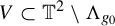 , then (5.5) holds.
Let
$\mu _1-\mu _2<\unicode{x3bb} <1-\mu _2$
 . Then,
$0$
 is a sink of
$g_0$
 . It is easy to find
$\unicode{x3bb} $
 and k such that
$(0,y_1)$
 and
$(0,y_2)$
 , with
$\phi (ky_i)=({1-\mu _2})/{\unicode{x3bb} }\ (i=1,2)$
 , are two saddle points on
$\mathcal {F}^c_{g_0}(0)$
 . Moreover, we can assume that
$(0,y_1), (0,y_2),(0,0)$
 are the only three fixed points on
$\mathcal {F}^c_{g_0}(0)\cap U$
 ; hence, the only three periodic points by monotonicity of
$g_0$
 along the center segment from
$(0,y_1)$
 to
$(0,y_2)$
 . Indeed, if
$(0,y)\in \mathcal {F}^c_{g_0}(0)\cap U$
 is a fixed point, then there exists
$n_0\in \mathbb {N}$
 such that

However, for given
$\mu _2, \unicode{x3bb} $
 , we can assume that U is small (let
$\phi $
 be suitable to U) and k is big enough such that
$|\mu _2y-y|$
 and
$|\unicode{x3bb} \phi (ky)y|$
 are small; hence,
$|\mu _2y+\unicode{x3bb} \phi (ky)y-y|<1$
 and
$n_0=0$
 .
Note that
$C(x,y)\leqslant 1$
 is equivalent to

when
$\phi (x)> 0$
 . In addition,
$(x,y)\notin V$
 when
$\phi (x)=0$
 . By (5.6), one can get that:
-
• if $|x_1|<|x_2|$
, then
$V_{x_2}\subset V_{x_1}$
; -
• if $g_0(x,y)=(x',y')$
and
$g_0(\{x\}\times V_x)=\{x'\}\times V_x'$
, then
$V_x' \subset V_{x'}$
by
$C(x,y)|_{V_x}\leqslant 1$
; -
• $\{0\}\times V_0\subset \mathbb {T}^2\setminus \Lambda _{g_0}$
. Indeed,
$V_0$
is a compact subset of the interval
$(y_1,y_2)$
on the center leaf
$\mathcal {F}^c_{g_0}(0)$
, so there is a neighborhood
$U_0$
of
$0$
on
$\mathcal {F}^s_{g_0}(0)$
such that
$\{x\}\times V_x\subset \mathbb {T}^2\setminus \Lambda _{g_0}$
for every
$x\in U_0$
.










There exists
$n\in \mathbb {N}$
 such that for every
$x\in \mathcal {F}^s_{g_0}(0)\cap U=\mathcal {L}^s(0)\cap U$
 , one has
$g_0^n(x)\in U_0$
 ; hence,

It follows that
$g_0^n(V)\subset \mathbb {T}^2\setminus \Lambda _{g_0}$
 and
$V\subset \mathbb {T}^2\setminus \Lambda _{g_0}$
 as
$\Lambda _{g_0}$
 is invariant.
Since we have proved that
$g_0$
 restricted on
$\Lambda _{g_0}$
 is uniformly hyperbolic, the stable set of a point
$z\in \Lambda _{g_0}$
 is the union of the stable manifold
$\mathcal {F}^s_{g_0}$
 of its generation set

that is,

Since
$\Lambda _{g_0}$
 is
$g_0^{\pm 1}$
 -invariant and
$\mathcal {F}^s_{g_0}$
 -saturated by Proposition 2.11, we have
$w\in P(z)\subset \Lambda _{g_0}$
 and
$\mathcal {F}^s_{g_0}(w)\subset \Lambda _{g_0}$
 . Then, we get that
$\Lambda _{g_0}$
 is a uniformly hyperbolic repeller.
Combining Claims 5.2 and 5.3, we obtain the existence of
$g_0$
 in Proposition 5.1.
Now, we are going to make another perturbation to obtain
$g_1:\mathbb {T}^2\to \mathbb {T}^2$
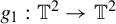 . Recall that

where h is a semi-conjugacy between
$g_0$
 and A. Note that
$\Lambda _{g_0}\neq \mathbb {T}^2$
 and
$\mathbb {T}^2\setminus \Lambda _{g_0}$
 has non-empty interior. By Theorem C and Proposition 2.11,

is a
$g_0^{\pm 1}$
 -invariant
$\mathcal {F}^s_{g_0}$
 -saturated set and
$\unicode{x3bb} ^s(p,g_0)=\unicode{x3bb} ^s(A)$
 for any
$p\in \mathrm {Per}(g|_{\Lambda _{g_0}})$
 . In fact, even for every
$p\in \mathrm {Per}(f)$
 , we can calculate directly that
$\unicode{x3bb} ^s(p,g_0)\equiv \log \mu _1$
 , since
$Dg_0$
 is of triangular form.
Let
$V\subset \mathbb {T}^2\setminus \Lambda _{g_0}$
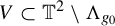 be an open set. Let
$g_1:\mathbb {T}^2\to \mathbb {T}^2$
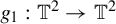 be a perturbation of
$g_0:\mathbb {T}^2\to \mathbb {T}^2$
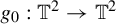 such that:
-
• $g_1|_{\mathbb {T}^2\setminus V}=g_0|_{\mathbb {T}^2\setminus V}$
; -
• $g_1$
is an
$sc$
-DA endomorphism; -
• $g_1$
is not special, namely, there is no
$Dg_1$
-invariant center bundle on
$T\mathbb {T}^2$
.


Note that
$g_0$
 is in fact a special Anosov endomorphism on
$\Lambda _{g_0}$
 , so the perturbation can be done by the same method of perturbing a special Anosov endomorphism to be non-special, see [Reference Przytycki49]. Then, there exists a semi-conjugacy
$H:\mathbb {R}^2\to \mathbb {R}^2$
 between
$G_1:\mathbb {R}^2\to \mathbb {R}^2$
 and
$A:\mathbb {R}^2\to \mathbb {R}^2$
 , the lifted maps of
$g_1$
 and A, respectively. Let
$H_0:\mathbb {R}^2\to \mathbb {R}^2$
 be a lifted map of h such that
$H_0\circ G_0=A\circ H_0$
 , where
$G_0:\mathbb {R}^2\to \mathbb {R}^2$
 is a lifted map of
$g_0$
 .
By Corollary F, H does not commute with the deck transformations. Let

Since
$\Lambda _{g_0}$
 is
$g_0^{\pm 1}$
 -invariant, we have
$\Lambda _{g_0}$
 is
$g_1^{\pm 1}$
 -invariant. Moreover,

where
$\widetilde {\Lambda }_{g_0}$
 is the lift of
$\Lambda _{g_0}$
 . Let
$\Lambda _{g_1}:=\pi (\overline {\Gamma }_{g_1})=\Lambda _{g_0}$
 . Then,
$g_1$
 restricted on
$\Lambda _{g_1}$
 and H restricted on
$\overline {\Gamma }_{g_1}$
 have the same properties as
$g_0|_{\Lambda _{g_0}}$
 and
$H_0|_{\widetilde {\Lambda }_{g_0}}$
 . This ends the proof of Proposition 5.1.
6 DA endomorphisms with unstable cone-fields
In this section, we will prove Theorem B and Corollary E, which focus on the rigidity of center Lyapunov exponents of
$cu$
 -DA endomorphisms on
$\mathbb {T}^2$
 .
Let f be a
$C^1$
 -smooth
$cu$
 -DA endomorphism on
$\mathbb {T}^2$
 and A be its hyperbolic linearization. Comparing with the
$sc$
 -DA case, there are more rigidity properties in the
$cu$
 -DA case; especially, the existence of semi-conjugacy h between f and A leads to h being a topological conjugacy and f being a special Anosov endomorphism. This rigidity result mainly follows from the next two lemmas. When f is semi-conjugate to A, let
$\Lambda \subset \mathbb {T}^2$
 be given in Proposition 2.11. The first one claims that the infimum of center Lyapunov exponents of periodic points on
$\Lambda $
 is negative so that we can apply Proposition 4.1.
Lemma 6.1. Assume that f is semi-conjugate to A. Then, there exists
$p\in \mathrm {Per}(f|_{\Lambda })$
 such that
$\unicode{x3bb} ^c(p,f)<0$
 . Moreover,
$\unicode{x3bb} ^c(q,f)=\unicode{x3bb} ^c(p,f)$
 for any
$p,q\in \mathrm {Per}(f|_{\Lambda })$
 . In particular, the set
$\Lambda $
 is a uniformly hyperbolic attractor.
In fact, the hyperbolic attractor
$\Lambda $
 is the whole torus.
Lemma 6.2. Assume that f is semi-conjugate to A. The hyperbolic attractor
$\Lambda $
 guaranteed by Lemma 6.1 is the whole
$\mathbb {T}^2$
 ; hence, f is a special Anosov endomorphism.
Combining Lemmas 6.1 and 6.2, we can get Theorem B immediately.
Proof of Theorem B.
By Lemmas 6.1 and 6.2, the
$C^{1}$
 -smooth
$cu$
 -DA f is indeed a special Anosov endomorphism. Then, by the result of [Reference An, Gan, Gu and Shi1, §3], one has that f is conjugate to A and

Note that we can also prove (6.1) directly. Since we already have
$\Lambda =\mathbb {T}^2$
 , we can apply Lemma 6.1 again to get that
$\unicode{x3bb} ^s(p,f)=\unicode{x3bb} ^s(q,f)$
 for any
$p,q\in \mathrm {Per}(f)$
 . Thus, by the same argument of the proof of Theorem C, we have
$\unicode{x3bb} ^s(p,f)\equiv \unicode{x3bb} ^s(A)$
 for any
$p\in \mathrm {Per}(f)$
 .
In [Reference An, Gan, Gu and Shi1], it is further proved that if f is a
$C^{1+}$
 -smooth Anosov endomorphism on
$\mathbb {T}^2$
 , then f is conjugate to its linearization if and only if f has the same periodic Lyapunov exponents on the stable bundle as those of its linearization. Combining this result and Theorem B, we can complete the proof of Corollary E. For convenience, we recall the four items in Corollary E as follows:
-
(1) f is semi-conjugate to A via $h:\mathbb {T}^2\to \mathbb {T}^2$
; -
(2) f is conjugate to A via $h:\mathbb {T}^2\to \mathbb {T}^2$
; -
(3) f is special;
-
(4) f is Anosov and $\unicode{x3bb} ^s(p,f)=\unicode{x3bb} ^s(A)$
for any
$p\in \mathrm {Per}(f)$
.




Proof of Corollary E.
By Theorems A and B, we have
$(3)\Longrightarrow (1)$
 and
$(1)\Longrightarrow (4)$
 . It follows from [Reference An, Gan, Gu and Shi1] that
$(4)\Longrightarrow (2)$
 , which requires that f is
$C^{1+}$
 -smooth. Finally, since
$(2)\Longrightarrow (1)$
 is trivial,
$(2)\Longrightarrow (1)\Longrightarrow (3)$
 can be done by Theorem B. Finally, by the result of [Reference An, Gan, Gu and Shi1, §§4 and 5], h is smooth along each leaf of the stable foliation.
Now, we prove Lemmas 6.1 and 6.2. For proving Lemma 6.1, we need to use the following Ruelle inequality for endomorphisms, which is given in [Reference Liu36], and here, we give an adaptation under the setting of this paper. Let f be a
$C^{1}$
 -smooth
$cu$
 -DA endomorphism and
$\mu $
 be an ergodic measure of f. Then, by [Reference Liu36, Remark 1.4],

where
$F_\mu (f)$
 is the folding entropy of
$(f,\mu )$
 whose definition and more properties can be found in [Reference Liu36, Reference Wu and Zhu62]. We note that the folding entropy is invariant under an isomorphism, namely, if
$(f_1,\mu _1)$
 is isomorphic to
$(f_2,\mu _2)$
 , then
$F_{\mu _1}(f_1)=F_{\mu _2}(f_2)$
 .
Proof of Lemma 6.1.
First, we prove the existence of periodic points in
$\Lambda $
 with negative center Lyapunov exponents. Let
$h:\mathbb {T}^2\to \mathbb {T}^2$
 be a semi-conjugacy between f and A. Let
$\mu =h^*(\mathrm {Leb})$
 , where Leb is the Lebesgue measure. Note that
$(f,\mu )$
 is isomorphic to
$(A,\mathrm {Leb})$
 . Indeed, the set

has
$\mu (\Lambda ')=\mathrm {Leb}(h(\Lambda '))=0$
 , since the intersection of
$\Lambda '$
 and every center leaf
$\mathcal {F}^c_f(x)$
 is the union of countable close intervals whose image under h is the set of countable points in
$\mathcal {L}^s(h(x))$
 . We also mention that the support of
$\mu $
 has supp
$(\mu )=\Lambda $
 by the same method in [Reference Ures61, §6].
Note that
$(A,\mathrm {Leb})$
 is ergodic and so is
$(f,\mu )$
 since
$(f,\mu )$
 is isomorphic to
$(A,\mathrm {Leb})$
 . Moreover,

Then, by (6.2), we can obtain
$\unicode{x3bb} ^c(\mu ,f)<0$
 . Indeed, if it is false, that is,
$\unicode{x3bb} ^c(\mu ,f)\geqslant 0$
 , then

This contradicts the fact that
$\unicode{x3bb} ^u(A)>\log (|\!\det (A)|)$
 . Now, by Lemma 4.3, there exists a sequence of periodic points
$p_n\in \Lambda $
 such that

Hence, there exists
$p\in \mathrm {Per}(f|_{\Lambda })$
 such that
$\unicode{x3bb} ^c(p,f)<0$
 . It follows from Proposition 4.1 that
$\unicode{x3bb} ^c(p,f)$
 is constant with respect to
$p\in \mathrm {Per}(f|_{\Lambda })$
 and we denote this constant by
$\unicode{x3bb} <0$
 .
Now, we are going to prove that
$\Lambda $
 is a uniformly hyperbolic attractor. In fact, by Proposition 4.2, there exists a Riemannian metric such that

This implies that
$f|_{\Lambda }$
 is uniformly hyperbolic. Moreover,
$\Lambda $
 is an attractor, since the unstable set of a point
$x\in \Lambda $
 is exactly the unstable manifold
$\mathcal {F}^u_f(x)$
 and
$\Lambda $
 is
$\mathcal {F}^u_f$
 -saturated by Proposition 2.11. This ends the proof of Lemma 6.1.
Finally, we prove
$\Lambda =\mathbb {T}^2$
 , which implies that f is a special Anosov endomorphism. Recall that this phenomenon does not happen in the
$sc$
 -DA case, see the counterexamples given in Proposition 5.1, where
$\Lambda $
 is a hyperbolic repeller but a proper subset of
$\mathbb {T}^2$
 . The following proof is inspired by [Reference Hammerlindl and Shi31, Proposition 4.10]. One can see the generation set

as the strong stable ‘leaf’ of
$x\in \Lambda $
 .
Proof of Lemma 6.2.
Note that we just need to prove
$\Lambda =\mathbb {T}^2$
 , then by Lemma 6.1, f is Anosov and f is special since
$f|_{\Lambda }$
 is special (Proposition 2.11) and
$\Lambda =\mathbb {T}^2$
 .
By contradiction, we assume that
$\Lambda \neq \mathbb {T}^2$
 , that is, there is a point
$x\in \mathbb {T}^2$
 with
${h^{-1}\circ h(x)\neq \{x\}}$
 . It is convenient to assume that x is the center point of the segment
$h^{-1}\circ h(x)\subset \mathcal {F}^c_f(x)$
 . Let
$\delta>0$
 such that the ball of x, with radius
$3\delta $
 in
$\mathbb {T}^2$
 , has

By the uniform continuity of h, there exists
${\varepsilon }_0>0$
 such that for any
$y,z\in \mathbb {T}^2$
 , if
$d(y,z)<{\varepsilon }_0$
 , then
$d(h(y),h(z))<\tfrac {1}{2}$
 . In addition, there exists
$0<{\varepsilon }<\min \{\delta ,{\varepsilon }_0\}$
 such that the
${\varepsilon }$
 -neighborhood of
$\Lambda $
 has

since
$\Lambda $
 is a hyperbolic attractor. It follows that

Indeed, if there exist
$k_0 \in \mathbb {N}$
 and
$y_0\in \mathbb {T}^2$
 such that
$y_0\in f^{-k_0}(B_\delta (z))\cap (B_{\varepsilon }(\Lambda ))$
 , then

This contradicts (6.3). Hence, for every
$k\in \mathbb {N}$
 ,
$x_{-k}\in f^{-k}(x)$
 , and
$x_{-k}'=h(x_{-k})$
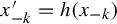 , we have

where
$\mathcal {L}^u(x_{-k}',1)$
 is the local leaf of
$\mathcal {L}^u(x_{-k}')$
 centered at
$x_{-k}'$
 with length smaller than
$1$
 .
Note that we can choose infinitely many distinct preimages
$x^{\prime }_{-k_i}\ (i\in \mathbb {N})$
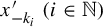 of
$x'$
 under A satisfying

Indeed, we can get these points
$x_{-k_i}'$
 as follows. Let
$x^{\prime }_{-k_1}=x^{\prime }_{-1}\in A^{-1}(x')$
 . There is a small size
$0<\eta \ll 1$
 such that

By the denseness of preimage sets (Lemma 2.3), we can take

for some
$k_2\in \mathbb {N}$
 . By induction, we can take

for each
$i\geqslant 2$
 and some
$k_i>k_{i-1}$
 . By (6.8), these points
$x_{-k_i}\ (i\in \mathbb {N})$
 satisfy (6.7).
Combining (6.6) and (6.7), we obtain that

This is impossible, since the volume of a ball
$ B_{\varepsilon }(x_{-k_i})\ (i\in \mathbb {N})$
 with radius
${\varepsilon }$
 has a lower bound.
Thus, h is injective and
$\Lambda =\mathbb {T}^2$
 . This ends the proof of Lemma 6.2.
Remark 6.3. We mention that the method in the proof of Lemma 6.2 is invalid in the
$sc$
 -DA case. In this case, the set
$\Lambda $
 may not be a repeller, since one can get the information of
$Df|_{E_f^s(\Lambda )}$
 (see Theorem C), but has no idea about
$Df|_{E_f^c(\Lambda )}$
 . Hence, one cannot get a similar property as (6.4). Furthermore, even if
$\Lambda $
 is a hyperbolic repeller (e.g., the
$\Lambda _{g_0}$
 constructed in Proposition 5.1), one can have
$B_{\varepsilon }(\Lambda )\subset f^k( B_\delta (\Lambda ) )$
 for all
$k\in \mathbb {N}$
 instead of (6.4), but this still does not imply that
$f^{-k}(B_{\varepsilon }(\Lambda ))\subset B_\delta (\Lambda ) $
 for all
$k\in \mathbb {N}$
 . Thus, one cannot get
$f^k(B_\delta (x))\cap B_{\varepsilon }(\Lambda )=\emptyset $
 for all
$k\in \mathbb {N}$
 as a replacement of (6.5) to show that
$\Lambda $
 is the whole torus.
7 Applications for the volume-preserving case
In this section, we prove Corollaries G and I, and we also give an example of a volume-preserving Anosov endomorphism on the torus whose Jacobian is not constant on periodic points.
First, we give the following property on the periodic boundaries. A point p is called a pre-periodic point of f if there is
$n\in \mathbb {N}$
 such that
$f^n(p)\in \mathrm {Per}(f)$
 . Let
$\Lambda \subset \mathbb {T}^2$
 be given in Proposition 2.11. Recall that the boundaries of sets
$\Lambda $
 and
$\mathbb {T}^2\setminus \Lambda $
 are hyperbolic leaves. Note that
$x\in \partial (\mathbb {T}^2\setminus \Lambda )$
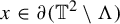 if and only if
$h^{-1}\circ h(x)\neq \{x\}$
 and
$x\in \Lambda $
 .
Lemma 7.1. Let
$f:\mathbb {T}^2\to \mathbb {T}^2$
 be a
$C^{1}$
 -smooth
$sc$
 -DA endomorphism semi-conjugate to its linearization
$A:\mathbb {T}^2\to \mathbb {T}^2$
 via
$h:\mathbb {T}^2\to \mathbb {T}^2$
 . Let
$\Lambda \subset \mathbb {T}^2$
 be given in Proposition 2.11 and
$\Lambda \neq \mathbb {T}^2$
 . If one of the following conditions holds:
-
(1) there exists $\unicode{x3bb}>0$
such that
$\unicode{x3bb} ^c(p,f)>\unicode{x3bb} $
for any
$p\in \mathrm {Per}(f|_{\Lambda })$
; -
(2) the non-wandering set $\Omega (f)=\mathbb {T}^2$
,




then, each stable leaf of the boundary
$\partial (\mathbb {T}^2\setminus \Lambda )$
 admits a unique pre-periodic or periodic point.
Proof. By Theorem C, f is special and admits an invariant center bundle
$E^c_f$
 that is integrable to foliation
$\mathcal {F}^c_F$
 . Without loss of generality, let f be orientation-preserving when restricted on
$\mathcal {F}^c_F$
 .
We consider the first condition. Let
$\unicode{x3bb}>0$
 such that
$\unicode{x3bb} ^c(p,f)>\unicode{x3bb} $
 for all
$p\in \mathrm {Per}(f|_{\Lambda })$
 .
Claim 7.2. There exists
$\eta>0$
 such that for any
$x\in \Lambda $
 , the length of any component
$I_{k}$
 of
$f^{-k}(\mathcal {F}^c_f(x,\eta ))$
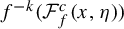 goes to
$0$
 , that is,

In particular, the center leaf of a point in
$\Lambda $
 with size
$\eta $
 is in fact an unstable manifold.
Proof of Claim 7.2.
According to Lemma 4.3, for every ergodic measure
$\mu $
 supported on
$\Lambda $
 , one has
$\unicode{x3bb} ^c(\mu ,f)\geqslant \unicode{x3bb} $
 . By the same construction of the adapted metric in Proposition 4.2, there exists a Riemannian metric such that

Then, there exists
$\eta>0$
 such that for any
$x\in \Lambda $
 and any
$y\in \mathcal {F}^c_f(x,\eta )$
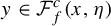 , one has

Recall that the set
$\Lambda $
 is
$f^{\pm }$
 -invariant. Hence, the constant
$\eta $
 is the size of unstable manifolds.
Let
$a=a^-\in \partial (\mathbb {T}^2\setminus \Lambda )$
 and
$\eta>0$
 be given in Claim 7.2. Let J be an open interval on
$\mathcal {F}^c_f(a,\eta )$
 such that it has an endpoint
$a^-$
 and
$J\subset \mathbb {T}^2\setminus \Lambda $
 . Considering the stable manifold of J,

there exists
$C_0>0$
 such that for every
$k\in \mathbb {N}$
 , the volume of the set
$f^k(\mathcal {F}^s_f(J))$
 is bigger than
$C_0$
 . Indeed, on the one hand, the length of curve
$f^k(J)$
 has a lower bound by Claim 7.2. On the other hand, the stable bundle
$E^s_f$
 is uniformly transverse to the center bundle
$E^c_f$
 . Thus, we can take a curve
$J_k\subset f^k(J)$
 with uniform length and a stable foliation box of
$J_k$
 with uniform size. Then, the volume of this foliation box gives the lower bound
$C_0$
 . If
$\mathcal {F}^s_f(a)$
 is neither a pre-periodic leaf nor a periodic leaf, then one has

Indeed, since f preserves the orientation of
$\mathcal {F}^c_f$
 , the point

is the negative endpoint of the curve
$h^{-1}\circ h (f^i(a))$
 for all
$i\in \mathbb {N}$
 . If (7.1) is not true, that is, there are
$i_0\neq j_0\in \mathbb {N}$
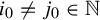 such that

then we have

This contradicts the fact that

since the sets
$\Lambda $
 (including
$\mathcal {F}^s_f(a)$
 ) and
$\mathbb {T}^2\setminus \Lambda $
 (including
$\mathcal {F}^s_f(J)$
 ) are
$f^{\pm }$
 -invariant.
Combining (7.1) and the fact that the volume of
$f^k(\mathcal {F}^s_f(J))$
 has lower bound
$C_0$
 , the volume of the union of sets
$f^k(\mathcal {F}^s_f(J))$
 is infinite. However, this is impossible. Thus,
$\mathcal {F}^s_f(a)$
 is a pre-periodic leaf or periodic leaf and admits a unique pre-periodic or periodic point.
Now, we consider the other case. Let
$\Omega (f)=\mathbb {T}^2$
 . In this case, the proof is inspired by [Reference Rodriguez Hertz, Rodriguez Hertz and Ures53, Proposition A.5]. Let
$a=a^-\in \partial (\mathbb {T}^2\setminus \Lambda )$
 . Then, there exists a close interval I on
$\mathcal {F}^c_f(a)$
 with
$I\setminus \{a\}\subset \mathbb {T}^2\setminus \Lambda $
 . Take a stable foliation box
$U_I$
 of I. Note that
$U_I\subset \mathbb {T}^2\setminus \Lambda $
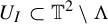 is an open set in
$\mathbb {T}^2$
 , and there are
$x\in U_I$
 and
$k\in \mathbb {N}$
 such that
$f^k(x)\in U_I$
 . Let y be the unique intersection point of local leaves
$\mathcal {F}^s_f(a)$
 and
$\mathcal {F}^c_f(x)$
 . Then, one has
$y\in \Lambda $
 , since
$\Lambda $
 is
$\mathcal {F}^s_f$
 -saturated.
We claim
$f^k(y)\in \mathcal {F}^s_f(a)$
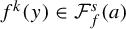 . Indeed, one has
$f^k(y) \notin U_I$
 as
$\Lambda $
 is invariant. If
${f^k(y)\notin \mathcal {F}^s_f(a)}$
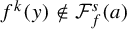 , then the interval
$ f^k(I\setminus \{a\})$
 on the leaf
$\mathcal {F}^c_f(f^k(x))$
 intersects with
$\mathcal {F}^s_f(a)$
 at at least one point
$z\in \Lambda $
 . However, this is impossible, since
$z\in f^k(I\setminus \{a\})$
 and
$f^k(I\setminus \{a\})\cap \Lambda =\emptyset $
 . So, one has
$y, f^k(y)\in \mathcal {F}^s_f(a)$
 . Finally, by the contraction of a stable leaf, there exists exactly one periodic point on
$\mathcal {F}^s_f(a)$
 .
Remark 7.3. Note that the center leaf in Claim 4.4 is just a half leaf of a boundary point, so we cannot apply it to the proof of Lemma 7.1 directly.
Proposition 7.4. Let
$f:\mathbb {T}^2\to \mathbb {T}^2$
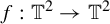 be a
$C^{1}$
 -smooth
$sc$
 -DA endomorphism semi-conjugate to its linearization
$A:\mathbb {T}^2\to \mathbb {T}^2$
 . If f satisfies one of the following conditions:
-
(1) there exists $\unicode{x3bb}>0$
such that
$\unicode{x3bb} ^c(p,f)>\unicode{x3bb} $
for any
$p\in \mathrm {Per}(f)$
; -
(2) f is volume-preserving,


then, f is a special Anosov endomorphism and
$\unicode{x3bb} ^s(p,f)=\unicode{x3bb} ^s(A)$
 for any
$p\in \mathrm {Per}(f)$
 .
Proof. First, we prove that the set
$\Lambda $
 given in Theorem C (see also Proposition 2.11) is in fact
$\mathbb {T}^2$
 .
Note that when f is volume-preserving, the non-wandering set of the
$sc$
 -DA will be
$\mathbb {T}^2$
 . So, by Lemma 7.1, both conditions imply that each stable leaf of the boundary
$\partial (\mathbb {T}^2\setminus \Lambda )$
 admits a unique pre-periodic or periodic point. For convenience, let
$p^+\in \partial (\mathbb {T}^2\setminus \Lambda )$
 be fixed. Then,
$p^-\neq p^+$
 is the other endpoint of
$h^{-1}\circ h(p^+)$
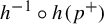 . Denote by
$I_p\subset \mathbb {T}^2\setminus \Lambda $
 the open interval on
$\mathcal {F}^c_f(p^+)$
 with endpoints
$p^\pm $
 , then we have
$f(\bar {I}_p)=\bar {I}_p$
 . Now, we deal with these two cases.
(1) Let f satisfy the first condition, namely, there exists
$\unicode{x3bb}>0$
 such that
$\unicode{x3bb} ^c(p,f)>\unicode{x3bb} $
 for any
$p\in \mathrm {Per}(f)$
 . Note that
$f:\bar {I}_p\to \bar {I}_p$
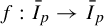 is a
$C^1$
 -smooth orientation-preserving map with

This implies that there exists a fixed point
$z_1\in I_p$
 . By
${\log \|Df|_{E^c_f(z_1)}\|> \unicode{x3bb} >0}$
 , there exists another fixed point
$z_2\in I_p$
 between
$p^-$
 and
$z_1$
 . Repeating this, we get infinitely many fixed points
$z_n$
 on
$I_p$
 with an accumulation point
$z\in \bar {I}_p$
 . Thus,
$\|Df|_{E^c_f(z)}\|=1$
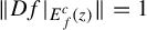 by the definition of derivative. It contradicts the assumption
$\log \|Df|_{E^c_f(z)}\|> \unicode{x3bb} >0$
 .
(2) Let f be volume-preserving. Consider the open interval
$I_p\subset \mathbb {T}^2\setminus \Lambda $
 and let

be a stable foliation box of
$\bar {I}_p$
 with the volume
$C_{\varepsilon }$
 . Then, by the contraction of stable leaves, the component of
$f^{-1}(U)$
 containing
$I_p$
 has a volume bigger than
$C_{\varepsilon }$
 . This contradicts the assumption of the volume-preserving property of f.
Hence, we get that
$\Lambda =\mathbb {T}^2$
 . In particular, f is indeed conjugate to A. By Theorem C, f is a special
$sc$
 -DA endomorphism and
$\unicode{x3bb} ^s(p,f)=\unicode{x3bb} ^s(A)$
 for any
$p\in \mathrm {Per}(f)$
 .
Next, we prove that f is Anosov.
Note that if f satisfies the first condition, namely, the infimum of the periodic center Lyapunov exponents is strictly bigger than
$0$
 , one can choose a Riemannian metric such that f is expanding on
$E^c_f$
 by a similar argument of Proposition 4.2. Notice that f has the shadowing property by inheriting from A via the conjugacy; this situation is actually easier than that of the non-uniformly shadowing property (Lemma 4.3), which we used in the proof of Proposition 4.2. Thus, the first condition further implies that f is Anosov.
The rest of the proof is to show that if f preserves a volume measure m, then f is also Anosov. Let
$\rho :\mathbb {T}^2\to \mathbb {R}_+$
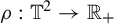 be the density of m, that is,
$dm(x)=\rho (x)d\mathrm {Leb}(x)$
 . Let
$\unicode{x3bb} ^s(A)=-\mu <0$
 . Recall that for any
$p\in \mathrm {Per}(f)$
 ,
$\unicode{x3bb} ^s(p,f)=\unicode{x3bb} ^s(A)=-\mu $
 . It suffices to prove

So, we will reduce the volume-preserving condition to the first case and conclude that f is Anosov.
For any point
$x\in \mathbb {T}^2$
 , let
$B_{\varepsilon }(p)$
 be the open ball centered at p with small radius
${\varepsilon }>0$
 . Then, for each periodic point
$p\in \mathrm {Per}(f)$
 of period k, one has

for some
$x_{\varepsilon }\in B_{\varepsilon }(p)$
 . Since f is volume-preserving,

Hence,
$\mathrm {Jac}(Df^k(x_{\varepsilon }))({\rho (f^k(x_{\varepsilon }))}/{\rho (x_{\varepsilon })})\geqslant 1$
 . Let
${\varepsilon }\to 0$
 . Then,
$x_{\varepsilon }\to p$
 and
$\mathrm {Jac}(Df^k(p)) \geqslant 1$
 . Namely,
$\unicode{x3bb} ^s(p,f)+\unicode{x3bb} ^c(p,f)\geqslant 0$
 . This gives us (7.2). Thus, f is Anosov when it is volume-preserving.
Now, we can obtain Corollary G from Proposition 7.4 immediately.
Proof of Corollary G.
The proof is similar to the proof of Corollary E. In fact, we just need to replace Theorem B by Proposition 7.4.
Now, we prove Corollary I. It should be mentioned here that though the constant periodic Jacobian data imply the existence of an invariant volume measure for toral Anosov endomorphisms, we cannot use this result under the assumption of Corollary I, where f is not a priori Anosov. This indicates the important role of Proposition 7.4 as well.
Proof of Corollary I.
Note that for any
$n\in \mathbb {N}$
 and
$p\in \mathrm {Fix}(f^n)$
 , one has

and
$Df|_{E^s_f}$
 is uniformly contracting, so there exists
$\unicode{x3bb}>0$
 with
$\unicode{x3bb} ^c(p,f)>\unicode{x3bb} $
 . Then, by Proposition 7.4, f is a special Anosov endomorphism. Thus, according to [Reference Gu and Shi26, Theorem 1.3], f is smoothly conjugate to A with the regularity we desired. It follows from the smooth conjugacy that f inherits the volume-preserving property from A.
Finally, we give a volume-preserving Anosov endomorphism that has no Jacobian rigidity.
Example 7.5. A volume-preserving Anosov endomorphism
$f:\mathbb {T}^2\to \mathbb {T}^2$
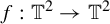 without Jacobian rigidity.
We start with a linear hyperbolic endomorphism. Let

It is clear that
$\deg (A) = \det (A) = 2$
 and A has a unique fixed point
$O_1 = (0,0)^T$
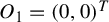 . Then,
$A^{-1}(O_1)$
 consists of two points
$O_1$
 and
$O_2 = (\tfrac 12, \tfrac 12)^T$
 . Let
$U_1$
 and
$U_2$
 be two neighborhoods of points
$O_1$
 and
$O_2$
 , respectively, such that

where
$U_0$
 is a small neighborhood of
$O_1$
 such that
$A|_{U_1}$
 and
$A|_{U_2}$
 are bijections onto
$U_0$
 , and there exists a periodic orbit of A, say
$\mathrm {Orb}_A(p)$
 , disjoint from
$U_i$
 , for all
$i = 0,1,2$
 .
Let
$v_u$
 be the unit eigenvector corresponding to the eigenvalue
$\unicode{x3bb} _u = 2 + \sqrt {2}$
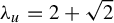 . Let
$\eta : U_0 \to \mathbb {R}$
 be a bump function on
$U_0$
 such that
$\eta (O_1) = 0$
 and
$\nabla \eta (O_1) = v_u \neq 0$
 . We define a vector field
$X: U_0 \to \mathbb {R}^2$
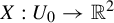 strictly aligned with the unstable manifold of A:

Note that
$O_1$
 is a singularity of X and its divergence is given by
$\mathrm {div}X(x) = \unicode{x3bb} _u (\nabla \eta (x))^T v_u$
 . Then, we perturb the linear inverse branches of A with
$B_i=(A|_{U_i})^{-1}:U_0\to U_i$
 for
$i=1,2$
 , using the induced maps of X. Specifically, we consider two maps

where
$\varepsilon> 0$
 is small and
$i = 1,2$
 . Let
$f: \mathbb {T}^2 \to \mathbb {T}^2$
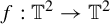 be such that

When
$\varepsilon> 0$
 is small enough, f is a smooth Anosov endomorphism with a
$Df$
 -invariant unstable bundle
$E_f^u = E_A^u$
 . Note that f is topologically conjugate to A, while there is no smooth conjugacy between f and A. To the end, we show that f is volume-preserving, but has no Jacobian rigidity.
By Sylvester’s determinant identity for rank-1 updates (that is,
$\det (I + uv^T) = 1 + v^T u$
 ), the Jacobian of
$g_i$
 can be explicitly computed. Using the chain rule on
$g_i(x)$
 , we have

where A is regarded as a matrix, then, taking the determinant of both sides, we can get

Note that the divergence of the vector field is exactly
$\mathrm {div}X(x) = \mathrm {Tr}(DX(x)) = \unicode{x3bb} _u (\nabla \eta (x))^T v_u$
 , so the expression simplifies to

Moreover, by
$\mathrm {div}X(O_1) = \unicode{x3bb} _u \neq 0$
 , we obtain

while we have
$g_1(O_1) = B_1(O_1) = O_1$
 and
$f(O_1) = O_1$
 by
$X(O_1) = 0$
 . However, since
$\mathrm {Orb}_A(p)$
 is disjoint from the perturbation regions, we have
$p \in \mathrm {Per}(f)$
 and
$\det (Df|_{\mathrm {Orb}_f(p)}) \equiv \det (A) = 2$
 . Thus, f has different period-averaged Jacobians at
$O_1, p$
 .
Furthermore, for any point
$x \in \mathbb {T}^2$
 , let
$f^{-1}(x) = \{x_1, x_2\}$
 . On the one hand, for
$x \notin U_0$
 ,

On the other hand, for
$x \in U_0$
 ,

Acknowledgements
The authors would like to thank Yi Shi for suggesting this rigidity problem, which is motivated by a question of Jérôme Buzzi at the conference of Beyond Uniform Hyperbolicity (2023). The authors would also like to thank Raúl Ures for comments and suggestions on the preliminary version of this paper, and anonymous referees for comments and suggestions that were helpful to improve this paper. This work was supported by National Key R&D Program of China (2021YFA1001900). R.G. was partially supported by NSFC (12571203) and the New Cornerstone Science Foundation through the New Cornerstone Investigator Program, and M.X. was partially supported by NSFC (Nos. 12161141002, 12501238) and the Fundamental Research Funds for the Central Universities (DUT24RC(3)112).