2. Scaling formulae and slice tilting

The inhomogeneous parameters associated with the electron beam transverse dimensions and divergences are specified by the identities

(2.1)\begin{equation} \left. \begin{gathered} \tilde{\mu}_{\eta'}=\frac{\varepsilon_{\eta}}{\beta_{\eta}}\frac{\gamma^{2}}{\rho}\frac{1}{\left(1+\dfrac{K^{2}}{2}\right)},\\ \tilde{\mu}_{\eta}=\varepsilon_{\eta}\frac{\gamma^{2}}{\rho}\frac{1}{\left(1+\dfrac{K^{2}}{2}\right)}\frac{\left(\gamma_{T}^{*}\right)^{2}}{\gamma_{\eta}}, \end{gathered} \right\} \end{equation}

where $\eta$ indicates the transverse dimensions $x,y$, $\gamma$ is the electron relativistic factor, $\lambda _{u}$ the undulator period and $B_{0}$ the peak of the on-axis magnetic field. Here $\beta _{\eta },\gamma _{\eta }$ are the matching Twiss parameters and $\beta _{\eta }^{*},\gamma _{\eta }^{*}$ denote the Twiss parameters for matching to the undulator natural focusing (NFTP). We use $a_{w}=K/\sqrt {2}$ for planar undulators and $a_{u}=K$ for helical undulators where $K={\lambda _{u}[\textrm {cm}]B_{0}[\textrm {KG}]}/{10.71}$ is the undulator strength parameter.

The Pierce parameter $\rho$, expressed in practical units, is

(2.2)\begin{equation} \left. \begin{gathered} \rho\simeq\frac{8.36\times10^{-3}}{\gamma}\left[J\left(\frac{A}{m^{2}}\right)\left(\lambda_{u}(\textrm{cm})\,Kf_{b}(K)\right)^{2}\right]^{{1}/{3}},\\ J=\frac{I}{2{\rm \pi}\sigma_{x}\sigma_{y}},\\ \sigma_{\eta}=\sqrt{\beta_{\eta}\varepsilon_{\eta}}, \end{gathered} \right\} \end{equation}

where $J$ is the current density, with $I$ the bunch current and $\sigma _{\eta }$ the bunch transverse root-mean-square (rms) size ($\eta =x,y$), and $f_{b}$ is the Bessel factor ($f_{b}=1$ for helical undulator, $f_{b}=J_{0}(\xi )-J_{1}(\xi )$ for linear undulator, with $J_{0}$ and $J_{1}$ the Bessel functions of order zero and one, and $\xi =({1}/{4})K^{2}{(1+{K^{2}}/{2})}^{-1}$). From here on, the case of a linear undulator (hence, $a_{w}=K/\sqrt {2}$) is considered, but the treatment remains valid also for a helical undulator.

We consider in the following that the average transverse sizes of the beam in the two radial and vertical directions are the same in the interaction region, ${\sigma }_{x}={\sigma }_{y}$. This condition is realistic in an undulator magnetic lattice by imposing, as a matching condition, that the difference between the $x$ and $y$ size of the beam has to be minimized (Quattromini et al. Reference Quattromini, Artioli, Di Palma, Petralia and Giannessi2012). In addition, we assume a beam with identical transverse emittances in both radial and vertical directions so that ${\varepsilon }_{x}={\varepsilon }_{y}$.

For this reason, from (2.2) we can define a value of emittance $\varepsilon$, beam size $\sigma$ and the Twiss parameter ${\beta }_{\eta },{\alpha }_{\eta },{\gamma }_{\eta }$ in such a way that

(2.3)\begin{equation} \left. \begin{gathered} {\varepsilon}_{x}={\varepsilon}_{y}=\varepsilon,\\ {\sigma}_{x}={\sigma}_{y}=\sigma,\\ {\beta}_{x}={\beta}_{y}={\beta}_{T},\\ {\gamma}_{x}={\gamma}_{y}={\gamma}_{T},\\ {\alpha}_{x}={\alpha}_{y}={\alpha}_{T}. \end{gathered} \right\} \end{equation}

As we show in the following, a crucial role is played by $\beta _{T},\gamma _{T}$ and by the NFTP linked to the undulator period and strength by the relations

(2.4a,b)\begin{equation} \gamma_{T}^{*}=\frac{1}{\beta_{T}^{*}},\quad \beta_{T}^{*}=\frac{\gamma\,\lambda_{u}}{{\rm \pi}\,K}. \end{equation}

Before proceeding further, let us note that, from (2.2) and with the assumption in (2.3), the Pierce parameter exhibits the following dependence on the beam current density

(2.5)\begin{equation} \rho\propto J^{{1}/{3}}=\left(\frac{I}{2{\rm \pi}\sigma^{2}}\right)^{{1}/{3}}. \end{equation}

Therefore, we define

(2.6)\begin{equation} \rho=\rho^{*}\left(\frac{\beta_{T}^{*}}{\beta_{T}}\right)^{{1}/{3}} \end{equation}

with $\rho ^{*}$ being the Pierce parameter calculated with a current density corresponding to the NFTP.

It is convenient to write (2.1) in the more useful form

(2.7)\begin{equation} \left. \begin{gathered} {\tilde{\mu}_{x'}=\tilde{\mu}_{x'}^{*}\left(\frac{\beta_{T}^{*}}{\beta_{T}}\right)^{{2}/{3}}},\\ {\tilde{\mu}_{x}=\tilde{\mu}_{x'}^{*}\left(\frac{\beta_{T}^{*}}{\beta_{T}}\right)^{-{2}/{3}}\frac{1}{\beta_{T}^{*}\gamma_{T}}=\frac{\tilde{\mu}_{x'}^{*}}{1+\alpha_{T}}\left(\frac{\beta_{T}^{*}}{\beta_{T}}\right)^{-{2}/{3}}},\\ {\tilde{\mu}_{x'}^{*}=\frac{\varepsilon}{\beta_{T}^{*}}\frac{\gamma^{2}}{\rho^{*}}\frac{1}{\left(1+\frac{K^{2}}{2}\right)}=\frac{\varepsilon}{\lambda_{u}}\frac{\gamma^{2}}{\rho^{*}}\frac{{\rm \pi}\,K}{\left(1+\frac{K^{2}}{2}\right)}=\frac{\varepsilon}{2\lambda}\frac{{\rm \pi} K}{\rho^{*}}}, \end{gathered} \right\} \end{equation}

where $\tilde {\mu }_{x'}^{*}$ is the NFTP inhomogeneous broadening coefficient and we recall that the FEL resonance wavelength is expressed by

(2.8)\begin{equation} \lambda=\frac{\lambda_{u}}{2\gamma^{2}}\left(1+\frac{K^{2}}{2}\right). \end{equation}

It is worth noting from (2.1) that $\tilde {\mu }_{x}^{*}=\tilde {\mu }_{x'}^{*}$ and that it can be expressed also in the form

(2.9)\begin{equation} \left. \begin{gathered} {\tilde{\mu}_{x}^{*}=\frac{{\rm \pi}\,\varepsilon_{n}}{\lambda_{u}\rho^{*}}\phi(K),}\\ {\phi(K)=\frac{K}{1+\dfrac{K^{2}}{2}}.} \end{gathered} \right\} \end{equation}

These equations, where ${\varepsilon }_{n}=\gamma \varepsilon$ is the ‘normalized emittance’, reveal the physical nature of these parameters, whose meaning can be traced back to the inhomogeneous broadening induced by the angular content of the beam and by its transverse dimension, namely the ratio of the laser line broadening to the natural width.

The request that they have to be less than unity, to avoid problems such as the increase of the saturation length, yields a condition on emittance, namely

(2.10)\begin{equation} \varepsilon_{n}<\rho^{*}\frac{\lambda_{u}}{{\rm \pi}\,\phi(K)}, \end{equation}

which, if used along with $\varepsilon _{n}\simeq {\gamma \lambda }/{4{\rm \pi} }$, yields the further constraint

(2.11)\begin{equation} K<8\gamma\rho^{*}. \end{equation}

The coefficients $\tilde {\mu }_{x',x}$ in (2.7) contain the corrections to the inhomogeneous broadening due to a matching different than that of the natural undulator focusing. It should be noted that the effect induced by $\tilde {\mu }_{x}$ or $\tilde {\mu }_{x'}$ goes in opposite directions with varying $\beta _{T}$. In the following, we consider an undulator focusing in both transverse planes. This assumption simplifies the formalism, because there is no difference between radial and vertical $\tilde {\mu }$ parameters.

A further quantity contributing to the bunching smearing owing to non-ideal beam qualities is the relative energy spread $\sigma _{\varepsilon }$ whose role can be quantified through the parameter

(2.12)\begin{equation} \tilde{\mu}_{\varepsilon}=2\frac{\sigma_{\varepsilon}}{\rho}. \end{equation}

The FEL gain length is expressed in terms of the undulator period and of the Pierce parameter $\rho$ as

(2.13)\begin{equation} L_{g}=\frac{\lambda_{u}}{4{\rm \pi}\sqrt{3}\rho}. \end{equation}

One of the macroscopic consequences of the inhomogeneous broadening is that of increasing the gain length and, thus, the saturation length. This effect is obtained by replacing $\rho$ with

(2.14)\begin{equation} \left. \begin{gathered} \rho_{3D}=\chi^{-1}\rho,\\ L_{g3D}=\chi L_{g},\\ \chi=F_{2}/F_{1},\\ F_{1}=\frac{1}{\sqrt{\left(1+\tilde{\mu}_{x}^{2}\right)\left(1+\tilde{\mu}_{x'}^{2}\right)\left(1+\tilde{\mu}_{y}^{2}\right)\left(1+\tilde{\mu}_{y'}^{2}\right)}},\\ F_{2}=1+0.185\,\frac{\sqrt{3}}{2}\,F_{1}\,\tilde{\mu}_{\varepsilon}^{2},\\ d=0.185\frac{\sqrt{3}}{2}. \end{gathered} \right\} \end{equation}

We refer to this parametrization as the Dattoli–Ottaviani–Pagnutti (DOP) model (Dattoli et al. Reference Dattoli, Ottaviani and Pagnutti2007) and predictions are in agreement with those from the Xie/Saldin models (Xie Reference Xie1995; Saldin et al. Reference Saldin, Schneidmiller and Yurkov2004).

Assuming a round beam and equal focusing properties of the undulator, the $\tilde {\mu }$ coefficients are the same in both planes ($\tilde {\mu }_{x}=\tilde {\mu }_{y}$), in the matching condition with $\alpha _{T}=0$, and neglecting the effect of the energy spread we can write the gain length as

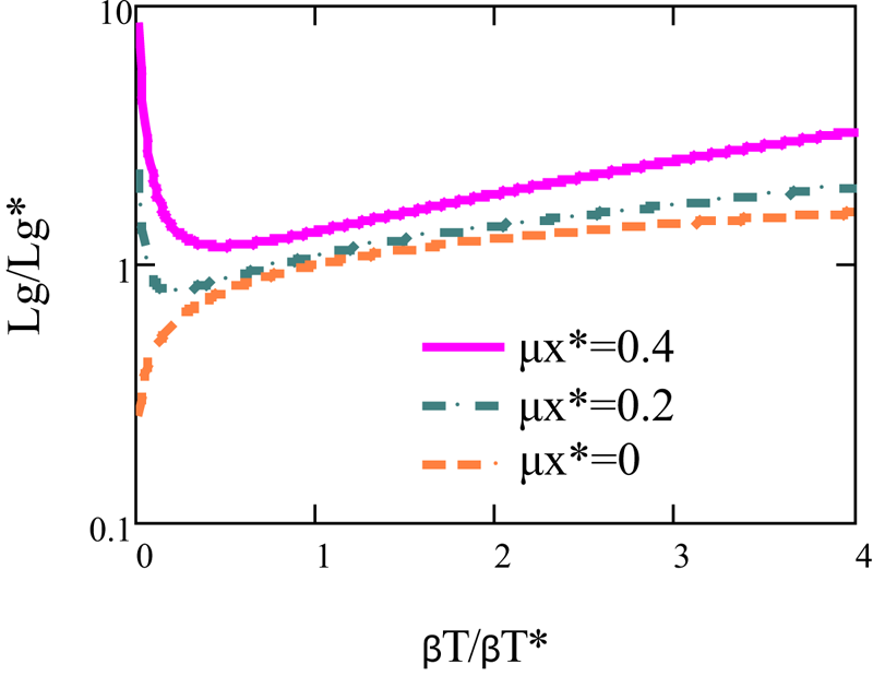
(2.15)\begin{equation} \left. \begin{gathered} {L_{g}=L_{g}^{*}X^{{1}/{3}}\left(1+\tilde{\mu}_{x}^{*2}X^{-{4}/{3}}\right)\left(1+\tilde{\mu}_{x}^{*2}X^{{4}/{3}}\right),}\\ {X=\frac{\beta_{T}}{\beta_{T}^{*}}}, \end{gathered} \right\} \end{equation}

where $L_{g}^{*}={\lambda _{u}}/{4{\rm \pi} \sqrt {3}\rho^{\ast}}$ is the gain length evaluated in the condition of natural focusing of the undulator (see (2.4a,b) and (2.6)). The expression in (2.15) is plotted in figure 1.

Figure 1.

Gain length as a function of the Twiss $\beta$ parameter, from (2.15). Both quantities are given in terms of their counterparts evaluated for the case of natural focusing for the undulator (indicated with the star symbol). For this reason, the ratio $L/L_{g}^{*}$ is plotted (on a logarithmic scale) as a function of the ratio $\beta _{T}/\beta _{T}^{*}$ in the case with null $\alpha _{T}$ Twiss matching parameter, for different values of $\tilde {\mu }_{x}^{*}$. The case $\tilde {\mu }_{x}^{*}=0$ corresponds to a null emittance (see (2.9)), hence to no inhomogeneous broadening effects.

Here $\tilde {\mu }_{x}^{*}=0$, corresponding to a null emittance (see (2.9)), which gives the case in the absence of any inhomogeneous broadening effects.

The evolution of the FEL power can be expressed in terms of a function of logistic nature

(2.16)\begin{equation} \left. \begin{gathered} {P\left(z\right)=P_{0}\frac{A\left(z\right)}{1+\dfrac{P_{0}}{P_{F}}\left[A\left(z\right)-1\right]}},\\ {A\left(z\right)=\frac{1}{9}\left[3+2\cosh\left(\frac{z}{L_{g}}\right)+4\cos\left(\frac{\sqrt{3}}{2}\frac{z}{L_{g}}\right)\cosh\left(\frac{z}{2L_{g}}\right)\right]}, \end{gathered} \right\} \end{equation}

where $P_{F}=\sqrt {2}\rho P_{E}$ is the FEL saturation power and $P_{E}$ is the electron beam energy. The gain length $L_g$ contains the effect of the non-ideal beam qualities determining the increase of the saturation length.

3. Emittance and collective effects

A further element of complexity is provided by the role played by slice and projected emittances. The distinction arises when the slippage length (namely the mismatch between laser and electrons due to the different velocities) is significantly shorter than the bunch length.

The FEL coherence length $l_{c}$ is defined by the identity

(3.1)\begin{equation} l_{c}\simeq\frac{\lambda}{4{\rm \pi}\sqrt{3}\rho} \end{equation}

where $\lambda$ is the resonance wavelength of the FEL radiation (2.8). The same quantity can be exploited to define the slippage, for undulators with $\rho \simeq 1/N$.

In the literature, different definitions of $l_{c}$ can be found, being limited to numerical constants but they do not produce any significant deviations regarding the physical consequences. The number of slices is approximately fixed by the ratio of the bunch length to the slippage/coherence length, namely

(3.2)\begin{equation} m\simeq\frac{\sigma_{z}}{l_{c}}. \end{equation}

The slices grows almost independently, each of them is characterized by its own phase space, emittance and energy spread. Here we use the coasting beam approximation and assume that each slice has identical phase space distribution, emittance and energy spread.

The projected beam qualities are all referred to the whole bunch. Projected and slice phase spaces are characterized by different dynamics. The collective effects, as coherent synchrotron radiation (CSR) and geometric transverse wakefield (GTW), may create misalignments increasing the projected emittance and leaving unaltered the slice counterparts (Di Mitri & Spampinati Reference Di Mitri and Spampinati2014). In other words, the projected emittance is expected to be larger than the slice emittance.

The point we would like to raise is how to account for the detrimental effects induced on the FEL dynamics by the increase of the projected emittance using the criteria developed in the previous picture.

Previous papers have addressed this problem. In particular, in Dattoli et al. (Reference Dattoli, Sabia, Ronsivalle, Del Franco and Petralia2012b) it has been afforded by defining the projected emittance by including the different phase space distributions of the individual slices and calculating the emittance growth including the statistical effects deriving from the Twiss coefficients characterizing the individual slices.

In Di Mitri & Spampinati (Reference Di Mitri and Spampinati2014) a different analysis has been performed and it has been shown that a $\tilde {\mu }$-like parameter can be defined and the increase of gain length due to the induced growth of the projected emittance can be naturally included by embedding it within a procedure similar to that discussed so far.

We have already noted that emittance contributes to the bunching smearing through the (incoherent) contributions due the angular and spatial contents of the bunch distribution, the coherent (collective) contribution is associated with the rms divergence $\langle \vartheta ^{2}\rangle$ of the slice centroids inside the undulator. The dilution of the bunching due to this contribution may become even larger than that corresponding to the incoherent parts.

The reference parameter adopted in Di Mitri & Spampinati (Reference Di Mitri and Spampinati2014) is

(3.3)\begin{equation} \left. \begin{gathered} {\tilde{\mu}_{\textrm{coll}}=\frac{\left\langle \vartheta^{2}\right\rangle }{\vartheta_{0}^{2}},}\\ {\vartheta_{0}^{2}=\frac{\lambda}{L_{g}}}, \end{gathered} \right\} \end{equation}

where the subscript ‘coll’ stands for ‘collective’. The critical angle $\vartheta _{0}$, in terms of the FEL characteristic quantities, can be written as

(3.4)\begin{equation} \vartheta_{0}^{2}=\frac{\lambda}{L_{g}}=\frac{2{\rm \pi}\sqrt{3}\rho}{\gamma^{2}}\left(1+\dfrac{K^{2}}{2}\right). \end{equation}

Thus, we obtain

(3.5)\begin{equation} \tilde{\mu}_{\textrm{coll}}=\frac{\gamma^{2}\left\langle \vartheta^{2}\right\rangle }{\left(1+\dfrac{K^{2}}{2}\right)2{\rm \pi}\sqrt{3}\rho}. \end{equation}

The analogy with $\tilde {\mu }_{x'}$ is evident. If we interpret ${\varepsilon }/{\beta _{T}}=\langle x'^{2}\rangle$ as beam divergence we can write $\tilde {\mu }_{x'}$ as

(3.6)\begin{equation} \tilde{\mu}_{x'}=\frac{\varepsilon}{\beta_{T}}\frac{\gamma^{2}}{\rho}\frac{1}{\left(1+\dfrac{K^{2}}{2}\right)}=\frac{\gamma^{2}\left\langle x'^{2}\right\rangle }{\rho\left(1+\dfrac{K^{2}}{2}\right)}=2{\rm \pi}\sqrt{3}\frac{\left\langle x'^{2}\right\rangle }{\vartheta_{0}^{2}}. \end{equation}

The physical nature of $\tilde {\mu }_{\textrm {coll}}$ can therefore be considered not extraneous to the previously outlined formalism.

In Di Mitri & Spampinati (Reference Di Mitri and Spampinati2014) it has been proposed and checked, by comparison with computer simulation, that such an inclusion occurs through the following re-definition of the $\chi$ function

(3.7)\begin{equation} L_{g,\textrm{coll}}=\frac{\chi}{1-\varsigma\,\tilde{\mu}_{\textrm{coll}}\chi}L_{g} \end{equation}

which we comment on in the following (if $\zeta ={\rm \pi}$ the previous equation reduces to the Tanaka formula derived in Tanaka et al. (Reference Tanaka, Kitamura and Shintake2004)).

The previous correction holds for the saturation length associated with detrimental effects due to slice tilting inside the electron bunch and eventually to the increase of the emittance to the projected value

(3.8)\begin{equation} \varepsilon_{\textrm{coll}}=\varepsilon\sqrt{\left|\begin{array}{cc} {\beta_{T}} & {-\alpha_{T}}\\ {-\alpha_{T}} & {\gamma_{T}+\dfrac{\left\langle x_{\textrm{coll}}'^{2}\right\rangle }{\varepsilon}} \end{array}\right|} \end{equation}

with the $\gamma _{T}$ Twiss coefficient modified by the inclusion of the slice centroid-associated divergence. Assuming $\alpha _{T}=0$, we express the emittance growth due to collective effects as

(3.9)\begin{equation} \varepsilon_{\textrm{coll}}=\varepsilon\sqrt{1+\frac{\beta_{T}\left\langle x_{\textrm{coll}}'^{2}\right\rangle }{\varepsilon}} \end{equation}

and, hence, the normalized collective (projected) emittance $\epsilon _{n,\textrm {coll}}=\gamma \epsilon _{\textrm {coll}}$.

The previous identity becomes a measure of $\langle x'^{2}\rangle$ through the evaluation of the projected emittance. We set

(3.10)\begin{equation} \left. \begin{gathered} \left\langle x'^{2}\right\rangle =\varDelta\frac{\epsilon}{\beta_{T}},\\ \varDelta=\left(\frac{\epsilon_{\textrm{coll}}}{\epsilon}\right)^{2}-1, \end{gathered} \right\} \end{equation}

and write $\tilde {\mu }_{\textrm {coll}}$ as

(3.11)\begin{equation} \tilde{\mu}_{\textrm{coll}}=\frac{\varDelta}{\beta_{T}}\frac{\lambda_{u}}{4{\rm \pi}\sqrt{3}\rho}\frac{\epsilon}{\lambda}. \end{equation}

According to the previous identity, large beta values should smear out the detrimental effect of the collective tilt.

The use of the parameter $X$, introduced in (2.15), allows to cast (3.11) in the more convenient form

(3.12)\begin{equation} \tilde{\mu}_{\textrm{coll}}=\frac{\varDelta}{\beta_{T}^{*}}\frac{\lambda_{u}}{4{\rm \pi}\sqrt{3}\rho^{*}X^{2/3}}\frac{\epsilon}{\lambda}. \end{equation}

The correction to the saturation length foreseen in (3.7), predicts a critical value of $\beta _{T}$ for which the collective effects are dominating over those associated with those due to the inhomogeneous broadening. This critical value occurs when, in (3.7), $\tilde {\mu }_{\textrm {coll}}=\zeta ^{-1}$, namely when

(3.13)\begin{equation} \beta_{\textrm{ct}}=\left[\frac{\varDelta}{\zeta\beta_{T}^{*}}L_{g}^{*}\frac{\epsilon}{\lambda}\right]^{3/2}\beta_{T}^{*} \end{equation}

obtained by assuming negligible inhomogeneous effects due to emittance, choosing ${\epsilon }/{\lambda }={1}/{4{\rm \pi} }$ eventually yields

(3.14)\begin{equation} \beta_{\textrm{ct}}=\left[\frac{\varDelta}{4{\rm \pi}\zeta\beta_{T}^{*}}L_{g}^{*}\right]^{3/2}\beta_{T}^{*}. \end{equation}

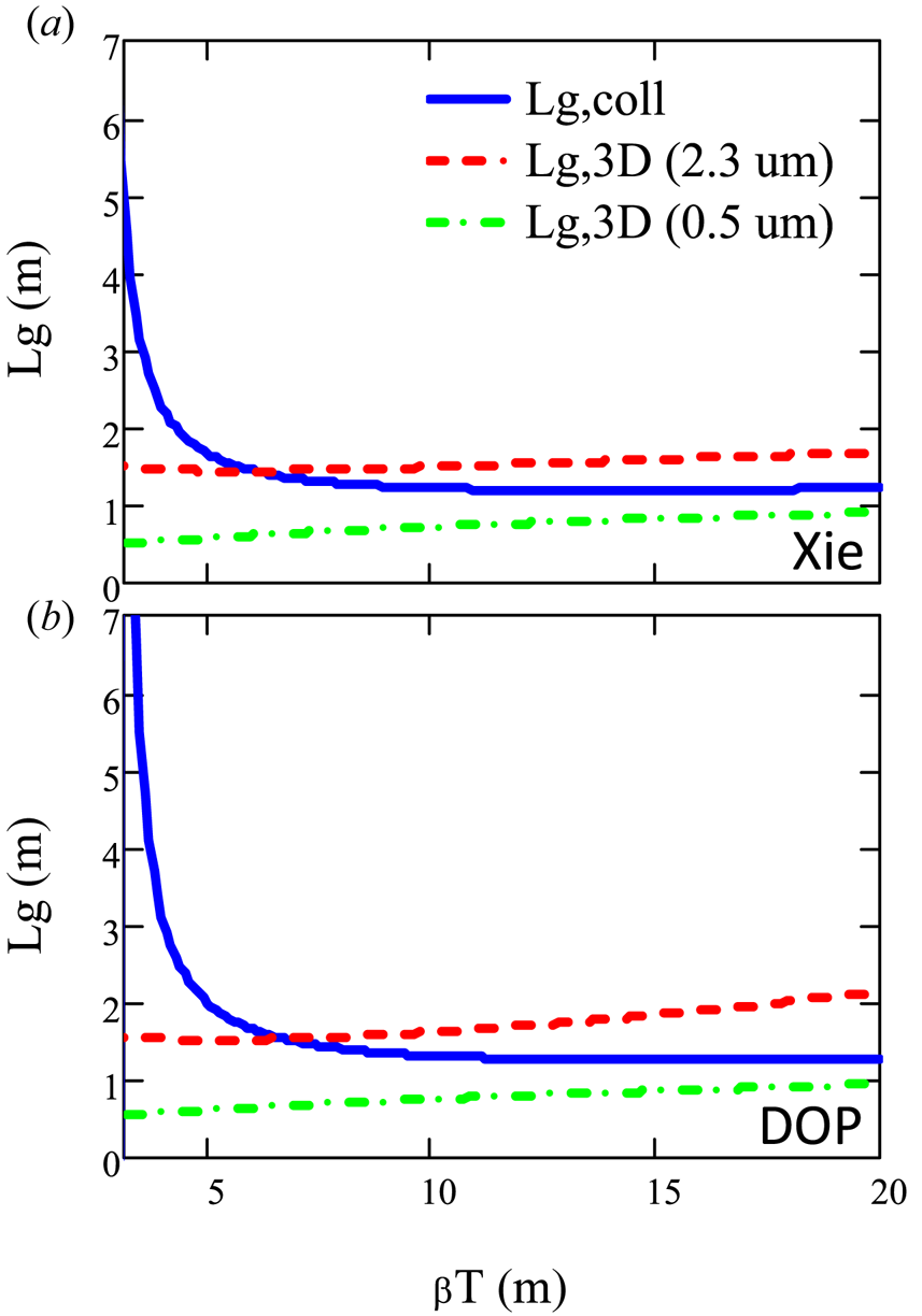
In correspondence to this value, the saturation length becomes prohibitively long, at least according to the assumption that $\tilde {\mu }_{\textrm {coll}}$ induced effects are accounted for by an equation of the type (3.7). 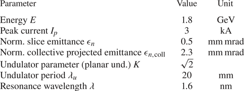In figure 2 we have compared the saturation length versus $\beta _{T}$ for the cases corresponding to a normalized slice emittance $\epsilon _{n}$, a normalized projected emittance $\epsilon _{n,\textrm {coll}}$ and to the collective effect with parameters of table 1 for the electron beam and radiation. Very similar results are obtained by using the Xie (also used in Di Mitri & Spampinati Reference Di Mitri and Spampinati2014) or the DOP formalism to evaluate the three-dimensional corrections to the gain length. The plot axes are limited to a minimum considered $\beta _{T,{\rm min}}=3$ because (with the assumed parameters for the electron beam) a singularity occurs, owing to the form of (3.7), for lower $\beta _{T}$ values where the equation is supposed to have no more physical sense. It is worth noting that when $\beta _{T}\gg \beta _{\textrm {ct}}$, the saturation length retains reasonable values, in between those associated with slice and collective emittance.

Figure 2.

Gain length, calculated with the parameters listed in table 1, as a function of the average Twiss $\beta$ parameter in the undulator according to (3.7). In $(a)$, $L_{g,3D}$ has been evaluated according to the Xie formalism according to results in Di Mitri & Spampinati (Reference Di Mitri and Spampinati2014); in $(b)$, the DOP model, used in the present paper, has been considered to evaluate the inhomogeneous broadening effects on the gain length. Dashed green and dotted red lines refer to situations when no misalignment is present: in these cases, the projected emittance coincides with the slice emittance and $L_{g,\textrm {coll}}$ reduces to $L_{g,3D}$, the two lines are obtained for $\epsilon _{n}=0.5\ \textrm {mm}\,\textrm {mrad}$ and $\epsilon _{n}=2.3\ \textrm {mm}\,\textrm {mrad}$, respectively. The blue continuous line refers to $L_{g,\textrm {coll}}$ in the presence of a misalignment where the norm. slice emittance $\epsilon _{n}=0.5\ \textrm {mm}\,\textrm {mrad}$ and the norm.projected value is $\epsilon _{n,\textrm {coll}}=2.3\ \textrm {mm}\,\textrm {mrad}$. In all cases the effects of the energy spread have not been considered ($\tilde {\mu }_{\epsilon }=0)$. It is evident that for small $\beta _{T}$ values, an increase of the gain length occurs, where this condition is of course inauspicious for FEL operation.

Table 1.

Set of parameters used to compare the gain length modified by collective effects with $L_{g,3D}$, as a function of the Twiss $\beta$ parameter. The slice emittance is supposed to be the same for all slices. Projected emittance coincides with the projected emittance if no misalignment of the slices occurs in the phase space.

4. An alternative point of view

The contribution of the collective effects, using (3.7), appears as a separate function, appended to the inhomogeneous $\chi$ function and without affecting the other quantities entering the definition of the other $\tilde {\mu }$ parameters.

A different way of looking at the increasing gain length caused by the collective effects is to leave the same expression as in (2.14), but replacing $\varepsilon$ with $\varepsilon _{\textrm {coll}}$ wherever the emittance appears.

Regarding the Pierce parameter and the fact that it is proportional to the cubic root of the beam current density, the correction due to the ‘collective’ emittance yields

(4.1)\begin{equation} \left. \begin{gathered} {\rho_{\textrm{coll}}=\rho\left(\frac{\sigma}{\sigma_{\textrm{coll}}}\right)^{{2}/{3}}=\rho\left(\frac{\epsilon}{\epsilon_{\textrm{coll}}}\right)^{{1}/{3}},}\\ {\sigma_{\textrm{coll}}=\sqrt{\beta_{T}\varepsilon_{\textrm{coll}}}}. \end{gathered} \right\} \end{equation}

As to the inhomogeneous broadening, we end up with

(4.2)\begin{equation} \left. \begin{gathered} {\tilde{\mu}_{x',\textrm{coll}}=\frac{\varepsilon_{\textrm{coll}}}{\beta_{T}}\frac{\gamma^{2}}{\rho_{\textrm{coll}}}\frac{1}{\left(1+\dfrac{K^{2}}{2}\right)},}\\ {\tilde{\mu}_{x,\textrm{coll}}=\varepsilon_{\textrm{coll}}\frac{\gamma^{2}}{\rho_{\textrm{coll}}}\frac{1}{\left(1+\dfrac{K^{2}}{2}\right)}\frac{\left(\gamma_{T}^{*}\right)^{2}}{\gamma_{T}},}\\ {\tilde{\mu}_{\varepsilon,\textrm{coll}}=\frac{2\sigma_{\varepsilon}}{\rho_{\textrm{coll}}}}. \end{gathered} \right\} \end{equation}

It is more convenient to cast them in the form

(4.3)\begin{equation} \left. \begin{gathered} {\tilde{\mu}_{x',\textrm{coll}}=\tilde{\mu}_{x'}\left(\frac{\varepsilon_{\textrm{coll}}}{\varepsilon}\right)^{{5}/{3}},}\\ {\tilde{\mu}_{x,\textrm{coll}}=\tilde{\mu}_{x}\left(\frac{\varepsilon_{\textrm{coll}}}{\varepsilon}\right)^{{5}/{3}}},\\ {\tilde{\mu}_{\varepsilon,\textrm{coll}}=\tilde{\mu}_{\varepsilon}\left(\frac{\varepsilon_{\textrm{coll}}}{\varepsilon}\right)^{{1}/{3}}}, \end{gathered} \right\} \end{equation}

which shows that the correction associated with slice misalignment can be characterized by the ratio $\varepsilon _{\textrm {coll}}/\varepsilon$.

With these redefinitions of the $\tilde {\mu }$ parameters, the $\chi$ function of (2.14) can be rewritten in order to achieve a corrected albeit approximate expression that includes the collective effects. We can write the function of the $\rho$ depleting formula, and hence the gain length as

(4.4)\begin{equation} \frac{L_{g}^{(\textrm{coll})}}{L_{g}}=\chi_{\textrm{coll}}\simeq1+\left(\frac{\varepsilon_{\textrm{coll}}}{\varepsilon}\right)^{{2}/{3}}\left[\left(\tilde{\mu}_{x}^{2}+\tilde{\mu}_{x'}^{2}\right)\left(\frac{\varepsilon_{\textrm{coll}}}{\varepsilon}\right)^{{8}/{3}}+d\tilde{\mu}_{\varepsilon}^{2}\right] \end{equation}

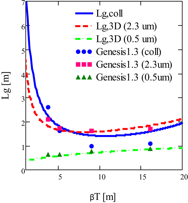
obtained by neglecting the cross products, where it is also evident the increase of the gain length (hence, of the saturation length) at low $\beta _{T}$ values. Equation (4.4) has been plotted in figure 3 and compared with a set of numerical simulations, already shown in Di Mitri & Spampinati (Reference Di Mitri and Spampinati2014) and made with the code GENESIS 1.3 (Reiche Reference Reiche1999), with good agreement especially for $\beta _{T}$ values in the reasonable range of operation for an actual FEL with the parameters in table 1.

Figure 3.

Gain length with the inclusion of the collective effects evaluated from (4.4). Dashed green and dotted red lines refer to situations when no misalignment is present and for $\epsilon _{n}=0.5\ \textrm {mm}\,\textrm {mrad}$ and $\epsilon _{n}=2.3\ \textrm {mm}\,\textrm {mrad}$, respectively. The blue continuous line is the gain length $L_{g}^{(\textrm {coll})}$ with the inclusion of collective effects with a norm. slice emittance $\epsilon _{n}=0.5\ \textrm {mm}\,\textrm {mrad}$ and a norm. projected value $\epsilon _{n,\textrm {coll}}=2.3\ \textrm {mm}\,\textrm {mrad}$. Energy spread effects are not accounted ($\tilde {\mu }_{\epsilon }=0)$. The formula fits well with a set of GENESIS 1.3 numerical simulations, described in Di Mitri & Spampinati (Reference Di Mitri and Spampinati2014), especially in the region around the minimum $\beta _{T}$ in the optimum range of operation for an FEL with the parameters of table 1.

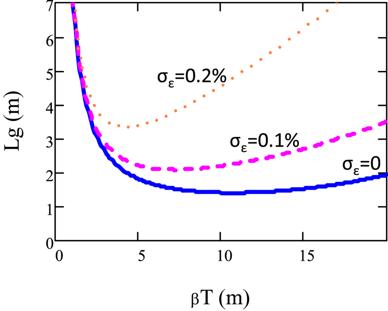
In figure 4 we have plotted the gain length $L_{g}^{(\textrm {coll})}$ ((4.4)) versus the Twiss parameter beta with also including the effect of the energy spread. The results show that the optimum $\beta _{T}$ value depends on the beam qualities. It is worth stressing that in the presence of a larger energy spread the optimization procedure may become critical.

Figure 4.

Gain length $L_{g}^{(\textrm {coll})}$ calculated with the parameters listed in table 1, as a function of the average Twiss $\beta _{T}$ parameter in the undulator, with the inclusion of the effects due to energy spread $\sigma _{\epsilon }=2\rho \tilde {\mu }_{\epsilon }$. Different lines have been calculated, with a norm.slice emittance $\epsilon _{n}=0.5\ \textrm {mm}\,\textrm {mrad}$ and a norm. collective projected emittance $\epsilon _{n,\textrm {coll}}=2.3\ \textrm {mm}\,\textrm {mrad}$, for different values of the energy spread. Blue continuous, dashed purple and dotted orange lines are for $\sigma _{\epsilon }=0$, $\sigma _{\epsilon }=0.1\,\%$ and $\sigma _{\epsilon }=0.2\,\%$, respectively. It is evident, as expected, a deterioration of the beam, and hence an increase of the gain length, with higher energy spread values.

5. Final comments

The problem of the effect of slice phase space content on the FEL performances is a byproduct of the peculiar nature of the FEL interaction itself, in which the slippage plays a central role. Within this context it has been argued that beam transport is a problem concerning either the global (projected phase space) or the individual slice, whose longitudinal extension is fixed by the slippage length itself.

In this paper, we have addressed the problem of including the increase of the projected emittance growth due to slice misalignment, in the evaluation of the SASE FEL gain, thus determining the relevant detrimental effects on the saturation length. The key element of the analysis is the introduction of an inhomogeneous broadening-like parameter (Di Mitri & Spampinati Reference Di Mitri and Spampinati2014) that measures the increase of emittance due to collective effects. In order to preserve a line of continuity with the treatment in Xie (Reference Xie1995) and Saldin et al. (Reference Saldin, Schneidmiller and Yurkov2004) it is assumed that this effect is not a separated function and affects the saturation length through a suitable redefinition of the Pierce parameter. An effective idea of the interplay between the various detrimental contributions to the increase of the saturation length is offered by the approximate expression of the $\chi$ function given in (4.4), which yields an idea of how the various terms due to collective, slice emittances and energy spread contribute to the increase of the gain length. Both models indicate that a strong deterioration of the gain length occurs at low values of the matching $\beta _{T}$ Twiss parameter, thus making the FEL operation critical. The use of (4.4) avoids the singularity given by the form of (3.7). Both parametrizations give good agreement with numerical simulations. The choice of one or the other is matter of a careful analysis of the experimental results.

It should be noted that in an actual FEL the optimization of the Twiss $\beta$ function is limited by the length of the so-called FODO cell (Holzer Reference Holzer2013), the magnetic structure consisting alternately of focusing and defocusing elements (quadrupoles), and by the maximum achievable quadrupole strength. A typical FODO length is 5–8 m for a soft X-ray FEL (with electron beam energy up to 5 GeV) and the average beta value can be reasonably optimized in the range 5–15 m.

Until now the most frequently adopted optimization procedure in FELs is a beam-based alignment (BBA) where the quadrupoles of the FODO lattice are tuned one by one in order to maximize the output FEL pulse energy at each step. The inconvenience is that the BBA procedure must be restarted each time the machine setup has to be changed. Different strategies may be adopted to define an appropriate beam transport when the slice dynamics is important (see Dattoli et al. Reference Dattoli, Sabia, Del Franco and Petralia2012a; Lazzarino et al. Reference Lazzarino, Di Palma, Anania, Artioli, Bacci, Bellaveglia, Chiadroni, Cianchi, Ciocci and Dattoli2014). In particular, it is important to define suitable experiments to investigate the effect of the beam transport itself on the evolution of the projected quantities. These types of benchmarking experiments give confidence in the model underlying the theory and make the optimization criteria developed so far more reliable.

Before concluding, we would like to address a further important, sometimes ignored problem, regarding the space charge gain detrimental contribution, which can determine sizeable effects in high-energy high-current X-ray FEL devices. This effect can be quantified by means of the corresponding parameter (Dattoli, Fares & Licciardi Reference Dattoli, Fares and Licciardi2020):

(5.1)\begin{equation} \tilde{\mu}_Q=\frac{{5 \times 10^{-6}}}{{\gamma\rho}}\left[\frac{{E_f}}{{E_e}}\frac{{\dot{N}_e\lambda^2_u}}{{\beta_T}}\right]^{1/2}. \end{equation}

Keeping, for example, $E_e=15\ \textrm {GeV}$, $E_f=12.4\ \textrm {keV}$, $\lambda _u=0.04\ \textrm {m}$, $\beta _T=8\ \textrm {m}$ and assuming $\gamma \rho =5$, we obtain $I>5\ \textrm {kA}$.

Non-negligible effects on the saturation length can be observed (for further comments, see Dattoli et al. (Reference Dattoli, Fares and Licciardi2020) and references therein for earlier papers on this subject). Slices may carry different amounts of charges, hence the effect of space charge dilution is a further distinctive feature within their dynamics. This aspect of the problem will be carefully treated elsewhere.

Editor William Dorland thanks the referees for their advice in evaluating this article.