1. Introduction
The equations for ideal fluid motion can be expressed in Hamiltonian form with non-canonical Poisson brackets (Morrison & Greene Reference Morrison and Greene1980; Morrison Reference Morrison1998). Non-canonical Hamiltonian systems generally have Casimir invariants which Poisson-commute with arbitrary functionals. The Casimir invariants play an important role in understanding the dynamics of the system. In fact, the system evolves in time on a Casimir leaf, which is specified by the values of the Casimir invariants. On the Casimir leaf, the system evolves along a contour of the Hamiltonian since the Hamiltonian is a conserved quantity. An extremum of the Hamiltonian corresponds to a stationary state of the system on the Casimir leaf (Arnol’d Reference Arnol’d1965; Holm et al. Reference Holm, Marsden, Ratiu and Weinstein1985).
A vorticity equation for an incompressible, ideal neutral fluid in two dimensions is one such Hamiltonian system. Let us assume that the boundary of the domain is periodic in both dimensions. Then the energy, as well as the Casimir invariants such as enstrophy, is conserved. Since the vorticity is only convected by the corresponding velocity field in the two-dimensional plane, the area integral of any function of the vorticity does not change during the time evolution. The area integral is the Casimir invariant. Suppose that the velocity field for the convection is changed to another one which is not directly related to the vorticity field. Even in this case, the vorticity is still only convected in the two-dimensional plane. Thus the Casimir invariants of the original system remain as invariants. However, the dynamics is artificial now and thus the energy of the system can change. Thus, if we can prepare an artificial velocity field that causes the energy to change monotonically, we may reach a stationary state on the original Casimir leaf. This method was first proposed by introducing a modified convection velocity field for the Euler equation (Vallis, Carnevale & Young Reference Vallis, Carnevale and Young1989). By the modified dynamics, it was shown that the energy can increase or decrease monotonically while preserving the Casimir invariants of the original Euler equation, reaching the extremum of the energy. Numerical simulation results were further shown to demonstrate the feasibility of the method of modified dynamics (Carnevale & Vallis Reference Carnevale and Vallis1990). The method of modified dynamics was then extended to general Hamiltonian dynamical systems (Shepherd Reference Shepherd1990). Furthermore, this method was extended by introducing Dirac brackets and symmetric brackets (Flierl & Morrison Reference Flierl and Morrison2012). The former imposes additional conserved quantities such as angular momentum; thus we may be able to obtain a variety of stationary states. The latter can introduce a kind of filter; for example, high-wavenumber structures tend to be suppressed. In Flierl & Morrison (Reference Flierl and Morrison2012), numerical simulation results using these brackets were described for two-dimensional vortex dynamics. Here, any method that modifies the original dynamics while leaving the Casimir invariants unchanged will be called a simulated annealing (SA) method.
One of the advantages of the SA method is that the stationary states are characterized by the Casimir invariants. Since the stationary state is an extremum of the Hamiltonian on a Casimir leaf, it is natural to characterize stationary states by the Casimir invariants from the theoretical point of view. On the other hand, the values of the Casimir invariants are fully determined by the initial condition for the SA method, since they are kept unchanged during the modified dynamics of the SA method. Therefore, if we try to characterize the stationary states by the values of the Casimir invariants, it might be better to have a method to prepare an appropriate initial condition which has the desired values of the Casimir invariants. This is our motivation in the present paper: we will develop a method to adjust an initial condition for SA to have the desired values of the Casimir invariants, and then we can systematically classify the stationary states. Moreover, as shown below, we can obtain a non-trivial stationary state by controlling a value of a Casimir invariant for low-beta reduced magnetohydrodynamics (MHD) (Strauss Reference Strauss1976; Hazeltine & Meiss Reference Hazeltine and Meiss2003) in two dimensions, which is also a non-canonical Hamiltonian system. Here beta denotes a ratio of the plasma pressure to the magnetic pressure.
Here we make two remarks regarding the motivation. The first strengthens our motivation. We know that a two-dimensional stationary state is easily obtained by solving the Poisson equation
 ${\rm\Delta}{\it\varphi}={\it\omega}({\it\varphi})$
by assuming a function
 ${\it\omega}({\it\varphi})$
. Here, the fluid velocity in the two-dimensional plane, say the
 $x{-}y$
plane, is given by
 $\boldsymbol{v}=\hat{\boldsymbol{z}}\times \boldsymbol{{\rm\nabla}}{\it\varphi}$
, where
 ${\it\varphi}$
and
 $\hat{\boldsymbol{z}}$
, respectively, are a stream function and a unit vector perpendicular to the
 $x{-}y$
plane. Moreover,
 ${\rm\Delta}:=\partial ^{2}/\partial x^{2}+\partial ^{2}/\partial y^{2}$
denotes the two-dimensional Laplacian. Then
 ${\it\omega}:=\hat{\boldsymbol{z}}\boldsymbol{\cdot }\boldsymbol{{\rm\nabla}}\times \boldsymbol{v}$
is the vorticity. The stationary state is characterized by the functional form of
 ${\it\omega}({\it\varphi})$
. Even in this case, we may be able to systematically classify the stationary state by introducing some parameters such as
 $c$
and
 ${\it\alpha}$
to express
 ${\it\omega}$
as
 ${\it\omega}({\it\varphi})=c{\it\varphi}^{{\it\alpha}}$
, for example. However, the obtained series of stationary states may have different values for the Casimir invariants. The situation is the same for low-beta reduced MHD in two dimensions. Conventionally we obtain stationary states by solving an elliptic equation, the so-called Grad–Shafranov (G–S) equation (Grad & Rubin Reference Grad and Rubin1958; Shafranov Reference Shafranov1958). Therefore, it would be better to have another method to obtain a series of stationary states with values of the Casimir invariants being varied in a systematic way.
The second remark arises from the two-dimensionality. The stationary state of an incompressible, ideal neutral fluid, as well as low-beta reduced MHD in two dimensions, has an infinite number of Casimir invariants. Even if we try to adjust the initial conditions for SA as much as possible, the number of Casimir invariants so specified does not exceed the number of grids or mode expansions in the numerical computation. We cannot adjust the initial condition completely in the two-dimensional problem. As we will show below, we develop a method to specify a finite number of Casimir invariants. Thus the application of this method to two-dimensional problems does not seem to have any advantage compared to the Poisson equation method. However, the point is that the developed method is not restricted to two dimensions: it also applies to three dimensions. If we achieve a reliable method to specify values for a finite number of Casimir invariants, it should be critical for three-dimensional problems since we can completely characterize the stationary states by those Casimir invariants.
This paper is organized as follows. In § 2 we first give a brief introduction to the SA method for an incompressible, ideal neutral fluid in two dimensions as the simplest example. The Hamiltonian form of the system is also explained. Then we develop the method to adjust the vorticity field so that it has specified values for a finite number of Casimir invariants. In § 3 we demonstrate that our method succeeds in adjusting the vorticity field to have desired values for the Casimir invariants. Then, in § 4, we apply the SA method with the adjusted vorticity field as an initial condition. An example is shown to demonstrate that we obtain a stationary state of the system with the specified values of the Casimir invariants. In § 5 we apply the method to low-beta reduced MHD in two dimensions. By specifying the value of the cross-helicity, we obtain a non-trivial stationary state, which may be difficult to obtain by solving the G–S equation. Concluding remarks are given in § 6.
2. Theory
2.1. Brief review of the SA method
The vorticity equation for an incompressible, ideal neutral fluid in two dimensions is given by
 $$\begin{eqnarray}\frac{\partial {\it\omega}}{\partial t}=[{\it\omega},{\it\varphi}].\end{eqnarray}$$
Here we consider that the fluid motion occurs in the
 $x{-}y$
plane, and the fluid velocity
 $\boldsymbol{v}(x,y)$
is given as
 $\boldsymbol{v}=\hat{\boldsymbol{z}}\times \boldsymbol{{\rm\nabla}}{\it\varphi}$
, where
 ${\it\varphi}(x,y)$
is the stream function and
 $\hat{\boldsymbol{z}}$
is a unit vector perpendicular to the
 $x{-}y$
plane. The vorticity is defined by
 ${\it\omega}:={\rm\Delta}{\it\varphi}$
, where
 ${\rm\Delta}:=\partial ^{2}/\partial x^{2}+\partial ^{2}/\partial y^{2}$
is a two-dimensional Laplacian. The Poisson bracket is defined by
 $[f,g]:=(\partial f/\partial x)(\partial g/\partial y)-(\partial f/\partial y)(\partial g/\partial x)$
for arbitrary functions
 $f$
and
 $g$
. A stationary state of the system is characterized by the functional form
 ${\it\omega}({\it\varphi})$
.
A general Hamiltonian system is given by
 $$\begin{eqnarray}\frac{\partial u}{\partial t}=\mathscr{J}\frac{{\it\delta}H}{{\it\delta}u},\end{eqnarray}$$
where
 $u$
is a state vector,
 $H[u]$
is a Hamiltonian, which is a functional of
 $u$
, and
 $\mathscr{J}$
is an anti-symmetric operator. Here,
 ${\it\delta}H/{\it\delta}u$
denotes the functional derivative of
 $H$
with respect to
 $u$
. We see that the vorticity equation has this form by taking the scalar state
 $u={\it\omega}$
,
 $$\begin{eqnarray}\displaystyle H[{\it\omega}]=-\frac{1}{2}\int _{\mathscr{D}}{\it\omega}({\rm\Delta}^{-1}{\it\omega})\,\text{d}x\,\text{d}y, & & \displaystyle\end{eqnarray}$$
and
 $$\begin{eqnarray}\mathscr{J}=-[{\it\omega},\circ ].\end{eqnarray}$$
Here,
 $\boldsymbol{{\rm\nabla}}$
and
 $\mathscr{D}$
denote the gradient operator and the domain in the
 $x{-}y$
plane, respectively. Note that
 ${\rm\Delta}^{-1}{\it\omega}={\it\varphi}$
and thus
 $H$
gives the kinetic energy, and
 ${\it\delta}H/{\it\delta}{\it\omega}=-{\it\varphi}$
in the present case. A Casimir invariant is a functional
 $C$
that satisfies
 $\mathscr{J}({\it\delta}C/{\it\delta}u)\equiv 0$
, which is given by
 $$\begin{eqnarray}C[{\it\omega}]=\int _{\mathscr{D}}f({\it\omega})\,\text{d}x\,\text{d}y,\end{eqnarray}$$
where
 $f({\it\omega})$
is an arbitrary function of
 ${\it\omega}$
. Note that we implicitly assume that all functions are suitably differentiable. Here
 ${\it\delta}C/{\it\delta}{\it\omega}=\text{d}f({\it\omega})/\text{d}{\it\omega}$
, and we see that
 $\mathscr{J}({\it\delta}C/{\it\delta}{\it\omega})\equiv 0$
is satisfied. One of the examples is enstrophy, where
 $f({\it\omega})={\it\omega}^{2}/2$
. Since
 $f({\it\omega})$
is arbitrary, we have an infinite number of Casimir invariants in this system.
Note that a stationary state of this system is given by
 ${\it\delta}(H+C)/{\it\delta}{\it\omega}=0$
or equivalently
 ${\it\varphi}=\text{d}f({\it\omega})/\text{d}{\it\omega}$
. Therefore
 ${\it\varphi}$
becomes a function of
 ${\it\omega}$
at a stationary state.
Now, let us explain the SA method. Although a variety of modifications has been developed so far (Vallis et al. Reference Vallis, Carnevale and Young1989; Carnevale & Vallis Reference Carnevale and Vallis1990; Shepherd Reference Shepherd1990; Flierl & Morrison Reference Flierl and Morrison2012), in § 4 we adopt the modified dynamics
 $$\begin{eqnarray}\frac{\partial u}{\partial t}=-\mathscr{J}^{2}\frac{{\it\delta}H}{{\it\delta}u}.\end{eqnarray}$$
This may be the simplest one. By applying
 $\mathscr{J}$
twice, we can prove that
 $H$
changes monotonically while
 $C$
is preserved as an invariant. Thus we can reach an extremum of
 $H$
to obtain a stationary state by solving this modified dynamics by keeping
 $C$
unchanged in the original dynamics. The minus sign in front of
 $\mathscr{J}^{2}$
is to increase
 $H$
. The definitions of
 $u$
,
 $H[u]$
and
 $\mathscr{J}$
are as introduced above for the vorticity equation. In § 5 we apply the symmetric bracket developed in Flierl & Morrison (Reference Flierl and Morrison2012) to low-beta reduced MHD in two dimensions.
2.2. Adjustment of vorticity fields via the steepest descent method
Now let us explain how we adjust values of the Casimir invariants. Suppose we try to adjust values of Casimir invariants defined by
 $$\begin{eqnarray}C_{j}:=\int _{\mathscr{D}}f_{j}({\it\omega})\,\text{d}x\,\text{d}y,\quad j=j_{1},j_{2},\dots .\end{eqnarray}$$
Here, we assume that the
 $f_{j}({\it\omega})$
are differentiable, linearly independent functions. For example,
 $C_{j}$
becomes enstrophy if we take
 $f_{j}({\it\omega})={\it\omega}^{2}/2$
. We introduce the functional
 $$\begin{eqnarray}W:=\mathop{\sum }_{j}(C_{j}-c_{j})^{2},\end{eqnarray}$$
where
 $c_{j}$
is the desired value of
 $C_{j}$
. If we consider a derivative
 $W$
with respect to an artificial time
 ${\it\tau}$
, we have
 $$\begin{eqnarray}\frac{\text{d}W}{\text{d}{\it\tau}}=2\int _{\mathscr{D}}\left(\mathop{\sum }_{j}w_{j}\right)\frac{\partial {\it\omega}}{\partial {\it\tau}}\,\text{d}x\,\text{d}y,\end{eqnarray}$$
where
 $$\begin{eqnarray}w_{j}:=(C_{j}-c_{j})\frac{\text{d}f_{j}({\it\omega})}{\text{d}{\it\omega}}.\end{eqnarray}$$
Then, if we solve the equation
 $$\begin{eqnarray}\frac{\partial {\it\omega}}{\partial {\it\tau}}=-\mathop{\sum }_{j}w_{j},\end{eqnarray}$$
we obtain
 $$\begin{eqnarray}\frac{\text{d}W}{\text{d}{\it\tau}}=-2\int _{\mathscr{D}}\left(\mathop{\sum }_{j}w_{j}\right)^{2}\,\text{d}x\,\text{d}y\leqslant 0.\end{eqnarray}$$
Since
 $W$
is non-negative,
 $W$
reaches zero when
 $$\begin{eqnarray}\mathop{\sum }_{j}w_{j}=0\end{eqnarray}$$
is satisfied. Since
 $\text{d}f_{j}({\it\omega})/\text{d}{\it\omega}$
are independent,
 $C_{j}=c_{j}$
is obtained. This completes the adjustment of the values of the Casimir invariants. An extension to low-beta reduced MHD is straightforward.
Note that, formally, it seems that we can adjust arbitrarily many Casimir invariants. However, the number adjusted is actually limited by the number of grids or modes in the numerical computation. Further, note that the adjustment may become more difficult as we increase the number of Casimir invariants. Finally, note that the adjustment process is not restricted to two-dimensional systems: it can also be applied to three-dimensional systems.
3. Demonstration of the adjustment of a vorticity field
3.1. Adjustment of a vorticity field with desired values of the Casimir invariants
Let us first demonstrate that the method explained in the previous section actually works well. The arbitrary function determining the Casimir invariant is chosen as
 $f_{j}({\it\omega})={\it\omega}^{j}$
in the numerical results shown below. The domain
 $\mathscr{D}$
was chosen as a square region with
 $-{\rm\pi}\leqslant x<{\rm\pi}$
and
 $-{\rm\pi}\leqslant y<{\rm\pi}$
. Periodic boundary conditions were imposed in both
 $x$
and
 $y$
. Grid numbers are 128 in both
 $x$
and
 $y$
directions. A simple Euler scheme was adopted for the evolution in the artificial time. The time advancement was stopped when
 $|C_{j}-c_{j}|\leqslant 10^{-7}$
was satisfied for all
 $j$
. The vorticity field before adjusting the values of the Casimir invariants was
 ${\it\omega}=\cos x+\sin (y+\cos y)$
. This satisfies the periodic boundary condition but is not a stationary state of the vorticity equation. In the three cases shown below,
 $C_{2}=20$
was specified for all, and
 $C_{3}$
was specified to be different values. This means that we tried to obtain three kinds of initial conditions for SA that have different sets of the Casimir invariants. Note that the spatial average of
 ${\it\omega}$
of the pre-adjusted initial condition is not zero. However, it should be zero under doubly periodic boundary conditions. Therefore we also adjusted the vorticity field to be
 $C_{1}=0$
, together with the adjustment of
 $C_{2}$
and
 $C_{3}$
.







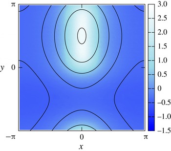
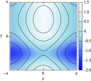
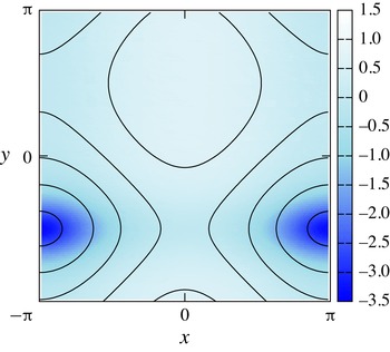
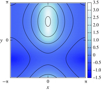
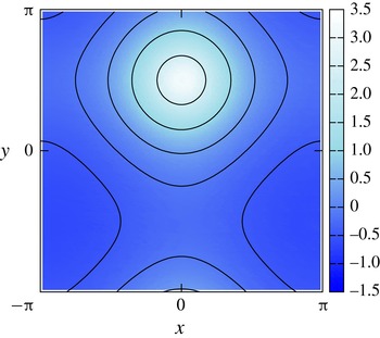
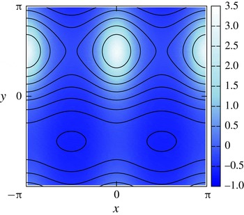
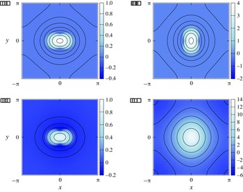
Figures 1–3 show the vorticity field after the adjustment, with contours of
 ${\it\varphi}$
and the colour map of
 ${\it\omega}$
in the
 $x{-}y$
plane. As noted above,
 $C_{1}=0$
and
 $C_{2}=20$
are the same for all cases. For figures 1–3,
 $C_{3}=30$
, 0 and
 $-30$
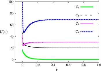
, respectively. Furthermore, the time histories of
 $C_{1}$
,
 $C_{2}$
,
 $C_{3}$
and
 $C_{4}$
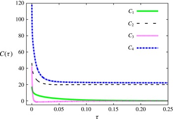
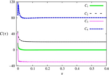
are shown in figures 4–6, respectively. We observe that
 $C_{1}$
,
 $C_{2}$
and
 $C_{3}$
converge to the specified values. In the case of figure 1,
 $C_{3}$
was set to a rather large positive value. Then the obtained vorticity field has a localized region with a large positive value of
 ${\it\omega}$
. Note that the colour representing
 ${\it\omega}=0$
is different in each figure. Similarly, the obtained vorticity field has a localized region with a large negative value of
 ${\it\omega}$
in the case of figure 3, where
 $C_{3}$
was set to a large negative value. This is because otherwise the specified value of
 $C_{3}$
cannot be realized together with the specified value of
 $C_{2}$
.




Time history of
 $C_{1}$
,
 $C_{2}$
,
 $C_{3}$
and
 $C_{4}$
is shown, corresponding to figure 1 with
 $C_{1}=0$
,
 $C_{2}=20$
and
 $C_{3}=30$
.

Time history of
 $C_{1}$
,
 $C_{2}$
,
 $C_{3}$
and
 $C_{4}$
is shown, corresponding to figure 2 with
 $C_{1}=0$
,
 $C_{2}=20$
and
 $C_{3}=0$
.

Time history of
 $C_{1}$
,
 $C_{2}$
,
 $C_{3}$
and
 $C_{4}$
is shown, corresponding to figure 3 with
 $C_{1}=0$
,
 $C_{2}=20$
and
 $C_{3}=-30$
.

Note that all other, unspecified Casimir invariants have different values: for example,
 $C_{4}=69.13$
, 22.10 and 80.37 for the vorticity field of figures 1–3, respectively. These unspecified
 $C_{j}$
depend on the vorticity field before adjustment as well as during the adjustment process, or during the evolution by (2.11) based on the steepest descent method, since (2.11) does not preserve values of
 $C_{j}$
.
We performed one more example of this kind:
 $C_{4}=80$
was also specified as well as
 $C_{1}=0$
,
 $C_{2}=20$
and
 $C_{3}=30$
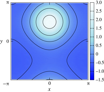
. The contours of
 ${\it\varphi}$
and the colour map of
 ${\it\omega}$
of the adjusted initial condition are shown in figure 7. This was also successful. As noted above, we cannot specify all the Casimir invariants since there exists an infinite number of Casimir invariants in two-dimensional systems. However, we demonstrated that our method adjusted several Casimir invariants, which could be critical in three-dimensional systems.
Adjusted vorticity field with
 $C_{4}=80$
as well as
 $C_{1}=0$
,
 $C_{2}=20$
,
 $C_{3}=30$
. The solid curves are contours of
 ${\it\varphi}$
, and the colour map shows
 ${\it\omega}$
. The pre-adjusted vorticity field was
 ${\it\omega}=\cos x+\sin (y+\cos y)$
, which is the same as those of figures 1–3.

We should remark that there are constraints on the Casimir invariants. As a simple example, it is obvious that we cannot specify negative
 $C_{2}$
. Similarly, if we specify a positive value of
 $C_{2}$
, for example, we may not be able to specify
 $C_{4}$
arbitrarily, since they are both non-negative and somehow related. In the case of figure 7,
 $C_{4}$
was specified as a rather large value, and we observe that there is a localized region where
 $|{\it\omega}|$
has a large value. This is because otherwise the large value of
 $C_{4}$
cannot be realized. Also, as explained above, a localized region with large
 $|{\it\omega}|$
is formed when we specify a rather large
 $|C_{3}|$
. However, the localization may fail to adjust the value of
 $C_{3}$
eventually if we try to specify arbitrarily larger
 $|C_{3}|$
for a given
 $C_{2}$
. This also indicates that the range of values for the Casimir invariants that we can specify is not completely arbitrary.
3.2. Differences between pre-adjusted vorticity fields
In the previous subsection we obtained some adjusted vorticity fields for SA via the steepest descent method, starting from a pre-adjusted vorticity field. We pointed out that the unspecified Casimir invariants can have various values, which depend on the pre-adjusted vorticity field as well as the process of the adjustment. In this subsection we show examples with different pre-adjusted vorticity fields.




The Casimir invariants specified in this example are
 $C_{1}=0$
,
 $C_{2}=20$
and
 $C_{3}=30$
, which was already demonstrated for the pre-adjusted vorticity field
 ${\it\omega}=\cos x+\sin (y+\cos y)$
in figure 1. Here we show two more examples that had the initial pre-adjusted vorticity fields
 ${\it\omega}=\cos x+\sin y$
and
 ${\it\omega}=\cos 2x+\sin y$
. The result of the former is shown in figure 8, and the latter in figure 9. Of course, the adjusted vorticity field depends on the pre-adjusted one. In figure 8 we observe that the adjusted vorticity field has a more symmetric structure, since the pre-adjusted vorticity field
 ${\it\omega}=\cos x+\sin y$
has such a structure. Also, we observe that the adjusted vorticity field has a structure with wavenumber two in the
 $x$
direction, which was retained from the pre-adjusted one. Unspecified Casimir invariants also have different values. For these cases,
 $C_{4}=76.34$
and
 $C_{4}=76.32$
in figures 8 and 9, respectively.




4. Numerical results of SA for a neutral fluid
Now we show a numerical result of SA by giving the adjusted vorticity field obtained in the previous section as an initial condition. The initial condition for SA is the one shown in figure 1. The grid has 128 steps in both the
 $x$
and
 $y$
directions. For the calculation of the Poisson bracket, we adopted the pseudo-spectral method. The fourth-order Runge–Kutta method was used with step size control. We judged that a stationary state was obtained when spatial averages of both
 $|\partial {\it\omega}/\partial t|^{2}$
and
 $|\mathscr{J}({\it\delta}H/{\it\delta}{\it\omega})|^{2}$
became less than
 $10^{-6}$
. The former criterion corresponds to whether time evolution becomes slow enough in the simulation, while the latter corresponds to how closely we approach the equilibrium condition
 $[{\it\omega},{\it\varphi}]=0$
.
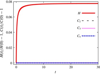
Figure 10 shows the time evolution of the Hamiltonian
 $H$
and several Casimir invariants
 $C_{2}$
,
 $C_{3}$
and
 $C_{4}$
, compared with initial values. We observe that
 $H$
increases monotonically with time
 $t$
while
 $C_{2}$
,
 $C_{3}$
and
 $C_{4}$
remain unchanged. The curves for
 $C_{2}$
,
 $C_{3}$
and
 $C_{4}$
overlap at the zero line of the vertical axis. The stationary state obtained is shown in the
 $x{-}y$
plane in figure 11. The solid curves are contours of
 ${\it\varphi}$
, and the colour map shows the vorticity field
 ${\it\omega}$
.
Time evolution of the Hamiltonian
 $H$
and Casimir invariants
 $C_{2}$
,
 $C_{3}$
and
 $C_{4}$
, compared with initial values. We observe that
 $H$
increases monotonically, while
 $C_{2}$
,
 $C_{3}$
and
 $C_{4}$
are unchanged. Note that the curves for
 $C_{2}$
,
 $C_{3}$
and
 $C_{4}$
overlap at the zero line of the vertical axis.

The stationary state obtained by SA. The solid curves are contours of
 ${\it\varphi}$
, and the colour map shows
 ${\it\omega}$
. This stationary state has
 $C_{1}=0$
,
 $C_{2}=20$
and
 $C_{3}=30$
, which were specified through the adjustment process of the vorticity field. These values, as well as other Casimir invariants, are well conserved during SA.

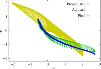
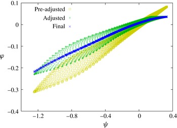
Figure 12 is a scatter plot for
 ${\it\omega}$
and
 ${\it\varphi}$
. As explained in § 2,
 ${\it\varphi}$
becomes a function of
 ${\it\omega}$
at a stationary state. Therefore, the scatter plot between
 ${\it\omega}$
and
 ${\it\varphi}$
should become a curve. As we observe in figure 12,
 ${\it\varphi}$
seems to be a function of
 ${\it\omega}$
at the obtained stationary state indicated by ‘Final’ in the figure. In the same figure, scatter plots of the pre-adjusted and adjusted vorticity fields are shown. As we observe, the pre-adjusted vorticity field is broadly scattered in the plot. Further, even after adjustment,
 ${\it\varphi}$
does not seem to be a function of
 ${\it\omega}$
, because the adjusted vorticity field is clearly not a stationary state.
Scatter plot between
 ${\it\omega}$
and
 ${\it\varphi}$
. At the stationary state obtained, indicated by ‘Final’,
 ${\it\varphi}$
seems to be a function of
 ${\it\omega}$
. Further, the plot of the pre-adjusted and adjusted vorticity fields shows broad scattering, because a stationary state is not attained.

As we observe in figure 12, the relationship between
 ${\it\varphi}$
and
 ${\it\omega}$
at the stationary state is nonlinear. If we try to seek a stationary state with minimal enstrophy, we obtain a linear relationship between
 ${\it\varphi}$
and
 ${\it\omega}$
(Bretherton & Haidvogel Reference Bretherton and Haidvogel1976). In this case we do not care about the Casimir invariants other than enstrophy. On the other hand, our simulation conserves the other Casimir invariants. The conservation of the Casimir invariants may work as a constraint for finding such solutions. A variety of nice stationary states can be obtained by specifying the values of
 $C_{j}$
. Moreover, we obtained this stationary state by maximizing the energy. This fact, together with the relationship between
 ${\it\varphi}$
and
 ${\it\omega}$
, should be related to stability issues via an upper bound on the energy (Shepherd Reference Shepherd1988; Ishioka Reference Ishioka2013). Further, it may be interesting to see our simulation from the perspective of statistical two-dimensional fluid mechanics (Miller Reference Miller1990; Robert & Sommeria Reference Robert and Sommeria1991). These are issues for the future.
5. Numerical results of SA for MHD
In this section we show numerical results for a magnetohydrodynamic (MHD) system in two dimensions. As stated in the Introduction, a two-dimensional MHD equilibrium is normally obtained by solving the G–S equation. Since the G–S equation is elliptic, it is conventionally solved as the Poisson equation. The G–S equation can be extended to include plasma flow. As we will see, however, the extended G–S equation can be hyperbolic when the plasma flow is fast enough. Then we cannot solve to obtain an equilibrium or a stationary state in the conventional way. On the other hand, the SA method is not restricted by the flow speed. Furthermore, as we will explain below, the stationary state presented in this section may be difficult to obtain by solving the extended G–S equation.
The low-beta reduced MHD equations in two dimensions adopted here are
 $$\begin{eqnarray}\displaystyle & \displaystyle \frac{\partial {\it\omega}}{\partial t}=[{\it\omega},{\it\varphi}]+[{\it\psi},J], & \displaystyle\end{eqnarray}$$
 $$\begin{eqnarray}\displaystyle & \displaystyle \frac{\partial {\it\psi}}{\partial t}=[{\it\psi},{\it\varphi}], & \displaystyle\end{eqnarray}$$
 ${\it\omega}:={\rm\Delta}{\it\varphi}$
as in the neutral fluid. In this model, a strong magnetic field is assumed to exist in the
 $z$
direction, perpendicular to the two-dimensional
 $x{-}y$
plane, and thus the magnetic field is given by
 $\boldsymbol{B}=B_{z}\hat{\boldsymbol{z}}+\boldsymbol{{\rm\nabla}}{\it\psi}\times \hat{\boldsymbol{z}}$
. The current density in the
 $z$
direction is given by
 $\hat{\boldsymbol{z}}\boldsymbol{\cdot }\boldsymbol{{\rm\nabla}}\times \boldsymbol{B}=-J$
, where
 $J:={\rm\Delta}{\it\psi}$
.
The low-beta reduced MHD can also be formulated in the Hamiltonian form. By defining the state vector
 $u$
, the Hamiltonian
 $H$
and the anti-symmetric operator
 $\mathscr{J}$
as
 $$\begin{eqnarray}\displaystyle & u:=\left(\begin{array}{@{}c@{}}{\it\omega}\\ {\it\psi}\end{array}\right), & \displaystyle\end{eqnarray}$$
 $$\begin{eqnarray}\displaystyle & \displaystyle H[u]:=-\frac{1}{2}\int _{\mathscr{D}}({\it\omega}({\rm\Delta}^{-1}{\it\omega})+{\it\psi}({\rm\Delta}{\it\psi}))\,\text{d}x\,\text{d}y, & \displaystyle\end{eqnarray}$$
 $$\begin{eqnarray}\displaystyle & \mathscr{J}=\left(\begin{array}{@{}cc@{}}-[{\it\omega},\circ ] & -[{\it\psi},\circ ]\\ -[{\it\psi},\circ ] & 0\end{array}\right), & \displaystyle\end{eqnarray}$$
 $\partial u/\partial t=\mathscr{J}({\it\delta}H/{\it\delta}u)$
. The Casimir invariants are given by
 $$\begin{eqnarray}\displaystyle & \displaystyle C_{1}:=\int _{\mathscr{D}}F({\it\psi})\,\text{d}x\,\text{d}y, & \displaystyle\end{eqnarray}$$
 $$\begin{eqnarray}\displaystyle & \displaystyle C_{2}:=\int _{\mathscr{D}}{\it\omega}G({\it\psi})\,\text{d}x\,\text{d}y, & \displaystyle\end{eqnarray}$$
 $F({\it\psi})$
and
 $G({\it\psi})$
are arbitrary functions of
 ${\it\psi}$
. For example,
 $C_{1}$
becomes the magnetic helicity when
 $F({\it\psi})={\it\psi}$
, and
 $C_{2}$
becomes the cross-helicity when
 $G({\it\psi})={\it\psi}$
. The Hamiltonian description and the Casimir invariants of the reduced MHD systems were found in Morrison & Hazeltine (Reference Morrison and Hazeltine1984).
By defining the energy-Casimir functional as
 $H_{C}:=H+C_{1}+C_{2}$
where the Lagrange multipliers are included in
 $C_{1}$
and
 $C_{2}$
, we obtain equilibrium equations from
 ${\it\delta}H_{C}/{\it\delta}u=0$
:
 $$\begin{eqnarray}\displaystyle & {\it\varphi}=G({\it\psi}), & \displaystyle\end{eqnarray}$$
 $$\begin{eqnarray}\displaystyle & J=F^{\prime }({\it\psi})+{\it\omega}G^{\prime }({\it\psi}). & \displaystyle\end{eqnarray}$$
 $F({\it\psi})$
and
 $G({\it\psi})$
is assumed. If we rewrite
 ${\it\omega}$
in (5.9) as
 ${\it\omega}:={\rm\Delta}{\it\varphi}=G^{\prime }({\it\psi}){\rm\Delta}{\it\psi}+G^{\prime \prime }({\it\psi})|\boldsymbol{{\rm\nabla}}{\it\psi}|^{2}$
, which is obtained from (5.8), we obtain the extended, or flow-modified, reduced G–S equation in the form (Morrison Reference Morrison1986)
 $$\begin{eqnarray}(1-G^{\prime 2}({\it\psi})){\rm\Delta}{\it\psi}=F^{\prime }({\it\psi})+G^{\prime }({\it\psi})G^{\prime \prime }({\it\psi})|\boldsymbol{{\rm\nabla}}{\it\psi}|^{2}.\end{eqnarray}$$
This equation is elliptic when
 $G^{\prime 2}({\it\psi})<1$
, and may be solved as the Poisson equation by assuming the functional forms
 $F({\it\psi})$
and
 $G({\it\psi})$
.
Since the low-beta reduced MHD equations are written in Hamiltonian form, the principle of SA also applies to this system. Although the simplest SA is to replace
 $\mathscr{J}$
by
 $\mathscr{J}^{2}$
in the evolution equation in Hamiltonian form, we adopt an extended version of SA, the symmetric bracket (Flierl & Morrison Reference Flierl and Morrison2012; Chikasue & Furukawa Reference Chikasue and Furukawa2015). Readers can find details of the symmetric bracket in the references cited above. Since this system has a lower bound on the energy (Chikasue & Furukawa Reference Chikasue and Furukawa2015), the energy is decreased in this case.
We show numerical results below. First we adjust the vorticity field to prepare the initial condition for SA. We introduce the functional
 $$\begin{eqnarray}W:=\left(\int _{\mathscr{D}}{\it\omega}\,\text{d}x\,\text{d}y\right)^{2}+\left(\int _{\mathscr{ D}}{\it\omega}{\it\psi}\,\text{d}x\,\text{d}y-c_{CH}\right)^{2}.\end{eqnarray}$$
The first term on the right-hand side is to set the spatial average of
 ${\it\omega}$
to zero. The second term is to set the cross-helicity to a desired value
 $c_{CH}$
. If
 $|c_{CH}|$
is large, the absolute value of
 ${\it\omega}$
becomes large and thus the adjusted initial condition has large kinetic energy. On the other hand, if
 $|c_{CH}|$
is small, the absolute value of
 ${\it\omega}$
becomes small and thus the kinetic energy of the adjusted initial condition tends to be small, although the kinetic energy does not necessarily become zero even when
 $|c_{CH}|=0$
.
Thus we have derived an evolution equation for
 ${\it\omega}$
:
 $$\begin{eqnarray}\frac{\partial {\it\omega}}{\partial {\it\tau}}=-\int _{\mathscr{D}}{\it\omega}\,\text{d}x\,\text{d}y-\left(\int _{\mathscr{D}}{\it\omega}{\it\psi}\,\text{d}x\,\text{d}y-c_{CH}\right){\it\psi}.\end{eqnarray}$$
We have fixed
 ${\it\psi}$
and adjusted
 ${\it\omega}$
only. Thus the magnetic helicity does not change during this adjustment process. Then we can prepare initial conditions with various cross-helicities with fixed magnetic helicity.
(a) Pre-adjusted initial conditions:
 ${\it\varphi}$
is shown by contours and
 ${\it\omega}$
by the colour map. (b) Pre-adjusted initial conditions:
 ${\it\psi}$
is shown by contours and
 $J$
by the colour map. (c) Adjusted to
 $c_{CH}=-1$
:
 ${\it\varphi}$
is shown by contours and
 ${\it\omega}$
by the colour map. (d) Adjusted to
 $c_{CH}=-40$
:
 ${\it\varphi}$
is shown by contours and
 ${\it\omega}$
by the colour map. In this adjustment,
 ${\it\psi}$
was kept unchanged.

Here we show only two examples. One has
 $c_{CH}=-1$
, and the other has
 $c_{CH}=-40$
. The pre-adjusted initial conditions for the two cases are
 $$\begin{eqnarray}{\it\omega}=\left\{\begin{array}{@{}ll@{}}1-\left(\displaystyle \frac{r}{r_{0}}\right)^{2}\quad & (r<r_{0}),\\ 0\quad & (r_{0}\leqslant r),\end{array}\right.\end{eqnarray}$$
and
 ${\it\psi}={\rm\Delta}^{-1}J$
with
 $J(x,y)=4({\it\omega}(y,x)-{\it\omega}_{0})$
. Here,
 ${\it\omega}_{0}$
is the spatial average of
 ${\it\omega}$
,
 $r_{0}:=\sqrt{1+0.6\cos 2{\it\theta}}$
,
 $r=\sqrt{x^{2}+y^{2}}$
and
 ${\it\theta}:=\tan ^{-1}(y/x)$
. The pre-adjusted initial conditions, adjusted initial conditions for
 $c_{CH}=-1$
, and those for
 $c_{CH}=-40$
are shown in figure 13. As indicated above, the adjusted state with
 $c_{CH}=-1$
has much smaller kinetic energy than the magnetic energy. On the other hand, for
 $c_{CH}=-40$
, the kinetic energy of the adjusted state is much larger than the magnetic energy. As we will see below, we obtain a non-trivial stationary state by adjusting the initial condition with large
 $|c_{CH}|$
.
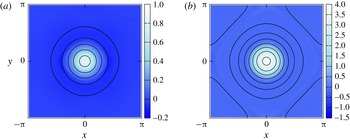
Now we present the stationary state obtained after SA. Figure 14 shows the stationary state with
 $c_{CH}=-1$
. We observe that the final state has a concentric structure. We also show the scatter plot between
 ${\it\varphi}$
and
 ${\it\psi}$
in figure 15. At the final state, we observe that
 ${\it\varphi}$
seems to be a single-valued function of
 ${\it\psi}$
.
Stationary state obtained with
 $c_{CH}=-1$
: (a)
 ${\it\varphi}$
is shown by contours and
 ${\it\omega}$
by the colour map; (b)
 ${\it\psi}$
is shown by contours and
 $J$
by the colour map.

Scatter plot between
 ${\it\varphi}$
and
 ${\it\psi}$
for
 $c_{CH}=-1$
. At the final state, we observe that
 ${\it\varphi}$
seems to be a single-valued function of
 ${\it\psi}$
.

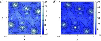
Similarly, figure 16 shows the stationary state for
 $c_{CH}=-40$
. In this case, the stationary state has a smaller-scale structure, unlike the
 $c_{CH}=-1$
case. The structure of the stationary state is determined by the balance between the decrease of kinetic energy and magnetic energy, together with the restriction between velocity and magnetic fields at the stationary state. Since the kinetic energy is given by
 $(\sum _{k}(|{\it\omega}_{k}|^{2}/k^{2}))/2$
by the Fourier representation, small
 $k$
components should become small to decrease the kinetic energy. On the other hand, the magnetic energy is given by
 $(\sum _{k}k^{2}|{\it\psi}_{k}|^{2})/2$
by the Fourier representation. Thus large
 $k$
components should become small to decrease the magnetic energy. However, velocity and magnetic fields must satisfy a relation
 ${\it\varphi}=G({\it\psi})$
at a stationary state. Therefore
 ${\it\omega}$
and
 ${\it\psi}$
cannot evolve independently, and the final structure is determined by their balance. Details of the relaxation process are found in Chikasue & Furukawa (Reference Chikasue and Furukawa2015).
Stationary state obtained with
 $c_{CH}=-40$
: (a)
 ${\it\varphi}$
is shown by contours and
 ${\it\omega}$
by the colour map; (b)
 ${\it\psi}$
is shown by contours and
 $J$
by the colour map.

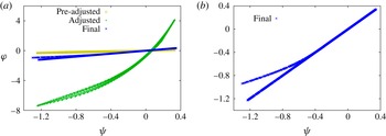
Figure 17 shows the scatter plot between
 ${\it\varphi}$
and
 ${\it\psi}$
. In figure 17(b) only the final state is plotted. We observe that
 ${\it\varphi}$
is clearly a double-valued function of
 ${\it\psi}$
. Since we rely on the differentiability of
 ${\it\varphi}=G({\it\psi})$
in deriving the flow-modified reduced G–S equation, this kind of multi-valued functional form cannot be assumed. Of course, if we divide the domain into several areas, and if we assume
 ${\it\varphi}=G_{1}({\it\psi})$
in some areas and
 ${\it\varphi}=G_{2}({\it\psi})$
elsewhere, where
 $G_{1}({\it\psi})$
and
 $G_{2}({\it\psi})$
are single-valued functions, we may obtain this kind of stationary state by solving the flow-modified reduced G–S equation. However, it may not be so simple to obtain it in reality because (i) we do not know a priori how to divide the domain, and (ii) we can impose only
 ${\it\psi}$
and/or its spatial derivative as the boundary condition in solving the flow-modified reduced G–S equation, so we cannot impose continuity of
 ${\it\omega}$
and
 $J$
across the boundaries of the areas. Therefore, the obtained stationary state is non-trivial. We obtained this stationary state by adjusting the initial condition for the SA to have large cross-helicity.
Scatter plot between
 ${\it\varphi}$
and
 ${\it\psi}$
for
 $c_{CH}=-40$
. In (b), only the final state is plotted. We observe that
 ${\it\varphi}$
is clearly double-valued function of
 ${\it\psi}$
.

6. Conclusions
We have developed a method to adjust a vorticity field that satisfies desired values for a finite number of Casimir invariants. The steepest descent method was utilized. We have demonstrated that the method actually succeeded in specifying values of several Casimir invariants of the vorticity field. The vorticity field was adopted as an initial condition for SA. Thus we obtained a stationary state of an incompressible, ideal neutral fluid in two dimensions that has specified values for some Casimir invariants. We also applied the developed method and SA to low-beta reduced MHD in two dimensions. By specifying the cross-helicity, which is a Casimir invariant, we obtained a non-trivial stationary state which might be difficult to obtain by conventional methods.
Acknowledgements
This work was supported by JSPS KAKENHI grant no. 23760805. The authors thank Professor P. J. Morrison and members of the Plasma Physics Laboratory, Graduate School of Frontier Sciences, University of Tokyo for fruitful discussions. The authors are also grateful for the comments of the referees.