1. Introduction
The evolution of surface waves can be represented by an equation for the action spectral density,
 $N(k,{\it\theta})$
,
 $$\begin{eqnarray}\frac{\partial N(k,{\it\theta})}{\partial t}+(\boldsymbol{c}_{g}+\boldsymbol{U})\boldsymbol{\cdot }\boldsymbol{{\rm\nabla}}N(k,{\it\theta})=-\boldsymbol{{\rm\nabla}}_{k}T(k,{\it\theta})+S_{w}-D,\end{eqnarray}$$
with
 $$\begin{eqnarray}N=(g/k)^{1/2}F,\end{eqnarray}$$
where
 $F(k,{\it\theta})$
is the energy density,
 $T(k,{\it\theta})$
is the spectral flux of action through the wavenumber
 $\boldsymbol{k}=(k,{\it\theta})$
by nonlinear wave–wave interactions,
 $\boldsymbol{c}_{g}$
is the group velocity,
 $\boldsymbol{U}$
is the current,
 $S_{w}$
is the input from the wind and
 $D$
is the dissipation due to breaking or the formation of parasitic capillaries as recognized by Phillips (Reference Phillips1985). Phillips’ paper considered equilibrium models of the wind-wave spectrum in which the left-hand side of (1.1) is zero. It also introduced a statistical description of breaking based on
 ${\it\Lambda}(\boldsymbol{c})\text{d}\boldsymbol{c}$
, the average length of breaking fronts per unit area of ocean surface moving with velocity in the range
 $(\boldsymbol{c},\boldsymbol{c}+\text{d}\boldsymbol{c})$
. This introduction of
 ${\it\Lambda}(\boldsymbol{c})$
has prompted many attempts to measure it (i.e. breaking kinematics) in the field and also the use of laboratory measurements to quantify a dimensionless breaking strength parameter,
 $b$
, defined by
 $$\begin{eqnarray}{\it\epsilon}_{l}=b{\it\rho}_{w}g^{-1}c^{5},\end{eqnarray}$$
where
 ${\it\epsilon}_{l}$
is the rate of wave energy dissipation per unit length of breaking crest,
 ${\it\rho}_{w}$
is the mass density of water and
 $c\equiv |\boldsymbol{c}|$
is the phase speed.
Based on inertial arguments and the measurements of Melville (Reference Melville1994) and Drazen, Melville & Lenain (Reference Drazen, Melville and Lenain2008), which showed that for moderately strong to very strong breaking waves the breaking strength
 $b\propto S^{5/2}$
, and with the measurements of Banner & Peirson (Reference Banner and Peirson2007), Romero, Melville & Kleiss (Reference Romero, Melville and Kleiss2012) have shown that, within the scatter of the data,
 $$\begin{eqnarray}b=A(S-S_{0})^{5/2}\end{eqnarray}$$
applies over all the available laboratory data, where
 $S$
, an external control parameter, is a characteristic linear slope of a focusing wave group at breaking,
 $A=0.4$
and
 $S_{0}=0.08$
is a threshold slope. The more recent laboratory data of Grare et al. (Reference Grare, Peirson, Branger, Walker, Giovangeli and Makin2013) support (1.4), as does the numerical modelling of Deike, Popinet & Melville (Reference Deike, Popinet and Melville2015).
Using field measurements of
 $N(k,{\it\theta})$
and
 ${\it\Lambda}(\boldsymbol{c})$
from whitecap kinematics, computation of the wave–wave interactions and standard models of
 $S_{w}$
, Romero et al. (Reference Romero, Melville and Kleiss2012) used a steady version of (1.1) to estimate
 $D$
. However, it was found that the dynamics could not be closed at shorter wavelengths, say around 50 cm and less, with the whitecap-based measurements of
 ${\it\Lambda}(\boldsymbol{c})$
. Very recently, using stereo infrared imaging of the ocean surface, Sutherland & Melville (Reference Sutherland and Melville2013) have shown that non-air-entraining breaking significantly increases
 ${\it\Lambda}(\boldsymbol{c})\text{d}\boldsymbol{c}$
at small values of
 $c$
, consistent with the modelling of Romero et al. (Reference Romero, Melville and Kleiss2012), but does not yet reach into the shorter gravity–capillary wavelengths of
 $O(10)$
cm and less considered here.
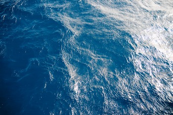
Photograph of the sea surface taken from the bow of the R/V Revelle on the equator at 140°W in winds of approximately
 $7~\text{m}~\text{s}^{-1}$
, on 18 October 2012, at approximately 1530 local time. The sun is shining from the right-hand side of the scene. Note the fine-scale structure of the wave field at the surface, especially surface waves of length
 $O(10)$
cm. (Photo: Nicholas Statom, Scripps Institution of Oceanography.)

One interpretation of these results is that wave dissipation due to microscale breaking with no significant air entrainment (Banner & Phillips Reference Banner and Phillips1974) may be dominant at these scales. Such breaking may result from the instability of parasitic capillary waves generated on the forward faces of short gravity–capillary waves (Longuet-Higgins Reference Longuet-Higgins1992; Duncan et al.
Reference Duncan, Philomin, Behres and Kimmel1994, Reference Duncan, Qiao, Philomin and Wenz1999; Fedorov, Melville & Rozenberg Reference Fedorov, Melville and Rozenberg1998 (hereafter FMR98); Perlin et al.
Reference Perlin, Jiang, Lin and Schultz1999; Perlin & Schultz Reference Perlin and Schultz2000; Tsai & Hung Reference Tsai and Hung2010). Even in the absence of breaking, it has been shown that parasitic capillaries may lead to significantly enhanced damping of longer gravity–capillary waves (Ruvinsky, Feldstein & Freidman Reference Ruvinsky, Feldstein and Freidman1991; Longuet-Higgins Reference Longuet-Higgins1995; Fedorov & Melville Reference Fedorov and Melville1998 (hereafter FM98)). Figure 1 shows an image of the ocean surface and gravity–capillary waves of these
 $O(1{-}10)$
cm scales riding on longer waves.
In a study of steady gravity–capillary waves with pressure forcing at the surface and viscous dissipation in the surface boundary layer, Fedorov & Melville (Reference Fedorov and Melville1998) found that under sufficiently strong forcing, and hence dissipation, strongly asymmetric solutions for the wave profile can be found with steep forward faces modulated by parasitic capillary waves and long upwind surfaces of smaller slope. The dissipation in these solutions is predominantly in the neighbourhood of the parasitic capillaries. In effect, the regions of high surface curvature and vorticity associated with the capillary waves may provide the dissipation that at longer wavelengths may be afforded by air-entraining breaking.
Since FM98 and FMR98 there have been laboratory experiments on the dissipation due to parasitic capillaries by Zhang (Reference Zhang2002), who measured the energy dissipation rate normalized by the linear value and fitted his data with a polynomial to second order in the wave slope,
 $ak-S_{0}$
, where
 $S_{0}=0.05$
is a small offset. Zhang used Longuet-Higgins’ (Reference Longuet-Higgins1995) theory and the measurements of FMR98 to estimate the dissipation, but from those data and his own measurements he concluded that ‘for a conclusive estimation of capillary dissipation, a larger number of measured surface slope profiles are needed’. However, he also noted that the parasitic capillary wave slopes are dependent on the long (gravity) wave parameters. Tsai & Hung (Reference Tsai and Hung2010) conducted direct numerical simulations (DNS) of gravity–capillary waves and computed normalized energy dissipation rates, which they too fitted with a polynomial, but this time using the mean slope of all the capillary waves as the independent variable. However, the detailed measurements of the parasitic capillaries are notoriously difficult, and they did not collapse their results onto the parameters of the underlying gravity waves. Since neither Zhang (Reference Zhang2002) nor Tsai & Hung (Reference Tsai and Hung2010) directly compared their results with those of FM98, it is difficult to compare their results with this work, which is based on FM98. Nor did they attempt to place their results in the context of the wind-wave problem.
As far as we are aware, then, no direct predictions have been made to confirm that the dissipative effects of the parasitic capillaries are sufficient to balance the observed and predicted growth of the short
 $O(1{-}10)$
cm gravity–capillary waves, given the uncertainties in both. That is the primary aim of this paper. This is one aspect of the ‘saturation’ problem in the theory of wind-wave modelling. In other words, is there a rational dissipative process to balance the wind input at these short gravity–capillary wave scales? We believe that this question can be addressed without the need to construct a full wind-wave model that includes all the nonlinear processes that can transfer wave energy to other scales via slow weakly nonlinear three- and four-wave resonances (see e.g. Janssen Reference Janssen2004). Parasitic capillaries are generated on a fast time scale as the result of a direct resonance between the gravity and capillary waves. This paper does not attempt to construct a new semi-empirical wind-wave model, but rather seeks to determine whether the dissipation due to parasitic capillaries is significant in the energy balance of the short,
 $O(10)$
cm, gravity–capillary waves, by using comparisons with the measured and modelled wind input and with dissipation due to breaking.
These shorter gravity wave lengths also arise in measurements of the slope statistics of the sea surface. The classical paper is that of Cox & Munk (Reference Cox and Munk1954, hereafter CM54), who conducted airborne measurements of sun glitter. The location of the glitter relative to the specular reflection of the sun from a horizontal plane surface is a measure of the slope of the surface at that point. Hence the slope statistics can be calculated from images of the sun glitter. CM54 showed that, in wind speeds up to
 $14~\text{m}~\text{s}^{-1}$
(measured 12 m above the surface), the mean square slope (MSS) of the sea surface is proportional to
 $U$
, the wind speed at 12 m, and that when covered with an oil slick the waves shorter than approximately 30 cm are suppressed and the MSS is reduced by approximately 60 % at a wind speed of
 $10~\text{m}~\text{s}^{-1}$
. The MSS results of CM54 in the absence of anthropogenic oil slicks have been confirmed by recent satellite observations comprising a much larger data set (Bréon & Henriot Reference Bréon and Henriot2006). In fact, the MSS results of CM54 are used to tune many wind-wave models and remote-sensing algorithms of ocean winds and surface processes.
In this paper we use the theory of FM98 to predict the dissipation due to viscosity in steady surface-pressure-forced equilibrium solutions of gravity–capillary waves that include parasitic capillaries at stronger forcing and larger underlying wave slopes. In § 2 the FM98 theory and its numerical solutions are briefly reviewed. In § 3 we compare the predicted dissipation as a function of wave age and wave slope with the wind input data collated by Plant (Reference Plant1982), and the modelling of Miles (Reference Miles1959, Reference Miles1993) and Yang, Meneveau & Shen (Reference Yang, Meneveau and Shen2013). We also consider the dependence of the MSS of the short gravity–capillary waves on
 $u_{\ast }$
. In § 4 we review and discuss the results, including the MSS in the predictions of the FM98 model and the measurements of MSS in CM54.
2. The theoretical model and basic results
2.1. The Fedorov & Melville (Reference Fedorov and Melville1998) theoretical model
The FM98 theory addresses nonlinear steady periodic gravity–capillary waves of permanent form in a frame of reference travelling with the phase speed
 $c$
to the right
 $(c>0)$
. The approach is classical, with an outer irrotational flow except in a thin viscous boundary layer at the surface of the fluid. It is also assumed that, to the leading order, all Fourier components of the wave are damped independently, a linear damping assumption that neglects higher-order nonlinear dissipative terms. This is the only linear assumption in the theory – otherwise it is fully nonlinear. An independent source of energy is required to balance the dissipation and give a steady solution. This is done with an external sinusoidal pressure force at the surface of the same wavelength as the basic wave, so higher harmonics of the wave, including any parasitic ripples, are not directly affected by the forcing.
With these assumptions and approximations, a closed set of equations yields a parametric description of the two-dimensional surface
 $$\begin{eqnarray}X=X({\it\zeta}),\quad Y=Y({\it\zeta}),\end{eqnarray}$$
or
 $$\begin{eqnarray}Z=X+\text{i}Y,\end{eqnarray}$$
where
 $X$
and
 $Y$
are the horizontal and vertical coordinates of the surface, and
 ${\it\zeta}$
is the independent parameter. The full details of the derivation of the theoretical model are given in FM98 and yield this final formulation.
One must find
 $Z^{i}$
, such that
 $$\begin{eqnarray}Z^{i}=\frac{1}{k}\left({\it\zeta}+\text{i}\mathop{\sum }_{m=1}^{\infty }a_{m}\text{e}^{-\text{i}m{\it\zeta}}\right),\quad {\it\zeta}\subset [0,2{\rm\pi}]\end{eqnarray}$$
and
 $$\begin{eqnarray}\frac{U^{i2}}{2}+gY+\frac{{\it\Gamma}}{R}+\frac{P_{0}}{{\it\rho}_{w}}+\frac{{\it\nu}k}{c}\frac{\partial }{\partial {\it\zeta}}U^{i2}=E,\end{eqnarray}$$
where
 $$\begin{eqnarray}\displaystyle & \displaystyle U^{i}=-\frac{c}{k}(Z_{{\it\zeta}}^{i}Z_{{\it\zeta}}^{i\ast })^{-1/2}, & \displaystyle\end{eqnarray}$$
 $$\begin{eqnarray}\displaystyle & \displaystyle Z=Z^{i}-\frac{2\text{i}{\it\nu}}{c^{2}k}\int _{0}^{{\it\zeta}}\left(\frac{U^{i}}{R^{i}}-\left\langle \frac{U^{i}}{R^{i}}\right\rangle \right)\!\text{d}{\it\zeta}^{\prime }, & \displaystyle\end{eqnarray}$$
 $$\begin{eqnarray}\displaystyle & \displaystyle \frac{1}{R}=-\text{Im}\{Z_{{\it\zeta}{\it\zeta}}Z_{{\it\zeta}}^{-3/2}Z_{{\it\zeta}}^{\ast -1/2}\}, & \displaystyle\end{eqnarray}$$
 $$\begin{eqnarray}\displaystyle & \displaystyle P_{0}=\tilde{P}_{0}\cos kX, & \displaystyle\end{eqnarray}$$
 $$\begin{eqnarray}\displaystyle X=\text{Re}\,Z-\text{Re}\,Z|_{{\it\zeta}=0}\quad \text{and}\quad Y=\text{Im}\,Z, & & \displaystyle\end{eqnarray}$$
 $$\begin{eqnarray}\displaystyle \frac{1}{R^{i}}=-\text{Im}\{Z_{{\it\zeta}{\it\zeta}}^{i}Z_{{\it\zeta}}^{i-3/2}Z_{{\it\zeta}}^{i\ast -1/2}\} & & \displaystyle\end{eqnarray}$$
and
 $$\begin{eqnarray}\left\langle \frac{U^{i}}{R^{i}}\right\rangle =\frac{1}{2{\rm\pi}}\int _{0}^{2{\rm\pi}}\frac{U^{i}}{R^{i}}\,\text{d}{\it\zeta}^{\prime }.\end{eqnarray}$$
Here
 ${\it\Gamma}$
is the surface tension;
 $P_{0}$
is the external pressure forcing at the surface required to balance the wave dissipation;
 $U^{i}$
,
 $Z^{i}$
and
 $R^{i}$
are the irrotational component of the flow velocity on the surface, the complex coordinate of the surface and the local radius of curvature, respectively; and
 $R$
is the full radius of curvature of the surface. Equation (2.3) is the Stokes expansion with the
 $a_{m}$
to be determined; (2.4) is Bernoulli’s equation with the unknown constant
 $E$
. When
 $a_{m}$
,
 $c$
and
 $E$
are solved for,
 $Z^{i}$
is determined from (2.3),
 $Z$
is calculated and the surface profile is given by (2.1).
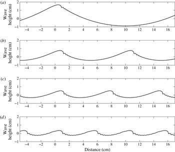
Profiles of steady gravity–capillary wave solutions obtained from the model for: (a)
 ${\it\lambda}=20~\text{cm}$
,
 $ak=0.40$
; (b)
 ${\it\lambda}=10~\text{cm}$
,
 $ak=0.375$
; (c)
 ${\it\lambda}=7~\text{cm}$
,
 $ak=0.375$
; and (d)
 ${\it\lambda}=5~\text{cm}$
,
 $ak=0.375$
.

The non-dimensional wave amplitude (or ‘characteristic slope’) of the wave of length
 ${\it\lambda}=2{\rm\pi}/k$
is given by
 $$\begin{eqnarray}ak=[\max Y-\min Y]k/2,\end{eqnarray}$$
and the non-dimensional amplitude of the pressure forcing is defined by
 $$\begin{eqnarray}p=\frac{\tilde{P}_{0}}{{\it\rho}_{w}c_{0}^{2}},\end{eqnarray}$$
where
 $$\begin{eqnarray}c_{0}=\sqrt{\frac{g}{k}+{\it\Gamma}k}=\sqrt{\frac{g}{k}}\,\sqrt{1+\mathit{ Bo }^{-1}}=\sqrt{\frac{g^{\prime }}{k}},\end{eqnarray}$$
is the phase speed of linear gravity–capillary waves,
 $\mathit{Bo}=g/({\it\Gamma}k^{2})$
is the Bond number and
 $g^{\prime }=g(1+\mathit{Bo}^{-1})$
is a modified gravity.
With
 ${\it\rho}_{w}=1000~\text{kg}~\text{m}^{-3}$
,
 ${\it\Gamma}=73\times 10^{-6}~\text{m}^{3}~\text{s}^{-2}$
and
 ${\it\nu}=10^{-6}~\text{m}^{2}~\text{s}^{-1}$
all fixed, the solutions have a parametric dependence on
 ${\it\lambda}$
,
 $p$
and
 $ak$
. The system is discretized with
 $O(100{-}1000)$
points on the interval of
 ${\it\zeta}$
from
 $0$
to
 $2{\rm\pi}$
and solved using Newton’s method. Examples of solutions for
 ${\it\lambda}=5$
, 7, 10 and 20 cm with
 $ak=0.375$
or 0.4 are shown in figure 2. Note the high curvature in the troughs of the parasitic capillaries, which is associated with the regions of high vorticity and dissipation. At stronger forcing, a separate class of solutions was obtained with members not topologically connected to these solutions, and consisted of small capillary ‘bumps’ separating longer waves. Details are given in FM98.
2.2. Wave energy, surface pressure work and wave dissipation
The energy density of the surface wave is
 $$\begin{eqnarray}E_{W}=E_{K}+E_{G}+E_{T},\end{eqnarray}$$
where
 $E_{K}$
,
 $E_{G}$
and
 $E_{T}$
are the mean densities of kinetic energy, potential energy due to gravity and potential energy due to surface tension, respectively. Formulas for these variables are given correct to leading order in
 ${\it\gamma}=k{\it\delta}$
in FM98, where
 ${\it\delta}$
is the characteristic thickness of the viscous boundary layer in the water,
 $E_{K}$
is calculated in the fixed frame, and the average surface elevation
 $\overline{Y}={\it\lambda}^{-1}\int _{0}^{{\it\lambda}}Y\text{d}X=0$
.
The rate of working
 ${\dot{E}}_{W}$
per unit area due to the surface pressure is given by
 $$\begin{eqnarray}{\dot{E}}_{W}=\frac{c}{{\it\lambda}}\int _{0}^{{\it\lambda}}P_{0}\,\text{d}Y=\frac{c}{{\it\lambda}}\int _{0}^{{\it\lambda}}\tilde{P}_{0}\cos (kX)\text{d}Y,\end{eqnarray}$$
which is balanced by the viscous dissipation of energy in the boundary layer and includes the effects of the parasitic capillaries when they are generated. Given this balance, these energy fluxes can be represented by a dimensionless growth or dissipation rate of energy per wave period of
 $$\begin{eqnarray}{\it\beta}=\frac{2{\rm\pi}}{{\it\sigma}}\frac{{\dot{E}}_{W}}{E_{W}},\end{eqnarray}$$
where
 ${\it\sigma}=kc$
is the radian frequency.
The momentum flux due to the pressure forcing can also be expressed as a wave-coherent surface stress defining a friction velocity
 $u_{\ast w}$
:
 $$\begin{eqnarray}{\it\tau}_{w}\equiv {\it\rho}_{a}u_{\ast w}^{2}=\frac{1}{{\it\lambda}}\int _{0}^{{\it\lambda}}\left(P_{0}\frac{\text{d}Y}{\text{d}X}\right)\!\text{d}X=\left\langle P_{0}\frac{\text{d}Y}{\text{d}X}\right\rangle ,\end{eqnarray}$$
where
 ${\it\rho}_{a}$
is the density of the air and
 $\langle \cdots \rangle$
denotes the spatial average. Consequently,
 $$\begin{eqnarray}{\dot{E}}_{W}=c{\it\tau}_{w}=c{\it\rho}_{a}u_{\ast w}^{2}.\end{eqnarray}$$
For linear gravity–capillary waves with no parasitic capillaries (Phillips Reference Phillips1977),
 $$\begin{eqnarray}{\dot{E}}_{W}=2{\it\nu}k^{3}a^{2}{\it\rho}_{w}c_{0}^{2},\end{eqnarray}$$
and equating (2.19) and (2.20) gives
 $$\begin{eqnarray}u_{\ast w}=ak\sqrt{2\frac{{\it\rho}_{w}}{{\it\rho}_{a}}c_{0}{\it\nu}k}.\end{eqnarray}$$
For weakly nonlinear gravity–capillary waves (Hogan Reference Hogan1980)
 $$\begin{eqnarray}E_{W}={\textstyle \frac{1}{2}}{\it\rho}_{w}a^{2}g^{\prime }(1+O(ak)^{2})={\textstyle \frac{1}{2}}{\it\rho}_{w}a^{2}kc^{2}(1+O(ak)^{2}).\end{eqnarray}$$
From (2.20) and (2.22) for linear gravity–capillary waves,
 $$\begin{eqnarray}\frac{{\dot{E}}_{W}}{E_{W}}=4{\it\nu}k^{2}\quad \text{and}\quad {\it\beta}=\frac{8{\rm\pi}k{\it\nu}}{c_{0}}.\end{eqnarray}$$
More generally, from (2.19) and (2.22),
 $$\begin{eqnarray}\displaystyle {\it\beta} & = & \displaystyle 4{\rm\pi}\frac{{\it\rho}_{a}}{{\it\rho}_{w}}\left(\frac{u_{\ast w}}{c}\right)^{2}\left(\frac{1}{ak}\right)^{2}(1+O(ak)^{2})\end{eqnarray}$$
 $$\begin{eqnarray}\displaystyle & = & \displaystyle 4{\rm\pi}{\it\chi}\frac{{\it\rho}_{a}}{{\it\rho}_{w}}\left(\frac{u_{\ast }}{c}\right)^{2}\left(\frac{1}{ak}\right)^{2}(1+O(ak)^{2}),\end{eqnarray}$$
 $$\begin{eqnarray}{\it\chi}\equiv \left(\frac{u_{\ast w}}{u_{\ast }}\right)^{2}\end{eqnarray}$$
is the ratio of the wave-coherent momentum flux to the total momentum flux across the surface. For the numerical results presented here,
 ${\it\chi}=1$
, since the wave-coherent pressure forcing, which is a part of the solution, is the only momentum flux across the surface.
Finally, for
 $Y=a\cos kX$
, the mean square slope for linear waves (limited here to the
 $x$
component) is given by
 $$\begin{eqnarray}s_{x}^{2}\equiv \frac{1}{{\it\lambda}}\int _{0}^{{\it\lambda}}\left(\frac{\text{d}Y}{\text{d}X}\right)^{2}\!\text{d}X=\frac{(ak)^{2}}{2}=\frac{{\it\rho}_{a}}{4{\it\rho}_{w}}\frac{u_{\ast w}^{2}}{c_{0}{\it\nu}k}.\end{eqnarray}$$
2.3. Momentum flux
In (2.18) we introduced the wave-coherent momentum flux, which in this problem is the total momentum flux across the surface. However, in the laboratory or field environment, the total momentum flux comprises viscous, wave and turbulent fluxes, to give a total flux of
 ${\it\tau}\equiv {\it\rho}_{a}u_{\ast }^{2}$
, which defines the (total) friction velocity
 $u_{\ast }$
. To maintain a clear separation between
 $u_{\ast }$
and
 $u_{\ast w}$
, we defined the ratio of wave-coherent momentum flux to total momentum flux,
 ${\it\chi}$
, with
 ${\it\chi}\leqslant 1$
in general, while
 ${\it\chi}=1$
in FM98.
Equation (2.25) for
 ${\it\beta}$
shows that if the wave age
 $c/u_{\ast }$
and slope
 $ak$
are given then the crux of the wave growth problem resides in predicting
 ${\it\chi}$
. Furthermore, if
 ${\it\beta}$
is to remain finite, then
 ${\it\chi}\propto (ak)^{2}$
as
 $ak\downarrow 0$
in the linear limit. In FM98,
 $u_{\ast }=u_{\ast w}$
is not given but is a part of the solution to balance the viscous dissipation.
There is another aspect of the momentum flux that needs discussion and that is the conservation of momentum in FM98. The theory neglects the continuing diffusion of momentum and vorticity into the interior of the fluid over long times, which is an
 $O({\it\epsilon}^{2})$
effect, where
 ${\it\epsilon}$
is a measure of the wave slope. Thus the theory applies only for relatively short times. Over much longer times, sufficient for diffusive effects to reach the full depth, the momentum flux can be balanced by the static pressure differences in the water associated with the mean slope of the surface over many wavelengths. This slope tends to zero as the water depth tends to infinity (Donelan et al.
Reference Donelan, Haus, Reul, Plant, Stiassnie, Graber, Brown and Saltzman2004).
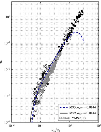
Dimensionless growth rate of wave energy versus the reciprocal wave age,
 $u_{\ast }/c_{0}$
. Collation of field data (open black symbols) and laboratory data (solid black symbols and crosses) by Plant (Reference Plant1982) plotted with Miles’ (Reference Miles1959; Reference Miles1993) theory for a Charnock constant
 ${\it\alpha}_{CH}=0.0144.$
See Komen et al. (Reference Komen, Cavaleri, Donelan, Hasselmann, Hasselmann and Janssen1994) and Janssen (Reference Janssen2004). Also shown as grey symbols (YMS2013) are the numerical solutions of Yang et al. (Reference Yang, Meneveau and Shen2013).

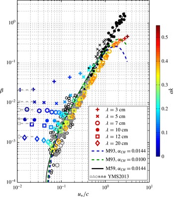
Dimensionless growth rate of wave energy versus the reciprocal wave age,
 $u_{\ast }/c_{0}$
, of figure 3, but now including the predictions of the FM98 theory in colour according to the slope scale to the right, and Miles’ (Reference Miles1993) model that extends Miles’ (Reference Miles1959) model by including the effects of modulation of turbulent Reynolds stresses by the waves. Note that
 $c$
rather than
 $c_{0}$
is used for the FM98 results; see text. The values on the vertical axis, marked in grey rather than colour, correspond to the growth rates for linear gravity waves without the effects of parasitic capillaries. The grey symbols (YMS2013) in the main body of the plot are the numerical predictions of Yang et al. (Reference Yang, Meneveau and Shen2013) as in figure 3. Note that for
 $0.07<u_{\ast }/c<1$
and
 $0.2<ak<0.4$
the
 ${\it\beta}$
predicted by FM98 is largely within the scatter of the measurements and a factor of approximately 2 of Miles’ (Reference Miles1993) results over this range of wave ages
 $(0.5<{\it\beta}_{M93}/{\it\beta}_{FM98}<2)$
, whereas the results of Yang et al. (Reference Yang, Meneveau and Shen2013) show
 $0.7<{\it\beta}_{M93}<5.5$
over the same range of
 $u_{\ast }/c$
; see Discussion in § 4.

3. Results
3.1. Balancing wave growth data with dissipation due to parasitic capillaries
The primary aim of this work is to determine whether the dissipation due to parasitic capillary waves predicted by the FM98 model is sufficient to balance the wind input to the shorter gravity wave lengths.
Plant’s (Reference Plant1982) collation of both laboratory and field measurements of the dimensionless rate of wave growth as a function of reciprocal wave age
 ${\it\beta}={\it\beta}(u_{\ast }/c_{0})$
remains the primary collection of laboratory and field data and has been used to compare with the available theory. However, recently, Yang et al. (Reference Yang, Meneveau and Shen2013) have also predicted
 ${\it\beta}$
using coupled numerical solutions to the wind-driven boundary layer in the air and irrotational waves in the water, and their results are also shown in figures 3 and 4. Figure 3 shows a version of Plant’s collation drawn from Janssen (Reference Janssen2004) and includes the prediction of Miles’ (Reference Miles1959) quasi-laminar model including viscous stresses for a given Charnock parameter,
 ${\it\alpha}_{CH}\equiv gz_{0}/u_{\ast }^{2}=0.0144$
, where
 $z_{0}$
is the roughness length in the atmospheric logarithmic boundary layer above the waves. Miles’ (Reference Miles1993) model results, also shown with the same Charnock parameter, include the modulation of turbulent Reynolds stresses by the waves. The scatter in the laboratory data is relatively small, while that in the field data is up to an order of magnitude, but these are very difficult measurements to make, and Miles’ theories, which do not account for wave slope effects, appear, within the limits of the scatter, to span both sets of data.
In figure 4, the results of the FM98 equilibrium theory for the wave growth (2.25), which is balanced by the viscous dissipation, is plotted as a function of the wavelength and the reciprocal wave age and slope and overlaid on figure 3 along with the results of Miles’ (Reference Miles1959, Reference Miles1993) theories, the latter for two values of
 ${\it\alpha}_{CH}$
. See also the numerical results of Yang et al. (Reference Yang, Meneveau and Shen2013). Miles’ 1993 theory differs from that of 1959 by the addition of the modulation of the turbulent Reynolds stresses by the wave field, an effect that Miles expected to apply to the longer waves. The FM98 results, which include the computed nonlinear phase speed
 $c$
, show that as the wave slope tends to zero the dimensionless growth/dissipation rate approaches the linear result given by (2.23). As the forcing and slope increase, for the shortest 3 cm waves the effects of capillary waves quickly become significant, with the dissipation rate increasing quickly. For the 5 cm waves, there is initially little change in the dissipation rate at smaller slopes, again increasing when the effects of the parasitic capillaries become apparent. Moving to longer gravity waves, there is an initial decrease in the dissipation rate, reaching a minimum before yet again the increased dissipation due to the capillary waves takes effect. In general, at the larger slopes the effects of parasitic capillaries become active, the growth (decay) rate increases and within the approximate range of slopes,
 $0.2<ak<0.4$
, the FM98 results are largely within the range of the measurements. Over that range of slopes and for
 $0.07<u_{\ast }/c<2$
, our model results are on average less than those of Miles (Reference Miles1993) by a factor of 0.78, and larger than the Yang et al. (Reference Yang, Meneveau and Shen2013) results over the available range
 $0.07<u_{\ast }/c<0.5$
by a factor of 1.25. At larger slopes, our results diverge from the laboratory measurements and Miles’ (Reference Miles1959) predictions but intersect Miles’ (Reference Miles1993) model results.
The implication of the comparison of FM98 with the data is that, for wavelengths in the range
 $3<{\it\lambda}<20~\text{cm}$
and slopes in the range
 $0.2<ak<0.4$
, the dissipation due to the parasitic capillary waves in the FM98 equilibrium model would, to within a factor of order unity, be sufficient to balance the wind input measurements at these wavelengths, in agreement with recent numerical model results of wave growth and dissipation reported in the literature (Yang et al.
Reference Yang, Meneveau and Shen2013; Deike et al.
Reference Deike, Popinet and Melville2015). This is the primary result of this paper.
3.2. Scaling of wave growth and dissipation with wave age and wave slope
Plant’s (Reference Plant1982) figure was constructed in the context of comparison with linear theory, and therefore any dependence of the data on wave slope is embedded in the scatter of the data. However, with (2.25), we have a dependence of
 ${\it\beta}$
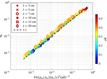
on both wave age and wave slope for weakly nonlinear gravity waves. In figure 5, we plot
 ${\it\beta}$
versus
 $4{\rm\pi}({\it\rho}_{a}/{\it\rho}_{w})(u_{\ast }/c)^{2}(ak)^{-2}$
for the nonlinear FM98 predictions, where
 $c$
is the phase speed computed from the theory, not the linear phase speed,
 $c_{0}$
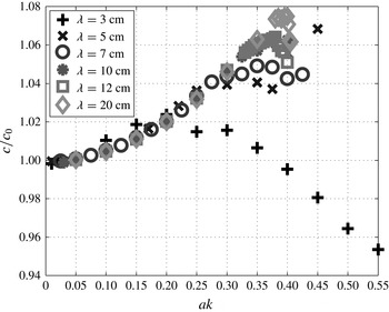
. From the log–log plot of figure 5, we see that this relationship gives leading-order scaling across the whole range of wavelengths, wave ages and wave slopes. However, a linear plot (figure 6) shows that the normalized differences are of
 $O(ak)$
over the range of slopes considered. Again, in figure 6, as in figure 4, we see that the effects of surface tension become evident at the smaller slopes in the shorter waves, initially leading to a significant increase in the dissipation and then decreasing as the slope increases. Figure 6 shows local maxima of the dimensionless dissipation at slopes of approximately 0.08, 0.22 and 0.28, for
 ${\it\lambda}=3$
, 5 and 7 cm, respectively. This is qualitatively consistent with the local maxima seen in the ratio
 $E_{T}/E_{W}$
in FM98 (
 ${\it\alpha}$
in their figures 8 and 11). The significant departure of the results for
 ${\it\lambda}=3~\text{cm}$
may be associated with the fact that, for this short wavelength,
 $\mathit{Bo}=3.06$
, very close to the Wilton’s ripple phenomenon, which is expected at
 $\mathit{Bo}=2,3,\dots$
(Hogan Reference Hogan1981).
Log–log plot of the dimensionless growth rate of wave energy versus the function of wave age and slope of (2.25), using the computed phase speed
 $c$
. Over this range of variables, this function represents the growth rate to leading order.


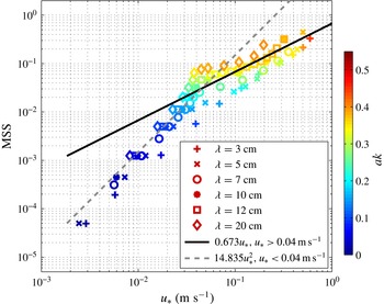
The mean square slope,
 $s_{x}^{2}$
, versus
 $u_{\ast }$
predicted by our model. Note the agreement with the quadratic dependence of (2.27) for small
 $u_{\ast }$
and the change of slope for
 $u_{\ast }>4\times 10^{-2}$
.

3.3. The mean square slope
The
 $x$
component of the mean square slope,
 $s_{x}^{2}$
, is shown as a function of
 $u_{\ast }$
in figure 7. For values of
 $u_{\ast }\leqslant 0.04~\text{m}~\text{s}^{-1}$
,
 $s_{x}^{2}\propto u_{\ast }^{2}$
, consistent with the linear theory of (2.27); however, at larger friction velocities the theory gives results closer to
 $s_{x}^{2}\propto u_{\ast }$
. If we use the drag coefficient measurements of Large & Pond (Reference Large and Pond1981), a friction velocity of
 $0.04~\text{m}~\text{s}^{-1}$
corresponds to
 $U_{10}\approx 1.2~\text{m}~\text{s}^{-1}$
. Thus according to the results in figure 7, for wind speeds above about one metre per second,
 $s_{x}^{2}\propto u_{\ast }$
.
4. Discussion
The primary aim of this work has been to determine whether the viscous dissipation, mainly due to parasitic capillary waves, in a steady solution of pressure-forced gravity–capillary waves of
 $O(1{-}10)$
cm wavelength would be sufficient to balance the wind input at these high wavenumbers in the wind-wave spectrum.
On the basis of the FM98 theory and the wave growth rate data collated by Plant (Reference Plant1982), and the recent numerical modelling by Yang et al. (Reference Yang, Meneveau and Shen2013), the answer is positive within the scatter of the wave growth data, with the dissipation that balances the wave growth showing a clear dependence on wave slope as well as the wave age. The agreement also occurs within a factor of
 $O(1)$
of Miles’ (Reference Miles1959, Reference Miles1993) theories for
 $0.07<u_{\ast }/c<2$
and
 $0.2<ak<0.4$
, when using accepted levels of the Charnock parameter, and within a comparable factor of the results of Yang et al. (Reference Yang, Meneveau and Shen2013) over the available range,
 $0.07<u_{\ast }/c<0.5$
. Given the considerable scatter in the wave growth data, the considerable differences in the wind input models used in numerical wind-wave models (Banner & Morison Reference Banner and Morison2010, figure 3) and the fact that the parasitic capillaries in nature are likely to be unsteady in any frame of reference, it is unlikely that further evidence demonstrating that parasitic capillaries may be the primary wave dissipative mechanism at these high wavenumbers will be achieved without DNS of unsteady wind-forced short waves, and field measurements of gravity–capillary waves. However, the results of this work are, we believe, strong evidence for the dissipative role of the parasitic capillaries on short gravity waves. (Recent DNS of breaking gravity–capillary waves by Deike et al. (Reference Deike, Popinet and Melville2015) are consistent with the dissipation predicted here.)
In reaching the conclusions above, based largely on figure 4, we have plotted
 ${\it\beta}={\it\beta}(u_{\ast }/c)$
, with the slope dependence indicated separately by a colour scale. However, in the FM98 model, all the momentum flux from the air to the water goes into wave growth, whereas in nature only a fraction of the total momentum flux represented by
 $u_{\ast }^{2}$
goes into the waves,
 $u_{\ast w}^{2}$
, with the ratio of the latter to the former given by
 ${\it\chi}\leqslant 1$
. In our comparison of the data with the predictions of FM98,
 ${\it\chi}=1$
. In recent laboratory measurements, Grare et al. (Reference Grare, Peirson, Branger, Walker, Giovangeli and Makin2013, figure 9) find that for
 $0.2<ak<0.35$
, comparable to the range of slopes cited above,
 $0.74<{\it\chi}<1$
. In our solutions, the ratio of the maximum phase speed to the linear phase speed in the range of slopes cited above ranges from
 $1.02<c/c_{0}<1.07$
for
 $3<{\it\lambda}<20~\text{cm}$
. Taking all these effects into account, the comparison of the wave growth data and Miles’ predictions with our predictions of dissipation using the FM98 theory would still balance within a factor of order unity, say an average of 2.2.
In this paper we have used published measurements, Miles’ model of the wind input and recent numerical wind-wave modelling by Yang et al. (Reference Yang, Meneveau and Shen2013) to test whether the dissipation due to parasitic capillary waves may be large enough to balance the wind input to short
 $O(10)$
cm gravity–capillary waves. However, we can also compare the dissipation calculated here against that due to wave breaking. Since
 ${\it\epsilon}_{l}$
is the breaking dissipation per unit length of crest (1.3), the breaking dissipation per unit area for periodic breaking wave trains is just
 ${\dot{E}}_{W}={\it\epsilon}_{l}/{\it\lambda}$
. It follows from (1.3) and (2.17) that
 $$\begin{eqnarray}b={\it\beta}E_{W}g^{\prime }{\it\rho}^{-1}c^{-4}.\end{eqnarray}$$
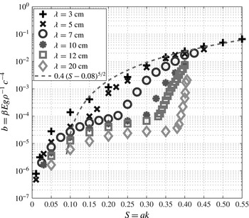
In figure 8 we plot
 $b$
versus
 $ak$
along with the semi-empirical result of Romero et al. (Reference Romero, Melville and Kleiss2012): (1.4), the ‘breaking curve’. For the shorter wavelengths,
 ${\it\lambda}=3$
, 5 and 7 cm, it appears that the breaking curve provides an upper bound on the FM98 dissipation results for
 $ak>0.1$
; with
 ${\it\lambda}=7~\text{cm}$
appearing to approach it asymptotically following the onset of the parasitic capillary effects at
 $ak\approx 0.2$
. For
 ${\it\lambda}=10$
, 12 and 20 cm, with the onset of parasitic capillary effects in the range
 $0.25<ak<0.35$
, there is a rapid increase of
 $b$
approaching the breaking curve, but
 $b$
remains unresolved for
 $ak>0.4$
, the practical limit of our calculations for these longer waves. The results suggest that the semi-empirical relationship for
 $b$
obtained by Romero et al. (Reference Romero, Melville and Kleiss2012) and based on Drazen et al. (Reference Drazen, Melville and Lenain2008) (see also Pizzo & Melville Reference Pizzo and Melville2013) may also prove useful in modelling and bounding the dissipation due to parasitic capillaries (see also Deike et al.
Reference Deike, Popinet and Melville2015).
In view of the simplicity of (2.25), relating the wave growth rate to the wave age and wave slope, it is surprising that, with perhaps the exception of the very recent work by Grare et al. (Reference Grare, Peirson, Branger, Walker, Giovangeli and Makin2013), it has not been previously used to compare with measurements from both the laboratory and the field. (Equation (2.25) in this context arose from a discussion with Laurent Grare regarding an earlier version of Grare et al. (Reference Grare, Peirson, Branger, Walker, Giovangeli and Makin2013) and Townsend (Reference Townsend1972).) The derivation of (2.25) assumes that for weakly nonlinear waves (before the effects of parasitic capillaries become significant) the wave energy density is quadratic in the wave amplitude
 $a$
(Hogan Reference Hogan1980), an assumption that will not be true for very large wave slopes. Thus when plotting
 ${\it\beta}$
over the full range of slopes in the FM98 theory (figure 5), some small departure from (2.25) is seen as
 ${\it\beta}$
ranges over two to three orders of magnitude. The departures from (2.25) are seen in figure 6 and are generally
 $O(ak)$
over the range of wavelengths and slopes studied. It should be noted that the rapid departure at small slopes for the shorter waves is associated with the development of parasitic capillaries at smaller slopes of the shorter waves, and, in the case of 3 cm waves, for which
 $\mathit{Bo}=3.06$
, perhaps due to Wilton’s ripple effects.
The equivalent breaking parameter
 $b$
versus
 $ak$
predicted by the FM98 model. Also shown is the semi-empirical breaking curve
 $b=0.4(ak-0.08)^{5/2}$
of Romero et al. (Reference Romero, Melville and Kleiss2012). Note that above
 $ak=0.1$
, close to the threshold of 0.08, the breaking curve appears to provide an upper bound on
 $b$
, especially for the shorter wavelengths.

We also found that, for the largest slopes we were able to compute for each wavelength, the momentum flux was approximately proportional to the reciprocal of the wavelength, with
 $u_{\ast }^{2}{\it\lambda}=0.023\pm 0.004~\text{m}^{3}~\text{s}^{-1}$
over the six wavelengths considered in this work; thus stressing the importance of the shorter waves in the momentum flux.
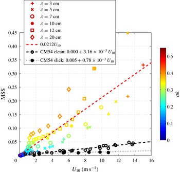
In addition to the dynamics of gravity–capillary waves in equilibrium with the wind forcing, the FM98 theory predicts the statistical description of the idealized steady gravity–capillary wave surface. We had anticipated that the theory would offer some insight into CM54’s field measurements of the correlation between the mean square slope and the wind speed at 10 m,
 $U_{10}$
. Figure 7, which shows the MSS versus
 $u_{\ast }$
, offered some hope when the MSS was approximately proportional to
 $u_{\ast }$
for the larger
 $u_{\ast }$
. However, using a logarithmic atmospheric boundary layer with a simple Charnock relation for the roughness length,
 $$\begin{eqnarray}U(z)=\frac{u_{\ast }}{{\it\kappa}}\ln \left(\frac{z}{z_{0}}\right),\quad z_{0}=\frac{{\it\alpha}_{CH}u_{\ast }^{2}}{g}+\frac{0.11{\it\nu}}{u_{\ast }},\quad {\it\alpha}_{CH}=0.011,\end{eqnarray}$$
to estimate
 $U_{10}$
(Janssen Reference Janssen2004) gave the results shown in figure 9. Here we plot MSS versus
 $U_{10}$
, along with the results of CM54 for the along-wind component of MSS. With significant scatter, our model results give a linear fit to
 $U_{10}$
that is approximately 6.6 times larger than the ‘clean’ surface values of CM54. However, we do not expect the ocean surface to be uniformly distributed with short gravity–capillary waves of the kind modelled here. These
 $O(10)$
cm waves will be generated locally and modulated by the wind and the longer waves as seen in figure 1.
Model predictions of the along-wind component of MSS versus
 $U_{10}$
computed using (4.2), and assuming the entire surface is covered by gravity–capillary waves for each wavelength, along with the CM54 data.

Are the results of figure 9 inconsistent with CM54 and wind-wave dynamics? Now the momentum flux,
 ${\it\rho}_{a}u_{\ast }^{2}$
, is, by definition, momentum per unit time per unit area. Let us assume that, in order to be consistent with the CM54 measurements of MSS, including the fact that the waves of wavenumbers greater than say
 $k_{s}$
contribute a significant fraction of the MSS, the short gravity–capillary waves
 $k>k_{s}$
account for a fraction
 ${\it\alpha}_{s}$
of the total MSS so that longer waves account for
 $(1-{\it\alpha}_{s})$
of the total MSS. Furthermore, the model results show that the MSS for a monochromatic wave representing all
 $k>k_{s}$
would be greater by a factor
 ${\it\gamma}_{s}>1$
than CM54 (cf. figure 9). The implication is that agreement with CM54 on the MSS could be accomplished by the short waves covering a fraction of the surface equal to
 ${\it\alpha}_{s}/{\it\gamma}_{s}$
with an average momentum flux over that area of
 ${\it\rho}_{a}u_{\ast }^{2}$
. The full surface area is covered by the longer waves that are subject now to an average momentum flux
 ${\it\rho}_{a}u_{\ast }^{2}(1-{\it\alpha}_{s}/{\it\gamma}_{s})$
. Thus the total average momentum flux (wind input) to the wave field is still
 ${\it\rho}_{a}u_{\ast }^{2}({\it\alpha}_{s}/{\it\gamma}_{s}+1-{\it\alpha}_{s}/{\it\gamma}_{s})={\it\rho}_{a}u_{\ast }^{2}$
. This and other variants of this simple momentum budget demonstrate that, in the absence of a full wind-wave model, the MSS results of this paper do not fully constrain the dynamics. A full numerical wind-wave model, especially at these higher wavenumbers, would require nonlinear wave–wave interactions, gustiness of the wind, wave modulation and breaking. As far as we are aware, such models typically use the CM54 results to tune the model parameters, with the result that there is no independent prediction of the CM54 results (Munk Reference Munk2009). However, if the equilibrium growth–dissipation regime of these short gravity capillary waves is confirmed by measurements, then the FM98 theory could be used to predict the surface coverage of the high-wavenumber, high-slope wave components consistent with the MSS results of CM54 and potential future measurements.
We expect that the steady solutions, which have been used here to estimate the dissipation in these short gravity–capillary waves, will in nature become unsteady, leading to microbreaking and turbulence. Prompted in part by this work, very recently Deike et al. (Reference Deike, Popinet and Melville2015) have conducted DNS of periodic wave breaking in two dimensions in wave regimes that extend from air-entraining breaking to non-breaking gravity–capillary waves, showing significant agreement with this work, especially in the predictions of the breaking parameter
 $b$
.
It still remains to conduct wind-forced DNS modelling of waves in the gravity–capillary wave range. In anticipation of this possibility, in Fedorov & Melville (Reference Fedorov and Melville2009) we developed a two-layer model of the strongly forced surface layer, with a thin turbulent boundary layer over the underlying irrotational waves. This model leads to instabilities that develop with very steep streamwise gradients in the wave profile, or ‘breaking’, supporting dissipation and mixing in the thin surface layer. Together, these studies suggest the importance of undertaking DNS of these unsteady wind-forced small-scale phenomena, which lie at the heart of an improved understanding of the fluid dynamics of air–sea interaction, air–sea fluxes and their measurement by remote sensing of the ocean surface.
Acknowledgements
We thank Walter Munk for our renewed interest in gravity–capillary waves, which was prompted by discussions about the results of CM54 and Bréon & Henriot (Reference Bréon and Henriot2006). We thank Nick Statom for figure 1, and Ben Reineman for his work on numerous figures, including the final ones that made it into the paper, and Luc Grare for bringing the draft manuscript of Grare et al. (Reference Grare, Peirson, Branger, Walker, Giovangeli and Makin2013) to our attention. We thank Luc Deike for fruitful discussions of numerical simulations of breaking gravity–capillary waves. Professors Shen and Yang kindly made data from Yang et al. (Reference Yang, Meneveau and Shen2013) available. We thank Professor Duncan and three anonymous reviewers whose comments and questions have significantly improved the paper. W.K.M. was supported by grants from the HiRes and RaDyO DRIs at ONR, and from NSF (Physical Oceanography). A.V.F. was supported by the David and Lucile Packard Foundation.