Decomposing the CO2-income tradeoff: an output distance function approach

JON P. REZEK; KEVIN ROGERS

doi:10.1017/S1355770X08004385

Decomposing the CO2-income tradeoff: an output distance function approach

Published online by Cambridge University Press: 01 August 2008

JON P. REZEK and

KEVIN ROGERS

Show author details

JON P. REZEK: Affiliation:
Department of Finance and Economics, Mississippi State University, Box 9590, Mississippi State, MS 39762. Tel: (662) 325-1970. Fax: (662) 325-1977. Email: jrezek@cobilan.msstate.edu
KEVIN ROGERS: Affiliation:
Department of Finance and Economics, Mississippi State University

Article contents

Abstract
Introduction
Model
Empirical estimation
Results
Conclusions
Footnotes
References

Rights & Permissions

Abstract

The environmental Kuznets curve (EKC) hypothesis holds that economic growth leads to increases in pollution in early stages of development, but is a significant driver of environmental improvements as income levels increase. Most empirical applications have focused on estimating a reduced form equation in which the measure of environmental degradation is posited as a non-linear function of income. In this paper we develop a structural production model based on an output distance function to investigate the EKC hypothesis for CO2 in a panel of industrialized countries from 1971 to 2000. This structural approach allows for the decomposition of the observed emission changes into the scale, composition, and productivity effects, thus providing additional insight into the interlinked processes of economic growth and environmental change. The findings from our preferred model indicate that for most countries, the CO2-saving productivity effect is not large enough to offset the CO2-producing scale effect.

Information

Type: Research Article
Information: Environment and Development Economics , Volume 13 , Issue 4 , August 2008 , pp. 457 - 473

DOI: https://doi.org/10.1017/S1355770X08004385 [Opens in a new window]
Copyright: Copyright © Cambridge University Press 2008

1. Introduction

The environmental Kuznets curve (EKC) hypothesis was popularized by the 1992 World Development Report as an explanation of pollution trends observed in much of the developed world. The hypothesis holds that in the early stages of economic development pollution increases along with income, but after countries reach some critical level of development pollution declines even as incomes continue to rise. The important implication of the EKC hypothesis is that environmental degradation is not the inevitable consequence of the development process, but, rather, economic growth can serve as a significant driver of environmental improvements. Indeed, substantial anecdotal evidence and empirical research suggests that pollution and income are not directly and monotonically linked.

A burgeoning literature has emerged testing the validity of the EKC for various pollutants and other measures of environmental degradation.Footnote ¹ Empirical research generally tests for an inverted U-shaped EKC by estimating a reduced form quadratic equation in which the environmental measure serves as the dependent variable and the log of income and income squared enter as explanatory variables. The resulting equation is then used to calculate the income level at which pollution is expected to peak. Researchers have often included additional variables such as income inequality, population density, political measures, and trade openness in their reduced form equations to provide additional explanatory power.

Given the implications for global climate change, the EKC hypothesis is especially germane in the context of carbon dioxide (CO₂) emissions and the various policies designed to reduce them. While many studies point to the existence of an inverted U-shaped EKC for several localized pollutants, no consensus has been reached on pollutants with such global scope. Early research by Holtz-Eakin and Selden (Reference Holtz-Eakin and Seldon1995) and Cole et al. (Reference Cole, Rayner and Bates1997) showed peak per capita CO₂ emissions occurred at per capita income levels of $35,428 and $25,100 respectively for a similar sample of countries. However, these results rely critically on model specification, with upper bounds on the estimates being $8 million and $67,500 respectively.Footnote ²

Recent evidence of an EKC for CO₂ is mixed at best. Using a non-parametric estimator, Bertinelli and Strobl (Reference Bertinelli and Strobl2005) reject the hypothesis of an inverted U-shaped EKC in favor of a monotonically increasing EKC for CO₂ emissions. Friedl and Getzner (Reference Friedl and Getzner2003) find evidence of an N-shaped relation between GDP and CO₂ emissions in Austria. Using a random coefficients model, Cole (Reference Cole2005) shows an EKC which peaks only at extremely high per capita income levels for a restricted set of countries. Galeotti et al. (Reference Galeotti, Lanza and Pauli2006) similarly conclude that the countries sampled affect EKC results. Dijkgraaf and Vollebergh (Reference Dijkgraaf and Vollebergh2005) also challenge the existence of an EKC for CO₂ and express concern about commonly applied cross-country homogeneity assumptions. Stern (Reference Stern2004) suggests that econometric inconsistencies and biased samples may have driven previous EKC results and recommends researchers move beyond reduced form equations which limit the ability of researchers to understand the underlying forces at work, determine their relative magnitudes, and make appropriate policy prescriptions. So while empirical tests of the existence of EKCs for various pollutants may still be of interest, it is illustrative to delve into the structural mechanisms that drive the findings.

The theoretical literature, based mainly on structural models developed by Grossman (Reference Grossman, Goldin and Winters1995) and de Bruyn (Reference de Bruyn1997), highlights three main linkages between pollution and economic activity. The first linkage, the scale effect, implies that an increase in the magnitude of the economy's outputs and inputs will increase pollution commensurately. Individually, this effect is consistent with monotonically increasing emissions. The second linkage, the composition effect, is based on differences in growth rates and emission intensities across an economy's various sectors. Industrialization may increase emissions per unit of output, while an expansion of the tertiary sector is expected to reduce them. Similar changes in an economy's input combination, notably energy usage, will also occur in conjunction with compositional shifts on the output side. However, the composition effect itself cannot lead to infinite reductions in pollution, only to short-run deviations from an upward trend caused by the scale effect.Footnote ³ The final effect, the technology or productivity effect, generally implies that if a clean environment is income elastic, then as incomes increase, society's desire for a cleaner environment manifests itself, through the legislative process and/or pressure from environmental or consumer groups, in the form of cleaner or more efficient production technology. Improved technology allows a country to acquire larger amounts of output even while pollution is reduced. In the long run, it is the productivity effect that drives environmentally sustainable development.

The EKC hypothesis can be explained by the differing magnitudes of these three effects at various levels of development. At low levels of income, a large-scale effect combined with a pollution-producing composition effect may outweigh any minor technology effect, leading to increased pollution as income increases. As incomes continue to grow, however, a muted scale effect may be outweighed by a pollution-saving composition effect and an emergent technology effect, thus lowering emissions. Interaction of these three effects produces the inverted U-shaped EKC, with pollution peaking at some critical per capita income level.

At least two methods are available for investigating the relative magnitudes of the three pollution-income linkages described above. The first method uses an index numbers approach to calculate the various effects by meticulously compiling detailed sectoral data on fuel use and energy and pollution intensities. Unfortunately, such data may not be readily available in many cases. Hamilton and Turton (Reference Hamilton and Turton2002) provide this type of decomposition for CO₂ emissions in nine OECD countries. The second method involves estimation of a global production frontier using linear programming or econometric techniques. The various linkages are then inferred from the estimated production relationships. Stern (Reference Stern2002) uses this type of analysis to decompose sulfur emissions into their proximate causes for a large sample of countries. Zaim and Taskin (Reference Zaim and Taskin2000) and Fare et al. (Reference Färe, Grosskopf, Zaim, Färe and Grosskopf2004) take a similar tack, using data envelopment analysis, a form of non-parametric frontier analysis, to calculate CO₂-adjusted efficiency in OECD countries. However, they do not attempt to decompose these environmental efficiencies into pollution-income linkages.

This paper continues in the frontier analysis vein, using two parametric techniques, deterministic frontier analysis (DFA) and stochastic frontier analysis (SFA), to decompose CO₂ emissions from a panel of OECD countries. The output distance function model we employ has an advantage over the index numbers approach in that it requires less detailed data on emission and energy intensities, which may not be available at the sectoral level. However, its flexibility is also a disadvantage. Since the relationships between inputs and outputs (including CO₂) are estimated internally, the technique generates implied sectoral emission rates and energy intensities that may or may not reflect their true values; however, this technique represents a theoretically valid approach to overcoming the lack of more specific data.

In the next section we model the aggregate production relationship using a multiple-output, multiple-input Shephard output distance function framework. The data and estimation procedures are then described in section 3. The results, presented in section 4, are used to decompose historic changes in CO₂ into their underlying scale, composition and productivity effects. We then use these results to assess the likelihood of the EKC hypothesis for CO₂. Finally, in section 5, we provide brief conclusions.

2. Model

Output distance function

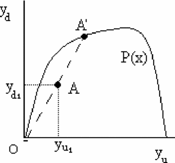
Assume an economy's aggregate production follows a multiple-input, multiple-output process in which a set of x ∈ ℜ^N₊ inputs is transformed into y ∈ ℜ^M₊ outputs. Further, assume that a closed and bounded output set, P(x), encompasses all feasible output bundles. This output set is depicted graphically in figure 1. In such a multi-dimensional context a Shephard (Reference Shephard1970) output distance function provides a convenient framework for representing the production technology. In figure 1, point A represents the observed combination of outputs y ₁ and y ₂ produced from input vector x. The output set P(x) represents the efficiency locus for the given input vector. Points on the P(x) locus are technically efficient, while points in the interior represent an inefficient production combination. The output distance function measures the maximum scalar, θ, by which all output could be expanded and still allow the observation to remain in the feasible set. For observation A this is represented as (OA/OA′).

Figure 1.

Output distance function

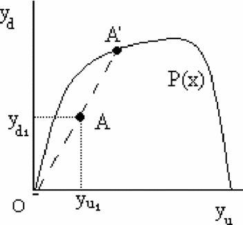
The output distance function is expressed mathematically as

(1)

$\begin{equation} D(x, y)\colon\min\{\theta:y/\theta\in P({\bm x})\}.\end{equation}$

For each observation, the distance function measures the largest feasible radial output expansion, θ, given the current input vector. Observations on the frontier of P(x), have distance function values of unity and are productively efficient. Less efficient observations generate distance function values less than unity, with the result representing the inverse of Farrell's (Reference Farrell1957) output-oriented technical efficiency measure. The primary advantage of an output distance function framework over a simple production function approach in this context is the flexibility it offers for incorporating multiple inputs and outputs, thus contributing to a more complete rendering of the aggregate production relationship. Distance functions have been used extensively in the literature to model multiple-input, multiple-output production processes in the presence of one or more undesirable outputs. Examples include: Coggins and Swinton (Reference Coggins and Swinton1996) for US electricity production, Hailu and Veeman (Reference Hailu and Veeman2000) for Canadian pulp and paper production, Rezek and Perrin (Reference Rezek and Perrin2004) for Great Plains agriculture and Färe et al. (Reference Färe, Grosskopf, Lovell and Yaisawarng1993) for US pulp and paper production. The distance function also provides a mechanism by which the scale, composition, and productivity effects can be disaggregated.

Structural decomposition

As a functional relationship between inputs and outputs, the output distance function can be used to decompose changes in emissions into their constituent components. For ease of exposition, let the output vector y consist of a sub-vector of desirable outputs, y _d, and a single undesirable by-product, y_u. Equation (1) generates an efficiency measure for each observation as given by

(2)

$\begin{equation} \theta = D({\bm y}_{\bm d},y_u,{\bm x},t)\end{equation}$

where y _d = desirable output vector, y_u = undesirable output, x = input vector, and t = technology. Implicitly solving equation (2) for y_u gives an inverse output distance function, with the undesirable by-product specified as a function of the desirable outputs, inputs, technology, and efficiency. The inverse distance function equation is given in general form as

(3)

$\begin{equation} y_u = D({\bm y}_d, x, t, \theta).\end{equation}$

This function describes emission levels in terms of aggregate output production, input usage, the state of technology, and the economy's overall efficiency.

In preparation for empirical decomposition, we take the total differential of equation (3) thus isolating the approximate effects of changes in each of these variables individually. This results in

(4)

$\begin{equation} dy_u = \frac{{\partial D}}{{\partial g}}\,dy_d + \frac{{\partial D}}{{\partial x}}\,dx + \frac{{\partial D}}{{\partial t}}\,dt + \frac{{\partial D}}{{\partial \theta}}\,d\theta\end{equation}$

Using taxonomy similar to Grossman (Reference Grossman, Goldin and Winters1995) we decompose equation (4) into three components, the scale effect, the composition effect, and the productivity effect.

The scale effect refers to the change in emissions resulting from changes in the scale of production, abstracting from any changes caused by substitutions between outputs or between inputs, or changes in technology or efficiency. Mathematically, the scale effect is defined here as

(5)

$\begin{equation} S.E.\equiv\frac{{\partial D}}{{\partial y_d}}\,dy_d^\prime+\frac{{\partial D}}{{\partial x}}\,dx'\end{equation}$

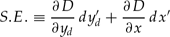
where dy′_d is an equiproportional change in all outputs and dx′ is an equiproportional change in all inputs.

The composition effect demonstrates how emissions change due to the shifting bundle of inputs and outputs, without consideration for changes in the overall scale of economic activity or any efficiency or technical changes in the economy. The composition effect is defined as

(6)

$\begin{equation} C.E. \equiv \left[ {\frac{{\partial D}}{{\partial y_d}}\,dy_d + \frac{{\partial D}}{{\partial x}}\,dx} \right] - \left[ {\frac{{\partial D}}{{\partial y_d}}\,dy_d ^\prime + \frac{{\partial D}}{{\partial x}}\,dx'} \right]\end{equation}$

where dy_d and dx are the observed changes in outputs and inputs respectively. The first bracketed term calculates the change in emissions resulting from actual changes in outputs and inputs, while the second term removes any effects resulting from changes in the scale of production alone. Summing the scale and composition effects yields the first two terms of equation (4).

The third term in equation (4) describes how the undesirable by-product changes as a result of changes in technology, with time serving as a proxy for technological change. The final term in the equation represents the change in emissions resulting from changes in efficiency. While the pure technology effect is well established in the literature, the efficiency component is perhaps overlooked. An important theoretical contribution of the distance function framework in this context is the explicit recognition that emission levels may change due to both technological improvements and changes in productive or environmental efficiency. We combine the pure technology and efficiency components and refer to the joint effect as the productivity effect. This is defined as

(7)

$\begin{equation} P.E.\equiv\frac{{\partial D}}{{\partial t}}\,dt+\frac{{\partial D}}{{\partial \theta}}\,d\theta\end{equation}$

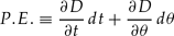
Together, the scale effect, composition effect, and productivity effect constitute a complete decomposition of the emission changes shown in equation (4).

3. Empirical estimation

Data

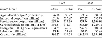
For this analysis we construct a three-input, four-output production model. Data were gathered for a panel of 21 OECD countries from 1971 to 2000. The outputs, gleaned from the World Bank's World Development Indicators 2003 CD-ROM (WDI), are: agricultural output, industrial output, and service sector output, all measured in 1999 (PPP) dollars, and CO₂ emissions measured in tons. Inputs include physical capital stock – gathered from the Penn World Tables (Heston et al., Reference Heston, Summers and Aten2002) and augmented with recent estimates from the Extended Penn World Tables (Marquetti, Reference Marquetti2004) – labor force and commercial energy use – both gathered from the WDI. The descriptive statistics for the first and last years of the sample are shown in table 1.

Table 1.

Descriptive statistics (1971 and 2000)

Note: *1999 PPP dollars.

Deterministic frontier analysis

We first calculate the distance function shown in equation (2) using DFA. With this widely used approach a specific functional form for the distance function is selected and linear programming techniques are used to calculate its parameters in lieu of standard regression analysis. The main advantage of this methodology over the SFA approach described below is that it allows several important properties of the distance function to be readily incorporated into the model using equality and inequality constraints. Specifically, theory requires the output distance function to be non-decreasing in good outputs, non-increasing in inputs, and homogeneous of degree 1 in outputs. Conversely, the drawback to this approach is the lack of a stochastic component – all error is assumed to represent inefficiency. DFA results can therefore be sensitive to data outliers.

For empirical tractability and to ensure a unique solution, we specify two slight variants on a Cobb–Douglas functional form for equation (2) as

(8a)

$\begin{eqnarray} \ln D({\bf x},{\bf y})&=&\alpha_0 +\alpha _1 S + \alpha _2 I + \alpha _3 A + \alpha _4 C + \beta _1 E + \beta _2 L + \beta _3 K + \delta _1 St + \delta _2 It\nonumber\\ &&{+}\,\delta _3 At + \delta _4 Ct + \delta _5 Et + \delta _6 Lt + \delta _7 Kt + \gamma _1 t + \frac{1}{2}\gamma _2 t^2\end{eqnarray}$

and

(8b)

$\begin{eqnarray} \ln D({\bf x},{\bf y}) &=& \alpha _0\,{+}\,\alpha _1 S\,{+}\,\alpha _2 I\,{+}\,\alpha _3 A\,{+}\,\alpha _4 C\,{+}\,\beta _1 E\,{+}\,\beta _2 L\,{+}\,\beta _3 K\,{+}\,\delta _{11} St\nonumber\\ &&{+}\,\delta _{12} St^2\,{+}\,\delta _{21} It\,{+}\,\delta _{22} It^2\,{+}\,\delta _{31} At\,{+}\,\delta _{32} At^2\,{+}\,\delta _{41} Ct\,{+}\,\delta _{42} Ct^2\nonumber\\ &&{+}\,\delta _{51} Et\,{+}\,\delta _{52} Et^2\,{+}\,\delta _{61} Lt\,{+}\,\delta _{62} Lt^2\,{+}\,\delta _{71} Kt\,{+}\,\delta _{72} Kt^2\,{+}\,\gamma _1 t\nonumber\\ &&{+}\,\frac{1}{2}\gamma _2 t^2\,{+}\,\frac{1}{3}\gamma _3 t^3\end{eqnarray}$

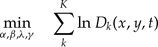
where C= y _u = ln CO₂, S = ln services, I = ln industry, A = ln agriculture, E = ln energy, L = ln labor, K = ln capital, and t = time. Using the Aigner and Chu (Reference Aigner and Chu1968) approach, the GAMS software package is employed to solve the linear program

(9)

$\begin{equation} \mathop{\min}\limits_{\alpha, \beta, \lambda, \gamma} \quad \sum\limits_k^K {\ln D_k} ({x, y, t})\end{equation}$

subject to:

(10)

$\begin{equation} \ln {\rm D}(x, y) \le 0\end{equation}$

(11)

$\begin{equation} \partial \ln D(x, y)/\partial \ln y_d \ge 0\end{equation}$

(12)

$\begin{equation} \partial \ln D(x, y)/\partial \ln x \le 0\end{equation}$

(13)

$\begin{equation} \sum\nolimits_i {\alpha _i = 1}\end{equation}$

(14)

$\begin{equation} \sum\nolimits_i {\delta _i = 0}\end{equation}$

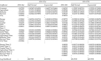
where the panel is T periods in length consisting of K cross-sections. Restriction (10) requires that each observation remain in the feasible set. Equations (11) and (12) ensure that the distance function is non-decreasing in outputs and non-increasing in inputs. Equations (13) and (14) impose homogeneity of degree 1 on outputs. The calculated parameters of the output distance function using DFA are given in columns 2 and 5 of table 2.

Table 2.

Output distance function parameter estimates, DFA and SFA

Note: Standard errors in parentheses for SFA estimates.

Stochastic frontier analysis

We employ the LIMDEP package to estimate the distance function econometrically using SFA. Estimation of equation (2) using SFA poses difficulties since the dependent variable is unobserved; however, the output distance function's homogeneity property can be used to circumvent this obvious shortcoming. Dividing the dependent variable and each of the desirable outputs by the undesirable output imposes homogeneity of degree 1 on outputs. In logs, this transforms equation (2) into

(15)

$\begin{equation} \theta-y_u=D[{({y_d-y_u}),x, t}]\end{equation}$

Rearranging equation (15) gives

(16)

$\begin{equation} - y_u = D[{({y_d - y_u}), x, t}] - \theta\end{equation}$

where θ is now reminiscent of a typical error term.

In SFA, this error term is divided into two components: u, a normally distributed random error term and, v, a one-sided error term representing inefficiency. In this analysis we run two models, one specifies the one-sided error term as following a half-normal distribution and the other an exponential distribution. Applying two variations of the Cobb–Douglas functional form to equation (16), the four-output, three-input model is formulated as

(17a)

$\begin{eqnarray} - C&=&\alpha _0 + \alpha _1 S^* + \alpha _2 I^* + \alpha _3 A^* + \beta _1 E + \beta _2 L + \beta _3 K + \delta _1 S^* t + \delta _2 I^* t + \delta _3 A^* t\nonumber\\ &&{+}\,\delta _4 Et + \delta _5 Lt + \delta _6 Kt + \gamma _1 t + 0.5\gamma _2 t^2 + u + v\end{eqnarray}$

and

(17b)

$\begin{eqnarray} - C &=& \alpha _0 + \alpha _1 S^* + \alpha _2 I^* + \alpha _3 A^* + \beta _1 E + \beta _2 L + \beta _3 K + \delta _{11} S^* t + \delta _{12} S^* t^2\nonumber\\ &&{+}\,\delta _{21} I^* t + \delta _{22} I^* t^2 + \delta _{31} A^* t + \delta _{32} A^* t^2 + \delta _{51} Et + \delta _{52} Et^2 + \delta _{61} Lt\nonumber\\ &&{+}\,\delta _{62} Lt^2 + \delta _{71} Kt + \delta _{72} Kt^2 + \gamma _1 t + \frac{1}{2}\gamma _2 t^2 + \frac{1}{3}\gamma _3 t^3 + u + v\end{eqnarray}$

where S* = ln services – ln CO₂, I* = ln industry – ln CO₂, A* = ln agriculture – ln CO₂, u = normally distributed random error term, and v = one-sided error term (inefficiency). The estimated parameters of equations (17a) and (17b) are given in table 2. Columns 3 and 4 show the results if v is assumed to follow a half-normal distribution and columns 6 and 7 show the results if v is assumed to follow an exponential distribution.

4. Results

Model comparisons

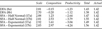
Using the estimated parameters shown in table 2, changes in CO₂ emissions over the sample period are decomposed empirically as specified in equations (5), (6), and (7). To compare across models, the decompositions are depicted in table 3 in terms of the average annual percentage change over the 21 country sample. Column 2 shows that each of the six models is in agreement regarding the scale effect. Carbon dioxide emissions increased by an average of about 2.80 per cent annually from 1971 to 2000 due to increases in overall economic activity.

Table 3.

Model comparisons

Columns 3 and 4 depict the composition and productivity effects, respectively. These effects differ substantially across the DFA and the SFA models. Column 3 shows that, according to the DFA results, changes in economic structure led to a reduction in CO₂ of about 0.15–0.20 per cent per year over the period, but according to the SFA results the composition effect was CO₂-producing, with estimates reaching nearly 3 per cent per year. The productivity effect, shown in column 4, is unambiguously CO₂-saving but its magnitude differs substantially depending on estimation approach and model specification. According to the DFA results, productivity improvements over the period led to an average reduction in CO₂ of about 1.2 per cent annually, but SFA results show productivity improvements reduced CO₂ emissions by much larger amounts, ranging from 2.64 per cent to 4.24 per cent annually. The differences between the DFA and SFA results are driven by the methods used to arrive at the parameters. Specifically, the DFA model explicitly imposes the inequality constraints shown in equations (11) and (12) on the output distance function, but the SFA model does not.Footnote ⁴

Summing columns 2, 3, and 4 of table 3 gives the estimate of the total annual percent change in CO₂ for the panel. The DFA results, especially those calculated from the specification in equation (8a), compare favorably with the actual increase in CO₂ emissions observed during this period (1.42 per cent annually), while the SFA results consistently overestimate CO₂ reduction. This result is not unexpected since the SFA results incorporate a stochastic error component, which necessarily generates a gap between the estimated change in CO₂ and the observed change. Of the four SFA models, the half-normal specification based on equation (17a) provides the best fit in terms of how its decomposition performs in predicting actual emission changes.Footnote ⁵ The country specific analyses in the next sections are therefore based on this model and the DFA model 8a.

DFA results

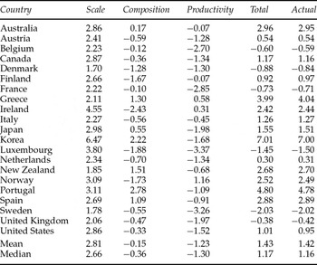
For ease of multilateral comparison, the country-specific DFA results in table 4 are also displayed in terms of average annual percentage change. Column 2 shows the scale effect, which ranged from 1.70 in Denmark and 1.78 in Sweden to 4.55 and 6.47 in rapidly growing Ireland and Korea. The composition effect, depicted in column 3, was pollution-saving in two thirds of the countries in the sample. Ireland reduced emissions by nearly 2.5 per cent per annum due to the shifting structure of its economy, while Korea and Portugal experienced large increases in CO₂ emissions due to composition effects. Finally, the productivity effect generated reductions in CO₂ emissions in 18 countries over the sample period, but this CO₂-saving effect exceeded the CO₂-producing scale effect in only three countries: France, Belgium and Sweden.

Table 4.

Country-specific decomposition of CO₂ emission changes (DFA)

Notes: The decomposition shown in equations (5), (6), and (7) is an approximation, therefore the scale, composition, and productivity effects may not add to observed emission changes.

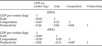
For an inverted U-shaped EKC to develop, the productivity effect (and possibly the composition effect) must initially be smaller than the scale effect, then larger as income grows. It is illustrative, therefore, to investigate the relationship between income and the magnitude of each of the effects. To do this, we calculate the correlations between the initial per capita income levels and the subsequent scale, composition, and productivity effects. The results are depicted for the DFA model in the top panel of table 5. There exists a strong negative correlation between an economy's initial income level and the scale effect experienced over the next 30 years. This implies that higher income economies tend to generate slower growth, and a smaller scale effect, while lower income economies grow more rapidly, generating a larger scale effect. Korea, Ireland, Portugal, and Spain, for example, were all relatively poor countries that produced large amounts of CO₂ through the scale effect due to their rapid ascendancy.

Table 5.

Correlations between initial output per worker and EKC effects

Note: *correlation is significantly different from zero at a 5% level.

There is also a strong negative correlation between initial income level and the composition effect. Those countries beginning at the lower end of the income scale tended to see a shift toward more CO₂-intensive production during the period, exemplified by the positive composition effects. Korea, Greece, Portugal, and Spain are such examples. An interesting exception is Ireland, which, despite starting as a lower income country, experienced a shift toward CO₂-saving production. While many countries recorded negative composition effects, structural changes led to the most substantial reductions in emissions in Ireland and the Scandinavian countries.

The correlation between income and the productivity effect does not appear to be strong. A robust negative correlation here would indicate that productivity change tended to be more CO₂-saving in higher income countries. Such a correlation would support the EKC hypothesis. Of the countries with the largest productivity effects, France, Belgium, and Luxembourg have increased their reliance on nuclear power production and Sweden has shifted toward renewable energy sources. All have moved away from CO₂-intensive coal powered electric plants. Given this observation and the poor correlation results in table 4 it appears that the magnitude of the productivity effect is not related to income but rather to alternative energy production, which tends to have low CO₂ emissions per unit of energy produced. Furthermore, of the countries with productivity effects over 2 per cent, none has significant coal reserves. This result suggests that initial resource endowments play a role in the type of energy sources adopted and hence the magnitude of the productivity effect. Countries with small coal reserves were more likely to exhibit the magnitude of productivity effects necessary to generate an inverted U-shaped EKC. Conversely, countries with larger coal reserves exhibit patterns more consistent with monotonically increasing EKCs. This observation is consistent with Aldy (Reference Aldy2005) who reported in his US state level EKC study that CO₂ emissions were positively related to historic coal endowments.

SFA results

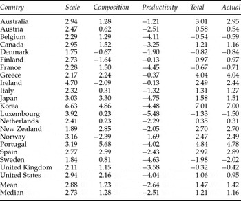
Table 6 presents the SFA decomposition results using the half-normal specification deemed the best fit. The estimated scale effects are similar to the DFA results. Denmark and Sweden exhibited the smallest scale effects and Korea and Ireland again showed exceptionally large-scale effects. Overall, the DFA and SFA scale effects from tables 4 and 6 are highly correlated.

Table 6.

Country-specific decomposition of CO₂ emission changes (SFA)

Note: The decomposition shown in equations (5), (6), and (7) is an approximation, therefore the scale, composition, and productivity effects may not add to observed emission changes.

The SFA composition effect, however, differs from the DFA results. Although the results are highly correlated across countries, the average composition effect is positive and much larger in magnitude, implying that changes in economic structure led to substantial increases in emissions over the period. According to these results, only four countries exhibited a pollution-saving composition effect – Denmark, Norway, Finland, and Ireland. The pollution-producing composition effect was quite large in several countries, generating a 5.6 per cent increase in CO₂ per year in Portugal and a 4.9 per cent increase in Korea. Given the relatively slow pace of sectoral shift in most economies on a year-to-year basis, these results appear disproportionately large.

The estimated DFA and SFA productivity effects are also highly correlated. Like the DFA results, the SFA estimates point to a CO₂-saving productivity effect, but here the effect is much larger, averaging 3.30 per cent over the sample. Luxembourg, Japan, and Sweden were the most successful at advancing the productive frontier in terms of CO₂ reductions, while Norway, Ireland, and Finland lagged. According to these results, the productivity effect was large enough to offset the scale effect in 12 of 21 countries.

Implications for an EKC can be inferred from the correlations on the bottom panel of table 5. As with DFA, both the scale and composition effects are negatively correlated with initial income and the productivity effect is not. This pattern generated poor prospects of an EKC according to the DFA results. However, the SFA results showed that the composition effect was a major driver of emission increases; so, if income is negatively correlated with the composition effect, then economic growth could spur emission reductions, improving the prospects of an inverted U-shaped EKC. However, this interpretation is made with caution since the estimated composition effects appear to be implausibly large.

5. Conclusions

In this paper we develop a theoretical model for decomposing changes in emissions into the constituent scale, composition, and productivity effects. Using an output distance function framework, we then empirically calculate these effects for CO₂ emissions across a panel of OECD countries. Using a deterministic frontier analysis approach, the results indicate that the productivity effect exceeded the scale effect in a few countries, which is consistent with an inverted U-shaped environmental Kuznets curve. However, on average, the productivity and composition effects were not large enough to offset scale effects. This result suggests that reductions in CO₂ emissions, such as those laid out in the Kyoto Protocol or other national policies, are feasible as they have already been achieved in several countries, but must be accompanied by significant technical and environmental efficiency improvements if per capita incomes are to be maintained.

A stochastic frontier analysis approach generates similar results for the scale effect but composition and productivity effects are much different. Contrary to the DFA results, the composition effect was CO₂-producing on average, while the productivity effect produces much larger CO₂-saving effects. Hence, according to the SFA results, emissions are less than they would otherwise be almost solely due to productivity gains. This result is in contrast with the DFA findings, which indicate that in most countries emission savings are generated by both composition and productivity effects.

While there are advantages and disadvantages to each estimation technique, the magnitudes of the three effects appear to be more plausible with the DFA approach. For instance, for the US, the SFA results indicate that productivity improvement reduced CO₂ emissions by about 4 per cent annually, while the DFA model shows the effect was a more reasonable 1.5 per cent per year. Similarly, the SFA results imply changing economic structure increased emissions by over 2 per cent per year, while the DFA results show such changes reduced emission by a more plausible 0.33 per cent per year. Given previous research, it is likely that both changes in the structure of the economy and productivity gains have contributed to CO₂ emission savings.

This research focused mainly on explaining past relationships rather than predicting future emission patterns. Care must be taken to avoid generalizing the results presented here to other economies not included in the analysis. While the DFA approach has the advantage of incorporating the theoretically consistent inequality constraints, it is sensitive to outliers, so inclusion of developing or other economies that are structured much differently from this relatively homogeneous set of OECD countries may produce different results. SFA does not suffer from this potential pitfall, but as we show here, it may generate results that are implausible since constraints consistent with production theory cannot be readily imposed.

Footnotes

¹ See Ekins (Reference Ekins1997), Dasgupta et al. (Reference Dasgupta, Laplante, Wang and Wheeler2002), and Stern (Reference Stern2004) for comprehensive surveys of this literature.

² All figures are in 1990 $US.

³ Furthermore, compositional changes within a country may simply lead to an outsourcing of pollution from developed to industrializing countries, shifting the environmental consequences as described in the pollution haven hypothesis.

⁴ Running the DFA model without restrictions (11) and (12) generates composition effects similar to SFA.

⁵ In terms of the estimated inefficiencies, the chosen SFA results are very similar to the other three SFA models. Correlations of v between the half-normal results of equation (17a) and the other three SFA models range from 92.5 per cent to 96.1 per cent. Choosing one of these four models in isolation would be arbitrary, so we instead examined how closely the four sets of results compared to actual emission changes.

References

Aigner, D.J. and Chu, S.F. 1968, ‘On estimating the industry production function’, American Economic Review 58: 826–839.Google Scholar

Aldy, J.E. 2005, ‘An environmental Kuznets curve analysis of US state-level carbon dioxide emissions’, Journal of Environment and Development 14: 48–72.CrossRef Google Scholar

Bertinelli, L. and Strobl, E. 2005, ‘The environmental Kuznets curve semi-parametrically revisited’, Economics Letters 88: 467–481.CrossRef Google Scholar

Coggins, J.S. and Swinton, J.R. 1996, ‘The price of pollution: a dual approach to valuing SO₂ allowances’, Journal of Environmental Economics and Management 30: 58–72.CrossRef Google Scholar

Cole, M.A. 2005, ‘Re-examining the pollution-income relationship: a random coefficients approach’, Economics Bulletin 14: 1–7.Google Scholar

Cole, M.A., Rayner, A.J., and Bates, J.M 1997, ‘The environmental Kuznets curve: an empirical analysis’, Environment and Development Economics 2: 401–416.CrossRef Google Scholar

Dasgupta, S., Laplante, B., Wang, H., and Wheeler, D. 2002, ‘Confronting the environmental Kuznets curve’, Journal of Economic Perspectives 16: 147–168.CrossRef Google Scholar

de Bruyn, S.M. 1997, ‘Explaining the environmental Kuznets curve: structural change and international agreements in reducing sulphur emissions’, Environment and Development Economics 2: 485–503.CrossRef Google Scholar

Dijkgraaf, E. and Vollebergh, H.R.J. 2005, ‘A test for parameter homogeneity in CO₂ panel EKC estimations’, Environmental and Resource Economics 32: 229–239.CrossRef Google Scholar

Ekins, P. 1997, ‘The Kuznets curve for the environment and economic growth: examining the evidence’, Environment and Planning A 29: 805–830.CrossRef Google Scholar

Färe, R., Grosskopf, S., Lovell, C.A.K., and Yaisawarng, S. 1993, ‘Derivation of shadow prices for undesirable outputs: a distance function approach’, Review of Economics and Statistics 75: 374–380.CrossRef Google Scholar

Färe, R., Grosskopf, S., and Zaim, O. 2004, ‘An environmental Kuznets curve for the OECD countries’, in Färe, R. and Grosskopf, S. (eds), New Directions: Efficiency and Productivity, Dordrecht: Kluwer Adademic Publishers, pp. 77–90.Google Scholar

Farrell, M.J. 1957, ‘The measurement of productive efficiency’, Journal of the Royal Statistical Society 120, Series A, 253–281.CrossRef Google Scholar

Friedl, B. and Getzner, M. 2003, ‘Determinants of CO₂ emissions in a small open economy’, Ecological Economics 45: 133–148.CrossRef Google Scholar

Galeotti, M., Lanza, A., and Pauli, F. 2006, ‘Reassessing the environmental Kuznets curve for CO₂ emissions: a robustness exercise’, Ecological Economics 57: 152–163.CrossRef Google Scholar

Grossman, G.M. 1995, ‘Pollution and growth: what do we know?’, in Goldin, I. and Winters, A.L. (eds), The Economics of Sustainable Development, Cambridge: Cambridge University Press, pp. 19–46.CrossRef Google Scholar

Hailu, A. and Veeman, T.S. 2000, ‘Environmentally sensitive productivity analysis of the Canadian pulp and paper industry, 1959–1994: an input distance function approach’, Journal of Environmental Economics and Management 40: 251–274.CrossRef Google Scholar

Hamilton, C. and Turton, H. 2002, ‘Determinants of emissions growth in OECD countries’, Energy Policy 30: 63–71.CrossRef Google Scholar

Heston, A., Summers, R., and Aten, B. 2002, Penn World Table Version 6.1, Center for International Comparisons at the University of Pennsylvania, October 2002.Google Scholar

Holtz-Eakin, D. and Seldon, T.M. 1995, ‘Stoking the fires? CO₂ emissions and economic growth’, Journal of Public Economics 57: 86–101.CrossRef Google Scholar

Marquetti, A. 2004, Extended Penn World Tables: Economic Growth Data on 118 Countries, !http://homepage.newschool.edu/~foleyd/epwt/.Google Scholar

Rezek, J.P. and Perrin, R.K. 2004, ‘Environmentally adjusted productivity in the Great Plains’, Journal of Agricultural and Resource Economics 29: 346–369.Google Scholar

Shephard, R.W. 1970, Theory of Cost and Production Functions, Princeton, New Jersey: Princeton University Press.Google Scholar

Stern, D.I. 2002, ‘Explaining changes in global sulfur emissions: an econometric decomposition approach’, Ecological Economics 42: 201–220.CrossRef Google Scholar

Stern, D.I. 2004, ‘The rise and fall of the environmental Kuznets curve’, World Development 32: 1419–1439.CrossRef Google Scholar

World Bank 1992, World Bank Development Report 1992: Development and the Environment, Washington, DC: World Bank.Google Scholar

World Bank 2004, World Development Indicators (CD-ROM), Washington, DC: World Bank.Google Scholar

Zaim, O. and Taskin, F. 2000, ‘Environmental efficiency in carbon dioxide emissions in the OECD: a non-parametric approach’, Journal of Environmental Management 58: 95–107.CrossRef Google Scholar