





1 Introduction
This paper is an outgrowth of our attempts, so far incomplete, to develop a real-variable
 $L^{p}$
-theory for two-weight inequalities of the Hilbert transform, which thus far has been achieved in the case
 $p=2$
, by Lacey et al [Reference Lacey4, Reference Lacey, Sawyer, Shen and Uriarte-Tuero5] (see also [Reference Hytönen2]). The search for an
 $L^{p}$
-analogue of certain intermediate results in the existing approach [Reference Lacey4, Reference Lacey, Sawyer, Shen and Uriarte-Tuero5] to the
 $L^{2}$
-theory led us to the present problem which, in our opinion, is natural and interesting in its own right.
The problem we have in mind is that of characterizing the boundedness of a certain positive bilinear form, which is in the spirit of the one appearing in the famous bilinear embedding theorem of Nazarov et al [Reference Nazarov, Treil and Volberg8] and its extension (from
 $L^{2}$
to
 $L^{p}$
) by Lacey et al [Reference Lacey, Sawyer and Uriarte-Tuero6]; these, in turn, are dyadic versions of an old theorem of Sawyer [Reference Sawyer9]. The new feature that distinguishes our problem from those just mentioned is that we want to understand the boundedness not just on
 $L^{p}$
but on
 $L^{p}(\ell ^{2})$
, the space of
 $L^{p}$
functions with values in
 $\ell ^{2}$
or, if the reader prefers, a mixed-norm
 $L^{p}$
space. Recall that such spaces or norms frequently arise in the context of Littlewood–Paley theory and this is also the prospective link of the new bilinear embedding theorem to the sought-after
 $L^{p}$
-theory of the Hilbert transform.
While this link is pure speculation for the time being, our mixed-norm embedding seems independently interesting, both on the level of the result (a Sawyer-type testing, or “local
 $T(1)$
”, characterization) and of the proof. The latter is a non-trivial modification of the successful parallel stopping cubes technology, adapted to the mixed-norm situation; among other things, this extension calls for a new Carleson embedding theorem, proved in §2, which might also have an independent interest.
In order to give a more detailed discussion, we first need to set up some notation.
Fix a dimension
 $n$
of
 $\mathbb{R}^{n}$
. Let
 $\unicode[STIX]{x1D70E}$
and
 $\unicode[STIX]{x1D714}$
be two locally finite non-negative Borel measures in
 $\mathbb{R}^{n}$
. For every real number
 $a\in \mathbb{R}$
let
 $\unicode[STIX]{x1D6FF}_{a}$
denote the Dirac point mass at the point
 $a$
. Using the point masses, we define a measure on
 $(0,\infty )$
by
 $\unicode[STIX]{x1D702}:=\sum _{k\in \mathbb{Z}}\unicode[STIX]{x1D6FF}_{2^{k}}$
. We equip
 $\mathbb{R}_{+}^{n+1}:=\mathbb{R}^{n}\times (0,\infty )$
with the product measure
 $\unicode[STIX]{x1D70E}\times \unicode[STIX]{x1D702}$
.
A
 $\unicode[STIX]{x1D70E}\times \unicode[STIX]{x1D702}$
-measurable function
 $f:\mathbb{R}_{+}^{n+1}\rightarrow \mathbb{C}$
can be identified with the sequence
 $\{f_{k}\}_{k\in \mathbb{Z}}$
of Borel functions defined by
 $f_{k}(x):=f(x,2^{-k})$
. Conversely, a sequence
 $\{f_{k}\}_{k\in \mathbb{Z}}$
of Borel functions on
 $\mathbb{R}^{n}$
can be identified with the
 $\unicode[STIX]{x1D70E}\times \unicode[STIX]{x1D702}$
-measurable function
 $$\begin{eqnarray}f(x,t):=\mathop{\sum }_{k\in \mathbb{Z}}1_{\{2^{-k}\}}(t)f_{k}(x).\end{eqnarray}$$
For a set
 $A\subset \mathbb{R}_{+}^{n+1},A\subset \mathbb{R}^{n}$
or
 $A\subset \mathbb{R}$
, we write
 $1_{A}$
for its characteristic function.
Let
 $p\in [1,\infty )$
. For a
 $\unicode[STIX]{x1D70E}\times \unicode[STIX]{x1D702}$
-measurable function
 $f$
, we write
 $$\begin{eqnarray}\Vert f\Vert _{L^{p}(\unicode[STIX]{x1D70E};\!\ell ^{2})}:=\biggl(\int _{\mathbb{R}^{n}}\biggl(\mathop{\sum }_{k\in \mathbb{Z}}|f_{k}(x)|^{2}\biggr)^{p/2}\,\,\mathit{d}\unicode[STIX]{x1D70E}(x)\biggr)^{1/p},\end{eqnarray}$$
and the space
 $L^{p}(\unicode[STIX]{x1D70E};\!\ell ^{2})$
is defined to be the set of those
 $f$
such that (1.1) is finite. If
 $f$
is a
 $\unicode[STIX]{x1D70E}\times \unicode[STIX]{x1D702}$
-measurable function, we write
 $$\begin{eqnarray}|f|_{\ell ^{2}}(x):=\biggl(\mathop{\sum }_{k\in \mathbb{Z}}|f_{k}(x)|^{2}\biggr)^{1/2},\quad x\in \mathbb{R}^{n}.\end{eqnarray}$$
For any Borel function
 $g$
on
 $\mathbb{R}^{n}$
, we define
 $$\begin{eqnarray}\Vert g\Vert _{L^{p}(\unicode[STIX]{x1D714})}:=\biggl(\int _{\mathbb{R}^{n}}|g(x)|^{p}\,\,\mathit{d}\unicode[STIX]{x1D714}\biggr)^{1/p}.\end{eqnarray}$$
The space
 $L^{p}(\unicode[STIX]{x1D714})$
is the set of those
 $g$
such that (1.2) is finite. Using the measure
 $\unicode[STIX]{x1D70E}$
we define similarly
 $\Vert g\Vert _{L^{p}(\unicode[STIX]{x1D70E})}$
and the space
 $L^{p}(\unicode[STIX]{x1D70E})$
.
Let
 $\mathscr{D}$
be the dyadic lattice
 $$\begin{eqnarray}\mathscr{D}:=\{2^{-k}([0,1)^{n}+m):k\in \mathbb{Z},m\in \mathbb{Z}^{n}\}.\end{eqnarray}$$
For every
 $Q\in \mathscr{D}$
denote by
 $\widehat{Q}$
the Carleson box
 $Q\times (0,\ell (Q)]$
, where
 $\ell (Q)$
is the side length of the cube
 $Q$
. Let
 $\unicode[STIX]{x1D707}$
be a fixed non-negative
 $\unicode[STIX]{x1D70E}\times \unicode[STIX]{x1D702}$
-measurable function and suppose that for each dyadic cube
 $Q\in \mathscr{D}$
there is associated a non-negative real number
 $\unicode[STIX]{x1D706}_{Q}$
.
If
 $f:\mathbb{R}_{+}^{n+1}\rightarrow [0,\infty )$
is
 $\unicode[STIX]{x1D70E}\times \unicode[STIX]{x1D702}$
-measurable and
 $g:\mathbb{R}^{n}\rightarrow [0,\infty )$
is a Borel function, we define
 $$\begin{eqnarray}\unicode[STIX]{x1D6EC}(f,g):=\mathop{\sum }_{Q\in \mathscr{D}}\unicode[STIX]{x1D706}_{Q}\iint _{\widehat{Q}}f\unicode[STIX]{x1D707}\,\,\mathit{d}\unicode[STIX]{x1D702}\,\mathit{d}\unicode[STIX]{x1D70E}\int _{Q}g\,\mathit{d}\unicode[STIX]{x1D714},\end{eqnarray}$$
and also for every
 $Q_{0}\in \mathscr{D}$
the localized version
 $$\begin{eqnarray}\unicode[STIX]{x1D6EC}_{Q_{0}}(f,g):=\mathop{\sum }_{\substack{ Q\in \mathscr{D} \\ Q\subset Q_{0}}}\unicode[STIX]{x1D706}_{Q}\iint _{\widehat{Q}}f\unicode[STIX]{x1D707}\,\mathit{d}\unicode[STIX]{x1D702}\,\mathit{d}\unicode[STIX]{x1D70E}\int _{Q}g\,\mathit{d}\unicode[STIX]{x1D714}.\end{eqnarray}$$
The problem we are considering is when there exists a constant
 $C$
such that the inequality
 $$\begin{eqnarray}\unicode[STIX]{x1D6EC}(f,g)\leqslant C\Vert f\Vert _{L^{p}(\unicode[STIX]{x1D70E};\ell ^{2})}\Vert g\Vert _{L^{p^{\prime }}(\unicode[STIX]{x1D714})}\end{eqnarray}$$
holds for all non-negative
 $f$
and
 $g$
, where
 $p\in (1,\infty )$
and
 $p^{\prime }$
is the Hölder conjugate of
 $p$
. We emphasize that we consider the function
 $\unicode[STIX]{x1D707}$
and the coefficients
 $\{\unicode[STIX]{x1D706}_{Q}\}_{Q\in \mathscr{D}}$
related to the definition of
 $\unicode[STIX]{x1D6EC}$
as fixed here. If such a constant
 $C$
exists then we may define
 $\unicode[STIX]{x1D6EC}(f,g)$
for every
 $f\in L^{p}(\unicode[STIX]{x1D70E};\ell ^{2})$
and
 $g\in L^{p^{\prime }}(\unicode[STIX]{x1D714})$
by (1.3) and (1.4) continues to hold for these functions. Note that we could rephrase this problem equivalently by asking whether the operator
 $$\begin{eqnarray}T^{\unicode[STIX]{x1D70E}}f:=\mathop{\sum }_{Q\in \mathscr{D}}\unicode[STIX]{x1D706}_{Q}\iint _{\widehat{Q}}f\unicode[STIX]{x1D707}\,\,\mathit{d}\unicode[STIX]{x1D702}\,\mathit{d}\unicode[STIX]{x1D70E}1_{Q}\end{eqnarray}$$
is bounded from
 $L^{p}(\unicode[STIX]{x1D70E};\ell ^{2})$
into
 $L^{p}(\unicode[STIX]{x1D714})$
.
If (1.4) holds, then
 $\Vert 1_{\widehat{Q}}\unicode[STIX]{x1D707}\Vert _{L^{p^{\prime }}(\unicode[STIX]{x1D70E};\ell ^{2})}<\infty$
for every
 $Q\in \mathscr{D}$
such that
 $\unicode[STIX]{x1D706}_{Q},\unicode[STIX]{x1D70E}(Q)$
and
 $\unicode[STIX]{x1D714}(Q)$
are non-zero. Therefore, without changing the problem, we may assume that
 $$\begin{eqnarray}\Vert 1_{\widehat{Q}}\unicode[STIX]{x1D707}\Vert _{L^{p^{\prime }}(\unicode[STIX]{x1D70E};\ell ^{2})}<\infty ,\quad \text{for every }Q\in \mathscr{D}.\end{eqnarray}$$
We answer this question when
 $p\geqslant 2$
in terms of a testing characterization, i.e., we show that to have the inequality (1.4) it is enough to test it with a certain class of test functions. To get a precise meaning for this we state our main theorem.
Theorem 1.1. Let
 $p\in [2,\infty )$
. For every
 $Q\in \mathscr{D}$
define the function
 $$\begin{eqnarray}\unicode[STIX]{x1D711}_{Q}:=|1_{\widehat{Q}}\unicode[STIX]{x1D707}|_{\ell ^{2}}^{p^{\prime }-2}1_{\widehat{Q}}\unicode[STIX]{x1D707},\end{eqnarray}$$
that satisfies
 $\Vert \unicode[STIX]{x1D711}_{Q}\Vert _{L^{p}(\unicode[STIX]{x1D70E};\ell ^{2})}<\infty$
by (1.5).
Let
 ${\mathcal{T}}$
and
 ${\mathcal{T}}^{\ast }$
denote the smallest possible constants, with the understanding that they may be
 $\infty$
, such that
 $$\begin{eqnarray}\unicode[STIX]{x1D6EC}_{Q}(\unicode[STIX]{x1D711}_{Q},g)\leqslant {\mathcal{T}}\Vert \unicode[STIX]{x1D711}_{Q}\Vert _{L^{p}(\unicode[STIX]{x1D70E};\ell ^{2})}\Vert g\Vert _{L^{p^{\prime }}(\unicode[STIX]{x1D714})}\end{eqnarray}$$
and
 $$\begin{eqnarray}\unicode[STIX]{x1D6EC}_{Q}(f,1_{Q})\leqslant {\mathcal{T}}^{\ast }\Vert f\Vert _{L^{p}(\unicode[STIX]{x1D70E};\ell ^{2})}\Vert 1_{Q}\Vert _{L^{p^{\prime }}(\unicode[STIX]{x1D714})}\end{eqnarray}$$
hold for every
 $Q\in \mathscr{D}$
and every non-negative
 $\unicode[STIX]{x1D70E}\times \unicode[STIX]{x1D702}$
-measurable function
 $f$
and non-negative Borel function
 $g$
. Then there exists a constant
 $C<\infty$
such that (1.4) holds if and only if
 ${\mathcal{T}}+{\mathcal{T}}^{\ast }<\infty$
. Moreover, if
 ${\mathcal{T}}+{\mathcal{T}}^{\ast }<\infty$
, the smallest possible constant
 $\Vert \unicode[STIX]{x1D6EC}\Vert$
in (1.4) satisfies
 $$\begin{eqnarray}\Vert \unicode[STIX]{x1D6EC}\Vert \simeq {\mathcal{T}}+{\mathcal{T}}^{\ast }.\end{eqnarray}$$
To prove Theorem 1.1 we use, as already mentioned, the method of parallel stopping cubes. This technique was first introduced by Lacey et al [Reference Lacey, Sawyer, Shen and Uriarte-Tuero5] in an earlier arXiv version of their work, but replaced by other tools in the published paper. In [Reference Hytönen3] the parallel stopping cubes were used to study a similar problem but with usual
 $L^{p}$
norms rather than mixed ones. Our approach was to follow the outline of the proof in [Reference Hytönen3], but in the set-up of this paper, it is not clear in the beginning what should be the class of test functions in (1.7). However, if one assumes that there exists a family
 $\{\unicode[STIX]{x1D711}_{Q}\}_{Q\in \mathscr{D}}$
of test functions on
 $\mathbb{R}_{+}^{n+1}$
and starts to follow the outline of [Reference Hytönen3], then there comes a situation that allows one to guess the test functions, which leads to the definition (1.6). Then it turns out that these test functions are of the right form to conclude the proof. We show in the end of §3 how one can arrive at the definition (1.6).
The case
 $p=2$
in Theorem 1.1 reduces to easier techniques. In fact, it can be seen as a special case of the result in [Reference Nazarov, Treil and Volberg8]. The case
 $p\in (1,2)$
is an open problem, that we discuss more in §4, where we also state our conjecture about the two-weight inequality of the Hilbert transform in
 $L^{p}$
.
For two numbers
 $\unicode[STIX]{x1D6FC},\unicode[STIX]{x1D6FD}\geqslant 0$
we use the notation
 $\unicode[STIX]{x1D6FC}\lesssim \unicode[STIX]{x1D6FD}$
to mean that there exists an absolute constant
 $C$
such that
 $\unicode[STIX]{x1D6FC}\leqslant C\unicode[STIX]{x1D6FD}$
. Sometimes we write for example
 $\unicode[STIX]{x1D6FC}{\lesssim}_{p}\unicode[STIX]{x1D6FD}$
to indicate that the implicit constant depends on
 $p$
. Two sided estimates
 $\unicode[STIX]{x1D6FC}\lesssim \unicode[STIX]{x1D6FD}\lesssim \unicode[STIX]{x1D6FC}$
are abbreviated as
 $\unicode[STIX]{x1D6FC}\simeq \unicode[STIX]{x1D6FD}$
.
2 An embedding theorem
In this section we start collecting tools to prove the main theorem, Theorem 1.1. In particular, we prove a Carleson-type embedding theorem that arises naturally during the proof in the next section.
We begin with a lemma that is the reason why we need to have
 $p\geqslant 2$
in Theorem 1.1.
Lemma 2.1. Let
 $p\geqslant 2$
. Suppose
 $\{E_{i}\}_{i\in {\mathcal{I}}}$
is a countable collection of
 $\unicode[STIX]{x1D70E}\times \unicode[STIX]{x1D702}$
-measurable sets such that
 $E_{i}\cap E_{j}=\emptyset$
if
 $i\not =j$
. Let
 $f$
be a non-negative
 $\unicode[STIX]{x1D70E}\times \unicode[STIX]{x1D702}$
-measurable function. Then
 $$\begin{eqnarray}\mathop{\sum }_{i\in {\mathcal{I}}}\Vert 1_{E_{i}}f\Vert _{L^{p}(\unicode[STIX]{x1D70E};\ell ^{2})}^{p}\leqslant \Vert f\Vert _{L^{p}(\unicode[STIX]{x1D70E};\ell ^{2})}^{p}.\end{eqnarray}$$
Proof. Since
 $p/2\geqslant 1$
, we have
 $$\begin{eqnarray}\displaystyle \phantom{\hspace{14.39996pt}}\mathop{\sum }_{i\in {\mathcal{I}}}\Vert 1_{E_{i}}f\Vert _{L^{p}(\unicode[STIX]{x1D70E};\ell ^{2})}^{p} & = & \displaystyle \int _{\mathbb{R}^{n}}\mathop{\sum }_{i\in {\mathcal{I}}}\biggl(\mathop{\sum }_{k\in \mathbb{Z}}1_{E_{i}}(x,2^{k})f(x,2^{k})^{2}\biggr)^{p/2}\,\mathit{d}\unicode[STIX]{x1D70E}(x)\nonumber\\ \displaystyle & {\leqslant} & \displaystyle \int _{\mathbb{R}^{n}}\biggl(\mathop{\sum }_{i\in {\mathcal{I}}}\mathop{\sum }_{k\in \mathbb{Z}}1_{E_{i}}(x,2^{k})f(x,2^{k})^{2}\biggr)^{p/2}\,\mathit{d}\unicode[STIX]{x1D70E}(x)\nonumber\\ \displaystyle & {\leqslant} & \displaystyle \Vert f\Vert _{L^{p}(\unicode[STIX]{x1D70E};\ell ^{2})}^{p}.\phantom{\hspace{147.60004pt}}\square\nonumber\end{eqnarray}$$
Next we state the well-known dyadic Carleson embedding theorem that will be applied later. Let
 $\unicode[STIX]{x1D708}$
be a locally finite non-negative Borel measure in
 $\mathbb{R}^{n}$
and suppose
 $\{a_{Q}\}_{Q\in \mathscr{D}}$
is a collection of non-negative real numbers. We write the average over
 $Q\in \mathscr{D}$
of a Borel function
 $h:\mathbb{R}^{n}\rightarrow [0,\infty )$
as
 $\langle h\rangle _{Q}^{\unicode[STIX]{x1D708}}:=\unicode[STIX]{x1D708}(Q)^{-1}\int _{Q}h\,\mathit{d}\unicode[STIX]{x1D708}$
, that is understood to be zero if
 $\unicode[STIX]{x1D708}(Q)=0$
. Let
 $p\in (1,\infty )$
. There exists a constant
 $C$
such that
 $$\begin{eqnarray}\mathop{\sum }_{Q\in \mathscr{D}}(\langle h\rangle _{Q}^{\unicode[STIX]{x1D708}})^{p}a_{Q}\leqslant C\int _{\mathbb{R}^{n}}h^{p}\,\mathit{d}\unicode[STIX]{x1D708}\end{eqnarray}$$
holds for all Borel functions
 $h:\mathbb{R}^{n}\rightarrow [0,\infty )$
if and only if there exists a constant
 $C^{\prime }$
such that
 $$\begin{eqnarray}\mathop{\sum }_{\substack{ Q^{\prime }\in \mathscr{D} \\ Q^{\prime }\subset Q}}a_{Q^{\prime }}\leqslant C^{\prime }\unicode[STIX]{x1D708}(Q)\end{eqnarray}$$
holds for all
 $Q\in \mathscr{D}$
. Moreover, the smallest possible constants in (2.1) and (2.2) satisfy
 $C\simeq _{p}C^{\prime }$
.
Stopping cubes
Here we show how to construct the collections of stopping cubes relevant to the present purposes. Let
 $Q_{0}\in \mathscr{D}$
and let
 $g:\mathbb{R}^{n}\rightarrow [0,\infty )$
be a locally
 $\unicode[STIX]{x1D714}$
-integrable function. Set
 $\mathscr{G}_{0}:=\{Q_{0}\}$
and suppose that the collections
 $\mathscr{G}_{j},j\in \{0,1,\ldots ,k\}$
, are defined for some
 $k$
. If
 $G\in \mathscr{G}_{k}$
, we define
 $\text{ch}_{\mathscr{G}}(G)$
to be the collection of maximal dyadic cubes
 $Q\in \mathscr{D}$
such that
 $Q\subset G$
and
 $\langle g\rangle _{Q}^{\unicode[STIX]{x1D714}}>2\langle g\rangle _{G}^{\unicode[STIX]{x1D714}}.$
Then we set
 $\mathscr{G}_{k+1}:=\bigcup _{G\in \mathscr{G}_{k}}\text{ch}_{\mathscr{G}}(G)$
and the collection of stopping cubes with the top cube
 $Q_{0}$
is defined as
 $\mathscr{G}:=\bigcup _{k=0}^{\infty }\mathscr{G}_{k}$
.
If
 $Q\in \mathscr{D},Q\subset Q_{0},$
we denote by
 $\unicode[STIX]{x1D70B}_{\mathscr{G}}(Q)$
the smallest cube
 $G\in \mathscr{G}$
that contains
 $Q$
. From the definition of
 $\mathscr{G}$
it is seen that
 $$\begin{eqnarray}\langle g\rangle _{Q}^{\unicode[STIX]{x1D714}}\leqslant 2\langle g\rangle _{\unicode[STIX]{x1D70B}_{\mathscr{ G}}(Q)}^{\unicode[STIX]{x1D714}}.\end{eqnarray}$$
It follows from the construction that
 $\mathscr{G}$
is a 2-Carleson family (with respect to
 $\unicode[STIX]{x1D714}$
), which means that for every
 $G\in \mathscr{G}$
there holds
 $$\begin{eqnarray}\mathop{\sum }_{\substack{ G^{\prime }\in \mathscr{G} \\ G^{\prime }\subset G}}\unicode[STIX]{x1D714}(G^{\prime })\leqslant 2\unicode[STIX]{x1D714}(G).\end{eqnarray}$$
This combined with the dyadic Carleson embedding theorem stated above implies that
 $$\begin{eqnarray}\mathop{\sum }_{G\in \mathscr{G}}(\langle h\rangle _{G}^{\unicode[STIX]{x1D714}})^{p}\unicode[STIX]{x1D714}(G){\lesssim}_{p}\int h^{p}\,\mathit{d}\unicode[STIX]{x1D714}\end{eqnarray}$$
holds for every Borel function
 $h:\mathbb{R}^{n}\rightarrow [0,\infty )$
and every
 $p\in (1,\infty )$
.
Let
 $f:\mathbb{R}_{+}^{n+1}\rightarrow [0,\infty )$
be a
 $\unicode[STIX]{x1D70E}\times \unicode[STIX]{x1D702}$
-measurable function such that
 $$\begin{eqnarray}\iint _{\widehat{Q_{0}}}f\unicode[STIX]{x1D707}\,\mathit{d}\unicode[STIX]{x1D702}\,\mathit{d}\unicode[STIX]{x1D70E}<\infty ,\end{eqnarray}$$
where again
 $Q_{0}\in \mathscr{D}$
is some fixed cube. We want to define a similar collection of cubes for the function
 $f$
involving the test functions
 $\unicode[STIX]{x1D711}_{Q}$
from (1.6). The reason why we define the collection as follows becomes more apparent when one studies what happens in the equations (3.7) and (3.8) below in the proof of the main theorem. First set
 $\mathscr{F}_{0}:=\{Q_{0}\}$
and suppose
 $\mathscr{F}_{0},\ldots ,\mathscr{F}_{k}$
are defined for some
 $k$
. Let
 $F\in \mathscr{F}_{k}$
. We define
 $\text{ch}_{\mathscr{F}}(F)$
to be the set of maximal cubes
 $Q\in \mathscr{D}$
such that
 $Q\subset F$
and
 $$\begin{eqnarray}\frac{\iint _{\widehat{Q}}f\unicode[STIX]{x1D707}\,\mathit{d}\unicode[STIX]{x1D702}\,\mathit{d}\unicode[STIX]{x1D70E}}{\iint _{\widehat{Q}}\unicode[STIX]{x1D711}_{F}\unicode[STIX]{x1D707}\,\mathit{d}\unicode[STIX]{x1D702}\,\mathit{d}\unicode[STIX]{x1D70E}}>A\frac{\iint _{\widehat{F}}f\unicode[STIX]{x1D707}\,\mathit{d}\unicode[STIX]{x1D702}\,\mathit{d}\unicode[STIX]{x1D70E}}{\iint _{\widehat{F}}\unicode[STIX]{x1D711}_{F}\unicode[STIX]{x1D707}\,\mathit{d}\unicode[STIX]{x1D702}\,\mathit{d}\unicode[STIX]{x1D70E}},\end{eqnarray}$$
where
 $A>0$
is a big enough constant to be specified during the proof of the main theorem in §3. Then
 $\mathscr{F}_{k+1}:=\bigcup _{F\in \mathscr{F}_{k}}\text{ch}_{\mathscr{F}}(F)$
and the collection of stopping cubes for
 $f$
with the top cube
 $Q_{0}$
is
 $\mathscr{F}:=\bigcup _{k=0}^{\infty }\mathscr{F}_{k}$
.
If
 $Q\in \mathscr{D},Q\subset Q_{0}$
, we denote by
 $\unicode[STIX]{x1D70B}_{\mathscr{F}}(Q)$
the smallest cube
 $F\in \mathscr{F}$
that contains
 $Q$
. It follows from the construction of
 $\mathscr{F}$
that
 $$\begin{eqnarray}\frac{\iint _{\widehat{Q}}f\unicode[STIX]{x1D707}\,\mathit{d}\unicode[STIX]{x1D702}\,\mathit{d}\unicode[STIX]{x1D70E}}{\iint _{\widehat{Q}}\unicode[STIX]{x1D711}_{F}\unicode[STIX]{x1D707}\,\mathit{d}\unicode[STIX]{x1D702}\,\mathit{d}\unicode[STIX]{x1D70E}}\leqslant A\frac{\iint _{\widehat{F}}f\unicode[STIX]{x1D707}\,\mathit{d}\unicode[STIX]{x1D702}\,\mathit{d}\unicode[STIX]{x1D70E}}{\iint _{\widehat{F}}\unicode[STIX]{x1D711}_{F}\unicode[STIX]{x1D707}\,\mathit{d}\unicode[STIX]{x1D702}\,\mathit{d}\unicode[STIX]{x1D70E}},\quad F=\unicode[STIX]{x1D70B}_{\mathscr{F}}(Q).\end{eqnarray}$$
Related to these define for
 $Q\in \mathscr{D}$
the average-type quantity
 $$\begin{eqnarray}[f]_{Q}:=\frac{\iint _{\widehat{Q}}f\unicode[STIX]{x1D707}\,\mathit{d}\unicode[STIX]{x1D702}\,\mathit{d}\unicode[STIX]{x1D70E}}{\iint _{\widehat{Q}}\unicode[STIX]{x1D711}_{Q}\unicode[STIX]{x1D707}\,\mathit{d}\unicode[STIX]{x1D702}\,\mathit{d}\unicode[STIX]{x1D70E}}.\end{eqnarray}$$
For later use we record here a few identities related to the test functions
 $\unicode[STIX]{x1D711}_{Q}$
. Namely, a direct computation shows that
 $$\begin{eqnarray}\iint _{\widehat{Q}}\unicode[STIX]{x1D711}_{Q}\unicode[STIX]{x1D707}\,\mathit{d}\unicode[STIX]{x1D702}\,\mathit{d}\unicode[STIX]{x1D70E}=\int _{Q}|1_{\widehat{Q}}\unicode[STIX]{x1D707}|_{\ell ^{2}}^{p^{\prime }}\,\mathit{d}\unicode[STIX]{x1D70E}=\Vert 1_{\widehat{Q}}\unicode[STIX]{x1D707}\Vert _{L^{p^{\prime }}(\unicode[STIX]{x1D70E};\ell ^{2})}^{p^{\prime }}=\Vert \unicode[STIX]{x1D711}_{Q}\Vert _{L^{p}(\unicode[STIX]{x1D70E};\ell ^{2})}^{p}.\end{eqnarray}$$
Now we are ready for the embedding theorem that is the main result of this section.
Proposition 2.2. Let
 $p\in [2,\infty )$
and
 $Q_{0}\in \mathscr{D}$
. Let
 $f:\mathbb{R}_{+}^{n+1}\rightarrow [0,\infty )$
be a
 $\unicode[STIX]{x1D70E}\times \unicode[STIX]{x1D702}$
-measurable function such that
 $$\begin{eqnarray}\iint _{\widehat{Q_{0}}}f\unicode[STIX]{x1D707}\,\mathit{d}\unicode[STIX]{x1D702}\,\mathit{d}\unicode[STIX]{x1D70E}<\infty .\end{eqnarray}$$
Let
 $\mathscr{F}$
be the collection stopping cubes for the function
 $f$
with the top cube
 $Q_{0}$
as described above. Then
 $$\begin{eqnarray}\mathop{\sum }_{F\in \mathscr{F}}[f]_{F}^{p}\Vert \unicode[STIX]{x1D711}_{F}\Vert _{L^{p}(\unicode[STIX]{x1D70E};\ell ^{2})}^{p}{\lesssim}_{p}\Vert f\Vert _{L^{p}(\unicode[STIX]{x1D70E};\ell ^{2})}^{p}.\end{eqnarray}$$
It is important to note that here we need the fact
 $p\geqslant 2$
, because in the proof we apply Lemma 2.1 that does not hold for
 $p\in (1,2)$
.
Inequality (2.8) somewhat resembles Inequality (2.1) and we shall actually interpret the left-hand side of (2.8) in a way that allows us to apply the dyadic Carleson embedding theorem.
Proof of Proposition 2.2.
Our first goal is to show that for every
 $F\in \mathscr{F}$
there holds
 $$\begin{eqnarray}\mathop{\sum }_{\substack{ F^{\prime }\in \text{ch}_{\mathscr{ F}}(F)}}\Vert \unicode[STIX]{x1D711}_{F^{\prime }}\Vert _{L^{p}(\unicode[STIX]{x1D70E};\ell ^{2})}^{p}\leqslant \frac{1}{2}\Vert \unicode[STIX]{x1D711}_{F}\Vert _{L^{p}(\unicode[STIX]{x1D70E};\ell ^{2})}^{p}\end{eqnarray}$$
if the parameter
 $A$
related to the construction of
 $\mathscr{F}$
is big enough. Recall the identity
 $\Vert \unicode[STIX]{x1D711}_{Q}\Vert _{L^{p}(\unicode[STIX]{x1D70E};\ell ^{2})}^{p}=\int _{Q}|1_{\widehat{Q}}\unicode[STIX]{x1D707}|_{\ell ^{2}}^{p^{\prime }}\,\mathit{d}\unicode[STIX]{x1D70E}.$
Fix a cube
 $F\in \mathscr{F}$
and define
 $$\begin{eqnarray}H:=\biggl\{x\in F:|1_{\widehat{F}}\unicode[STIX]{x1D707}|_{\ell ^{2}}(x)>B\mathop{\sum }_{F^{\prime }\in \text{ch}_{\mathscr{ F}}(F)}|1_{\widehat{F^{\prime }}}\unicode[STIX]{x1D707}|_{\ell ^{2}}(x)\biggr\},\end{eqnarray}$$
where
 $B>0$
is a big constant that will be fixed soon. Then there holds
 $$\begin{eqnarray}\displaystyle \mathop{\sum }_{F^{\prime }\in \text{ch}_{\mathscr{ F}}(F)}\int _{F^{\prime }\cap H}|1_{\widehat{F^{\prime }}}\unicode[STIX]{x1D707}|_{\ell ^{2}}^{p^{\prime }}\,\mathit{d}\unicode[STIX]{x1D70E} & {\leqslant} & \displaystyle \mathop{\sum }_{F^{\prime }\in \text{ch}_{\mathscr{ F}}(F)}B^{-p^{\prime }}\int _{F^{\prime }\cap H}|1_{\widehat{F}}\unicode[STIX]{x1D707}|_{\ell ^{2}}^{p^{\prime }}\,\mathit{d}\unicode[STIX]{x1D70E}\nonumber\\ \displaystyle & {\leqslant} & \displaystyle B^{-p^{\prime }}\int _{F}|1_{\widehat{F}}\unicode[STIX]{x1D707}|_{\ell ^{2}}^{p^{\prime }}\,\mathit{d}\unicode[STIX]{x1D70E},\end{eqnarray}$$
since the cubes
 $F^{\prime }\in \text{ch}_{\mathscr{F}}(F)$
are pairwise disjoint.
On the other hand, because
 $p^{\prime }-2\leqslant 0$
, we can estimate in
 $F^{\prime }\setminus H$
, where
 $F^{\prime }\in \text{ch}_{\mathscr{F}}(F)$
, that
 $$\begin{eqnarray}\displaystyle \int _{F^{\prime }\setminus H}|1_{\widehat{F^{\prime }}}\unicode[STIX]{x1D707}|_{\ell ^{2}}^{p^{\prime }}\,\mathit{d}\unicode[STIX]{x1D70E} & = & \displaystyle \int _{F^{\prime }\setminus H}|1_{\widehat{F^{\prime }}}\unicode[STIX]{x1D707}|_{\ell ^{2}}^{p^{\prime }-2}|1_{\widehat{F^{\prime }}}\unicode[STIX]{x1D707}|_{\ell ^{2}}^{2}\,\mathit{d}\unicode[STIX]{x1D70E}\nonumber\\ \displaystyle & {\leqslant} & \displaystyle B^{2-p^{\prime }}\int _{F^{\prime }\setminus H}|1_{\widehat{F}}\unicode[STIX]{x1D707}|_{\ell ^{2}}^{p^{\prime }-2}|1_{\widehat{F^{\prime }}}\unicode[STIX]{x1D707}|_{\ell ^{2}}^{2}\,\mathit{d}\unicode[STIX]{x1D70E}\nonumber\\ \displaystyle & {\leqslant} & \displaystyle B^{2-p^{\prime }}\iint _{\widehat{F^{\prime }}}\unicode[STIX]{x1D711}_{F}\unicode[STIX]{x1D707}\,\mathit{d}\unicode[STIX]{x1D702}\,\mathit{d}\unicode[STIX]{x1D70E}.\nonumber\end{eqnarray}$$
Hence, the stopping condition (2.4) gives
 $$\begin{eqnarray}\displaystyle \mathop{\sum }_{F^{\prime }\in \text{ch}_{\mathscr{ F}}(F)}\int _{F^{\prime }\setminus H}|1_{\widehat{F^{\prime }}}\unicode[STIX]{x1D707}|_{\ell ^{2}}^{p^{\prime }}\,\mathit{d}\unicode[STIX]{x1D70E} & {\leqslant} & \displaystyle B^{2-p^{\prime }}\mathop{\sum }_{F^{\prime }\in \text{ch}_{\mathscr{ F}}(F)}\iint _{\widehat{F^{\prime }}}\unicode[STIX]{x1D711}_{F}\unicode[STIX]{x1D707}\,\mathit{d}\unicode[STIX]{x1D702}\,\mathit{d}\unicode[STIX]{x1D70E}\nonumber\\ \displaystyle & {\leqslant} & \displaystyle B^{2-p^{\prime }}A^{-1}\frac{\iint _{\widehat{F}}\unicode[STIX]{x1D711}_{F}\unicode[STIX]{x1D707}\,\mathit{d}\unicode[STIX]{x1D702}\,\mathit{d}\unicode[STIX]{x1D70E}}{\iint _{\widehat{F}}f\unicode[STIX]{x1D707}\,\mathit{d}\unicode[STIX]{x1D702}\,\mathit{d}\unicode[STIX]{x1D70E}}\nonumber\\ \displaystyle & & \displaystyle \times \,\mathop{\sum }_{F^{\prime }\in \text{ch}_{\mathscr{ F}}(F)}\iint _{\widehat{F^{\prime }}}f\unicode[STIX]{x1D707}\,\mathit{d}\unicode[STIX]{x1D702}\,\mathit{d}\unicode[STIX]{x1D70E}\nonumber\\ \displaystyle & {\leqslant} & \displaystyle B^{2-p^{\prime }}A^{-1}\iint _{\widehat{F}}\unicode[STIX]{x1D711}_{F}\unicode[STIX]{x1D707}\,\mathit{d}\unicode[STIX]{x1D702}\,\mathit{d}\unicode[STIX]{x1D70E}\nonumber\\ \displaystyle & = & \displaystyle B^{2-p^{\prime }}A^{-1}\int _{F}|1_{\widehat{F}}\unicode[STIX]{x1D707}|_{\ell ^{2}}^{p^{\prime }}\,\mathit{d}\unicode[STIX]{x1D70E}.\end{eqnarray}$$
Combining estimates (2.10) and (2.11) with the identity
 $\Vert \unicode[STIX]{x1D711}_{F}\Vert _{L^{p}(\unicode[STIX]{x1D70E};\ell ^{2})}^{p}=\int _{F}|1_{\widehat{F}}\unicode[STIX]{x1D707}|^{p^{\prime }}\,\mathit{d}\unicode[STIX]{x1D70E}$
we have
 $$\begin{eqnarray}\mathop{\sum }_{F^{\prime }\in \text{ch}_{\mathscr{ F}}(F)}\Vert \unicode[STIX]{x1D711}_{F^{\prime }}\Vert _{L^{p}(\unicode[STIX]{x1D70E};\ell ^{2})}^{p}\leqslant (B^{-p^{\prime }}+B^{2-p^{\prime }}A^{-1})\Vert \unicode[STIX]{x1D711}_{F}\Vert _{L^{p}(\unicode[STIX]{x1D70E};\ell ^{2})}^{p}.\end{eqnarray}$$
From here it is seen that if we choose for example
 $B:=4^{1/p^{\prime }}$
and
 $A:=4B^{2-p^{\prime }}$
, then (2.9) is satisfied. By summing a geometric series, from (2.9) it follows that
 $$\begin{eqnarray}\mathop{\sum }_{\substack{ F^{\prime }\in \mathscr{F} \\ F^{\prime }\subset F}}\Vert \unicode[STIX]{x1D711}_{F^{\prime }}\Vert _{L^{p}(\unicode[STIX]{x1D70E};\ell ^{2})}^{p}\leqslant 2\Vert \unicode[STIX]{x1D711}_{F}\Vert _{L^{p}(\unicode[STIX]{x1D70E};\ell ^{2})}^{p}\end{eqnarray}$$
holds for every
 $F\in \mathscr{F}$
.
Next we view the sum
 $\sum _{F\in \mathscr{F}}[f]_{F}^{p}\Vert \unicode[STIX]{x1D711}_{F}\Vert _{L^{p}(\unicode[STIX]{x1D70E};\ell ^{2})}^{p}$
in a way that allows us to apply the dyadic Carleson embedding theorem. If
 $F\in \mathscr{F}$
, we write
 $$\begin{eqnarray}E_{\mathscr{F}}(\widehat{F}):=\widehat{F}\bigg\backslash\mathop{\bigcup }_{F^{\prime }\in \text{ch}_{\mathscr{ F}}(F)}\widehat{F^{\prime }}.\end{eqnarray}$$
Note that the sets
 $E_{\mathscr{F}}(\widehat{F})$
are pairwise disjoint. Moreover, there holds
 $$\begin{eqnarray}\widehat{F}=\mathop{\bigcup }_{\substack{ F^{\prime }\in \mathscr{F} \\ F^{\prime }\subset F}}E_{\mathscr{F}}(\widehat{F}^{\prime })\end{eqnarray}$$
for every
 $F\in \mathscr{F}$
.
Define a measure
 $\unicode[STIX]{x1D708}$
on
 $\mathbb{R}^{n+1}$
by
 $$\begin{eqnarray}\unicode[STIX]{x1D708}:=\mathop{\sum }_{F\in \mathscr{F}}\Vert \unicode[STIX]{x1D711}_{F}\Vert _{L^{p}(\unicode[STIX]{x1D70E};\ell ^{2})}^{p}\unicode[STIX]{x1D6FF}_{z(F)},\qquad z(F):=(\text{centre}(F),{\textstyle \frac{3}{4}}\ell (F)),\end{eqnarray}$$
where
 $\text{centre}(F)$
is the centre of the
 $n$
-dimensional cube
 $F$
and
 $z(F)$
is the centre of the upper-half of the
 $(n+1)$
-dimensional cube
 $\widehat{F}$
. Define also a function
 $\unicode[STIX]{x1D6FC}$
on
 $\mathbb{R}^{n+1}$
by
 $$\begin{eqnarray}\unicode[STIX]{x1D6FC}:=\mathop{\sum }_{F\in \mathscr{F}}\frac{\iint _{E_{\mathscr{F}}(\widehat{F})}f\unicode[STIX]{x1D707}\,\mathit{d}\unicode[STIX]{x1D702}\,\mathit{d}\unicode[STIX]{x1D70E}}{\Vert \unicode[STIX]{x1D711}_{F}\Vert _{L^{p}(\unicode[STIX]{x1D70E};\ell ^{2})}^{p}}1_{\{z(F)\}},\end{eqnarray}$$
and recall that
 $\iint _{\widehat{F}}\unicode[STIX]{x1D711}_{F}\unicode[STIX]{x1D707}\,\mathit{d}\unicode[STIX]{x1D702}\,\mathit{d}\unicode[STIX]{x1D70E}=\Vert \unicode[STIX]{x1D711}_{F}\Vert _{L^{p}(\unicode[STIX]{x1D70E};\ell ^{2})}^{p}$
by equation (2.7).
Let
 $F\in \mathscr{F}$
. Then, by (2.12), there holds that
 $$\begin{eqnarray}\unicode[STIX]{x1D708}(\widehat{F})=\mathop{\sum }_{\substack{ F^{\prime }\in \mathscr{F} \\ F^{\prime }\subset F}}\Vert \unicode[STIX]{x1D711}_{F^{\prime }}\Vert _{L^{p}(\unicode[STIX]{x1D70E};\ell ^{2})}^{p}\simeq \Vert \unicode[STIX]{x1D711}_{F}\Vert _{L^{p}(\unicode[STIX]{x1D70E};\ell ^{2})}^{p},\end{eqnarray}$$
and thus also
 $$\begin{eqnarray}\mathop{\sum }_{\substack{ F^{\prime }\in \mathscr{F} \\ F^{\prime }\subset F}}\unicode[STIX]{x1D708}(\widehat{F^{\prime }})\simeq \mathop{\sum }_{\substack{ F^{\prime }\in \mathscr{F} \\ F^{\prime }\subset F}}\Vert \unicode[STIX]{x1D711}_{F^{\prime }}\Vert _{L^{p}(\unicode[STIX]{x1D70E};\ell ^{2})}^{p}=\unicode[STIX]{x1D708}(\widehat{F}).\end{eqnarray}$$
This says that the collection
 $\widehat{\mathscr{F}}:=\{\widehat{F}:F\in \mathscr{F}\}$
is a Carleson family with respect to the measure
 $\unicode[STIX]{x1D708}$
.
Note that for every
 $F\in \mathscr{F}$
we have
 $$\begin{eqnarray}\iint _{\widehat{F}}f\unicode[STIX]{x1D707}\,\mathit{d}\unicode[STIX]{x1D702}\,\mathit{d}\unicode[STIX]{x1D70E}=\mathop{\sum }_{\substack{ F^{\prime }\in \mathscr{F} \\ F^{\prime }\subset F}}\frac{\iint _{E_{\mathscr{F}}(\widehat{F^{\prime }})}f\unicode[STIX]{x1D707}\,\mathit{d}\unicode[STIX]{x1D702}\,\mathit{d}\unicode[STIX]{x1D70E}}{\Vert \unicode[STIX]{x1D711}_{F^{\prime }}\Vert _{L^{p}(\unicode[STIX]{x1D70E};\ell ^{2})}^{p}}\Vert \unicode[STIX]{x1D711}_{F^{\prime }}\Vert _{L^{p}(\unicode[STIX]{x1D70E};\ell ^{2})}^{p}=\int _{\widehat{F}}\unicode[STIX]{x1D6FC}\,\mathit{d}\unicode[STIX]{x1D708},\end{eqnarray}$$
and, hence,
 $$\begin{eqnarray}[f]_{F}^{p}\Vert \unicode[STIX]{x1D711}_{F}\Vert _{L^{p}(\unicode[STIX]{x1D70E};\ell ^{2})}^{p}=\biggl(\frac{\iint _{\widehat{F}}f\unicode[STIX]{x1D707}\,\mathit{d}\unicode[STIX]{x1D702}\,\mathit{d}\unicode[STIX]{x1D70E}}{\Vert \unicode[STIX]{x1D711}_{F}\Vert _{L^{p}(\unicode[STIX]{x1D70E};\ell ^{2})}^{p}}\biggr)^{p}\Vert \unicode[STIX]{x1D711}_{F}\Vert _{L^{p}(\unicode[STIX]{x1D70E};\ell ^{2})}^{p}\simeq \biggl(\frac{\int _{\widehat{F}}\unicode[STIX]{x1D6FC}\,\mathit{d}\unicode[STIX]{x1D708}}{\unicode[STIX]{x1D708}(\widehat{F})}\biggr)^{p}\unicode[STIX]{x1D708}(\widehat{F}).\end{eqnarray}$$
We can now apply the dyadic Carleson embedding theorem to conclude that
 $$\begin{eqnarray}\mathop{\sum }_{F\in \mathscr{F}}[f]_{F}^{p}\Vert \unicode[STIX]{x1D711}_{F}\Vert _{L^{p}(\unicode[STIX]{x1D70E};\ell ^{2})}^{p}\simeq \mathop{\sum }_{F\in \mathscr{F}}\biggl(\frac{\int _{\widehat{F}}\unicode[STIX]{x1D6FC}\,\mathit{d}\unicode[STIX]{x1D708}}{\unicode[STIX]{x1D708}(\widehat{F})}\biggr)^{p}\unicode[STIX]{x1D708}(\widehat{F})\lesssim \int _{\mathbb{ R}^{n+1}}\unicode[STIX]{x1D6FC}^{p}\,\mathit{d}\unicode[STIX]{x1D708}.\end{eqnarray}$$
Writing out the definition of
 $\unicode[STIX]{x1D6FC}$
and
 $\unicode[STIX]{x1D708}$
we have
 $$\begin{eqnarray}\displaystyle \int _{\mathbb{R}^{n+1}}\unicode[STIX]{x1D6FC}^{p}\,\mathit{d}\unicode[STIX]{x1D708} & = & \displaystyle \mathop{\sum }_{F\in \mathscr{F}}\biggl(\frac{\iint _{E_{\mathscr{F}}(\widehat{F})}f\unicode[STIX]{x1D707}\,\mathit{d}\unicode[STIX]{x1D702}\,\mathit{d}\unicode[STIX]{x1D70E}}{\Vert \unicode[STIX]{x1D711}_{F}\Vert _{L^{p}(\unicode[STIX]{x1D70E};\ell ^{2})}^{p}}\biggr)^{p}\Vert \unicode[STIX]{x1D711}_{F}\Vert _{L^{p}(\unicode[STIX]{x1D70E};\ell ^{2})}^{p}\nonumber\\ \displaystyle & {\leqslant} & \displaystyle \mathop{\sum }_{F\in \mathscr{F}}\biggl(\frac{\Vert 1_{E_{\mathscr{F}}(\widehat{F})}f\Vert _{L^{p}(\unicode[STIX]{x1D70E};\ell ^{2})}\Vert 1_{\widehat{F}}\unicode[STIX]{x1D707}\Vert _{L^{p^{\prime }}(\unicode[STIX]{x1D70E};\ell ^{2})}}{\Vert \unicode[STIX]{x1D711}_{F}\Vert _{L^{p}(\unicode[STIX]{x1D70E};\ell ^{2})}^{p}}\biggr)^{p}\Vert \unicode[STIX]{x1D711}_{F}\Vert _{L^{p}(\unicode[STIX]{x1D70E};\ell ^{2})}^{p}\nonumber\\ \displaystyle & = & \displaystyle \mathop{\sum }_{F\in \mathscr{F}}\Vert 1_{E_{\mathscr{F}}(\widehat{F})}f\Vert _{L^{p}(\unicode[STIX]{x1D70E};\ell ^{2})}^{p}\leqslant \Vert f\Vert _{L^{p}(\unicode[STIX]{x1D70E};\ell ^{2})}^{p},\nonumber\end{eqnarray}$$
where we used the identity
 $\Vert \unicode[STIX]{x1D711}_{F}\Vert _{L^{p}(\unicode[STIX]{x1D70E};\ell ^{2})}^{p}=\Vert 1_{\widehat{F}}\unicode[STIX]{x1D707}\Vert _{L^{p^{\prime }}(\unicode[STIX]{x1D70E};\ell ^{2})}^{p^{\prime }}$
and applied Lemma 2.1. This concludes the proof.◻
3 Proof of Theorem 1.1
In this section we prove Theorem 1.1. After the proof we show how one can arrive at the definition (1.6) of the test functions
 $\unicode[STIX]{x1D711}_{Q}$
.
Proof of Theorem 1.1.
If (1.4) holds, then it is clear that the testing conditions (1.7) and (1.8) hold, and that
 $\max ({\mathcal{T}},{\mathcal{T}}^{\ast })\leqslant \Vert \unicode[STIX]{x1D6EC}\Vert$
. Hence, we can focus on the converse, that is, we assume that
 ${\mathcal{T}},{\mathcal{T}}^{\ast }<\infty$
and show that
 $\Vert \unicode[STIX]{x1D6EC}\Vert \lesssim {\mathcal{T}}+{\mathcal{T}}^{\ast }$
. By monotonicity it is enough to fix an arbitrary cube
 $Q_{0}\in \mathscr{D}$
and two non-negative functions
 $f\in L^{p}(\unicode[STIX]{x1D70E};\ell ^{2})$
and
 $g\in L^{p^{\prime }}(\unicode[STIX]{x1D714})$
and to show that
 $$\begin{eqnarray}\mathop{\sum }_{\substack{ Q\in \mathscr{D} \\ Q\subset Q_{0}}}\unicode[STIX]{x1D706}_{Q}\iint _{\widehat{Q}}f\unicode[STIX]{x1D707}\,\mathit{d}\unicode[STIX]{x1D702}\,\mathit{d}\unicode[STIX]{x1D70E}\int _{Q}g\,\mathit{d}\unicode[STIX]{x1D714}\lesssim ({\mathcal{T}}+{\mathcal{T}}^{\ast })\Vert f\Vert _{L^{p}(\unicode[STIX]{x1D70E};\ell ^{2})}\Vert g\Vert _{L^{p^{\prime }}(\unicode[STIX]{x1D714})}.\end{eqnarray}$$
Let
 $\mathscr{F}$
and
 $\mathscr{G}$
be the collections of stopping cubes for the functions
 $f$
and
 $g$
, respectively, with the top cube
 $Q_{0}$
as described in §2. Using
 $\mathscr{F}$
and
 $\mathscr{G}$
we can reorganize the sum in the left-hand side of (3.1). If
 $Q\in \mathscr{F},Q\subset Q_{0}$
, then there exists a unique pair
 $(F,G)\in \mathscr{F}\times \mathscr{G}$
, denoted by
 $\unicode[STIX]{x1D70B}(Q)$
, such that
 $\unicode[STIX]{x1D70B}_{\mathscr{F}}(Q)=F$
and
 $\unicode[STIX]{x1D70B}_{\mathscr{G}}(Q)=G$
. Since in this case clearly
 $F\cap G\not =\emptyset$
, it follows from the properties of dyadic cubes that either
 $F\subset G$
or
 $G\subset F$
. Hence, it is seen that the left-hand side of (3.1) satisfies
 $$\begin{eqnarray}\text{LHS}\text{(3.1)}=\mathop{\sum }_{F\in \mathscr{F}}\mathop{\sum }_{\substack{ G\in \mathscr{G} \\ G\subset F}}\mathop{\sum }_{\substack{ Q\in \mathscr{D} \\ \unicode[STIX]{x1D70B}(Q)=(F,G)}}+\mathop{\sum }_{G\in \mathscr{G}}\mathop{\sum }_{\substack{ F\in \mathscr{F} \\ F\subsetneq G}}\mathop{\sum }_{\substack{ Q\in \mathscr{D} \\ \unicode[STIX]{x1D70B}(Q)=(F,G)}}=:I+\mathit{II}.\end{eqnarray}$$
The proof divides into considering the parts
 $I$
and
 $\mathit{II}$
separately.
Estimate for II
For
 $G\in \mathscr{G}$
define the collection
 $$\begin{eqnarray}\text{ch}_{\mathscr{G}}^{\ast }(G):=\{G^{\prime }\in \text{ch}_{\mathscr{ G}}(G):\unicode[STIX]{x1D70B}_{\mathscr{F}}(G^{\prime })\subset G\}.\end{eqnarray}$$
Also, write
 $E_{\mathscr{G}}(\widehat{G}):=\widehat{G}\setminus \bigcup _{G^{\prime }\in \text{ch}_{\mathscr{ G}}(G)}\widehat{G^{\prime }}$
.
Let
 $Q\in \mathscr{D},F\in \mathscr{F}$
and
 $G\in \mathscr{G}$
be such that
 $F\subsetneq G$
and
 $\unicode[STIX]{x1D70B}(Q)=(F,G)$
. Note first that
 $$\begin{eqnarray}\widehat{G}=E_{\mathscr{G}}(\widehat{G})\cup \mathop{\bigcup }_{G^{\prime }\in \text{ch}_{\mathscr{ G}}(G)}\widehat{G^{\prime }}.\end{eqnarray}$$
Because
 $Q\subset G$
, and accordingly
 $\widehat{Q}\subset \widehat{G}$
, this implies that
 $$\begin{eqnarray}\widehat{Q}=(E_{\mathscr{G}}(\widehat{G})\cap \widehat{Q})\cup \mathop{\bigcup }_{\substack{ G^{\prime }\in \text{ch}_{\mathscr{ G}}(G)}}(\widehat{G^{\prime }}\cap \widehat{Q}).\end{eqnarray}$$
Let
 $G^{\prime }\in \text{ch}_{\mathscr{G}}(G)$
. If
 $G^{\prime }\cap Q=\emptyset$
, then clearly
 $\widehat{G^{\prime }}\cap \widehat{Q}=\emptyset$
. Assume
 $G^{\prime }\cap Q\not =\emptyset$
. Then, since
 $\unicode[STIX]{x1D70B}_{\mathscr{G}}(Q)=G$
, it must be that
 $G^{\prime }\subsetneq Q$
. Also, since
 $G^{\prime }\subsetneq Q\subset F\subsetneq G$
, we can conclude that
 $G^{\prime }\in \text{ch}_{\mathscr{G}}^{\ast }(G)$
. This reasoning shows that actually
 $$\begin{eqnarray}\widehat{Q}=(E_{\mathscr{G}}(\widehat{G})\cap \widehat{Q})\cup \mathop{\bigcup }_{\substack{ G^{\prime }\in \text{ch}_{\mathscr{ G}}^{\ast }(G) \\ G^{\prime }\subsetneq Q}}\widehat{G^{\prime }},\end{eqnarray}$$
where one should note that the sets
 $E_{\mathscr{G}}(\widehat{G})$
and
 $\widehat{G^{\prime }}$
,
 $G^{\prime }\in \text{ch}_{\mathscr{G}}(G)$
, are pairwise disjoint.
If
 $Q\in \mathscr{D},F\in \mathscr{F}$
and
 $G\in \mathscr{G}$
are such that
 $F\subsetneq G$
and
 $\unicode[STIX]{x1D70B}(Q)=(F,G)$
, we can write in view of (3.2) that
 $$\begin{eqnarray}\iint _{\widehat{Q}}f\unicode[STIX]{x1D707}\,\mathit{d}\unicode[STIX]{x1D702}\,\mathit{d}\unicode[STIX]{x1D70E}=\iint _{\widehat{Q}}f_{G}\unicode[STIX]{x1D707}\,\mathit{d}\unicode[STIX]{x1D702}\,\mathit{d}\unicode[STIX]{x1D70E},\end{eqnarray}$$
where
 $$\begin{eqnarray}f_{G}:=1_{E_{\mathscr{G}}(\widehat{G})}f+\mathop{\sum }_{\substack{ G^{\prime }\in \text{ch}_{\mathscr{ G}}^{\ast }(G)}}\frac{\iint _{\widehat{G^{\prime }}}f\unicode[STIX]{x1D707}\,\mathit{d}\unicode[STIX]{x1D70E}}{\iint _{\widehat{G^{\prime }}}\unicode[STIX]{x1D711}_{\unicode[STIX]{x1D70B}_{\mathscr{F}}(G^{\prime })}\unicode[STIX]{x1D707}\,\mathit{d}\unicode[STIX]{x1D70E}}1_{\widehat{G^{\prime }}}\unicode[STIX]{x1D711}_{\unicode[STIX]{x1D70B}_{\mathscr{F}}(G^{\prime })}.\end{eqnarray}$$
Hence,
 $$\begin{eqnarray}\displaystyle \mathit{II} & {\leqslant} & \displaystyle 2\mathop{\sum }_{G\in \mathscr{G}}\langle g\rangle _{G}^{\unicode[STIX]{x1D714}}\mathop{\sum }_{\substack{ F\in \mathscr{F} \\ F\subsetneq G}}\mathop{\sum }_{\substack{ Q\in \mathscr{D} \\ \unicode[STIX]{x1D70B}(Q)=(F,G)}}\unicode[STIX]{x1D706}_{Q}\iint _{\widehat{Q}}f_{G}\unicode[STIX]{x1D707}\,\mathit{d}\unicode[STIX]{x1D702}\,\mathit{d}\unicode[STIX]{x1D70E}\int _{Q}1_{G}\,\mathit{d}\unicode[STIX]{x1D714}\nonumber\\ \displaystyle & {\leqslant} & \displaystyle 2\mathop{\sum }_{G\in \mathscr{G}}\langle g\rangle _{G}^{\unicode[STIX]{x1D714}}\unicode[STIX]{x1D6EC}_{G}(f_{G},1_{G})\leqslant 2{\mathcal{T}}^{\ast }\mathop{\sum }_{G\in \mathscr{G}}\langle g\rangle _{G}^{\unicode[STIX]{x1D714}}\Vert f_{G}\Vert _{L^{p}(\unicode[STIX]{x1D70E};\ell ^{2})}\unicode[STIX]{x1D714}(G)^{1/p^{\prime }}\nonumber\\ \displaystyle & {\leqslant} & \displaystyle 2{\mathcal{T}}^{\ast }\biggl(\mathop{\sum }_{G\in \mathscr{G}}\Vert f_{G}\Vert _{L^{p}(\unicode[STIX]{x1D70E};~\!\ell ^{2})}^{p}\biggr)^{1/p}\biggl(\mathop{\sum }_{G\in \mathscr{G}}(\langle g\rangle _{G}^{\unicode[STIX]{x1D714}})^{p^{\prime }}\unicode[STIX]{x1D714}(G)\biggr)^{1/p^{\prime }}.\end{eqnarray}$$
Equation (2.3) gives that
 $$\begin{eqnarray}\biggl(\mathop{\sum }_{G\in \mathscr{G}}(\langle g\rangle _{G}^{\unicode[STIX]{x1D714}})^{p^{\prime }}\unicode[STIX]{x1D714}(G)\biggr)^{1/p^{\prime }}\lesssim \Vert g\Vert _{L^{p^{\prime }}(\unicode[STIX]{x1D714})}.\end{eqnarray}$$
Fix some
 $G\in \mathscr{G}$
. We have
 $$\begin{eqnarray}\displaystyle \Vert f_{G}\Vert _{L^{p}(\unicode[STIX]{x1D70E};\ell ^{2})} & {\leqslant} & \displaystyle \Vert 1_{E_{\mathscr{G}}(\widehat{G})}f\Vert _{L^{p}(\unicode[STIX]{x1D70E};\ell ^{2})}\nonumber\\ \displaystyle & & \displaystyle +\biggl\|\mathop{\sum }_{\substack{ G^{\prime }\in \text{ch}_{\mathscr{ G}}^{\ast }(G)}}\frac{\iint _{\widehat{G^{\prime }}}f\unicode[STIX]{x1D707}\,\mathit{d}\unicode[STIX]{x1D70E}}{\iint _{\widehat{G^{\prime }}}\unicode[STIX]{x1D711}_{\unicode[STIX]{x1D70B}_{\mathscr{F}}(G^{\prime })}\unicode[STIX]{x1D707}\,\mathit{d}\unicode[STIX]{x1D70E}}1_{\widehat{G^{\prime }}}\unicode[STIX]{x1D711}_{\unicode[STIX]{x1D70B}_{\mathscr{F}}(G^{\prime })}\biggr\|_{L^{p}(\unicode[STIX]{x1D70E};\ell ^{2})}.\nonumber\end{eqnarray}$$
For every
 $G^{\prime }\in \text{ch}_{\mathscr{G}}^{\ast }(G)$
there exists a cube
 $F\in \mathscr{F}$
such that
 $G^{\prime }\subset F\subset G$
and
 $\unicode[STIX]{x1D70B}_{\mathscr{F}}(G^{\prime })=F$
, whence it follows that
 $\unicode[STIX]{x1D70B}_{\mathscr{G}}(F)=G$
or
 $F\in \text{ch}_{\mathscr{G}}(G)$
. Hence, the sum over
 $G^{\prime }\in \text{ch}_{\mathscr{G}}^{\ast }(G)$
can be written as
 $$\begin{eqnarray}\mathop{\sum }_{G^{\prime }\in \text{ch}_{\mathscr{ G}}^{\ast }(G)}=\mathop{\sum }_{\substack{ F\in \mathscr{F}: \\ \unicode[STIX]{x1D70B}_{\mathscr{G}}(F)=G\text{ or} \\ F\in \text{ch}_{\mathscr{G}}(G)}}\mathop{\sum }_{\substack{ G^{\prime }\in \text{ch}_{\mathscr{ G}}(G) \\ \unicode[STIX]{x1D70B}_{\mathscr{F}}(G^{\prime })=F}}.\end{eqnarray}$$
Also, the stopping condition implies for
 $G^{\prime }\in \text{ch}_{\mathscr{G}}^{\ast }(G)$
that
 $$\begin{eqnarray}\frac{\iint _{\widehat{G^{\prime }}}f\unicode[STIX]{x1D707}\,\mathit{d}\unicode[STIX]{x1D70E}}{\iint _{\widehat{G^{\prime }}}\unicode[STIX]{x1D711}_{\unicode[STIX]{x1D70B}_{\mathscr{F}}(G^{\prime })}\unicode[STIX]{x1D707}\,\mathit{d}\unicode[STIX]{x1D70E}}\leqslant A[f]_{\unicode[STIX]{x1D70B}_{\mathscr{F}}(G^{\prime })}.\end{eqnarray}$$
Since the cubes
 $G^{\prime }\in \text{ch}_{\mathscr{G}}^{\ast }(G)$
are pairwise disjoint, (3.5) and (3.6) give that
 $$\begin{eqnarray}\displaystyle & & \displaystyle \biggl\|\mathop{\sum }_{\substack{ G^{\prime }\in \text{ch}_{\mathscr{ G}}^{\ast }(G)}}\frac{\iint _{\widehat{G^{\prime }}}f\unicode[STIX]{x1D707}\,\mathit{d}\unicode[STIX]{x1D70E}}{\iint _{\widehat{G^{\prime }}}\unicode[STIX]{x1D711}_{\unicode[STIX]{x1D70B}_{\mathscr{F}}(G^{\prime })}\unicode[STIX]{x1D707}\,\mathit{d}\unicode[STIX]{x1D70E}}1_{\widehat{G^{\prime }}}\unicode[STIX]{x1D711}_{\unicode[STIX]{x1D70B}_{\mathscr{F}}(G^{\prime })}\biggr\|_{L^{p}(\unicode[STIX]{x1D70E};\ell ^{2})}^{p}\nonumber\\ \displaystyle & & \displaystyle \qquad \leqslant A^{p}\mathop{\sum }_{\substack{ F\in \mathscr{F}: \\ \unicode[STIX]{x1D70B}_{\mathscr{G}}(F)=G\text{ or} \\ F\in \text{ch}_{\mathscr{G}}(G)}}[f]_{F}^{p}\mathop{\sum }_{\substack{ G^{\prime }\in \text{ch}_{\mathscr{ G}}(G) \\ \unicode[STIX]{x1D70B}_{\mathscr{F}}(G^{\prime })=F}}\Vert 1_{\widehat{G^{\prime }}}\unicode[STIX]{x1D711}_{F}\Vert _{L^{p}(\unicode[STIX]{x1D70E};\ell ^{2})}^{p}\nonumber\\ \displaystyle & & \displaystyle \qquad \leqslant A^{p}\mathop{\sum }_{\substack{ F\in \mathscr{F}: \\ \unicode[STIX]{x1D70B}_{\mathscr{G}}(F)=G\text{ or} \\ F\in \text{ch}_{\mathscr{G}}(G)}}[f]_{F}^{p}\Vert \unicode[STIX]{x1D711}_{F}\Vert _{L^{p}(\unicode[STIX]{x1D70E};\ell ^{2})}^{p}.\nonumber\end{eqnarray}$$
Using the estimate for
 $\Vert f_{G}\Vert _{L^{p}(\unicode[STIX]{x1D70E};\ell ^{2})}$
we get
 $$\begin{eqnarray}\displaystyle \biggl(\mathop{\sum }_{G\in \mathscr{G}}\Vert f_{G}\Vert _{L^{p}(\unicode[STIX]{x1D70E};\ell ^{2})}^{p}\biggr)^{1/p} & {\leqslant} & \displaystyle \biggl(\mathop{\sum }_{G\in \mathscr{G}}\Vert 1_{E_{\mathscr{G}}(\widehat{G})}f\Vert _{L^{p}(\unicode[STIX]{x1D70E};\ell ^{2})}^{p}\biggr)^{1/p}\nonumber\\ \displaystyle & & \displaystyle +\,A\biggl(\mathop{\sum }_{G\in \mathscr{G}}\mathop{\sum }_{\substack{ F\in \mathscr{F}: \\ \unicode[STIX]{x1D70B}_{\mathscr{G}}(F)=G\text{ or} \\ F\in \text{ch}_{\mathscr{G}}(G)}}[f]_{F}^{p}\Vert \unicode[STIX]{x1D711}_{F}\Vert _{L^{p}(\unicode[STIX]{x1D70E};\ell ^{2})}^{p}\biggr)^{1/p}.\nonumber\end{eqnarray}$$
Lemma 2.1 implies that
 $\sum _{G\in \mathscr{G}}\Vert 1_{E_{\mathscr{G}}(\widehat{G})}f\Vert _{L^{p}(\unicode[STIX]{x1D70E};\ell ^{2})}^{p}\leqslant \Vert f\Vert _{L^{p}(\unicode[STIX]{x1D70E};\ell ^{2})}^{p}$
. Since for every
 $F\in \mathscr{F}$
there exist at most two cubes
 $G\in \mathscr{G}$
such that
 $\unicode[STIX]{x1D70B}_{\mathscr{G}}(F)=G$
or
 $F\in \text{ch}_{\mathscr{G}}(G)$
, Proposition 2.2 gives
 $$\begin{eqnarray}\mathop{\sum }_{G\in \mathscr{G}}\mathop{\sum }_{\substack{ F\in \mathscr{F}: \\ \unicode[STIX]{x1D70B}_{\mathscr{G}}(F)=G\text{ or} \\ F\in \text{ch}_{\mathscr{G}}(G)}}[f]_{F}^{p}\Vert \unicode[STIX]{x1D711}_{F}\Vert _{L^{p}(\unicode[STIX]{x1D70E};\ell ^{2})}^{p}\leqslant 2\mathop{\sum }_{F\in \mathscr{F}}[f]_{F}^{p}\Vert \unicode[STIX]{x1D711}_{F}\Vert _{L^{p}(\unicode[STIX]{x1D70E};\ell ^{2})}^{p}\lesssim \Vert f\Vert _{L^{p}(\unicode[STIX]{x1D70E};\ell ^{2})}^{p}.\end{eqnarray}$$
Hence, we have shown that
 $\sum _{G\in \mathscr{G}}\Vert f_{G}\Vert _{L^{p}(\unicode[STIX]{x1D70E};\ell ^{2})}^{p}\lesssim \Vert f\Vert _{L^{p}(\unicode[STIX]{x1D70E};\ell ^{2})}^{p}$
and combining this with (3.3) and (3.4) yields
 $$\begin{eqnarray}\mathit{II}\lesssim {\mathcal{T}}^{\ast }\Vert f\Vert _{L^{p}(\unicode[STIX]{x1D70E};\ell ^{2})}\Vert g\Vert _{L^{p^{\prime }}(\unicode[STIX]{x1D714})}.\end{eqnarray}$$
Estimate for
 $I$

Similarly as with the cubes
 $G\in \mathscr{G}$
we define for
 $F\in \mathscr{F}$
the collection
 $$\begin{eqnarray}\text{ch}_{\mathscr{F}}^{\ast }(F):=\big\{F^{\prime }\in \text{ch}_{\mathscr{ F}}(F):\unicode[STIX]{x1D70B}_{\mathscr{G}}(F^{\prime })\subset F\big\}.\end{eqnarray}$$
Denote
 $E_{\mathscr{F}}(F):=F\setminus \bigcup _{F^{\prime }\in \text{ch}_{\mathscr{ F}}(F)}F^{\prime }$
. Suppose
 $Q\in \mathscr{D},F\in \mathscr{F}$
and
 $G\in \mathscr{G}$
are such that
 $G\subset F$
and
 $\unicode[STIX]{x1D70B}(Q)=(F,G)$
. Then, by a similar reasoning as above when estimating the term
 $\mathit{II}$
, there holds that
 $$\begin{eqnarray}\int _{Q}g\,\mathit{d}\unicode[STIX]{x1D714}=\int _{Q}g_{F}\,\mathit{d}\unicode[STIX]{x1D714},\end{eqnarray}$$
where
 $$\begin{eqnarray}g_{F}:=1_{E_{\mathscr{F}}(F)}g+\mathop{\sum }_{F^{\prime }\in \text{ch}_{\mathscr{ F}}^{\ast }(F)}\langle g\rangle _{F^{\prime }}^{\unicode[STIX]{x1D714}}1_{F^{\prime }}.\end{eqnarray}$$
Also, the construction of
 $\mathscr{F}$
shows that
 $$\begin{eqnarray}\displaystyle \iint _{\widehat{Q}}f\unicode[STIX]{x1D707}\,\mathit{d}\unicode[STIX]{x1D702}\,\mathit{d}\unicode[STIX]{x1D70E} & = & \displaystyle \frac{\iint _{\widehat{Q}}f\unicode[STIX]{x1D707}\,\mathit{d}\unicode[STIX]{x1D702}\,\mathit{d}\unicode[STIX]{x1D70E}}{\iint _{\widehat{Q}}\unicode[STIX]{x1D711}_{F}\unicode[STIX]{x1D707}\,\mathit{d}\unicode[STIX]{x1D702}\,\mathit{d}\unicode[STIX]{x1D70E}}\iint _{\widehat{Q}}\unicode[STIX]{x1D711}_{F}\unicode[STIX]{x1D707}\,\mathit{d}\unicode[STIX]{x1D702}\,\mathit{d}\unicode[STIX]{x1D70E}\nonumber\\ \displaystyle & {\leqslant} & \displaystyle A[f]_{F}\iint _{\widehat{Q}}\unicode[STIX]{x1D711}_{F}\unicode[STIX]{x1D707}\,\mathit{d}\unicode[STIX]{x1D702}\,\mathit{d}\unicode[STIX]{x1D70E}.\end{eqnarray}$$
Using these we have
 $$\begin{eqnarray}\displaystyle I & {\leqslant} & \displaystyle A\mathop{\sum }_{F\in \mathscr{F}}[f]_{F}\mathop{\sum }_{\substack{ G\in \mathscr{G} \\ G\subset F}}\mathop{\sum }_{\substack{ Q\in \mathscr{D} \\ \unicode[STIX]{x1D70B}(Q)=(F,G)}}\unicode[STIX]{x1D706}_{Q}\iint _{\widehat{Q}}\unicode[STIX]{x1D711}_{F}\unicode[STIX]{x1D707}\,\mathit{d}\unicode[STIX]{x1D70E}\int _{Q}g_{F}\,\mathit{d}\unicode[STIX]{x1D714}\nonumber\\ \displaystyle & {\leqslant} & \displaystyle A\mathop{\sum }_{F\in \mathscr{F}}[f]_{F}\unicode[STIX]{x1D6EC}_{F}(\unicode[STIX]{x1D711}_{F},g_{F})\leqslant A{\mathcal{T}}\mathop{\sum }_{F\in \mathscr{F}}[f]_{F}\Vert \unicode[STIX]{x1D711}_{F}\Vert _{L^{p}(\unicode[STIX]{x1D70E};\ell ^{2})}\Vert g_{F}\Vert _{L^{p^{\prime }}(\unicode[STIX]{x1D714})}\nonumber\\ \displaystyle & {\leqslant} & \displaystyle A{\mathcal{T}}\biggl(\mathop{\sum }_{F\in \mathscr{F}}[f]_{F}^{p}\Vert \unicode[STIX]{x1D711}_{F}\Vert _{L^{p}(\unicode[STIX]{x1D70E};\ell ^{2})}^{p}\biggr)^{1/p}\biggl(\mathop{\sum }_{F\in \mathscr{F}}\Vert g_{F}\Vert _{L^{p^{\prime }}(\unicode[STIX]{x1D714})}^{p^{\prime }}\biggr)^{1/p^{\prime }}.\end{eqnarray}$$
Again, Proposition 2.2 gives that
 $$\begin{eqnarray}\biggl(\mathop{\sum }_{F\in \mathscr{F}}[f]_{F}^{p}\Vert \unicode[STIX]{x1D711}_{F}\Vert _{L^{p}(\unicode[STIX]{x1D70E};\!\ell ^{2})}^{p}\biggr)^{1/p}\lesssim \Vert f\Vert _{L^{p}(\unicode[STIX]{x1D70E};\ell ^{2})}.\end{eqnarray}$$
To conclude the proof it remains to consider
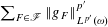 $\sum _{F\in \mathscr{F}}\Vert g_{F}\Vert _{L^{p^{\prime }}(\unicode[STIX]{x1D714})}^{p^{\prime }}$
. If
 $F\in \mathscr{F}$
, then
 $$\begin{eqnarray}\Vert g_{F}\Vert _{L^{p^{\prime }}(\unicode[STIX]{x1D714})}^{p^{\prime }}=\Vert 1_{E_{\mathscr{F}}(F)}g\Vert _{L^{p^{\prime }}(\unicode[STIX]{x1D714})}^{p^{\prime }}+\mathop{\sum }_{F^{\prime }\in \text{ch}_{\mathscr{ F}}^{\ast }(F)}(\langle g\rangle _{F^{\prime }}^{\unicode[STIX]{x1D714}})^{p^{\prime }}\unicode[STIX]{x1D714}(F^{\prime }).\end{eqnarray}$$
Clearly
 $$\begin{eqnarray}\mathop{\sum }_{F\in \mathscr{F}}\Vert 1_{E_{\mathscr{F}}(F)}g\Vert _{L^{p^{\prime }}(\unicode[STIX]{x1D714})}^{p^{\prime }}\leqslant \Vert g\Vert _{L^{p^{\prime }}(\unicode[STIX]{x1D714})}^{p^{\prime }},\end{eqnarray}$$
since the sets
 $E_{\mathscr{F}}(F),F\in \mathscr{F}$
, are pairwise disjoint. Rewriting the sum as in (3.5), the other term satisfies
 $$\begin{eqnarray}\displaystyle \mathop{\sum }_{F\in \mathscr{F}}\mathop{\sum }_{F^{\prime }\in \text{ch}_{\mathscr{ F}}^{\ast }(F)}(\langle g\rangle _{F^{\prime }}^{\unicode[STIX]{x1D714}})^{p^{\prime }}\unicode[STIX]{x1D714}(F^{\prime }) & {\leqslant} & \displaystyle 2^{p^{\prime }}\mathop{\sum }_{F\in \mathscr{F}}\mathop{\sum }_{\substack{ G\in \mathscr{G}: \\ \unicode[STIX]{x1D70B}_{\mathscr{F}}(G)=F\text{ or} \\ G\in \text{ch}_{\mathscr{F}}(F)}}(\langle g\rangle _{G}^{\unicode[STIX]{x1D714}})^{p^{\prime }}\mathop{\sum }_{\substack{ F^{\prime }\in \text{ch}_{\mathscr{ F}}(F) \\ \unicode[STIX]{x1D70B}_{\mathscr{G}}(F^{\prime })=G}}\unicode[STIX]{x1D714}(F^{\prime })\nonumber\\ \displaystyle & {\leqslant} & \displaystyle 2^{p^{\prime }}\mathop{\sum }_{F\in \mathscr{F}}\mathop{\sum }_{\substack{ G\in \mathscr{G}: \\ \unicode[STIX]{x1D70B}_{\mathscr{F}}(G)=F\text{ or} \\ G\in \text{ch}_{\mathscr{F}}(F)}}(\langle g\rangle _{G}^{\unicode[STIX]{x1D714}})^{p^{\prime }}\unicode[STIX]{x1D714}(G)\nonumber\\ \displaystyle & {\leqslant} & \displaystyle 2^{1+p^{\prime }}\mathop{\sum }_{G\in \mathscr{G}}(\langle g\rangle _{G}^{\unicode[STIX]{x1D714}})^{p^{\prime }}\unicode[STIX]{x1D714}(G)\lesssim \Vert g\Vert _{L^{p^{\prime }}(\unicode[STIX]{x1D714})}^{p^{\prime }}.\nonumber\end{eqnarray}$$
Thus, we have shown that
 $\sum _{F\in \mathscr{F}}\Vert g_{F}\Vert _{L^{p^{\prime }}(\unicode[STIX]{x1D714})}^{p^{\prime }}\lesssim \Vert g\Vert _{L^{p^{\prime }}(\unicode[STIX]{x1D714})}^{p^{\prime }},$
and this concludes the proof of Theorem 1.1.◻
Let us now discuss how one can arrive at the definition (1.6) of the test functions
 $\unicode[STIX]{x1D711}_{Q}$
. Suppose we want to find a family
 $\{\unicode[STIX]{x1D703}_{Q}\}_{Q\in \mathscr{D}}$
of non-negative
 $\unicode[STIX]{x1D70E}\times \unicode[STIX]{x1D702}$
-measurable functions such that if
 $$\begin{eqnarray}\unicode[STIX]{x1D6EC}_{Q}(\unicode[STIX]{x1D703}_{Q},g)\leqslant C_{1}\Vert \unicode[STIX]{x1D703}_{Q}\Vert _{L^{p}(\unicode[STIX]{x1D70E};\ell ^{2})}\Vert g\Vert _{L^{p^{\prime }}(\unicode[STIX]{x1D714})}\end{eqnarray}$$
and
 $$\begin{eqnarray}\unicode[STIX]{x1D6EC}_{Q}(f,1_{Q})\leqslant C_{2}\Vert f\Vert _{L^{p}(\unicode[STIX]{x1D70E};\ell ^{2})}\Vert 1_{Q}\Vert _{L^{p^{\prime }}(\unicode[STIX]{x1D714})}\end{eqnarray}$$
hold uniformly for
 $Q\in \mathscr{D}$
and non-negative functions
 $f$
and
 $g$
, then
 $$\begin{eqnarray}\unicode[STIX]{x1D6EC}(f,g)\lesssim (C_{1}+C_{2})\Vert f\Vert _{L^{p}(\unicode[STIX]{x1D70E};\ell ^{2})}\Vert g\Vert _{L^{p^{\prime }}(\unicode[STIX]{x1D714})}\end{eqnarray}$$
holds for all non-negative
 $f$
and
 $g$
. To find this kind of family, we first assume that
 $\{\unicode[STIX]{x1D703}_{Q}\}_{Q\in \mathscr{D}}$
is some collection of functions such that (3.9) and (3.10) hold, and then try to follow the method of parallel stopping cubes. We can proceed precisely as in §3 until we have to prove the estimate
 $$\begin{eqnarray}\mathop{\sum }_{F\in \mathscr{F}}\biggl(\frac{\iint _{\widehat{F}}f\unicode[STIX]{x1D707}\,\mathit{d}\unicode[STIX]{x1D702}\,\mathit{d}\unicode[STIX]{x1D70E}}{\iint _{\widehat{F}}\unicode[STIX]{x1D703}_{F}\unicode[STIX]{x1D707}\,\mathit{d}\unicode[STIX]{x1D702}\,\mathit{d}\unicode[STIX]{x1D70E}}\biggr)^{p}\Vert \unicode[STIX]{x1D703}_{F}\Vert _{L^{p}(\unicode[STIX]{x1D70E};\ell ^{2})}^{p}\lesssim \Vert f\Vert _{L^{p}(\unicode[STIX]{x1D70E};\ell ^{2})}^{p},\end{eqnarray}$$
where now the collection
 $\mathscr{F}$
is defined with the functions
 $\unicode[STIX]{x1D703}_{Q}$
instead of
 $\unicode[STIX]{x1D711}_{Q}$
.
To prove (3.11), we might want to minimize the ratios
 $$\begin{eqnarray}\frac{\Vert \unicode[STIX]{x1D703}_{F}\Vert _{L^{p}(\unicode[STIX]{x1D70E};\ell ^{2})}^{p}}{\left(\iint _{\widehat{F}}\unicode[STIX]{x1D703}_{F}\unicode[STIX]{x1D707}\,\mathit{d}\unicode[STIX]{x1D702}\,\mathit{d}\unicode[STIX]{x1D70E}\right)^{p}}.\end{eqnarray}$$
However, one should note that this is not directly a minimization of the sum in the left-hand side of (3.11), because the collection
 $\mathscr{F}$
depends on the choice of the functions
 $\unicode[STIX]{x1D703}_{Q}$
.
Hölder’s inequality implies
 $$\begin{eqnarray}\frac{\Vert \unicode[STIX]{x1D703}_{F}\Vert _{L^{p}(\unicode[STIX]{x1D70E};l^{2})}^{p}}{\left(\iint _{\widehat{F}}\unicode[STIX]{x1D703}_{F}\unicode[STIX]{x1D707}\,\mathit{d}\unicode[STIX]{x1D702}\,\mathit{d}\unicode[STIX]{x1D70E}\right)^{p}}\geqslant \frac{1}{\Vert 1_{\widehat{F}}\unicode[STIX]{x1D707}\Vert _{L^{p^{\prime }}(\unicode[STIX]{x1D70E};\ell ^{2})}^{p}},\end{eqnarray}$$
and equality is reached with
 $$\begin{eqnarray}\unicode[STIX]{x1D703}_{F}=|1_{\widehat{F}}\unicode[STIX]{x1D707}|_{\ell ^{2}}^{p^{\prime }-2}1_{\widehat{F}}\unicode[STIX]{x1D707}.\end{eqnarray}$$
This is the definition given in (1.6).
One may wonder what happens if one tries to find in this way a family
 $\{\unicode[STIX]{x1D717}_{Q}\}_{Q\in \mathscr{D}}$
of test functions in place of the indicators in (3.10). Then one would be led to minimize the ratios
 $$\begin{eqnarray}\frac{\Vert \unicode[STIX]{x1D717}_{G}\Vert _{L^{p^{\prime }}(\unicode[STIX]{x1D714})}^{p^{\prime }}}{\left(\int _{G}\unicode[STIX]{x1D717}_{G}\,\mathit{d}\unicode[STIX]{x1D714}\right)^{p^{\prime }}}\end{eqnarray}$$
for
 $G$
in some collection of dyadic cubes. Again by Hölder’s inequality this is minimized by
 $\unicode[STIX]{x1D717}_{G}=1_{G}$
.
4 Open problems and discussion
As mentioned in the Introduction, the problem of this paper arose when we tried to build two-weight
 $L^{p}$
-theory for the Hilbert transform. One part in the existing
 $L^{2}$
-theory is to bound the so-called tail form. In [Reference Hytönen2, §6], this part is reduced to an estimate of the form
 $$\begin{eqnarray}(f,g)\mapsto \mathop{\sum }_{Q\in \mathscr{D}}\unicode[STIX]{x1D706}_{Q}\int _{Q_{+}}f\,\mathit{d}\unicode[STIX]{x1D70E}\int _{Q_{-}}g\,\mathit{d}\unicode[STIX]{x1D714}\lesssim \Vert f\Vert _{L^{2}(\unicode[STIX]{x1D70E})}\Vert g\Vert _{L^{2}(\unicode[STIX]{x1D714})},\end{eqnarray}$$
where
 $Q_{+}$
and
 $Q_{-}$
are two distinguished child cubes of the cube
 $Q\in \mathscr{D}$
. The estimate
 $$\begin{eqnarray}\mathop{\sum }_{Q\in \mathscr{D}}\unicode[STIX]{x1D706}_{Q}\iint _{\widehat{Q}}f\unicode[STIX]{x1D707}\,\mathit{d}\unicode[STIX]{x1D702}\,\mathit{d}\unicode[STIX]{x1D70E}\int _{Q}g\,\mathit{d}\unicode[STIX]{x1D714}\lesssim \Vert f\Vert _{L^{p}(\unicode[STIX]{x1D70E};\ell ^{2})}\Vert g\Vert _{L^{p^{\prime }}(\unicode[STIX]{x1D714})}\end{eqnarray}$$
came up as a model problem when we considered possible
 $L^{p}$
-generalizations related to the tail form.
We raise here the following question: If
 $p\in (1,2)$
, when does estimate (4.1) hold? In order to suggest one approach, we briefly describe some results related to the operator
 $S^{\unicode[STIX]{x1D70E}}f:=\sum _{Q\in \mathscr{D}}\unicode[STIX]{x1D706}_{Q}\int _{Q}f\,\mathit{d}\unicode[STIX]{x1D70E}1_{Q}.$
Let
 $S^{\unicode[STIX]{x1D714}}$
be the corresponding operator with the measure
 $\unicode[STIX]{x1D714}$
.
The
 $L^{2}$
-result from [Reference Nazarov, Treil and Volberg8] and its generalization in [Reference Lacey, Sawyer and Uriarte-Tuero6], mentioned in the Introduction, state that if
 $1<p\leqslant q<\infty$
, then a similar theorem as Theorem 1.1 characterizes boundedness of
 $S^{\unicode[STIX]{x1D70E}}$
from
 $L^{p}(\unicode[STIX]{x1D70E})$
into
 $L^{q}(\unicode[STIX]{x1D714})$
;
 $S^{\unicode[STIX]{x1D70E}}$
is bounded if and only if
 $S^{\unicode[STIX]{x1D70E}}$
and
 $S^{\unicode[STIX]{x1D714}}$
satisfy a testing condition with indicators
 $1_{Q}$
of dyadic cubes
 $Q\in \mathscr{D}$
. Boundedness of
 $S^{\unicode[STIX]{x1D70E}}:L^{p}(\unicode[STIX]{x1D70E})\rightarrow L^{q}(\unicode[STIX]{x1D714})$
in the range
 $1<q<p<\infty$
was characterized by Tanaka [Reference Tanaka10] in terms of a discrete Wolff’s potential. See also a unified theorem for all exponents
 $p,q\in (1,\infty )$
by Hänninen, Hytönen and Li [Reference Hänninen, Hytönen and Li.1]. In [Reference Hänninen, Hytönen and Li.1] it was shown that the indicator testing conditions do not imply boundedness of
 $S^{\unicode[STIX]{x1D70E}}:L^{p}(\unicode[STIX]{x1D70E})\rightarrow L^{q}(\unicode[STIX]{x1D714})$
if
 $1<q<p<\infty$
; this example is even in the case when both the measures
 $\unicode[STIX]{x1D70E}$
and
 $\unicode[STIX]{x1D714}$
are equal to the Lebesgue measure.
The estimate (4.1) can be equivalently formulated as the boundedness of
 $$\begin{eqnarray}T^{\unicode[STIX]{x1D70E}}f:=\mathop{\sum }_{Q\in \mathscr{D}}\unicode[STIX]{x1D706}_{Q}\iint _{\widehat{Q}}f\unicode[STIX]{x1D707}\,\mathit{d}\unicode[STIX]{x1D702}\,\mathit{d}\unicode[STIX]{x1D70E}1_{Q}\end{eqnarray}$$
from
 $L^{p}(\unicode[STIX]{x1D70E};\ell ^{2})$
into
 $L^{p}(\unicode[STIX]{x1D714})$
. The fact that we were not able to characterize the estimate (4.1) when
 $p\in (1,2)$
somewhat fits to the known results about boundedness of
 $S^{\unicode[STIX]{x1D70E}}:L^{p}(\unicode[STIX]{x1D70E})\rightarrow L^{q}(\unicode[STIX]{x1D714})$
and the relative order of the exponents
 $p$
and
 $q$
. Namely, with the operator
 $S^{\unicode[STIX]{x1D70E}}$
the indicator testing conditions imply boundedness only when
 $1<p\leqslant q<\infty$
and in the range
 $p\geqslant 2$
where we can characterize boundedness of
 $T^{\unicode[STIX]{x1D70E}}$
, the exponent
 $p$
related to
 $L^{p}(\unicode[STIX]{x1D714})$
is greater than or equal to both the exponents
 $2$
and
 $p$
related to
 $L^{p}(\unicode[STIX]{x1D70E};\ell ^{2})$
.
The approach to studying boundedness of
 $T^{\unicode[STIX]{x1D70E}}:L^{p}(\unicode[STIX]{x1D70E};\ell ^{2})\rightarrow L^{p}(\unicode[STIX]{x1D714})$
,
 $p\in (1,2)$
, that we propose here, is to use a certain quadratic testing that was introduced by the second author in [Reference Vuorinen11, Reference Vuorinen12] and was introduced to the second author by the first author in connection with a PhD project. It was shown in [Reference Vuorinen11] that if
 $p,q\in (1,\infty )$
, then
 $S^{\unicode[STIX]{x1D70E}}:L^{p}(\unicode[STIX]{x1D70E})\rightarrow L^{q}(\unicode[STIX]{x1D714})$
is bounded if and only if
 $S^{\unicode[STIX]{x1D70E}}$
and
 $S^{\unicode[STIX]{x1D714}}$
satisfy the quadratic testing condition.
Suppose
 $p\in (1,\infty )$
. Define again the test functions
 $$\begin{eqnarray}\unicode[STIX]{x1D711}_{Q}:=|1_{\widehat{Q}}\unicode[STIX]{x1D707}|_{\ell ^{2}}^{p^{\prime }-2}1_{\widehat{Q}}\unicode[STIX]{x1D707},\quad Q\in \mathscr{D}.\end{eqnarray}$$
For
 $Q\in \mathscr{D}$
let
 $T_{Q}^{\unicode[STIX]{x1D70E}}$
be the corresponding localized version of the operator, defined with the sum extending only over
 $Q^{\prime }\subset Q$
. Let
 $\mathscr{T}_{p}^{\unicode[STIX]{x1D70E}}$
be the smallest possible constant such that
 $$\begin{eqnarray}\biggl\|\biggl(\mathop{\sum }_{Q\in \mathscr{D}}(a_{Q}T_{Q}^{\unicode[STIX]{x1D70E}}\unicode[STIX]{x1D711}_{Q})^{2}\biggr)^{1/2}\biggr\|_{L^{p}(\unicode[STIX]{x1D714})}\leqslant \mathscr{T}_{p}^{\unicode[STIX]{x1D70E}}\biggl\|\biggl(\mathop{\sum }_{Q\in \mathscr{D}}(a_{Q}\unicode[STIX]{x1D711}_{Q})^{2}\biggr)^{1/2}\biggr\|_{L^{p}(\unicode[STIX]{x1D70E};\ell ^{2})}\end{eqnarray}$$
holds for all collections
 $\{a_{Q}\}_{Q\in \mathscr{D}}$
of real numbers, with the understanding that
 $\mathscr{T}_{p}^{\unicode[STIX]{x1D70E}}$
may be
 $\infty$
. We say that
 $T^{\unicode[STIX]{x1D70E}}$
satisfies the quadratic testing condition in
 $L^{p}$
if the constant
 $\mathscr{T}_{p}^{\unicode[STIX]{x1D70E}}$
is finite. Similarly, we define the quadratic testing constant
 $\mathscr{T}_{p^{\prime }}^{\unicode[STIX]{x1D714}}$
for the formal adjoint operator
 $T^{\unicode[STIX]{x1D714}}g:=\sum _{Q\in \mathscr{D}}\unicode[STIX]{x1D706}_{Q}\int _{Q}g\,\mathit{d}\unicode[STIX]{x1D714}1_{\widehat{Q}}\unicode[STIX]{x1D707}$
using indicators
 $1_{Q},Q\in \mathscr{D},$
as test functions.
The precise question we want to ask is as follows.
Question 4.1. Let
 $p\in (1,2)$
. If
 $\mathscr{T}_{p}^{\unicode[STIX]{x1D70E}}+\mathscr{T}_{p^{\prime }}^{\unicode[STIX]{x1D714}}<\infty$
, then does it follow that
 $T^{\unicode[STIX]{x1D70E}}:L^{p}(\unicode[STIX]{x1D70E};\ell ^{2})\rightarrow L^{p}(\unicode[STIX]{x1D714})$
is bounded and that the estimate
 $$\begin{eqnarray}\Vert T^{\unicode[STIX]{x1D70E}}f\Vert _{L^{p}(\unicode[STIX]{x1D714})}\lesssim (\mathscr{T}_{p}^{\unicode[STIX]{x1D70E}}+\mathscr{T}_{p^{\prime }}^{\unicode[STIX]{x1D714}})\Vert f\Vert _{L^{p}(\unicode[STIX]{x1D70E};\ell ^{2})},\quad f\in L^{p}(\unicode[STIX]{x1D70E};\ell ^{2}),\end{eqnarray}$$
holds?
We remark that when
 $p\in (1,2)$
it is possible that one should use some other class of test functions than the ones defined in (4.2); when using quadratic testing the proof does not offer a similar situation as described in the end of §3 to guess the test functions.
It is not immediately obvious that the quadratic testing condition is a necessary consequence of boundedness of
 $T^{\unicode[STIX]{x1D70E}}$
; nevertheless it follows in the spirit of a classical theorem by Marcinkiewicz and Zygmund [Reference Marcinkiewicz and Zygmund7] that if
 $T^{\unicode[STIX]{x1D70E}}:L^{p}(\unicode[STIX]{x1D70E};\ell ^{2})\rightarrow L^{p}(\unicode[STIX]{x1D714})$
is bounded, then
 $\mathscr{T}_{p}^{\unicode[STIX]{x1D70E}}+\mathscr{T}_{p^{\prime }}^{\unicode[STIX]{x1D714}}\lesssim \Vert T^{\unicode[STIX]{x1D70E}}\Vert _{L^{p}(\unicode[STIX]{x1D70E};\ell ^{2})\rightarrow L^{p}(\unicode[STIX]{x1D714})}$
, see [Reference Vuorinen11] or [Reference Vuorinen12].
Two-weight inequality of the Hilbert transform
Finally, we state our conjecture about the two-weight inequality of the Hilbert transform in
 $L^{p}$
. In the following we assume that
 $\unicode[STIX]{x1D70E}$
and
 $\unicode[STIX]{x1D714}$
are non-negative locally finite Borel measures in
 $\mathbb{R}$
. We shall somewhat imprecisely just talk about the Hilbert transform as an operator
 $H^{\unicode[STIX]{x1D70E}}$
or
 $H^{\unicode[STIX]{x1D714}}$
, where
 $\unicode[STIX]{x1D70E}$
and
 $\unicode[STIX]{x1D714}$
refer to the measure of integration in the definition of these operators. The operators
 $H^{\unicode[STIX]{x1D70E}}$
and
 $H^{\unicode[STIX]{x1D714}}$
should be thought of as formal adjoints of each other, in the sense that
 $$\begin{eqnarray}\int _{\mathbb{R}}gH^{\unicode[STIX]{x1D70E}}(f)\,\mathit{d}\unicode[STIX]{x1D714}=-\int _{\mathbb{R}}fH^{\unicode[STIX]{x1D714}}(g)\,\mathit{d}\unicode[STIX]{x1D70E}=\iint _{\mathbb{R}\times \mathbb{R}}\frac{g(x)f(y)}{x-y}\,\mathit{d}\unicode[STIX]{x1D714}(x)\,\mathit{d}\unicode[STIX]{x1D70E}(y)\end{eqnarray}$$
for
 $f$
and
 $g$
in a suitable class of functions. We refer to [Reference Lacey4, Reference Lacey, Sawyer, Shen and Uriarte-Tuero5] and [Reference Hytönen2] for a precise definition of the Hilbert transform in this two-weight setting.
Let
 $p\in (1,\infty )$
. We say that
 $H^{\unicode[STIX]{x1D70E}}$
satisfies the global quadratic testing condition in
 $L^{p}$
if there exists a constant
 $C$
such that the inequality
 $$\begin{eqnarray}\mathop{\biggl\|\biggl(\mathop{\sum }_{i=1}^{\infty }(a_{i}H^{\unicode[STIX]{x1D70E}}1_{I_{i}})^{2}\biggr)^{1/2}\biggr\|}\nolimits_{L^{p}(\unicode[STIX]{x1D714})}\leqslant C\mathop{\biggl\|\biggl(\mathop{\sum }_{i=1}^{\infty }(a_{i}1_{I_{i}})^{2}\biggr)^{1/2}\biggr\|}\nolimits_{L^{p}(\unicode[STIX]{x1D70E})}\end{eqnarray}$$
holds for all collections
 $\{I_{i}\}_{i=1}^{\infty }$
of intervals in
 $\mathbb{R}$
and all collections
 $\{a_{i}\}_{i=1}^{\infty }$
of real numbers. The smallest possible constant
 $\mathscr{H}_{p}^{\unicode[STIX]{x1D70E}}$
in this inequality is the quadratic testing constant for
 $H^{\unicode[STIX]{x1D70E}}$
. Similarly, we define the testing constant
 $\mathscr{H}_{p^{\prime }}^{\unicode[STIX]{x1D714}}$
for the operator
 $H^{\unicode[STIX]{x1D714}}$
by replacing
 $H^{\unicode[STIX]{x1D70E}}$
with
 $H^{\unicode[STIX]{x1D714}}$
,
 $p$
with
 $p^{\prime }$
and reversing the roles of
 $\unicode[STIX]{x1D70E}$
and
 $\unicode[STIX]{x1D714}$
in (4.4).
In [Reference Lacey4, Reference Lacey, Sawyer, Shen and Uriarte-Tuero5] and [Reference Hytönen2] it was shown that the two-weight inequality
 $$\begin{eqnarray}\Vert H^{\unicode[STIX]{x1D70E}}f\Vert _{L^{2}(\unicode[STIX]{x1D714})}\leqslant C\Vert f\Vert _{L^{2}(\unicode[STIX]{x1D70E})},\quad f\in L^{2}(\unicode[STIX]{x1D70E}),\end{eqnarray}$$
holds if and only if
 $H^{\unicode[STIX]{x1D70E}}$
and
 $H^{\unicode[STIX]{x1D714}}$
satisfy a global indicator testing condition if and only if
 $H^{\unicode[STIX]{x1D70E}}$
and
 $H^{\unicode[STIX]{x1D714}}$
satisfy a local indicator testing condition and Muckenhoupt–Poisson two-weight
 $A_{2}$
condition holds. Moreover, the smallest constant
 $\mathscr{N}_{2}$
in (4.5) satisfies
 $$\begin{eqnarray}\mathscr{N}_{2}\simeq \mathscr{H}_{2}^{\unicode[STIX]{x1D70E}}+\mathscr{H}_{2}^{\unicode[STIX]{x1D714}},\end{eqnarray}$$
and there is also an equivalence with suitable local testing constants and a two-weight
 $A_{2}$
constant; see the cited papers for details. We remark that in
 $L^{2}$
the quadratic testing conditions are equivalent with the indicator testing conditions; hence we use the same notation for the constants.
Conjecture 4.2. Let
 $p\in (1,\infty )$
. There exists a constant
 $C$
such that the Hilbert transform
 $H^{\unicode[STIX]{x1D70E}}$
satisfies the two-weight inequality
 $$\begin{eqnarray}\Vert H^{\unicode[STIX]{x1D70E}}f\Vert _{L^{p}(\unicode[STIX]{x1D714})}\leqslant C\Vert f\Vert _{L^{p}(\unicode[STIX]{x1D70E})},\quad f\in L^{p}(\unicode[STIX]{x1D70E}),\end{eqnarray}$$
if and only if
 $H^{\unicode[STIX]{x1D70E}}$
and
 $H^{\unicode[STIX]{x1D714}}$
satisfy the global quadratic testing conditions in
 $L^{p}$
and
 $L^{p^{\prime }}$
, respectively. Moreover, the smallest possible constant
 $\mathscr{N}_{p}$
in (4.6) satisfies
 $$\begin{eqnarray}\mathscr{N}_{p}\simeq _{p}\mathscr{H}_{p}^{\unicode[STIX]{x1D70E}}+\mathscr{H}_{p^{\prime }}^{\unicode[STIX]{x1D714}}.\end{eqnarray}$$
We also think that the two-weight inequality can be characterized in terms of certain local testing conditions together with a condition on the measures. Let
 $p\in (1,\infty )$
. We say that
 $H^{\unicode[STIX]{x1D70E}}$
satisfies the local quadratic testing condition if for some constant
 $C$
 $$\begin{eqnarray}\mathop{\biggl\|\biggl(\mathop{\sum }_{i=1}^{\infty }\big(a_{i}1_{I_{i}}H^{\unicode[STIX]{x1D70E}}1_{I_{i}}\big)^{2}\biggr)^{1/2}\biggr\|}\nolimits_{L^{p}(\unicode[STIX]{x1D714})}\leqslant C\mathop{\biggl\|\biggl(\mathop{\sum }_{i=1}^{\infty }(a_{i}1_{I_{i}})^{2}\biggr)^{1/2}\biggr\|}\nolimits_{L^{p}(\unicode[STIX]{x1D70E})}\end{eqnarray}$$
holds for all collections
 $\{I_{i}\}_{i=1}^{\infty }$
of intervals in
 $\mathbb{R}$
and all collections
 $\{a_{i}\}_{i=1}^{\infty }$
of real numbers. The dual condition for
 $H^{\unicode[STIX]{x1D714}}$
is obtained from (4.7) by replacing
 $p$
by
 $p^{\prime }$
and reversing the roles of the measures. We denote the smallest possible constants by
 $\mathscr{H}_{p,\text{loc}}^{\unicode[STIX]{x1D70E}}$
and
 $\mathscr{H}_{p^{\prime },\text{loc}}^{\unicode[STIX]{x1D714}}$
.
If there exists a constant
 $C$
such that
 $$\begin{eqnarray}\mathop{\biggl\|\biggl(\mathop{\sum }_{i=1}^{\infty }(1_{I_{i}}\int _{I_{i}^{c}}\frac{|f_{i}(x)|}{|x-c_{i}|}\,\mathit{d}\unicode[STIX]{x1D70E}(x))^{2}\biggr)^{1/2}\biggr\|}\nolimits_{L^{p}(\unicode[STIX]{x1D714})}\leqslant C\mathop{\biggl\|\biggl(\mathop{\sum }_{i=1}^{\infty }|f_{i}|^{2}\biggr)^{1/2}\biggr\|}\nolimits_{L^{p}(\unicode[STIX]{x1D70E})}\end{eqnarray}$$
holds for all collections
 $\{I_{i}\}_{i=1}^{\infty }$
of intervals and all collections
 $\{f_{i}\}_{i=1}^{\infty }$
of functions, we say that the pair
 $(\unicode[STIX]{x1D70E},\unicode[STIX]{x1D714})$
of measures satisfies a (one-sided) quadratic Muckenhoupt–Poisson two-weight
 $A_{p}$
condition. Here
 $I^{c}$
is the complement of the interval
 $I$
. We denote the smallest constant
 $C$
in (4.8) by
 $[\unicode[STIX]{x1D70E},\unicode[STIX]{x1D714}]_{p}$
. We will also need the dual condition of (4.8), which is obtained from (4.8) by replacing
 $p$
by
 $p^{\prime }$
and reversing the roles of the measures. The best constant in the dual inequality is denoted by
 $[\unicode[STIX]{x1D714},\unicode[STIX]{x1D70E}]_{p^{\prime }}$
. We note that these conditions are positive in the sense that there is no cancellation involved.
We still formulate one condition, which we define to be satisfied if and only if there exists a constant
 $C$
such that
 $$\begin{eqnarray}\displaystyle & & \displaystyle \mathop{\sum }_{i=1}^{\infty }|\langle a_{i}H^{\unicode[STIX]{x1D70E}}1_{I_{i}},b_{i}1_{J(I_{i})}\rangle _{\unicode[STIX]{x1D714}}|\nonumber\\ \displaystyle & & \displaystyle \quad \leqslant C\mathop{\biggl\|\biggl(\mathop{\sum }_{i=1}^{\infty }|a_{i}1_{I_{i}}|^{2}\biggr)^{1/2}\biggr\|}\nolimits_{L^{p}(\unicode[STIX]{x1D70E})}\mathop{\biggl\|\biggl(\mathop{\sum }_{i=1}^{\infty }|b_{i}1_{J(I_{i})}|^{2}\biggr)^{1/2}\biggr\|}\nolimits_{L^{p^{\prime }}(\unicode[STIX]{x1D714})}\end{eqnarray}$$
holds for all collections
 $\{I_{i}\}_{i=1}^{\infty }$
of intervals and all collections
 $\{a_{i}\}_{i=1}^{\infty }$
,
 $\{b_{i}\}_{i=1}^{\infty }$
of real numbers. Here
 $J(I_{i})$
is an interval of equal length with
 $I_{i}$
and adjacent to
 $I_{i}$
. If (4.9) is satisfied, let us denote the smallest constant
 $C$
in the inequality by
 $\mathscr{T}$
.
In addition to Conjecture 4.2 we suspect that the two-weight inequality (4.6) holds if and only if the local quadratic testing conditions, the quadratic Muckenhoupt–Poisson two-weight
 $A_{p}$
condition and the condition (4.9) hold and that we have the estimate
 $$\begin{eqnarray}\mathscr{N}_{p}\simeq _{p}\mathscr{H}_{p,\text{loc}}^{\unicode[STIX]{x1D70E}}+\mathscr{H}_{p^{\prime },\text{loc}}^{\unicode[STIX]{x1D714}}+[\unicode[STIX]{x1D70E},\unicode[STIX]{x1D714}]_{p}+[\unicode[STIX]{x1D714},\unicode[STIX]{x1D70E}]_{p^{\prime }}+\mathscr{T}.\end{eqnarray}$$
At the moment it is unclear whether (4.9) follows from (4.7), (4.8) and their dual statements. In any case, all the conditions are necessary for the two-weight inequality and the estimate “
 ${\gtrsim}_{p}$
” in (4.10) holds. The known
 $L^{2}$
-result is analogous to (4.10), except that in the
 $L^{2}$
-case the condition (4.9) is known to follow from the Muckenhoupt–Poisson
 $A_{2}$
condition.
Acknowledgements
Both authors were supported by the ERC Starting Grant “Analytic–probabilistic methods for borderline singular integrals”. They are members of the Finnish Centre of Excellence in Analysis and Dynamics Research.


