



1. Introduction
Laminar-to-turbulence transition has been a long-lasting challenge for the fluid mechanics community due to its high sensitivity to environmental uncertainties. Even a small change in the spectral makeup of the free-stream conditions can lead to qualitative changes in the transition mechanism and quantitative changes in its location. Measurements, or observations, can help reduce these uncertainties (Zaki Reference Zaki2025); however, in realistic configurations, flow data are often only available at the wall. In this work, we attempt to predict the inflow conditions that result in the available wall measurements under the scenario of bypass transition. The results demonstrate how the chaotic nature of transition complicates this task and serve as a benchmark for other algorithms addressing this challenge.
The boundary-layer flow is known to amplify environmental disturbances, generating large coherent structures whose breakdown leads to transition to turbulence. When this process involves discrete instability waves at supercritical Reynolds numbers, it is termed orderly or natural transition. However, in the presence of finite-amplitude environmental perturbations, especially broadband free-stream turbulence (FST), another form of transition process, termed bypass transition, takes place (Zaki Reference Zaki2013). The boundary layer filters the free-stream spectrum and only low-frequency disturbances are amplified by the mean shear. These disturbances subsequently undergo secondary instabilities, which give way to sporadic bursts of turbulent spots. The spots, which spread as they advect downstream, already exhibit a fully turbulent dynamics within their core (Nolan & Zaki Reference Nolan and Zaki2013; Marxen & Zaki Reference Marxen and Zaki2019) and a fractal geometry at the interface that separates them from the outside laminar flow (Wu et al. Reference Wu, Zaki and Meneveau2020). Bypass transition is therefore chaotic in its onset and evolution, and its detailed description is sensitive to the environmental conditions, making it inherently challenging to compute flow sensitivity for applications like optimal control, optimal perturbation analyses and estimation of flow conditions.
Techniques for estimating instantaneous flow states or predicting the evolution of flow variables can be generally classified as data driven and model based. The data-driven method seeks the relationship between the measurements, i.e. input, and the flow state, i.e. output, without any prior knowledge of the mathematical equations governing the flow. Linear stochastic estimation, which utilises second-order correlations between the measured data and the variable to be predicted, is one of the data-driven techniques and has been used to estimate wall-bounded turbulent flow (Adrian & Moin Reference Adrian and Moin1988; Suzuki & Hasegawa Reference Suzuki and Hasegawa2017; Liu & Hasegawa Reference Liu and Hasegawa2020). Additionally, owing to the rapid development of computer hardware and numerical algorithms in the past decade, artificial neural networks (ANNs) have demonstrated growing success in predicting turbulence (Milano & Koumoutsakos Reference Milano and Koumoutsakos2002; Fukami et al. Reference Fukami, Fukagata and Taira2019; Du et al. Reference Du, Wang and Zaki2023). By learning complex patterns and features from large datasets, ANN models can capture the intricate dynamics of turbulent flows that traditional methods may miss (Duraisamy et al. Reference Duraisamy, Iaccarino and Xiao2019).
In contrast to data-driven approaches, which usually require massive data, the model-based method is built on the governing equations that describe flow systems. Among these approaches, resolvent-based estimation has emerged as a promising framework for reconstructing unmeasured flow quantities from limited observations. Building on the resolvent framework of McKeon & Sharma (Reference McKeon and Sharma2010), in which the Navier–Stokes equations linearised around the mean are driven by the nonlinear terms considered as a forcing, Towne et al. (Reference Towne, Lozano-Duran and Yang2020) introduced a statistical resolvent-based method that infers the cross-spectral density of the nonlinear forcing from limited data and, via the resolvent operator, estimates the corresponding space–time flow statistics without a rank-1 assumption. Subsequently, Martini et al. (Reference Martini, Jordan, Cavalieri, Towne and Lesshafft2020) extended the approach to an optimal estimator for time-varying flow fields in transitional and turbulent regimes. Their method, based on a matrix-free implementation of direct and adjoint linearised operators, enables accurate estimation without relying on a priori model reduction. More recently, Amaral et al. (Reference Amaral, Cavalieri, Martini, Jordan and Towne2021) applied the resolvent-based method to turbulent channel flow and showed that structures leaving measurable footprints can be accurately estimated from wall shear stress and pressure data across a wide Reynolds number range.
A key advantage of resolvent-based approaches lies in their incorporation of prior physical knowledge through linearised operators, which act as a regularising mechanism and enhance estimation robustness, particularly under sparse observational conditions. In contrast, other model-based estimation methods, such as those extensively developed and widely applied in the meteorological community, primarily rely on observational data to constrain model evolution (Rabier Reference Rabier2005; Kalnay et al. Reference Kalnay, Li, Miyoshi, Yang and Ballabrera-Poy2007). These approaches are typically Bayesian-based and include traditional variation data assimilation (Talagrand & Courtier Reference Talagrand and Courtier1987; Rawlins et al. Reference Rawlins, Ballard, Bovis, Clayton, Li, Inverarity, Lorenc and Payne2007), ensemble-based Kalman filters (Houtekamer & Zhang Reference Houtekamer and Zhang2016) and Monte Carlo techniques. While the variational and ensemble methods are widely used in numerical weather prediction, each possesses inherent limitations (Bannister Reference Bannister2017), which has motivated the development of hybrid techniques that seek to combine their respective strengths while mitigating individual shortcomings (Zhang et al. Reference Zhang, Zhang and Hansen2009).
Inspired by similar principles, model-based estimation in fluid mechanics can also be categorised according to how measurements are assimilated: filtering methods update the flow state sequentially using the most recent data, whereas smoothing methods seek a state trajectory that best fits observations over an entire time window (Wang & Zaki Reference Wang and Zaki2021). Hœpffner et al. (Reference Hœpffner, Chevalier, Bewley and Henningson2005) used the Kalman filter, a typical filter approach, to estimate perturbations in laminar flows. To account for nonlinearity, Chevalier et al. (Reference Chevalier, Hœpffner, Bewley and Henningson2006) and Colburn et al. (Reference Colburn, Cessna and Bewley2011) applied the extended Kalman filter and ensemble Kalman filter, respectively, to estimate turbulent channel flow from wall measurements. However, as mentioned before, since the filtering approach attempts to match the measurement at the last moment rather than over the entire interval, its accuracy is limited (Zaki & Wang Reference Zaki and Wang2021).
In contrast, the smoothing approaches seek to estimate the entire flow state over a finite time window, such that the predicted evolution of the nonlinear system optimally matches the available measurements throughout the interval (Bewley & Protas Reference Bewley and Protas2004). It typically uses iterative looping over the forward and adjoint equations, where the optimal initial conditions, boundary conditions or model parameters are obtained by defining a cost function that measures the differences between the estimation and target data. Adjoint techniques have shown success in finding optimal boundary conditions in transitional flow (Mao et al. Reference Mao, Blackburn and Sherwin2013, Reference Mao, Zaki, Sherwin and Blackburn2017), suppressing transitional flow (Xiao & Papadakis Reference Xiao and Papadakis2017) and estimating scalar sources from remote measurements in turbulent flow (Wang et al. Reference Wang, Hasegawa and Zaki2019b ). More recently, Wang & Zaki (Reference Wang and Zaki2021) applied an adjoint-variational approach to estimate the initial condition of turbulent channel flow from limited measurements of velocity data.
While many of the aforementioned estimation strategies have demonstrated success in channel flows, their extension to boundary-layer flows has been less explored. Here, we consider a spatially developing transitional boundary layer and perform wall-based estimation using an adjoint-variational framework. As noted by Bewley et al. (Reference Bewley, Moin and Temam2001), one of the earliest applications of adjoint-based optimisation to turbulent flows, the framework is computationally intensive and therefore currently restricted to offline implementation; nevertheless, it provides an optimal benchmark, i.e. the best achievable performance permitted by the governing dynamics and the available observations. The present study aims to explore the theoretical limits of reconstructing boundary-layer flows from an observer’s perspective and to quantify flow observability (Zaki Reference Zaki2025).
The rest of the paper is organised as follows. In
 $\S$
2, the adjoint-variational method, formulation of the Hessian matrix and the computational set-up are introduced. The proposed methods are first examined through the prediction of streaks induced by simple steady inflow with various turbulence intensities in
 $\S$
3. In
 $\S$
4, a more complex inflow profile with multiple vortical modes is constructed to demonstrate the prediction of streak meandering motions. Finally in
 $\S$
5, the prediction of bypass transition triggered by full-spectrum FST is performed with discussions on the performance, sensitivity to inflow conditions, effect of optimisation time and Hessian analysis. In
 $\S$
6 the main observations are summarised.
2. Theoretical formulation and computational set-up
2.1. Governing equations
The flow configuration of interest is a boundary layer developing over a flat plate with a slender elliptic leading edge, as shown in figure 1, which has been adopted in several previous studies (Mao et al. Reference Mao, Blackburn and Sherwin2013, Reference Mao, Blackburn and Sherwin2015; Wang et al. Reference Wang, Mao and Zaki2019a
). The leading edge is located at the origin and has an aspect ratio of
 $AR=20$
. The flow is governed by the incompressible Navier–Stokes (NS) equations,
 \begin{equation} \partial _t {\boldsymbol{u}}+ {\boldsymbol{u}} \boldsymbol{\cdot } \boldsymbol{\nabla }{\boldsymbol{u}} + \boldsymbol{\nabla }p - {\textit{Re}}^{-1} \boldsymbol{\nabla} ^2 {\boldsymbol{u}} =0, \ \ \ \boldsymbol{\nabla }\boldsymbol{\cdot }{\boldsymbol{u}} = 0, \end{equation}
where
 ${\boldsymbol{u}}= (u, v, w )^{\textrm {T}}$
and
 $p$
represent the non-dimensional velocity and pressure with
 $u$
,
 $v$
and
 $w$
being the streamwise, wall-normal and spanwise velocity components, respectively. The Reynolds number
 $Re=U_{\infty }R/\nu$
is based on the free-stream velocity
 $U_{\infty }$
, the kinematic viscosity
 $\nu$
and a reference length
 $R$
, which is the half-thickness of the flat plate. For analyses, the flow variables in (2.1) are decomposed as
 \begin{equation} \left ({\boldsymbol{u},p}\right ) = \left ({\boldsymbol{U},P}\right ) + \left ({\boldsymbol{u}}^{\prime },p^{\prime }\right ), \end{equation}
where
 $({\boldsymbol{U}},P)$
with
 ${\boldsymbol{U}}=(U,V, 0)^{\textrm {T}}$
is the two-dimensional (2-D) and steady solution of (2.1) and
 $({\boldsymbol{u}}^{\prime },p^{\prime })$
with
 ${\boldsymbol{u}}^{\prime }=(u^{\prime },v^{\prime },w^{\prime })^{\textrm {T}}$
is the perturbation. As bypass transition is convective and is triggered by the inflow disturbance, consider a flow starting from a 2-D steady solution of (2.1) and perturbed by an inflow condition in the form
 \begin{equation} {\boldsymbol{u}}({\boldsymbol{x}}_{\textit{in}},t) = U_{\infty }+G(t){\boldsymbol{u}}_{\textit{in}}, \end{equation}
where
 ${\boldsymbol{x}}_{\textit{in}}$
denotes the spatial coordinates on the inflow boundary. The parameter
 $G(t)$
is given by
 \begin{equation} G(t) = \big(1 - e ^ {-\sigma t^2}\big)\big(1 - e ^ {-\sigma (T - t)^2} \big), \end{equation}
where
 $\sigma$
is a relaxation factor and is set to
 $\sigma =100$
throughout this work and
 $T$
is the total optimisation time. Here,
 $G(t)$
is used to force the inflow
 ${\boldsymbol{u}}_{\textit{in}}$
at
 $t=0$
and
 $t=T$
to be zero, which eliminates spatial and temporal discontinuities that would otherwise arise during the forward and adjoint simulations. This formulation has been elaborated in Mao et al. (Reference Mao, Blackburn and Sherwin2013) and applied in several other scenarios (Mao et al. Reference Mao, Blackburn and Sherwin2015; Wang et al. Reference Wang, Mao and Zaki2019a
).
Schematic diagram of the flow configuration and the coordinate system. The leading edge is located at the origin.

2.2. Adjoint-variational optimisation
Owing to the convective nature of the flow scenario considered, the prediction of bypass transition can be realised through the prediction of the inflow profile, which leads to the same flow development as the reference one. The prediction is then transformed into an adjoint-based optimisation problem with an objective function defined based on the streamwise velocity gradient at the wall
 \begin{equation} J = \int _0^T \int _{S_W} \left ( \frac {\partial u}{\partial y} - \frac {\partial u_r}{\partial y} \right )^2 \textrm {d}S_W \textrm {d}t, \end{equation}
where
 $S_W$
denotes the part of the wall where data measurement is collected and the subscript
 $r$
denotes the reference variable. The streamwise velocity gradient is used in the objective function because pre-transitional flows are predominantly characterised by streamwise velocity fluctuations caused by the presence of velocity streaks (Matsubara & Alfredsson Reference Matsubara and Alfredsson2001).
A Lagrangian
 $\mathcal{L}$
is defined with the aim of obtaining the inflow perturbation
 ${\boldsymbol{u}}^{\prime }_{\textit{in}} ({\boldsymbol{x}}_{\textit {\textit{in}}}, t )$
that minimises the objective function (2.5), while satisfying the governing (2.1)
 \begin{equation} \mathcal{L} = J - \int _0^T \int _{\varOmega } \left [ {\boldsymbol{u}}^{\dagger } \boldsymbol{\cdot }\left ( \partial _t {\boldsymbol{u}}+ {\boldsymbol{u}} \boldsymbol{\cdot }\boldsymbol{\nabla }{\boldsymbol{u}} + \boldsymbol{\nabla }p - {\textit{Re}}^{-1} \boldsymbol{\nabla} ^2 {\boldsymbol{u}} \right ) + p^{\dagger } \boldsymbol{\cdot }\left ( \boldsymbol{\nabla }\boldsymbol{\cdot }{\boldsymbol{u}} \right ) \right ]\textrm {d} \varOmega \textrm {d}t, \end{equation}
where
 ${\boldsymbol{u}}^{\dagger }$
and
 $p^{\dagger }$
are the adjoint velocity field and pressure, respectively.
A differentiate-then-discretise approach is used. At the stationary point, the first-order variation of the Lagrangian with respect to each variable is required to vanish. Setting the variation with respect to the adjoint variables to zero recovers the governing (2.1). Setting the variation of
 $\mathcal{L}$
with respect to
 $({\boldsymbol{u}}, p)$
to zero and after integration by parts, a set of linear adjoint equations is derived
 \begin{equation} -\partial _{t} {\boldsymbol{u}}^{\dagger }- {\boldsymbol{u}} \boldsymbol{\cdot } \boldsymbol{\nabla }{\boldsymbol{u}}^{\dagger } + \boldsymbol{\nabla }{\boldsymbol{u}} \boldsymbol{\cdot }{\boldsymbol{u}}^{\dagger } - \boldsymbol{\nabla }p ^{\dagger } - {\textit{Re}}^{-1} \boldsymbol{\nabla} ^2 {\boldsymbol{u}}^{\dagger } =0, \ \ \ \boldsymbol{\nabla }\boldsymbol{\cdot }{\boldsymbol{u}}^{\dagger } = 0, \end{equation}
which equations are integrated backwards in time from
 $t=T$
to
 $t=0$
. A more detailed derivation of the adjoint equations can be found in Barkley et al. (Reference Barkley, Blackburn and Sherwin2008). The terminal and boundary conditions for the adjoint variables are determined during the derivation of the adjoint equations where the integration over all the boundaries and time must be zero. The terminal condition for the adjoint variable is
 ${\boldsymbol{u}}^{\dagger }(T) = 0$
since the disturbance is only introduced from the boundary (Mao et al. Reference Mao, Blackburn and Sherwin2013). On the inflow, wall (no measurement) and far-field boundaries, zero Dirichlet and Neumann conditions are used for
 ${\boldsymbol{u}}^{\dagger }$
and
 $p^{\dagger }$
, respectively. A convective outflow boundary condition is adopted at the outlet (Mao et al. Reference Mao, Blackburn and Sherwin2013). The boundary condition for
 ${\boldsymbol{u}}^{\dagger }$
on the wall where measurements are collected is
 \begin{equation} u^{\dagger } = 2\textit{Re}\left (\frac {\partial u }{\partial y} - \frac {\partial u_r}{\partial y} \right ),\quad v^{\dagger } = w^{\dagger } = 0. \end{equation}
Finally, the variation of
 $\mathcal{L}$
with respect to the inflow gives the gradient, i.e. the first-order derivative denoted as
 $\boldsymbol{g}$
 \begin{equation} {\boldsymbol{g}} = p^{\dagger }{\boldsymbol{n}}- {\textit{Re}}^{-1} \boldsymbol{\nabla} _{{\boldsymbol{n}}} {\boldsymbol{u}}^{\dagger } , \end{equation}
where
 $\boldsymbol{n}$
is the unit vector pointing outwards of the inflow boundary, and
 $\boldsymbol{\nabla} _{{\boldsymbol{n}}}$
denotes the normal derivative. This gradient is used to update the inflow at the end of each iteration
 \begin{equation} {\boldsymbol{u}}^{k+1}_{\textit{in}} = {\boldsymbol{u}}^{k}_{\textit{in}}- \alpha {\boldsymbol{g}}, \end{equation}
where
 $k$
is the iteration step and
 $\alpha$
is the optimal step length, determined at each iteration by minimising the objective function along the descent direction to ensure smooth and efficient convergence. A more detailed mathematical derivation can be found in Mao et al. (Reference Mao, Blackburn and Sherwin2013).
Equations (2.1) and (2.7) form a forward–backward loop that is solved iteratively over an optimisation time period
 $T$
. The optimisation procedure to predict bypass transition is summarised below.
-
(i) Reference case
-
(a) Solve the NS (2.1) from
 $t=0$
to
$t=T$
with a reference inflow disturbance and a 2-D steady solution as the initial condition, and store the wall measurement at every time step.
-
-
(ii) Adjoint optimisation
-
(a) Select an initial guess for the inflow.
-
(b) March the forward (2.1) from
$t=0$
to
$t=T$
. -
(c) At
$t=T$
, evaluate the objective function (2.5): the iteration loop stops if convergence is achieved, otherwise it continues to step (d). -
(d) Integrate the adjoint (2.7) backwards from
$t=T$
to
$t=0$
. -
(e) Compute the gradient of the cost function (2.9).
-
(f) Update the inflow using (2.10) and repeat the procedure from step (b).
-
-
(iii) Prediction case
-
(a) Solve (2.1) with the predicted inflow from the adjoint optimisation and compare the flow development with the reference case.
-


The optimisation procedure requires iterative integration of the NS (2.1) and the adjoint (2.7). In addition, because the adjoint (2.7) depend explicitly on the forward flow fields, these fields must be stored during the forward simulation at every time step and reloaded during the backward integration. For the largest cases considered in this study, the computational cost is more than 50 000 CPU hours, with a storage requirement of approximately 50 TB.
2.3. Hessian matrix
The Hessian matrix represents the second-order partial derivatives of a scalar function. It is widely used in large-scale optimisation problems as it determines the rate of convergence of descent algorithms for minimising a cost function (Thacker Reference Thacker1989). In this work, Hessian analysis is performed and the eigenvalue/eigenvectors are used to further explore the numerical effectiveness of using the wall measurement data to reconstruct the inflow. However, computing the full Hessian matrix directly is often impractical in high-dimensional systems due to the prohibitive cost of storage and computation. Following Wang et al.’s (Reference Wang, Wang and Zaki2022) work on the initial condition problem, an alternative variational state-estimation approach, which allows efficient construction of Hessian by examining small perturbations around the optimal solution, is adopted. Before continuing the derivation of the Hessian, we first introduce two scalar products defined on the entire computational domain
 $\varOmega$
and the inflow boundary
 $S_{\textit{in}}$
 \begin{equation} \left ({\boldsymbol{a}},{\boldsymbol{b}}\right )= \int _{\varOmega } {\boldsymbol{a}} \boldsymbol{\cdot }{\boldsymbol{b}}\textrm {d}\varOmega , \ \ \ \left [{\boldsymbol{c}},{\boldsymbol{d}}\right ]=\int _0^T\int _{S_{\textit{in}}} {\boldsymbol{c}} \boldsymbol{\cdot }{\boldsymbol{d}}\textrm {d}S_{\textit{in}}\textrm {d}t, \end{equation}
where
 ${\boldsymbol{a}}, {\boldsymbol{b}}$
and
 ${\boldsymbol{c}}, {\boldsymbol{d}}$
are vectors defined within
 $\varOmega$
and
 $S_{\textit{in}}$
, respectively.
The deviations between the reference field
 $({\boldsymbol{u}}_r, \textit {p}_r)$
and the predicted one
 $({\boldsymbol{u}}, \textit {p})$
are defined as
 $(\tilde {{\boldsymbol{u}}},\tilde {\textit {p}})=({\boldsymbol{u}}_r, \textit {p}_r) - ({\boldsymbol{u}}, \textit {p})$
. When the prediction is close enough to the reference field, the deviation can be governed by the linearised NS equations
 \begin{equation} \partial _t \tilde {{\boldsymbol{u}}}+ {\boldsymbol{u}} \boldsymbol{\cdot }\boldsymbol{\nabla }\tilde {{\boldsymbol{u}}} + \boldsymbol{\nabla }{\boldsymbol{u}} \boldsymbol{\cdot }\tilde {{\boldsymbol{u}}} + \boldsymbol{\nabla }\tilde {p} - {\textit{Re}}^{-1} \boldsymbol{\nabla} ^2 \tilde {{\boldsymbol{u}}} =0, \ \ \ \boldsymbol{\nabla }\boldsymbol{\cdot }\tilde {{\boldsymbol{u}}} = 0. \end{equation}
The corresponding inflow condition for the linearised (2.12) is
 $\tilde {{\boldsymbol{u}}}_{\textit{in}} = {\boldsymbol{u}}_{in,r} - {\boldsymbol{u}}_{\textit{in}}$
.
To evaluate the local observability of wall measurements with respect to inflow perturbations, we define a localised cost functional at the final time
 $T$
and a specific wall location
 ${\boldsymbol{x}}_m$
, covering an area of
 $S_m$
, given by
 \begin{equation} J_m = \int _{S_m}\left ( \frac {\partial \tilde {u}}{\partial y} \right )^2 \textrm {d}S_m. \end{equation}
This formulation isolates the contribution of wall shear mismatch over a localised location, enabling the construction of a Hessian matrix that quantifies the influence of inflow perturbations on the local wall response.
Note that, at the true solution
 $\tilde {{\boldsymbol{u}}}={\boldsymbol{u}}_r - {\boldsymbol{u}}=0$
, the gradient of
 $J_m$
with respect to the deviated inflow
 $\tilde {{\boldsymbol{u}}}_{\textit{in}}$
vanishes. The Hessian matrix for
 $J_m$
, defined as the second-order derivative of
 $J_m$
with respect to the inflow
 $ {\boldsymbol{u}}_{\textit{in}}$
, can be obtained by solving (2.12) using the inflow condition
 $\tilde {{\boldsymbol{u}}}_{\textit{in}}$
. However, for the steady case, such an approach requires
 $\textit {O}(3 \times \textit {N}_y \times \textit {N}_z)$
simulations (
 $\textit {N}_y$
and
 $\textit {N}_z$
are the number of grid points in the wall-normal and spanwise directions, respectively) as each possible spatial location in the inflow boundary plane must be perturbed for all three velocity components. This can be avoided by utilising the duality relation of (2.12) and the corresponding adjoint equations (Mao et al. Reference Mao, Blackburn and Sherwin2013). The impact of a deviation
 $\tilde {{\boldsymbol{u}}}$
at
 $t=T$
and
 ${\boldsymbol{x}}_m$
can be expressed as
 \begin{equation} \int _{S_m} \left ( \frac {\partial \tilde {u}}{\partial y}\right )\textrm {d}S_m =\left ( \boldsymbol{\phi }, \tilde {{\boldsymbol{u}}}\right ), \end{equation}
where
 $\boldsymbol{\phi }$
represents a unit wall-normal derivative kernel centred at
 ${\boldsymbol{x}}_m$
, defined over a unit wall-normal distance from the wall and zero elsewhere. This reformulation allows the Hessian to be evaluated by perturbing wall locations instead of all inflow degrees of freedom.
Then the duality relation is
 \begin{equation} \left ( \tilde {{\boldsymbol{u}}}, \boldsymbol{\phi } \right ) = \left (\mathcal{A} \tilde {{\boldsymbol{u}}}_{\textit{in}}, \boldsymbol{\phi } \right ) = \left [\tilde {{\boldsymbol{u}}}_{\textit{in}}, \mathcal{A}^{\dagger }\boldsymbol{\phi } \right ] = \left [\tilde {{\boldsymbol{u}}}_{\textit{in}}, \tilde {{\boldsymbol{g}}} \right ]. \end{equation}
In the first equality in (2.15),
 $\tilde {{\boldsymbol{u}}}$
is expressed by
 $\mathcal{A} \tilde {{\boldsymbol{u}}}_{\textit{in}}$
, where
 $\mathcal{A}$
denotes the linear operator associated with the forward integration of (2.12). Following the variational formulation, a set of adjoint equations of (2.12) can be obtained and their integration can be represented as
 $\mathcal{A}^{\dagger }$
, the adjoint of
 $\mathcal{A}$
. The second equality in (2.15) arises from the standard duality pairing between the forward and adjoint systems (Mao et al. Reference Mao, Blackburn and Sherwin2013), where
 $\boldsymbol{\phi }$
is propagated backward by the adjoint operator
 $\mathcal{A}^{\dagger }$
. In the last term in (2.15),
 $\tilde {{\boldsymbol{g}}}$
is the corresponding gradient with respect to the inflow deviation, expressed in the form given by (2.9).
Now the objective function (2.13) can be rewritten using the duality relation (2.15)
 \begin{equation} J_m = \left (\tilde {{\boldsymbol{u}}}, \boldsymbol{\phi } \right )^2=\left [ \tilde {{\boldsymbol{u}}}_{\textit{in}}, \tilde {{\boldsymbol{g}}} \right ]^2, \end{equation}
by assuming
 $S_m$
has a unit value without loss of generality. Then the Hessian matrix is obtained as
 \begin{equation} \mathcal{H}= \frac {\partial ^2 J_m}{\partial \tilde {{\boldsymbol{u}}}_{\textit{in}} \partial \tilde {{\boldsymbol{u}}}_{\textit{in}}}= 2\tilde {{\boldsymbol{g}}} \tilde {{\boldsymbol{g}}}^{T}. \end{equation}
The Hessian matrix characterises how sensitive the cost function (2.13) is to small perturbations in the inflow near the optimal solution. Its eigenvectors indicate the principal directions along which changes in the inflow influence the wall measurements at the specified location, while the corresponding eigenvalues reflect the strength of that influence. A large eigenvalue suggests that a small inflow perturbation in that direction leads to a significant increase in the cost, meaning that such directions are more observable and can be more efficiently corrected during gradient-based optimisation. Conversely, directions associated with small eigenvalues have a weaker impact on the cost and tend to converge more slowly.
Note that the Hessian matrix constructed from (2.17) has a size of
 $(3N_yN_z)^2$
, which is time consuming to compute and to perform eigenvalue analyses on. Since the forward flow is homogeneous in the spanwise direction, the eigenvectors of the Hessian in the spanwise direction are Fourier modes (Wang et al. Reference Wang, Wang and Zaki2022). Therefore a Fourier transform is first performed on the gradient field
 $\tilde {{\boldsymbol{g}}}$
, and the Hessian for each spanwise wavenumber
 $\beta$
can be expressed as
 \begin{equation} \mathcal{\hat {H}}_z(\beta )= 2 \mathcal{F}(\tilde {{\boldsymbol{g}}}) \mathcal{F}^*(\tilde {{\boldsymbol{g}}}), \end{equation}
where
 $\mathcal{F}(\tilde {{\boldsymbol{g}}})$
represents the Fourier transform of
 $\tilde {{\boldsymbol{g}}}$
in the
 $z$
direction and
 $\mathcal{F}^*(\tilde {{\boldsymbol{g}}})$
denotes the corresponding complex conjugate.
2.4. Computational parameters
A spectral element method is adopted to discretise the NS (2.1) and the adjoint (2.7) in the
 $x{-}y$
plane (Karniadakis & Sherwin Reference Karniadakis and Sherwin2005). Each
 $x{-}y$
plane consists of
 $n_e$
elements (table 1), clustered around the upper side of the flat plate. Each element is further decomposed into a
 $(\mathcal {P}+$
 $1 )\times ($
 $\mathcal {P}$
 $+1)$
grid, where
 $\mathcal {P}$
is the polynomial order that defines the resolution. In this work,
 $\mathcal {P}=$
 $6$
is adopted for all three meshes after convergence tests. In the spanwise direction, the flow variables are decomposed into
 $n_z$
Fourier modes. Since the forward–backward simulation requires a significant amount of computational cost and storage, three domains with different sizes, resolutions and wall measurement regions are adopted for cases with different inflow conditions and optimisation times, as listed in table 1.
Parameters of the computation. Here,
 $T$
is the optimisation time,
 $n_e$
is the number of elements in each
 $x{-}y$
plane and
 $n_z$
is the number of Fourier modes in the spanwise direction. The measurement region covers the full spanwise domain.

Table 1. Long description
The table presents parameters for computation using a spectral element method. It includes three rows and seven columns. The columns are labeled Mesh numbers, §, x span, y span, z span, Wall measurement in x, T, nε, and nz. Each row details specific values for these parameters. For example, Mesh number 1 has an x span of negative 20 to 60, a y span of negative 40 to 40, a z span of 0 to 7.2, a wall measurement in x of 20 to 60, T of 100, nε of 1341, and nz of 48. The table provides a comprehensive overview of the computational setup for different meshes, highlighting variations in span dimensions and measurement regions.
The 2-D base flow is obtained by solving the full nonlinear NS (2.1) until a steady state is achieved. Figure 2 shows the 2-D steady flow profile over the upper part of the flat plate using mesh 3 in table 1 as an example. The boundary-layer thickness reaches approximately
 $y=2.9$
at the outlet
 $x=200$
. The Reynolds number
 $Re=800$
is adopted throughout this work. As can be seen from figure 1, a zero-pressure-gradient boundary layer develops downstream of the leading edge. Further validation of the simulation can be found in Wang et al. (Reference Wang, Mao and Zaki2019a).
Contour of streamwise velocity of the 2-D steady flow around the upper part of the flat plate at
 $Re=800$
.

Figure 2. Long description
A heat map showing the contour of streamwise velocity of the 2-D steady flow around the upper part of the flat plate. The heat map features a color gradient ranging from blue to red, indicating varying velocities. The x-axis represents the horizontal distance from -20 to 200 units, while the y-axis represents the vertical distance from 0 to 10 units. The blue region at the bottom indicates lower velocities, while the red region at the top indicates higher velocities. The color bar at the top right corner of the heat map shows the scale from 0.1 to 0.9, with blue representing lower values and red representing higher values. The heat map illustrates the amplification of low-frequency disturbances by the mean shear, leading to sporadic bursts of turbulent spots.
3. Prediction of streaks
In this section, we apply the optimisation procedure to predict streamwise velocity streaks induced by a steady vortical inflow disturbance. This scenario not only enables straightforward validation of the algorithm, but also provides a unique interpretation of the optimisation and Hessian analysis results. The inflow perturbation is constructed using Fourier modes of the form
 \begin{equation} {\boldsymbol{u}}_{\textit{in}}={\boldsymbol{U}}_{\textit{in}}+\epsilon \sum \hat {{\boldsymbol{u}}}_{\textit{in}}e^{i(\gamma _{\textit{in}} y+\beta _{\textit{in}} z)}, \end{equation}
where
 $\gamma _{\textit{in}}$
and
 $\beta _{\textit{in}}$
are wall-normal and spanwise wavenumbers, respectively,
 $\epsilon$
is a constant that determines the magnitude of the inflow disturbance and
 ${\boldsymbol{U}}_{\textit{in}}=(U_{\infty },0, 0)^{\textrm {T}}$
. Considering an inflow disturbance in the form of streamwise vorticity only and applying the continuity equation, the amplitude
 $\hat {{\boldsymbol{u}}}_{\textit{in}}$
at a given
 $\gamma _{\textit{in}}, \beta _{\textit{in}}$
is (Schrader et al. Reference Schrader, Brandt, Mavriplis and Henningson2010)
 \begin{equation} \hat {{\boldsymbol{u}}}_{\textit{in}}=(\hat {u}_{\textit{in}}, \hat {v}_{\textit{in}}, \hat {w}_{\textit{in}})^{\textrm {T}}=\frac {i}{\sqrt {\gamma _{\textit{in}}^2+\beta _{\textit{in}}^2}}(0, \beta _{\textit{in}}, -\gamma _{\textit{in}})^{\textrm {T}}. \end{equation}
We start with the inflow consisting of only one steady vortical mode with parameters
 $(\gamma _{\textit{in}}, \beta _{\textit{in}})=(2.618,1.85)$
. Four levels of turbulence intensity (
 ${\textit{Tu}}=0.01\,\,\%, 0.1\,\,\%, 1\,\,\%$
and
 $3\,\,\%$
) of the inflow disturbance are considered to demonstrate the robustness of the algorithm. Mesh 1 in table 1 is used for all simulations in this section. The optimisation time
 $T$
is set to 100, ensuring that the inflow is convected beyond the end of the wall measurement region, i.e.
 $x=60$
. The initial guesses of the inflow, i.e. the initial condition of the optimisation, for all cases are set to zero.
Figure 3 illustrates the effectiveness of the optimisation algorithm in achieving rapid convergence for different turbulence intensity levels. The cost function is normalised by its value at the start of the iteration. The dramatic initial decreases in
 $J$
highlight the adopted algorithm’s efficiency in updating the inflow conditions to closely match the reference flow within a few iterations. The rapid convergence is particularly notable at lower turbulence intensities, where the algorithm’s performance is most effective. Further reducing the turbulence intensity (from
 ${\textit{Tu}}=0.1\,\,\%$
to
 ${\textit{Tu}}=0.01\,\,\%$
) does not improve convergence, indicating a threshold has been reached in the linear region. As the turbulence intensity increases, the reduction in
 $J$
becomes more challenging, reflecting the increased complexity and nonlinearity of the flow. This is evident from the higher values of
 $J/J(0)$
at
 ${\textit{Tu}}=1\,\%$
and
 ${\textit{Tu}}=3\,\%$
.
Convergence of the objective function
 $J$
initialised by its value at the start of optimisation. Here,
 $n$
is the number of optimisation iterations.

Figure 3. Long description
A line graph illustrates the convergence of the objective function, normalized by its initial value, over a series of optimization iterations. The x-axis represents the number of iterations, ranging from 0 to 12, while the y-axis shows the normalized objective function value on a logarithmic scale from 10^-4 to 10^0. Four data lines are plotted, each corresponding to different turbulence intensities: 0.01 percentage, 0.1 percentage, 1 percentage, and 3 percentage. The solid line represents 0.01 percentage turbulence, the dash-dot line represents 0.1 percentage, the dashed line represents 1 percentage, and the dotted line represents 3 percentage. As the number of iterations increases, the objective function value decreases for all turbulence intensities, with the steepest decline observed for the lowest turbulence intensity. The convergence rate slows down as the number of iterations approaches 12. All values are approximated.
A detailed comparison of the instantaneous streamwise velocity perturbations is presented in figure 4. The left column displays the velocity perturbations in the
 $x{-}z$
plane near the wall and the right column shows the streaks at
 $x=50$
in the
 $y{-}z$
plane. All plots are at the final optimisation time, i.e.
 $t=100$
. As the reference inflow consists solely of steady streamwise vortices, streamwise-elongated positive/negative streaks alternating in the spanwise direction are generated inside the boundary layer. In the linear regime (
 ${\textit{Tu}}=0.01\,\%$
and
 ${\textit{Tu}}=0.1\,\%$
), the positive and negative streaks are almost periodically distributed. At higher
 ${\textit{Tu}}$
, the streaks exhibit greater deformation and displacement in the wall-normal direction, i.e. positive (negative) streaks approaching (leaving) the wall, a consequence of the nonlinear lift-up mechanism (Mao et al. Reference Mao, Zaki, Sherwin and Blackburn2017).
From the left column in figure 4, we observe that a close match between the reference and the predicted
 $u'$
near the wall is achieved, demonstrating the effectiveness of the optimisation algorithm in capturing the critical flow characteristics that are directly linked to the wall shear stress, which is the key component in the objective function. However, the prediction accuracy degrades at higher turbulence intensity cases, as illustrated in the right column in figure 4. For
 ${\textit{Tu}}=0.01\,\%$
and
 ${\textit{Tu}}=0.1\,\%$
, the reconstructed flow structures coincide with the target ones very well. The observed minor differences are primarily concentrated around the top of the streak, where the influence of the wall is less pronounced. As the turbulence intensity increases to
 ${\textit{Tu}}=1\,\%$
and
 ${\textit{Tu}}=3\,\%$
, the algorithm shows improved prediction for the positive streaks. This improvement can be attributed to the flattening of the positive streaks as they are drawn towards the wall, enhancing their impact on wall shear stress, and thus contributing more significantly to the objective function. The lift-up of negative streaks can also be captured by the algorithm. However, the trapezoidal shape of the negative streaks, resulting from the nonlinear lift-up effects between the streamwise vorticity perturbation and the streaks (Mao et al. Reference Mao, Zaki, Sherwin and Blackburn2017), causes most deviations in the prediction. This discrepancy suggests that the mechanism generating the streaks might be different for the reference and reconstructed cases, which will be addressed in the following.
Comparison of the instantaneous streamwise velocity perturbation
 $u'$
in the
 $x{-}z$
plane at y = 0.05 (left column) and in the
 $y{-}z$
plane at
 $x=50$
(right column), for (a)
 ${\textit{Tu}}=0.01\,\%$
, (b)
 ${\textit{Tu}}=0.1\,\%$
, (c)
 ${\textit{Tu}}=1\,\%$
and (d)
 ${\textit{Tu}}=3\,\%$
. Line contours indicate the references flow (solid: positive, dashed: negative), while colour contours represent the predicted fields.

Figure 4. Long description
The image contains four sets of graphs labeled (a), (b), (c), and (d). Each set includes two graphs: one on the left column and one on the right column. The left column graphs show the streamwise velocity perturbation in the plane at y = 0.05, while the right column graphs show the streamwise velocity perturbation in another plane. Line contours indicate the reference flow with solid lines for positive values and dashed lines for negative values. Color contours represent the predicted fields. The color scales for each set of graphs vary, indicating different ranges of velocity perturbation values. The graphs demonstrate the chaotic nature of transition in fluid mechanics, highlighting the complexity of predicting inflow conditions that result in specific wall measurements.
The reference and reconstructed inflow profiles leading to the flow development in figure 4 are shown in figure 5. The
 ${\textit{Tu}}=0.01\,\%$
case is excluded since its results are qualitatively similar to those for
 ${\textit{Tu}}=0.1\,\%$
case. As shown in the top rows of each subfigure, the reference inflow consists purely of streamwise vortices, featuring only wall-normal and spanwise velocity components. In contrast, the predicted inflow fields (bottom rows) include an additional streamwise velocity component. Despite this difference, the predicted fields retain a similar spanwise distribution to the reference inflow, but are more confined in the wall-normal direction. Specifically, the predicted inflow is concentrated in the region of
 $y \in [0, 1]$
, which is below the flat plate wall surface (
 $y=1$
) downstream, and it is stretched and tilted by the curved unperturbed flow streamlines as they are advected around the leading edge (Leib et al. Reference Leib, Wundrow and Goldstein1999). This observation indicates that the optimisation favours spatially more compact inflow structures to reproduce the stronger downstream responses associated with higher turbulence levels. Another important observation is the nonlinear scaling behaviour of the reconstructed inflows with increasing turbulence intensity. While the reference inflows are designed with consistent profiles and linearly increasing amplitude, the reconstructed inflows exhibit a nonlinear scaling behaviour with
 ${\textit{Tu}}$
.
Comparison of the predicted and reference velocity perturbations at the inlet plane; (a)
 ${\textit{Tu}}=0.1\,\%$
, (b)
 ${\textit{Tu}}=1\,\%$
, (c)
 ${\textit{Tu}}=3\,\%$
. Each row shows, from left to right, the streamwise, wall-normal and spanwise velocity perturbation, respectively. In each subfigure, the top row displays the reference velocity fields, while the bottom row shows the predicted results.

Figure 5. Long description
The image contains three sets of heat maps labeled (a), (b), and (c), each showing streamwise, wall-normal, and spanwise velocity perturbations from left to right. Each set has two rows: the top row displays reference velocity fields, while the bottom row shows predicted results. The heat maps use a color scale ranging from blue to red, indicating different magnitudes of velocity perturbations. The x-axis represents the streamwise direction, the y-axis represents the wall-normal direction, and the z-axis represents the spanwise direction. The color intensity varies across the maps, highlighting areas of higher and lower velocity perturbations.
Hessian analysis is then performed for the aforementioned steady inflow cases in order to support the interpretation of the above results. As mentioned previously, a localised objective function (2.13) is adopted to quantify the influence of wall measurements on inflow perturbations at specific wall locations. To examine the effects of streamwise and spanwise variations of the wall location while maintaining computational efficiency, we construct the Hessian matrix by evaluating
 $J_m$
either fixing
 $z_m$
and varying
 $x_m$
, or fixing
 $x_m$
and varying
 $z_m$
, with the wall area
 $S_m$
extending over the entire streamwise or spanwise direction, respectively.
Contour of the largest eigenvalue of the Hessian matrix
 $\mathcal{\hat {H}}_z$
, which is constructed by perturbing at fixed streamwise location
 $x_m=48$
and across the spanwise domain; (a)
 ${\textit{Tu}}=0.01\,\%$
, (b)
 ${\textit{Tu}}=0.1\,\%$
, (c)
 ${\textit{Tu}}=1\,\%$
and (d)
 ${\textit{Tu}}=3\,\%$
.

Figure 6. Long description
A heat map displays the contour of the largest eigenvalue of the Hessian matrix, constructed by perturbing at a fixed streamwise location and across the spanwise domain. The heat map is divided into four subplots labeled (a), (b), (c), and (d). Each subplot shows variations in the eigenvalue across different values of beta and zm. The color scale ranges from light pink to dark red, indicating different levels of the eigenvalue. Darker red areas represent higher values, while lighter pink areas represent lower values. The subplots show distinct patterns and clusters of high and low values, indicating regions of significant perturbation.
We first examine the effect of spanwise measurement location on inflow observability by analysing the largest eigenvalue of the Hessian matrix
 $\mathcal{\hat {H}}_z$
, constructed by perturbing a spanwise line at the fixed streamwise position
 $x_m=48$
, which approximately corresponds to the region where the downstream velocity streaks reach their peak amplitude. The resulting eigenvalue distribution is shown in figure 6. At low turbulence intensity, the eigenvalue exhibits a periodic distribution along the spanwise direction, with peaks aligned with regions of positive velocity streaks (as seen in figure 4). This suggests that inflow perturbations contributing to positive streaks are more strongly reflected in the wall response and thus more readily predicted, which is consistent with the earlier observation that positive streaks are reconstructed more accurately than negative ones. Furthermore, for the cases with
 ${\textit{Tu}}=0.01\,\%$
and
 ${\textit{Tu}}=0.1\,\%$
, the dominant spanwise wavenumber is approximately
 $\beta =1.8$
, which aligns with the dominant spanwise wavenumber prescribed in the reference inflow. This inflow mode generates streaks of the same spanwise spacing though the lift-up mechanism, producing wall shear variations at the same wavenumber. Consequently, the wall measurement becomes most sensitive to inflow perturbations at
 $\beta =1.8$
, consistent with the Hessian prediction.
For
 ${\textit{Tu}}=1\,\%$
, the eigenvalues associated with
 $\beta =1.8$
become localised around the positive streaks, indicating that the algorithm starts to struggle with capturing the broader flow structures, i.e. the negative streaks, due to nonlinear effects. Another notable observation in figure 6(c) is the emergence of additional peaks located between the positive and negative streaks, coinciding with regions of strong spanwise shear. These peaks are associated with a 2-D mode at
 $\beta =0$
. The coexistence of modes at both
 $\beta =1.8$
and
 $\beta =0$
indicates that the wall response is influenced by multiple perturbation directions, likely due to the enhanced nonlinear interactions among inflow perturbations at higher
 ${\textit{Tu}}$
, which increase the ill conditioning of the optimisation problem. As
 ${\textit{Tu}}$
further increases, the eigenvalue spectrum becomes dominated by the
 $\beta =0$
mode, which is also observed in the turbulent channel flow case in Wang & Zaki (Reference Wang and Zaki2021). Additionally, the overall reduction in eigenvalue magnitudes with increasing
 ${\textit{Tu}}$
reflects the growing difficulty in accurately reconstructing the inflow.
Visualisations of the leading eigenvectors corresponding to the eigenvalues in figure 6 at various spanwise wavenumbers: (a)
 ${\textit{Tu}}=0.1\,\%$
,
 $z_m=4.5$
and
 $\beta =1.73$
; (b)
 ${\textit{Tu}}=1\,\%$
,
 $z_m=3.5$
and
 $\beta =0$
; (c)
 ${\textit{Tu}}=1\,\%$
,
 $z_m=4.5$
and
 $\beta =1.73$
; (d)
 ${\textit{Tu}}=3\,\%$
,
 $z_m=3.5$
and
 $\beta =0$
. The first, second and third columns display the streamwise, wall-normal and spanwise component, respectively.

Figure 7. Long description
The image contains four sets of graphs labeled (a), (b), (c), and (d), each displaying three components: streamwise, wall-normal, and spanwise. Each set corresponds to different spanwise wavenumbers. The first column in each set shows the streamwise component, the second column shows the wall-normal component, and the third column shows the spanwise component. The y-axis represents the variable y, ranging from 0 to 2.5, while the x-axis represents the magnitude of the components, denoted as |u|, |v|, and |w|, ranging from 0 to 0.2 in sets (a), (b), and (c), and from 0 to 0.4 in set (d). The graphs illustrate the variations of these components across different spanwise wavenumbers, providing insights into the flow characteristics.
Figure 7 presents selected eigenmodes corresponding to representative
 $(\beta ,z_m)$
pairs from the eigenvalue analysis in figure 6. For
 ${\textit{Tu}}=0.1\,\%$
, we focus on
 $\beta =1.8$
and
 $z_m=4.5$
, which corresponds to the location of a positive streak. The resulting eigenvector profiles are characterised by a combination of streamwise velocity perturbations and streamwise vortex pairs, similar to the predicted inflow profile as seen in figure 5. For
 ${\textit{Tu}}=1\,\%$
, the eigenvector profiles associated with the two peaks in figure 6(c) are examined in figures 7(b) and 7(c). The eigenmode at
 $\beta =1.8$
closely resembles that in the
 ${\textit{Tu}}=0.1\,\%$
case, but is shifted slightly upward in the wall-normal direction. This shift suggests that the most observable inflow perturbations become more detached from the wall with increasing
 ${\textit{Tu}}$
, possibly due to the enhanced nonlinearity. The second mode (
 $\beta =0$
) is dominated by the spanwise component, indicating that the observable inflow structures are in the form of spanwise perturbations. Finally, the dominant eigenmode in the
 ${\textit{Tu}}=3\,\%$
case exhibits a similar profile to the
 $\beta =0$
mode at
 ${\textit{Tu}}=1\,\%$
.
Contour of largest eigenvalue of the Hessian matrix, which is constructed by perturbing at fixed spanwise location
 $z_m$
and across the streamwise domain; (a)
 ${\textit{Tu}}=0.1\,\%$
and
 $z_m=4.5$
, (b)
 ${\textit{Tu}}=3\,\%$
and
 $z_m=3.6$
.

Figure 8. Long description
A heat map displays the contour of the largest eigenvalue of the Hessian matrix, constructed by perturbing at a fixed spanwise location and across the streamwise domain. The heat map is divided into two subplots labeled (a) and (b). The x-axis represents the streamwise domain, ranging from 0 to 50, while the y-axis represents beta, ranging from 0 to 8. The color scale ranges from light pink to dark red, indicating values from 0.2 to 1.0. In subplot (a), the contour shows a gradient with higher values concentrated towards the lower left and gradually decreasing towards the upper right. In subplot (b), the contour shows a more uniform distribution with higher values concentrated towards the bottom and gradually decreasing towards the top.
Comparison with the predicted inflow in figure 5 shows that the eigenvector corresponding to
 $\beta =1.8$
is clearly present in the predicted inflow. This indicates that the predicted inflow profile closely aligns with the leading eigenvector of the Hessian, meaning that the optimal solution lies along the direction in the inflow space to which the wall measurements are most responsive. Such alignment suggests improved observability and well-conditioned estimation in the low
 ${\textit{Tu}}$
cases. As
 ${\textit{Tu}}$
increases, although the predicted inflow still exhibits a dominant spanwise wavenumber around
 $\beta =1.8$
, the peak of the Hessian spectrum shifts to
 $\beta =0$
. This misalignment implies that the direction in the inflow space to which the wall measurements are most responsive no longer corresponds to the dominant inflow structure. This reflects a degradation in observability and indicates increasing ill posedness of the inverse problem.
Further inspection of the eigenvector profiles reveals distinct mechanisms of inflow observability across different turbulence levels. In the low
 ${\textit{Tu}}$
regime, the leading eigenvectors exhibit the classic streak-generating structure, characterised by streamwise velocity perturbations and streamwise vortex pairs that generate downstream streaks through the lift-up mechanism. These eigenvectors are centred at the locations of peak streak amplitude (figure 6
b), and their high associated eigenvalues indicate strong observability at these regions. In contrast, for higher
 ${\textit{Tu}}$
, the dominant eigenvectors take the form of spanwise velocity perturbations (figure 7
d) and are spatially located between positive and negative streaks (figure 6
d), i.e. regions associated with strong shear. Such perturbations do not resemble streaks directly, but instead reflect large-scale modulations that influence streak formation indirectly through the tilting of wall-normal vorticity into the streamwise direction. This suggests a shift in the observable inflow structures toward more nonlinear flow generation mechanisms and a corresponding reduction in estimation robustness.
The effect of streamwise location on the wall measurement is examined by constructing the Hessian matrix with fixed
 $z_m$
and varying
 $x_m$
from
 $20$
to
 $50$
. Three representative spanwise locations are selected:
 $z_m=2.5$
,
 $4.5$
and
 $3.6$
, corresponding to a negative streak, a positive streak and the region between streaks, respectively. As shown in figure 8, two primary peaks emerge at
 $\beta =1.8$
and
 $\beta =0$
, consistent with earlier observations. The eigenvalues gradually decay along the streamwise direction, suggesting that the inflow structures are less likely to be reconstructed from wall data further downstream.
The leading eigenvectors corresponding to the largest eigenvalue over all spanwise wavenumbers at each streamwise location in figures 8(a) and 8(b) are examined in figures 9(a) and 9(b), respectively. These eigenmodes exhibit profiles similar to those previously discussed in figure 7. For
 $\beta =1.8$
, the eigenvector profiles broaden and shift upward in the wall-normal direction as
 $x_m$
increases. This trend suggests that wall measurements farther downstream are more responsive to large-scale inflow perturbations that extend higher from the wall, reflecting the downstream evolution of amplified and lifted streaks within the boundary layer. For eigenmodes corresponding to
 $\beta =0$
, their wall-normal profiles consistently peak around
 $y=1$
, regardless of the observation location
 ${\boldsymbol{x}}_m$
. This suggests that, for high turbulence intensity, the wall remains sensitive to the same near-wall spanwise perturbations throughout the domain. These structures are closely tied to the near-wall dynamics responsible for initiating streak formation, and their observability does not vary significantly with the streamwise measurement position.
The leading eigenvectors corresponding to the largest eigenvalue across all spanwise wavenumbers at each streamwise location, as identified in figure 8: (a)
 ${\textit{Tu}}=0.1\,\%$
and
 $\beta =1.73$
; (b)
 ${\textit{Tu}}=3\,\%$
and
 $\beta =0$
. The first, second and third columns display the streamwise, wall-normal and spanwise component, respectively. Note that the first two panels in (b) appear empty due to the negligible magnitude of the streamwise and wall-normal components.

Figure 9. Long description
The image contains six heat maps arranged in two rows labeled (a) and (b). Each row has three columns displaying the streamwise, wall-normal, and spanwise components, respectively. The heat maps use a color gradient from light pink to dark red to represent different values, with a color bar indicating the range from 0.032 to 0.160 for row (a) and from 0.17 to 0.32 for row (b). The x-axis is labeled xm and ranges from 30 to 50, while the y-axis is labeled y and ranges from 0 to 4. The first two panels in row (b) appear empty due to the negligible magnitude of the streamwise and wall-normal components. The heat maps illustrate the spatial distribution and intensity of the eigenvector components across the specified range.
4. Prediction of streak meandering motions
In this section, the robustness of the optimisation algorithm is evaluated by considering a more complex inflow configuration comprising multiple unsteady vortical modes (3.1). To increase the inflow complexity,
 $19$
Fourier modes are uniformly distributed in the spanwise and wall-normal directions over the wavenumber range
 $[0.8727,1.65]$
, each with a randomly assigned phase shift. In the temporal direction,
 $15$
frequencies equally distributed in the range from
 $0$
to
 $0.3665$
are adopted. The turbulence intensity is set to
 ${\textit{Tu}}=1\,\%$
and mesh 1 in table 1 is used in this section, with an optimisation time of
 $T=100$
.
The convergence behaviour of the cost function closely resembles that observed in the previous section and is therefore not presented for brevity. Due to the increased complexity of the inflow profile, the final reduction in
 $J$
is slightly less than that observed in the single mode cases, i.e. achieving
 $J/J(0)\lt 4\,\%$
after
 $20$
iterations. Figure 10 provides a comparison between the reference and predicted flow by illustrating the instantaneous streamwise perturbation at
 $t=100$
and
 $y=1.5$
, where the reference flow displays complex structures characterised by pronounced streak meandering, arising from the nonlinear interaction of multiple unsteady inflow modes. Overall, the optimisation algorithm effectively reconstructs the main flow structures, demonstrating its capability to adapt to more complex inflow conditions.
Instantaneous streamwise velocity perturbation
 $u'$
at
 $y=1.5$
,
 $t=100$
. Colour contour represents the prediction and the line contour represents the target case with solid and dashed lines denote positive and negative values, respectively.

Figure 10. Long description
A heat map displays instantaneous streamwise velocity perturbation. The color contours represent the predicted values, while the line contours represent the target case. Solid lines indicate positive values, and dashed lines indicate negative values. The x-axis ranges from 25 to 60, and the z-axis ranges from 0 to 7. The color scale at the top ranges from -0.0160 to 0.0160, with blue shades indicating negative values and red shades indicating positive values. The heat map shows alternating regions of positive and negative velocity perturbations along the z-axis.
Comparison of real parts of the (a, c) reference and (b, d) predicted temporal inflow coefficients at (a, b)
 $\omega =0.026$
and (c, d)
 $\omega =0.13$
. Colour contour shows the streamwise coefficient and vector field indicates the wall-normal and spanwise coefficient.

Figure 11. Long description
The image consists of four subplots labeled (a), (b), (c), and (d). Subplots (a) and (c) display the reference temporal inflow coefficients, while subplots (b) and (d) show the predicted temporal inflow coefficients. Each subplot features a color contour map representing the streamwise coefficient, with a color scale ranging from -0.05 to 0.05 for subplots (a) and (c), and from -0.0010 to 0.0010 for subplots (b) and (d). Additionally, a vector field indicates the wall-normal and spanwise coefficients. The color contour maps show variations in the streamwise coefficient across the y and z axes, with red indicating higher values and blue indicating lower values. The vector fields illustrate the direction and magnitude of the wall-normal and spanwise coefficients. The comparison highlights differences between the reference and predicted data, providing insights into the accuracy of the prediction methods used.
Figure 11 presents a detailed comparison between the real parts of the reference and predicted inflow by showing the spatial distribution of the temporal Fourier coefficients of the inflow velocity field at two selected temporal frequencies:
 $\omega =0.026$
and
 $\omega =0.13$
. The reference inflow, constructed from a superposition of multiple vortical modes, exhibits complex and irregular patterns, as shown in figures 11(a) and 11(c). In contrast, the reconstructed inflow has significantly lower amplitude and exhibits more organised structures, dominated by streamwise perturbations and streamwise vortices. The spanwise wavenumber of these inflow structures is comparable to that observed in the forward simulations, similar to the low
 ${\textit{Tu}}$
cases discussed previously, indicating that the reconstruction successfully captures the dominant spatial scales responsible for generating downstream streaks.
The frequency content of the inflow is further analysed in figure 12, which presents the energy spectrum of the Fourier coefficients, defined as,
 $e_{\textit{in}}= (\hat {u}_{\textit{in}}^2 + \hat {v}_{\textit{in}}^2 + \hat {w}_{\textit{in}}^2 )^{1/2}$
. The value of
 $e_{\textit{in}}$
at
 $\omega =0$
for the reference case is approximately
 $50$
times larger than that of the reconstructed case, indicating that only a small portion of the original inflow, specifically the most wall-observable low-frequency content, is sufficient to reproduce the downstream response. To enable direct comparison of the spectral distribution between the reference and reconstructed inflows,
 $e_{\textit{in}}$
is normalised by its value at
 $\omega =0$
. In the reference case, the energy spectrum remains almost constant across all frequencies, as the Fourier amplitude is solely dependent on
 $\gamma$
and
 $\beta$
by definition (3.1). Conversely, the predicted case displays a clear decay in energy with increasing frequency, with a pronounced peak at
 $\omega =0$
. This behaviour suggests that the reconstruction is dominated by low-frequency components, which is consistent with the physical mechanism of shear sheltering (Hunt & Durbin Reference Hunt and Durbin1999; Zaki & Saha Reference Zaki and Saha2009).
Energy of the Fourier coefficients of the inflow
 $e_{\textit{in}}$
scaled by
 $e_{\textit{in}}$
at
 $\omega =0$
against frequency
 $\omega$
for
 ${\textit{Tu}}=1\,\%$
.

Figure 12. Long description
The line graph presents two data lines: a solid line labeled ‘Reference’ and a dashed line labeled ‘Prediction’. The x-axis represents frequency, ranging from 0 to 0.4, while the y-axis represents the energy of the Fourier coefficients of the inflow scaled by at against frequency, ranging from 0 to 1.0. The solid line remains relatively constant around 1.0 across the frequency range. In contrast, the dashed line starts at 1.0, dips significantly below 0.5 around 0.1, fluctuates between 0.2 and 0.5, and then gradually declines towards 0.2 as the frequency approaches 0.4. All values are approximated.
From figures 11 and 12, it is clear that the predicted inflow profile differs significantly from the reference, both in structure and energy distribution. This difference arises from two main reasons: first, the ill-posed nature of the current optimisation problem, where multiple inflow states can lead to similar downstream wall responses; and second, the attenuation of high-frequency inflow components by shear sheltering, which prevents them from influencing the wall measurements. It is worth noting that the main objective of this work is to explore the feasibility of reconstructing flow fields from wall measurements, with the inflow prediction serving as an intermediate step in this process. Thus, despite the differences in the predicted inflow, the results demonstrate the potential of using wall measurements to reconstruct complex flow features such as streak meandering motions.
5. Prediction of bypass transition
In this section, the robustness of the proposed framework is further evaluated using a reference inflow profile based on realistic, full-spectrum FST, enabling a boundary-layer bypass transition within the computational domain. To achieve homogeneous isotropic turbulence (HIT), an additional direct numerical simulation is conducted in a computational domain of
 $(l_x, l_y, l_z)=(25, 10, 36)$
, with
 $200$
,
 $80$
and
 $288$
grid points in the streamwise, wall-normal and spanwise directions, respectively. Given the high computational demands of the optimisation procedure, the turbulence intensity is set to
 ${\textit{Tu}}=5\,\%$
with a dissipation length scale of
 $L_k=2.69$
. This configuration ensures that the transition is effectively triggered within the computational domain adopted in this study. The HIT inflow is then introduced as inflow perturbations at the inflow plane, positioned upstream of the leading edge at
 $x=-20$
. Initially, mesh 2 in table (1) is employed with an optimisation time of
 $T=150$
, while mesh 3 is utilised for a longer optimisation time
 $T=200$
, as well as examining the flow development beyond the optimisation time. Figure 13 illustrates the flow development at
 $y=1.5$
and
 $t=150$
, where streamwise-elongated positive and negative streaks with clear meandering motions are presented. The wall measurement region is marked by the dashed line.
Contour of instantaneous streamwise velocity perturbation in the
 $x{-}z$
plane at
 $y=1.5$
. The box with black dashed line marks the region where wall measurements are taken.

Figure 13. Long description
A heat map displays the energy spectrum of Fourier coefficients, with the x-axis representing frequency and the z-axis representing spatial position. The color scale ranges from blue to red, indicating varying energy levels. The reference case shows a relatively constant energy spectrum across all frequencies, while the predicted case exhibits a decay in energy with increasing frequency, featuring a prominent peak at a specific low frequency. The heat map is bounded by a dashed box marking the region where wall measurements are taken.
5.1. Prediction performance
The current problem presents a significant reconstruction challenge, particularly under the complex FST inflow conditions, where multiple inflow configurations can produce similar wall responses, rendering it generally infeasible for the optimisation to converge to a unique global optimum. As mentioned earlier, the aim of the current work is to evaluate the capability of using wall measurements to reconstruct the corresponding flow development. Accordingly, two different initial guesses for the inflow profile are tested:
 $T150$
, where a FST inflow is used at the start of the optimisation, and
 $T150_{zero}$
, where a zero initial guess is adopted. In the
 $T150$
case, a shifted version of the reference HIT inflow (by
 $4$
units in the wall-normal direction) is used as the initial guess. After
 $20$
iterations, the objective function is reduced to
 $20\,\%$
and
 $5.5\,\%$
of its initial value in the
 $T150_{zero}$
and
 $T150$
cases, respectively. These reductions are less than those observed in previous inflow scenarios constructed from single or multiple vortical modes, reflecting the increased complexity of the FST inflow and the associated reconstruction challenge.
Figure 14 compares the reference inflow, shifted inflow and the optimised inflow profiles from the
 $T150$
and
 $T150_{zero}$
cases, along with their respective downstream flow fields. Among the two reconstructions, the
 $T150$
case yields a noticeably better agreement with the reference downstream flow, particularly in terms of streak amplitude and spatial organisation. Notably, the downstream flow generated by the shifted inflow differs significantly from the reference result, indicating that the initial guess in
 $T150$
does not approximate the target solution. Yet, the optimised inflow in the
 $T150$
case (figure 14
d) appears visually similar to this shifted initial guess (figure 14
b), while their resulting downstream flows differ substantially. This contrast illustrates the strong dependence of the downstream flow development to subtle variations in the inflow, a manifestation of the well-known butterfly effect in turbulent flow. Meanwhile, the downstream flow generated from the optimised inflow (figure 14
d) closely resembles that of the reference case (figure 14
a), indicating that the optimisation process has successfully adjusted the inflow to reproduce the correct wall response, despite inducing only small corrections to the initial condition.
The improved performance observed with the shifted inflow as the initial guess may be attributed to two factors. First, the inverse problem under consideration is inherently ill posed and nonlinear, with potentially multiple inflow configurations capable of producing similar wall responses. Consequently, different initial guesses may guide the optimisation toward distinct local minima. Second, the presence of energetic free-stream perturbations in the initial shifted inflow, although largely confined to the outer region due to shear sheltering (Zaki & Durbin Reference Zaki and Durbin2005; Zaki Reference Zaki2013), may incidentally enhance the nonlinear interactions with the developing streaks beneath, thereby influencing the near-wall region and improving the agreement with the wall measurements.
Instantaneous flow fields for four inflow conditions. Left column: streamwise component of inflow at
 $t=0$
, Right column: instantaneous streamwise velocity perturbation in the
 $x{-}z$
plane at
 $y=1.5$
for (a) reference FST, (b) shifted FST, (c)
 $T150_{zero}$
and (d)
 $T150$
cases, respectively.

Figure 14. Long description
The image contains four sets of graphs, each with two subplots. The left column displays the streamwise component of inflow at a specific location, while the right column shows the instantaneous streamwise velocity perturbation in a plane at another location. Each row corresponds to different inflow conditions: (a) reference FST, (b) shifted FST, and two additional cases. The color maps indicate the magnitude of the streamwise component and velocity perturbation, with blue representing negative values and red representing positive values. The graphs illustrate how the flow fields vary under different conditions, highlighting the differences in flow patterns and perturbations.
The prediction accuracy is further quantitatively examined by the spanwise-averaged error
 $\varepsilon _{z}$
between the reference and predicted wall data, defined as
 \begin{equation} \varepsilon _{z}=\frac {\left (\int _0^{L_z} (\textrm {d}u_r/dy - \textrm {d}u/\textrm {d}y)^2\textrm {d}z\right )^{1/2}}{\left (\int _0^{L_z}(\textrm {d}u/\textrm {d}y)^2 \textrm {d}z \right )^{1/2}}. \ \ \ \ \ \end{equation}
Figure 15 presents the streamwise evolution of
 $\varepsilon _{z}$
for both the
 $T150_{zero}$
and
 $T150$
cases, including their corresponding initial guesses. Prior to optimisation, both cases exhibit considerable deviation from the reference, particularly in the
 $T150$
case, with a peak value reaching
 $45\,\%$
, indicating that the flow in this case deviates further from the reference one. After optimisation, the error in both cases is significantly reduced, but with distinct behaviours. In the
 $T150_{zero}$
case,
 $\varepsilon _{z}$
increases downstream, reflecting the growing complexity and nonlinearity of the flow as streaks evolve and secondary instabilities develop. These features are more difficult to reconstruct solely from wall measurements. In contrast, the
 $T150$
case shows a relatively flat error profile with lower values across the domain, particularly in the downstream region.
Streamwise variation of spanwise-averaged error
 $\varepsilon _{z}$
between the reference and predicted
 $\partial u / \partial y$
at wall. Solid and dashed lines represent the
 $T150$
and
 $T150_{zero}$
cases, respectively, while blue and black lines denote results before and after optimisation, respectively.

Figure 15. Long description
A line graph showing the streamwise variation of spanwise-averaged error between the reference and predicted at wall. The x-axis represents the streamwise position, ranging from 0 to 100, while the y-axis represents the error magnitude, ranging from 0 to 0.5. The graph includes four data lines: two solid lines and two dashed lines. The solid lines represent the results before optimization, with the blue solid line showing higher error values peaking around 0.45 and the black solid line maintaining lower error values around 0.1. The dashed lines represent the results after optimization, with the blue dashed line showing reduced error values peaking around 0.35 and the black dashed line maintaining consistent lower error values around 0.1. All values are approximated.
5.2. Effect of measurement region
The previous section demonstrated that using the FST inflow as the initial guess results in a better flow reconstruction than the zero initial guess. The performance of the optimisation procedure also depends on the wall measurement data, as regions farther downstream capture more developed flow structures, particularly those associated with the nonlinear dynamics. In this section, the wall measurement domain is extended to
 $x=140$
, and the optimisation period is correspondingly increased to
 $T=200$
. Figure 16 shows the instantaneous streamwise velocity perturbation at
 $t=200$
, where the meandering motion of streaks is more pronounced than at
 $t=150$
in figure 13. By this time instant, turbulent spots have already formed, as evidenced by the top panel in figure 17(a). The optimisation for the
 $T200$
case uses mesh 3 in table 1 and adopts the optimal inflow profile obtained from the
 $T150$
case as the initial guess. A total of 12 iterations are performed, achieving a significant reduction in the objective function by more than
 $60\,\%$
of its initial value.
Contour of instantaneous streamwise velocity perturbation in the
 $x{-}z$
plane at
 $y=1.5$
and
 $t=200$
subject to FST. The box with black dashed line marks the region where wall measurements are recorded.

Figure 16. Long description
A heat map displays the contour of instantaneous streamwise velocity perturbation in a plane. The x-axis ranges from -20 to 180, and the z-axis ranges from 0 to 20. The color scale on the right indicates values from -0.10 to 0.04, with blue representing lower values and red representing higher values. A black dashed box marks the region where wall measurements are recorded, located between x = 0 and x = 40. The heat map shows a transition from turbulent flow on the left to more organized structures on the right, with notable red and blue streaks indicating velocity perturbations.
Contour of instantaneous wall-normal perturbation
 $v'$
in the
 $x{-}z$
plane at four consecutive time instants from
 $t=200$
to
 $t=275$
with an increment of
 $25$
. (a) Reference FST case, (b)
 $T150$
case and (c)
 $T200$
case.

Figure 17. Long description
The image contains three sets of contour plots labeled (a), (b), and (c), each showing wall-normal perturbation in the plane at four consecutive time instants from 0 to 120 with an increment of 30. Each set consists of four subplots arranged vertically. The top row of each subfigure represents the reference inflow, which consists purely of streamwise vortices featuring wall-normal and spanwise velocity components. The bottom row of each subfigure shows the predicted inflow fields, which include an additional streamwise velocity component. Despite this difference, the predicted fields retain a similar spanwise distribution to the reference inflow but are more confined in the wall-normal direction. Specifically, the predicted inflow is concentrated in the region of 0 to 10 units in the wall-normal direction, which is below the flat plate wall surface (z = 0) and downstream. The predicted inflow is stretched and tilted by the curved unperturbed flow streamlines as they are advected around the leading edge. This observation indicates that the optimization favors spatially more compact inflow structures to reproduce the stronger downstream responses associated with higher turbulence levels. Another important observation is the nonlinear scaling behavior of the reconstructed inflows with increasing turbulence intensity. While the reference inflows are designed with consistent profiles and linearly increasing amplitude, the reconstructed inflows exhibit a nonlinear scaling behavior with turbulence intensity.
To assess the prediction capability of the reconstructed inflow beyond the optimisation window, figure 17 presents the evolution of instantaneous wall-normal velocity fluctuation
 $v'$
at four consecutive time instants from
 $t=200$
to
 $t=275$
. The simulation beyond the optimisation period is enabled by extending the predicted inflow: the optimised inflow signal within the optimisation interval is transformed into the frequency domain via Fourier transform and then extended via inverse Fourier transform to reconstruct a longer time series. This procedure yields a periodically repeated inflow for
 $t\gt 200$
, which is introduced solely to provide a continuous upstream boundary condition. Over the time interval shown, the downstream development of the turbulent spot, which is already located around
 $x\approx 120$
at
 $t=200$
, is not directly influenced by the repeated portion of the inflow imposed at the inlet (
 $x=-20$
).
In the reference case (figure 17
a), two dominant patches of streaks undergo secondary instability: the first breakdown occurs in the upper region around
 $z=13$
, followed by a second breakdown closer to
 $z=5$
. The
 $T150$
case (figure 17
b) reproduces the emergence of turbulent spots but fails to capture the correct sequence and locations of their formation: both streak patches break down approximately simultaneously and with a greater delay than observed in the reference. In contrast, the
 $T=200$
case (figure 17
c) shows notable improvement: a turbulent spot first appears near
 $z=13$
, consistent with the reference case, though slightly smaller in size and delayed in time. The spot grows downstream and later merges with a second spot originating near
 $z=5$
, similar to in the reference case.
Further insight into the influence of additional wall data is provided in figure 18, which shows the instantaneous
 $u'$
in the cross-section plane at
 $x=70$
(
 $t=150$
) and
 $x=110$
(
 $t=200$
). At
 $t=150$
, both reconstructions capture the main streak structures, though with subtle differences: the
 $T200$
case better resolves the high-speed and low-speed streaks near
 $z=13$
, whereas the
 $T150$
result performs slightly better near
 $z=5$
. By
 $t=200$
, the
 $T200$
case achieves significantly closer agreement with the reference flow, especially in the upper region around
 $z=13$
, where streak breakdown first occurs, as previously observed in figure 17(a).
The improved prediction of downstream flow evolution observed in the
 $T200$
(figure 17
c) can be attributed to the enhanced accuracy at
 $t=200$
. The inclusion of downstream wall measurements enables the optimisation process to incorporate additional spatio-temporal information associated with the early development of streak instabilities, particularly those developing near
 $z=13$
that later undergo breakdown. Consequently, the predicted flow from the
 $T200$
case exhibits greater consistency with the reference case, not only at
 $t=200$
, but throughout the subsequent flow evolution, as shown in figure 17
c.
Instantaneous streamwise velocity perturbation
 $u'$
in the
 $y{-}z$
plane at
 $t=150$
and
 $x=70$
, (a)
 $T150$
and (b)
 $T200$
; at
 $t=200$
and
 $x=110$
, (c)
 $T150$
and (d)
 $T200$
. The solid and dashed line contours represent the reference positive and negative
 $u'$
, respectively.

Figure 18. Long description
A heat map displays instantaneous streamwise velocity perturbations in a plane. The map uses a color scale ranging from blue to red, indicating varying perturbation values. Solid line contours represent positive reference values, while dashed line contours indicate negative reference values. The x-axis is labeled ‘z’ and ranges from 0 to 20, while the y-axis is labeled ‘y’ and ranges from 0 to 5. The heat map is divided into four subplots, each showing different conditions at specified planes. The color intensity varies across the plane, with red areas indicating higher perturbation values and blue areas indicating lower perturbation values. The contours provide additional detail on the distribution of these perturbations.
6. Conclusions
In the present work, we demonstrate the capability of an adjoint-variational optimisation method to predict bypass transition in a boundary-layer flow over a flat plate with a leading edge using wall measurements. By transforming the prediction problem into an optimisation one, the method seeks inflow profiles that minimise the difference between the reference and predicted streamwise velocity gradients at the wall. The optimisation algorithm is solved through a forward–backward iteration loop. Additionally, a Hessian matrix, representing the second-order derivative of the objective function with respect to the inflow, is constructed to further facilitate the interpretation of the prediction performance. The proposed approach is evaluated across three flow configurations with increasing levels of nonlinearity.
The performance of the optimisation algorithm is first evaluated by predicting steady streaks generated by pairs of streamwise vortices with various turbulence intensity levels. The algorithm accurately reconstructs the resulting velocity streaks, with particularly high accuracy in predicting positive streaks. In contrast, the prediction of negative streaks degrades as turbulence intensity increases, primarily due to their diminished influence on wall measurements. Hessian analysis reveals that the most observable inflow structures shift with increasing turbulence intensity: from classic streak-generating modes aligned with downstream streaks at low
 ${\textit{Tu}}$
, to spanwise uniform perturbations in high-shear regions at higher
 ${\textit{Tu}}$
, reflecting a transition toward more complex, nonlinearly generated flow responses.
To further assess the robustness of the proposed algorithm, a more complex inflow configuration comprising multiple vortical modes is considered. Although the reconstructed inflow differs notably from the reference in both structure and amplitude, the optimisation successfully recovers the dominant downstream flow features, with significantly reduced inflow energy. Finally, in the case of full-spectrum FST generated from a separate simulation of HIT, the algorithm reconstructs the primary streak structures. Initialising from an FST-based guess yields better accuracy than from a quiescent inflow, due to both the presence of energetic disturbances and the improved initial alignment with the reference dynamics. Additionally, extending the optimisation horizon improves the prediction of transition onset and the downstream evolution of turbulent spots.
This work demonstrates the feasibility of reconstructing boundary-layer transition flows from wall measurements using a variational optimisation framework. While the method achieves promising results across a range of inflow complexities, fundamental challenges remain due to the chaotic dynamics of turbulence and the ill-posed nature of the inverse problem. Future efforts may focus on incorporating additional types of wall measurements (e.g. pressure or spanwise shear stress), adopting receding-horizon strategies to extend the optimisation time window and incorporating prior physical knowledge (such as resolvent modes) to improve convergence, robustness and reconstruction accuracy.
Acknowledgements
The authors acknowledge the support provided by the National Natural Science Foundation of China and the National Key R&D Program of China.
Funding
This work was supported by the National Natural Science Foundation of China (Grant Nos. 12202059 and 92152109) and the National Key R&D Program of China (Grant No. 2022YFE0203700).
Declaration of interests
The authors report no conflict of interest.

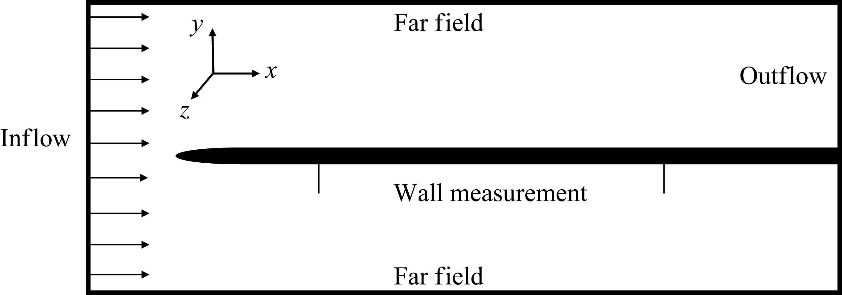
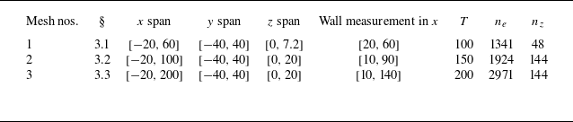
 T
 ne
 x−y
 nz
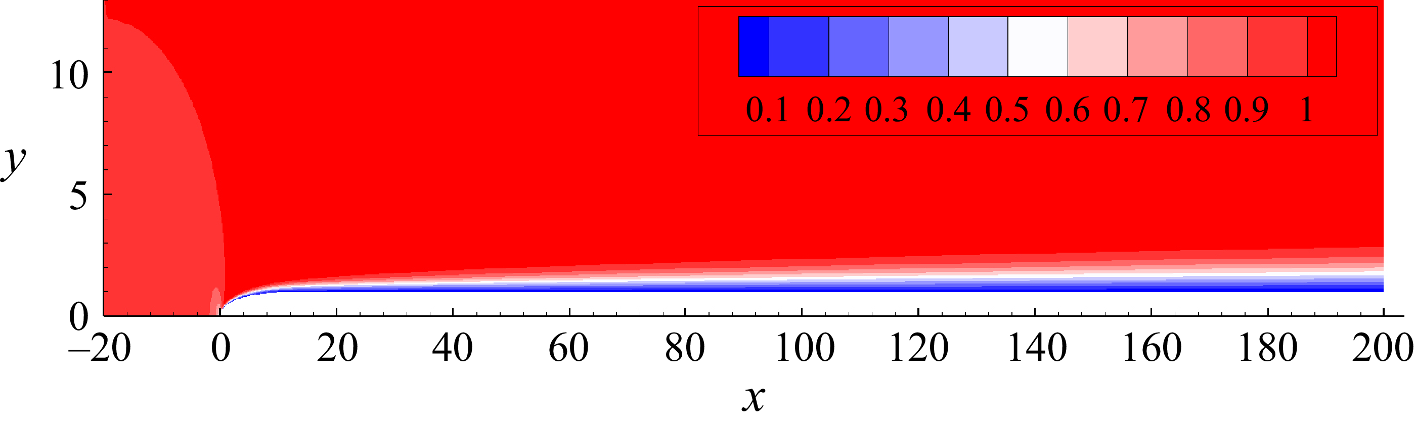
 Re=800
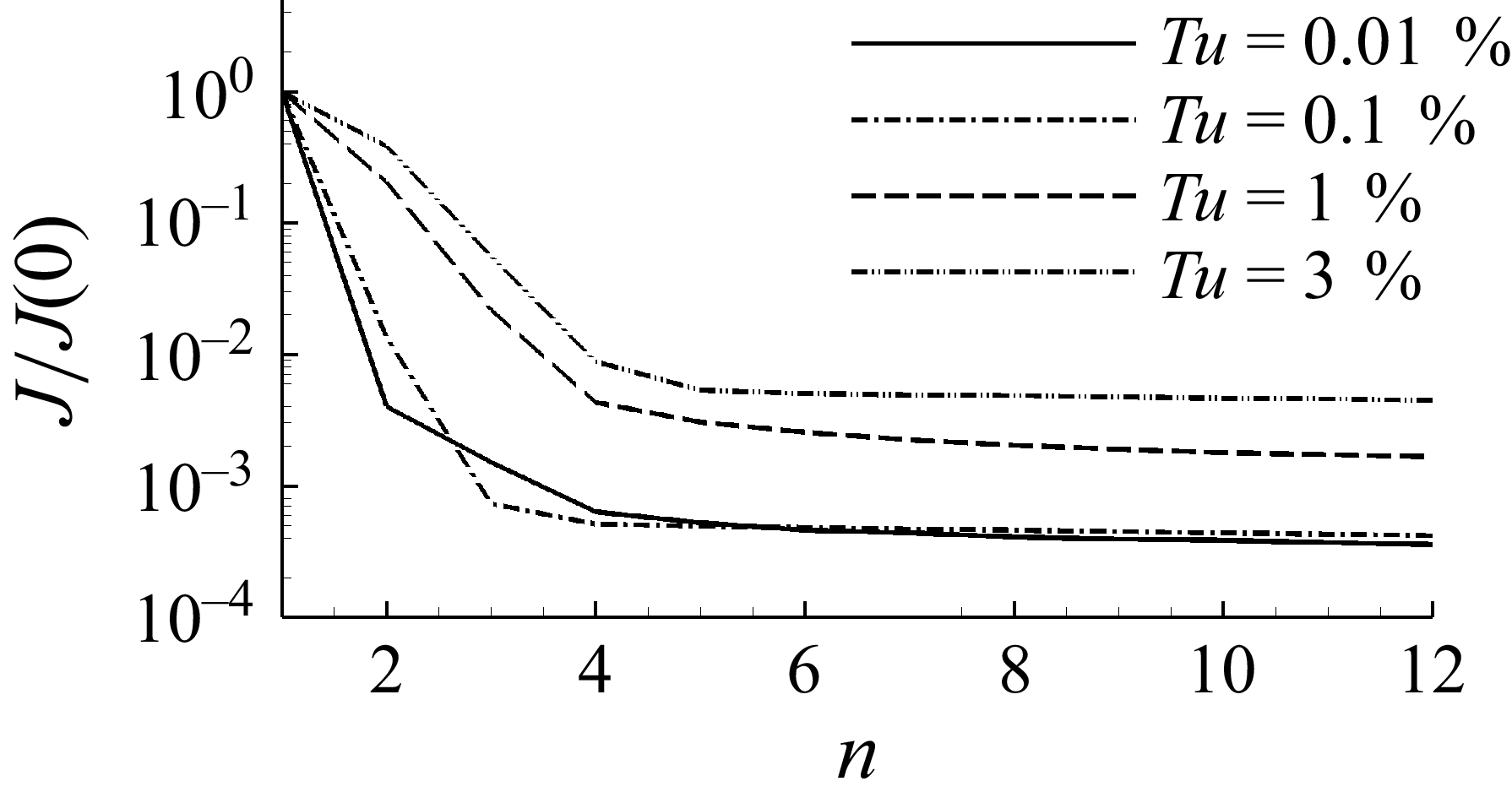
 J
 n

 u′
 x−z
 y−z
 x=50
 Tu=0.01%
 Tu=0.1%
 Tu=1%
 Tu=3%

 Tu=0.1%
 Tu=1%
 Tu=3%

 H^z
 xm=48
 Tu=0.01%
 Tu=0.1%
 Tu=1%
 Tu=3%

 Tu=0.1%
 zm=4.5
 β=1.73
 Tu=1%
 zm=3.5
 β=0
 Tu=1%
 zm=4.5
 β=1.73
 Tu=3%
 zm=3.5
 β=0

 zm
 Tu=0.1%
 zm=4.5
 Tu=3%
 zm=3.6

 Tu=0.1%
 β=1.73
 Tu=3%
 β=0

 u′
 y=1.5
 t=100

 ω=0.026
 ω=0.13

 ein
 ein
 ω=0
 ω
 Tu=1%

 x−z
 y=1.5

 t=0
 x−z
 y=1.5
 T150zero
 T150

 εz
 ∂u/∂y
 T150
 T150zero

 x−z
 y=1.5
 t=200

 v′
 x−z
 t=200
 t=275
 25
 T150
 T200

 u′
 y−z
 t=150
 x=70
 T150
 T200
 t=200
 x=110
 T150
 T200
 u′


