2. DNS, LES and closures

We consider the dimensionless 2-D $\beta$ -plane vorticity equation (e.g. Vallis Reference Vallis2017)

(2.1) \begin{eqnarray} \frac {\partial \omega }{\partial t} +\mathcal{J}(\omega ,\psi ) = \frac {1}{\textit{Re}}\boldsymbol{\nabla} ^2\omega -f-r\omega +\beta \frac {\partial \psi }{\partial x}, \qquad \boldsymbol{\nabla} ^2\psi =-\omega . \end{eqnarray}

Here, $\mathcal{J}$ is the Jacobian, $f(x,y)=k_{\!f}[\cos (k_{\!f}x)+\cos (k_{\!f}y)]$ is a time-independent deterministic forcing at wavenumber $k_{\!f}$ , $\textit{Re}$ is the Reynolds number, $\beta$ is the planetary-vorticity-gradient parameter and $r=0.1$ is the linear friction coefficient.

Applying a sharp spectral cutoff filter, denoted by $\overline {(\boldsymbol{\cdot })}$ , gives the LES or filtered-DNS (FDNS) equation

(2.2) \begin{equation} \frac {\partial \overline {\omega }}{\partial t} +\mathcal{J}(\overline {\omega },\overline {\psi }) = \frac {1}{\textit{Re}}\boldsymbol{\nabla} ^2\overline {\omega } -\overline {f} -r\overline {\omega } +\beta \frac {\partial \overline {\psi }}{\partial x} -\underbrace { \left [ \overline {\mathcal{J}(\omega ,\psi )} - \mathcal{J}(\overline {\omega },\overline {\psi }) \right ] }_{\varPi ^{\textit{SGS}}=\boldsymbol{\nabla }\times (\boldsymbol{\nabla }\boldsymbol{\cdot }\tau ^{\textit{SGS}})}, \; \boldsymbol{\nabla} ^2\overline {\psi }=-\overline {\omega }. \end{equation}

The SGS term $\varPi ^{\textit{SGS}}$ stems from the Jacobian and must be closed in terms of the resolved variables $(\overline {\psi },\overline {\omega })$ . For eddy-viscosity closures,

(2.3) \begin{eqnarray} \tau ^{\textit{SGS}}=-2\nu _e\overline {\mathcal{S}}, \end{eqnarray}

where $\overline {\mathcal{S}}$ is the resolved strain-rate tensor. The Smagorinsky model uses

(2.4) \begin{eqnarray} \nu _e=(C_{{S}}\varDelta )^2 \langle \overline {\mathcal{S}}^2\rangle ^{1/2}, \end{eqnarray}

while the Leith model uses

(2.5) \begin{eqnarray} \nu _e=(C_{{L}}\Delta )^3 \langle (\boldsymbol{\nabla }\overline {\omega })^2\rangle ^{1/2},\quad \text{with} \quad \varDelta =L/N_{\textit{LES}}. \end{eqnarray}

Here, $L=2\pi$ is the domain length, $N_{\textit{LES}}$ is the number of grid points in each direction and $\varDelta$ is the filter width. Additionally, $\langle \boldsymbol{\cdot }\rangle$ denotes domain averaging. The Jansen–Held (JH) closure model is written as

(2.6) \begin{eqnarray} \varPi ^{\textit{SGS}} = \boldsymbol{\nabla} ^2(\nu _e\boldsymbol{\nabla} ^2\overline {\omega }) + \nu _{{B}}\boldsymbol{\nabla} ^2\overline {\omega }, \end{eqnarray}

where the first term dissipates enstrophy through biharmonic eddy viscosity and the second term re-injects energy by anti-diffusion. Similar to their original papers (Jansen & Held Reference Jansen and Held2014; Jansen et al. Reference Jansen, Held, Adcroft and Hallberg2015), we use

(2.7) \begin{eqnarray} \nu _e = (C_{\textit{JH}}\varDelta )^6 \big\langle (\boldsymbol{\nabla} ^2\overline {\omega })^2 \big\rangle ^{1/2}, \quad \nu _{{B}} = -C_{{B}} \frac { \left \langle \overline {\psi }\boldsymbol{\nabla} ^2(\nu _e\boldsymbol{\nabla} ^2\overline {\omega }) \right \rangle }{ \left \langle \overline {\psi }\boldsymbol{\nabla} ^2\overline {\omega } \right \rangle }. \end{eqnarray}

The parameter $C_{{B}}$ prescribes the fraction of dissipated energy re-injected into the resolved scales. Following previous studies (Jansen & Held Reference Jansen and Held2014; Guan et al. Reference Guan, Hassanzadeh, Schneider, Dunbar, Huang, Wu and Lopez-Gomez2026), we set $C_{{B}}=0.95$ in all cases. In the following, we derive the semi-analytical expression for scalar coefficients $C_{{L}}$ , $C_{{S}}$ and $C_{\textit{JH}}$ .

3. Semi-analytical derivation of the closure parameters

The derivation in the following is, to the best of our knowledge, the first Lilly-type global scaling argument for estimating scalar coefficients in commonly used 2-D eddy-viscosity and backscattering closures. We treat the eddy viscosity as spatially uniform, $\nu _e=\nu _e(t)$ , so the resulting coefficients should be interpreted as scalar, domain-averaged closure constants rather than local eddy-viscosity fields. The cutoff condition $\varDelta \sim L_\eta$ is imposed up to a proportionality constant that is absorbed into the closure coefficient. A sharp spectral cutoff, $k_c=\pi /\varDelta$ , is used throughout. Detailed derivations and extensions to a general $k^{-p}$ scaling law are given in the supplementary material.

3.1. $k^{-3}$ spectrum scaling

In 2-D turbulence, the interscale enstrophy transfer is

(3.1) \begin{eqnarray} \eta =\langle \bar {\omega }\varPi \rangle , \end{eqnarray}

where $\eta \gt 0$ denotes transfer from resolved to subgrid or dissipative scales. For an eddy-viscosity closure $\varPi =-\nu _e\boldsymbol{\nabla} ^2\bar {\omega }$ with spatially uniform $\nu _e(t)$ ,

(3.2) \begin{eqnarray} \eta =-\nu _e\langle \bar {\omega }\boldsymbol{\nabla} ^2\bar {\omega }\rangle =\nu _e\langle (\boldsymbol{\nabla }\bar {\omega })^2\rangle . \end{eqnarray}

Requiring $\varDelta$ to resolve the enstrophy-dissipation scale $L_\eta \sim \nu _e^{1/2}\eta ^{-1/6}\sim \nu _e^{1/3} \langle (\boldsymbol{\nabla }\bar {\omega })^2\rangle ^{-1/6}$ (Batchelor Reference Batchelor1969; Boffetta Reference Boffetta2007; Boffetta & Musacchio Reference Boffetta and Musacchio2010) gives the Leith form

(3.3) \begin{eqnarray} \nu _e=(C_{{L}}\Delta )^3\langle (\boldsymbol{\nabla }\bar {\omega })^2\rangle ^{1/2}. \end{eqnarray}

Combining (3.2) and (3.3) yields

(3.4) \begin{eqnarray} \eta =(C_{{L}}\Delta )^3\langle (\boldsymbol{\nabla }\bar {\omega })^2\rangle ^{3/2}. \end{eqnarray}

Using the direct-cascade TKE spectrum

(3.5) \begin{eqnarray} \hat {E}(k)=A\eta ^{2/3}k^{-3} \end{eqnarray}

(Kraichnan Reference Kraichnan1967; Leith Reference Leith1968; Batchelor Reference Batchelor1969) and Parseval’s theorem,

(3.6) \begin{eqnarray} \langle (\boldsymbol{\nabla }\bar {\omega })^2\rangle =2\int _0^{k_c}k^4\hat {E}(k)\,{\rm d}k =A\eta ^{2/3}k_c^2, \end{eqnarray}

where $k_c=\pi /\varDelta$ . Here and in the following, the scaling law is applied to the FDNS spectrum up to $k_c$ . For moments dominated by high wavenumbers, the error from extending the direct-cascade form below $k_{\!f}$ is assumed small. Substitution into (3.4) gives

(3.7) \begin{eqnarray} C_{{L}}=\pi ^{-1} A^{-1/2}. \end{eqnarray}

To the best of our knowledge, (3.7) gives the first explicit relation between a 2-D LES closure coefficient and the amplitude of an enstrophy-cascade scaling law. In the following, the same framework is extended to Smagorinsky, biharmonic eddy-viscosity and JH backscattering closures. For the biharmonic eddy-viscosity part of the JH closure, setting $C_{{B}}=0$ ,

(3.8) \begin{eqnarray} \eta =\nu _e\langle \bar {\omega }{\nabla} ^4\bar {\omega }\rangle =\nu _e\langle (\boldsymbol{\nabla} ^2\bar {\omega })^2\rangle , \qquad \nu _e=(C_{\textit{JH}}\Delta )^6 \langle (\boldsymbol{\nabla} ^2\bar {\omega })^2\rangle ^{1/2}. \end{eqnarray}

The corresponding spectral moment is

(3.9) \begin{eqnarray} \langle (\boldsymbol{\nabla} ^2\bar {\omega })^2\rangle =2\int _0^{k_c}k^4\hat {Z}(k)\,{\rm d}k =\frac {A}{2}\eta ^{2/3}k_c^4, \end{eqnarray}

where $\hat {Z}(k)=k^2\hat {E}(k)$ is the enstrophy spectrum. Substituting back into (3.8) and using $k_c=\pi /\varDelta$ gives

(3.10) \begin{eqnarray} C_{\textit{JH}}=(A/2)^{-1/4}\pi ^{-1}. \end{eqnarray}

In general, for a $2m$ -order eddy-viscosity model ( $\varPi =(-1)^{m}\nu _e{\nabla} ^{2m}\bar {\omega }$ and $\nu _e=(C_m\Delta )^{3m} \langle ({\nabla} ^m\bar {\omega })^2\rangle ^{1/2}$ ), the model coefficient can be derived as $C_m= (A/m)^{-1/(2m)}/\pi$ . As discussed by Kitsios et al. (Reference Kitsios, Frederiksen and Zidikheri2013), higher $k_c$ may favour a higher-order operator.

For the full JH model with a prescribed $C_{{B}}$ , using (2.6) in (3.2) gives

(3.11) \begin{eqnarray} \eta =(C_{\textit{JH}}\Delta )^6(A/2)^{3/2}\eta k_c^6 -\nu _{{B}}A\eta ^{2/3}k_c^2. \end{eqnarray}

From (2.7),

(3.12) \begin{eqnarray} \nu _{{B}} =C_{{B}}\nu _e \frac {2\int _0^{k_c}k^2\hat {Z}(k)\,{\rm d}k} {2\int _0^{k_c}\hat {Z}(k)\,{\rm d}k} \approx C_{{B}}\nu _e\frac {k_c^2}{2\ln (k_c)} , \end{eqnarray}

where the denominator is evaluated from the smallest nonzero wavenumber, $k=1$ , in the $2\pi$ -periodic domain. This logarithmic factor introduces a weak dependence on the large-scale cutoff and on the sharp-filter convention. Substituting (3.12) into (3.11) gives

(3.13) \begin{eqnarray} C_{\textit{JH}} =(A/2)^{-1/4}\pi ^{-1} \left (1-\frac {C_{{B}}}{\ln (k_c)}\right )^{-1/6}. \end{eqnarray}

Finally, we estimate $C_{{S}}$ by matching the globally averaged Smagorinsky and Leith eddy viscosities for a resolved field with the assumed spectrum:

(3.14) \begin{eqnarray} (C_{{L}}\varDelta )^3\langle (\boldsymbol{\nabla }\bar {\omega })^2\rangle ^{1/2} =(C_{{S}}\varDelta )^2\langle \bar {\mathcal{S}}^2\rangle ^{1/2}. \end{eqnarray}

With

(3.15) \begin{eqnarray} \langle \bar {\mathcal{S}}^2\rangle =2\int _0^{k_c}k^2\hat {E}(k)\,{\rm d}k \approx 2A\eta ^{2/3}\ln (k_c), \end{eqnarray}

we obtain

(3.16) \begin{eqnarray} C_{{S}}=A^{-3/4}\pi ^{-1}(2\ln (k_c))^{-1/4}. \end{eqnarray}

Equations (3.7), (3.13) and (3.16) give semi-analytical expressions for the Leith, JH and Smagorinsky coefficients under the classical $k^{-3}$ enstrophy-cascade scaling, all determined up to the amplitude constant $A$ . To the best of our knowledge, this provides the first explicit scaling-based estimate of these commonly used 2-D LES closure coefficients. We next repeat the derivation using the logarithmically corrected $k^{-3}$ spectrum.

3.2. $k^{-3}{[\ln (k/k_{\!f})]}^{-1/3}$ spectrum scaling

For the logarithmically corrected direct-cascade spectrum (Kraichnan Reference Kraichnan1971)

(3.17) \begin{eqnarray} \hat {E}(k)=A'\eta ^{2/3}k^{-3}[\ln (k/k_{\!f})]^{-1/3}, \end{eqnarray}

the scaling is applied only for $k\gt k_{\!f}$ ; in the discrete spectra, we therefore use $k_{\!f}+1$ as the lower limit. The leading-order spectral moments are

(3.18) \begin{eqnarray} \langle (\boldsymbol{\nabla }\bar {\omega })^2\rangle &\approx & 2\int _{k_{\!f}+1}^{k_c} A'\eta ^{2/3}k[\ln (k/k_{\!f})]^{-1/3}\,{\rm d}k \nonumber \\[3pt] &\approx & A'\eta ^{2/3}k_c^2[\ln (k_c/k_{\!f})]^{-1/3} \end{eqnarray}

and

(3.19) \begin{eqnarray} \langle (\boldsymbol{\nabla} ^2\bar {\omega })^2\rangle &\approx & 2\int _{k_{\!f}+1}^{k_c} A'\eta ^{2/3}k^3[\ln (k/k_{\!f})]^{-1/3}\,{\rm d}k \nonumber \\[3pt] &\approx & \frac {A'}{2}\eta ^{2/3}k_c^4[\ln (k_c/k_{\!f})]^{-1/3}. \end{eqnarray}

These approximations follow from the slow variation of the logarithmic factor or, equivalently, from Karamata’s theorem (Bingham et al. Reference Bingham, Goldie and Teugels1989). Repeating the above-mentioned balances gives

(3.20) \begin{equation} C'_{{L}} =\frac {1}{\pi A'^{1/2}}[\ln (k_c/k_{\!f})]^{1/6}, \end{equation}

(3.21) \begin{equation} C'_{\textit{JH}} =(A'/2)^{-1/4}\pi ^{-1}[\ln (k_c/k_{\!f})]^{1/12}. \end{equation}

Here, we use $C'_{{L}}$ and $C'_{\textit{JH}}$ with $'$ to denote coefficients derived from the logarithmically corrected direct-cascade spectrum. For a prescribed $C_{{B}}$ , the same asymptotic estimate gives $\nu _{{B}}\approx (C_{{B}}/3)\nu _e k_c^2[\ln (k_c/k_{\!f})]^{-1}$ , leading to

(3.22) \begin{eqnarray} C'_{\textit{JH}} =(A'/2)^{-1/4}\pi ^{-1}[\ln (k_c/k_{\!f})]^{1/12} \left (1-\frac {2C_{{B}}}{3\ln (k_c/k_{\!f})}\right )^{-1/6}. \end{eqnarray}

Similarly, matching the globally averaged Smagorinsky and Leith eddy viscosities yields

(3.23) \begin{eqnarray} C'_{{S}}=3^{-1/4}A'^{-3/4}\pi ^{-1}. \end{eqnarray}

Figure 1.

TKE spectra ( $\hat {E}(k)$ ) and examples of $\omega$ for representative Cases 1.1, 2.1 and 3. The $k_{\!f}$ and $k_c$ are marked. The black curves show DNS spectra averaged over 100 snapshots. The red (blue) dashed line shows the $k^{-3}$ scaling law (with logarithmic correction), with the $A$ ( $A'$ ) values shown in table 1. The orange dashed line shows the effective $k^{-4}$ scaling law for Case 3 only. With a sharp spectral cutoff filter, the FDNS spectrum overlaps with the DNS spectrum over $k\in [0,k_c]$ .

Figure 1. Long description

Figure 1 compares representative cases 1.1, 2.1, and 3. For each case, the figure shows the turbulent kinetic energy spectrum and an example vorticity field. The forcing wavenumber and cutoff wavenumber are marked on the spectra. DNS spectra are averaged over 100 snapshots. Reference curves show the classical k to the minus 3 scaling, the logarithmically corrected k to the minus 3 scaling, and, for the anisotropic beta-plane Case 3 only, an effective k to the minus 4 scaling. With the sharp spectral cutoff filter, the FDNS spectrum overlaps the DNS spectrum up to the cutoff wavenumber.

3.3. Effective $k^{-4}$ scaling for the $\beta$ -plane case

For the anisotropic $\beta$ -plane case considered in the following, the angle-integrated TKE spectrum is steeper than the classical $k^{-3}$ direct-cascade spectrum, as shown in figure 1. We therefore also use an effective $k^{-4}$ scaling,

(3.24) \begin{eqnarray} \hat {E}(k)=A''\eta ^{2/3}k_* k^{-4}, \end{eqnarray}

where $k_*$ is a characteristic wavenumber used to keep $A''$ dimensionless and the choice of $k_*$ will affect the value of $A''$ , but will not affect the derived closure coefficients. Following the same arguments and assumptions as before, and using the leading-order spectral moments

(3.25) \begin{eqnarray} \langle (\boldsymbol{\nabla }\bar {\omega })^2\rangle \approx 2A''\eta ^{2/3}k_* k_c, \qquad \langle (\boldsymbol{\nabla} ^2\bar {\omega })^2\rangle \approx \frac {2A''}{3}\eta ^{2/3}k_* k_c^3, \end{eqnarray}

we obtain the Leith coefficient and JH coefficient with prescribed $C_{{B}}$ :

(3.26) \begin{equation} C''_{{L}} = \frac {1}{\pi } \left (\frac {k_c}{2A''k_*}\right )^{1/2},\quad C''_{\textit{JH}} = \frac {1}{\pi } \left (\frac {2A''k_*}{3}\right )^{-1/4} k_c^{1/4} \left (1-\frac {3C_{{B}}{ k_1}}{k_c}\right )^{-1/6}\!. \end{equation}

Here, $k_1$ denotes the lowest nonzero wavenumber and equals $1$ in a $2\pi \times 2\pi$ computational domain. We use $C''_{{L}}$ and $C''_{\textit{JH}}$ with $''$ to denote coefficients derived from the effective $k^{-4}$ scaling. These expressions are used only as an effective isotropic representation of the angle-integrated spectrum in the anisotropic $\beta$ -plane case. The corresponding $C_{{S}}''$ involves a strain moment that is dominated by $k_1$ , and it is more sensitive to the chosen fitting range than the Leith and biharmonic estimates. Therefore, it is not used as a primary coefficient estimate.

Table 1.

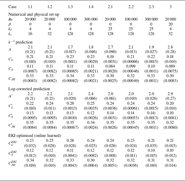
Physical and numerical parameters of the eight cases and comparison between semi-analytical predictions and EKI-optimised coefficients. The semi-analytical predictions are obtained using either the $k^{-3}$ scaling or the logarithmically corrected $k^{-3}[\ln (k/k_{\!f})]^{-1/3}$ scaling. Values in parentheses denote one standard deviation over the 100 DNS TKE spectra. For the JH closure, $C_{\textit{JH}}$ is estimated with $C_{{B}}=0.95$ for all semi-analytical predictions. For the anisotropic $\beta$ -plane Case 3, the effective $k^{-4}$ scaling predicts $C_{{L}}''=0.18 (0.0079)$ and $C_{\textit{JH}}''=0.32 (0.0070)$ . The DNS and LES set-up details, and the derivation of $C_{{S}}''$ (not used as primary estimate) are in the supplementary material.

Table 1. Long description

Table 1 summarizes eight 2D turbulence cases: Cases 1.1 to 1.4, Cases 2.1 to 2.3, and Case 3. It lists Reynolds number, beta, forcing wavenumber, and cutoff wavenumber, followed by semi-analytical predictions from the k to the minus 3 spectrum and from the logarithmically corrected k to the minus 3 spectrum. The listed coefficients are the Leith, Smagorinsky, and Jansen-Held coefficients, with one standard deviation over 100 DNS spectra shown in parentheses. The table also reports EKI-optimized coefficients from prior online learning. The values show that the semi-analytical predictions are generally close to the EKI-optimized coefficients. For anisotropic beta-plane Case 3, the effective k to the minus 4 scaling predicts C double-prime sub L equal to 0.18 with standard deviation 0.0079, and C double-prime sub JH equal to 0.32 with standard deviation 0.0070.

4. Numerical results

To evaluate the semi-analytical estimates of $C_{{L}}$ , $C_{\textit{JH}}$ and $C_{{S}}$ , we use the DNS and LES datasets generated by Guan et al. (Reference Guan, Hassanzadeh, Schneider, Dunbar, Huang, Wu and Lopez-Gomez2026). The physical and numerical parameters of the eight cases are summarised in table 1. The DNS TKE spectra and representative vorticity fields for three cases are shown in figure 1. Table 1 also reports the diagnosed amplitudes $A$ and $A'$ obtained by fitting $\hat {E}(k)=A\eta ^{2/3}k^{-3}$ and $\hat {E}(k)=A'\eta ^{2/3}k^{-3}[\ln (k/k_{\!f})]^{-1/3}$ to the direct-cascade range $k\in [k_{\!f}+1,k_\eta ]$ of the DNS TKE spectra. In 2-D turbulence, the enstrophy-cascade dissipation wavenumber scales as $k_{\textit{diss}}\sim \nu ^{-1/2}\eta ^{1/6}\sim \textit{Re}^{1/2}\eta ^{1/6}$ (Boffetta Reference Boffetta2007; Boffetta & Musacchio Reference Boffetta and Musacchio2010). To avoid fitting the viscous-dissipation range, we set the fitting upper bound to $k_\eta =\xi \textit{Re}^{1/2}\eta ^{1/6}$ with $\xi =0.25$ . Here, $\xi$ is a fitting-range parameter, chosen conservatively and tested by sensitivity analysis in the supplementary material available at https://doi.org/10.1017/jfm.2026.12056. The enstrophy dissipation rate is diagnosed from the same DNS TKE spectra as (Davidson Reference Davidson2015)

(4.1) \begin{equation} \eta =\langle (\boldsymbol{\nabla }\omega )^2\rangle /\textit{Re}=\frac {2}{\textit{Re}}\int _0^{k_{\textit{DNS}}} k^4 \hat {E}(k)\,{\rm d}k. \end{equation}

After the flow reaches statistical equilibrium, the snapshot-averaged spectrum and the diagnosed mean $\eta$ are statistically stationary. The TKE spectrum is calculated by averaging spectra from 100 decorrelated DNS snapshots. As discussed by Guan et al. (Reference Guan, Hassanzadeh, Schneider, Dunbar, Huang, Wu and Lopez-Gomez2026), even one snapshot can be sufficient for estimating $A$ and $A'$ accurately. Except for Case 3, $A$ and $A'$ are nearly flow independent and are both close to $2$ . The somewhat larger $A$ in Case 2.1 is likely related to the shorter available fitting interval between $k_{\!f}+1$ and $k_\eta$ , making the original $k^{-3}$ scaling more sensitive to the selected fitting upper bound. This motivates the log-corrected scaling, which shows reduced sensitivity to $\xi$ in the supplementary material. The diagnosed values of $A'$ are close to the mode-coupling estimates of the log-corrected 2-D enstrophy-cascade spectral constant reported by Nandy & Bhattacharjee (Reference Nandy and Bhattacharjee1995), including the corrected one-loop value $1.923$ and the self-consistent value $2.201$ , and are broadly consistent with other theoretical estimates based on test-field closure approximation and renormalisation-group methods (e.g. Kraichnan Reference Kraichnan1971; Olla Reference Olla1991). The diagnosed $A$ values are consistent with empirical effective $k^{-3}$ amplitudes reported in 2-D turbulence (e.g. Boffetta & Ecke Reference Boffetta and Ecke2012; Gupta et al. Reference Gupta, Jayaram, Chaterjee, Sadhukhan, Samtaney and Verma2019). Case 3 has larger fitted amplitudes ( $A=2.8$ and $A'=2.9$ ), likely due to the strong anisotropy and jet-like structures induced by the $\beta$ effect. As shown in figure 1, the $k^{-3}$ and log-corrected $k^{-3}$ spectra are too shallow for this case. We therefore also consider an effective $k^{-4}$ scaling of the angle-integrated spectrum for Case 3. This scaling should be interpreted as an empirical isotropic representation of the steepened spectrum in the anisotropic $\beta$ -plane case, rather than as a universal $\beta$ -plane scaling law (e.g. Rhines Reference Rhines1975; Galperin et al. Reference Galperin, Sukoriansky and Dikovskaya2008, Reference Galperin, Sukoriansky and Dikovskaya2010; Sukoriansky et al. Reference Sukoriansky, Dikovskaya and Galperin2009). Physically, the imposed planetary vorticity gradient supports Rossby-wave dynamics and anisotropic jet-like organisation, which redistribute energy towards large-scale zonal modes and weaken the assumptions of a $k^{-3}$ enstrophy cascade. Here, the $k^{-4}$ estimation is intended as a consistency check showing how the coefficient-estimation framework changes for a steeper observed spectrum, rather than as evidence of improvement. Since only one anisotropic case is considered, universality of the effective exponent and amplitude in anisotropic regimes is left for future work.

Overall, the semi-analytical estimates of $C_{{L}}$ , $C_{\textit{JH}}$ and $C_{{S}}$ agree well with the EKI-optimised values of Guan et al. (Reference Guan, Hassanzadeh, Schneider, Dunbar, Huang, Wu and Lopez-Gomez2026). This agreement provides an independent validation of the semi-analytical approach and, furthermore, shows that the EKI-optimised parameters can be interpreted through classical 2-D turbulence scaling. LES results using the semi-analytically estimated parameters for three representative cases are shown in figure 2. These cases are selected to represent distinct regimes and to include cases where the semi-analytical predictions deviate most from the EKI-optimised values. In a posteriori tests based on TKE spectra and vorticity probability density functions, LES with the semi-analytical parameters robustly outperform the dynamic Leith (Maulik & San Reference Maulik and San2016) and dynamic Smagorinsky (Germano et al. Reference Germano, Piomelli, Moin and Cabot1991) baselines, particularly in the probability density function (p.d.f.) tails (additional implementation details are provided in the supplementary material). The backscattering JH closures better capture the tails of the FDNS vorticity p.d.f.s than purely diffusive closures.

Figure 2.

A posteriori testing with semi-analytical model parameters shown in table 1. (a) TKE spectra ( $\hat {E}(k)$ ) comparison among the ground truth (FDNS), baseline models (dynamic Leith, or DLeith, and dynamic Smagorinsky, or DSmag) and the semi-analytical models derived from the $k^{-3}$ scaling (with $C_{{L}}$ or $C_{\textit{JH}}$ ), and the logarithmic correction (with $C'_{{L}}$ or $C'_{\textit{JH}}$ ), for representative Cases 1.1, 2.1 and 3. The semi-analytical models show a better match with the ground truth than DSmag among all three cases and better than DLeith in Case 3. (b) Positive tail of the vorticity probability density function, $\mathcal{P}(\omega )$ . The negative tail gives the same qualitative conclusions because the vorticity is nearly symmetric about zero. The semi-analytical JH models consistently match the FDNS $\mathcal{P}(\omega )$ within 1 standard deviation (grey shaded area), especially in the tails or rare extreme events. The semi-analytical Leith models, although not as accurate as the JH models, outperform the baseline models. The mild high- $k$ curl-up of Case 2.1 $\hat {E}(k)$ may be improved with a higher-order operator with an estimated $C_m$ .

Figure 2. Long description

Figure 2 shows a posteriori LES testing for representative cases 1.1, 2.1, and 3 using the semi-analytical model parameters reported in Table 1. The first row compares turbulent kinetic energy spectra from FDNS, dynamic Leith, dynamic Smagorinsky, and semi-analytical Leith and Jansen-Held models derived from the k to the minus 3 scaling and from the logarithmically corrected scaling. The second row compares the positive tails of the vorticity probability density function. The semi-analytical models match the FDNS spectra better than dynamic Smagorinsky in all three cases and better than dynamic Leith in Case 3. The semi-analytical Jansen-Held models consistently match the FDNS vorticity PDFs within one standard deviation, especially in the tails or rare-event region. The semi-analytical Leith models are less accurate than Jansen-Held but still outperform the dynamic baselines. Case 2.1 shows a mild high-wavenumber curl-up in the spectrum that may be improved by a higher-order operator.

5. Summary and conclusion

We have developed semi-analytical estimates for the scalar coefficients in the Leith, Smagorinsky and Jansen–Held closures for 2-D geophysical turbulence. The derivation extends a Lilly-type global scaling argument to 2-D turbulence and uses either the classical $k^{-3}$ direct-cascade spectrum or its log-corrected form above the forcing scale.

The estimates depend on an amplitude constant, e.g. $A$ or $A'$ , and are therefore semi-analytical rather than fully analytical. For $\beta =0$ cases, however, the diagnosed amplitudes are nearly case-independent. Specifically, the log-corrected amplitude is consistent with previous theoretical estimates based on test-field closure approximations, renormalisation-group analysis, and mode-coupling theory. The resulting closure coefficients agree well with the EKI-optimised parameters obtained in our online-learning study (Guan et al. Reference Guan, Hassanzadeh, Schneider, Dunbar, Huang, Wu and Lopez-Gomez2026).

A posteriori LES tests show that closures using the semi-analytical parameters reproduce key DNS statistics and compare favourably with dynamic Leith and Smagorinsky baselines, especially in the vorticity-p.d.f. tails. For the anisotropic $\beta$ -plane case, the angle-integrated spectrum is steeper and is better represented by an effective $k^{-4}$ scaling, which should be viewed as a first approximation rather than a universal $\beta$ -plane law. Future work will test these coefficients in more realistic geophysical models and develop an anisotropic theory for $\beta$ -plane regimes with a sweep on $\textit{Re}$ , $k_{\!f}$ , etc. More broadly, together with the EKI results of Guan et al. (Reference Guan, Hassanzadeh, Schneider, Dunbar, Huang, Wu and Lopez-Gomez2026), this work illustrates how modern data-driven closure discovery can motivate, guide and validate new theoretical developments in turbulence modelling.