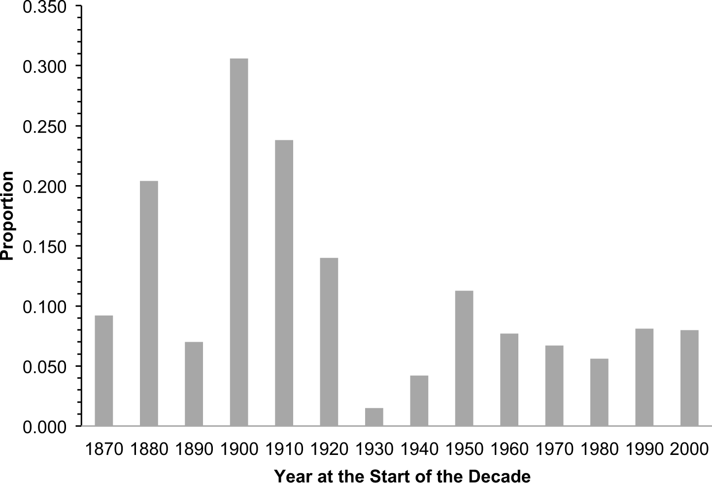
The 1910s and 1920s were, respectively, the second and fourth largest immigrant inflow decades in Canadian history in per capita terms. Between 1911 and 1920, an immigrant inflow amounting to approximately 24 percent of Canada's 1911 population arrived in Canada, and between 1921 and 1930, the inflow equaled 14 percent of the 1921 population. In comparison, the largest immigrant decade (in a proportional sense) for the United States since Canadian Confederation in 1867 was the decade from 1900 to 1909 when immigrant inflows totaled 11 percent of the 1900 U.S. population.Footnote 1 For Canada, the inflows in the 1910s and 1920s were accompanied by large emigration to the United States, and we discuss this as part of immigrant adjustment after arrival, but even after accounting for that, immigrants who arrived in the previous decade made up 17 percent of male employment in 1921 and 14 percent in 1931.Footnote 2 Those percentages are at least double the size of the Mariel Boatlift inflow to the Miami labour market in the 1980s that has been the focus of considerable attention in discussions of immigration impacts in modern economies (Card Reference Card1990), and are two to three times the proportion of the Canadian population in 2006 who had arrived in the previous decade (6.2 percent). Moreover, in 1931, 38 percent of male wage earners in Canada were foreign born. Thus, whatever measures we use, Canada received substantial immigration inflows in the 1910s and 1920s. These large inflow decades were then followed by the lowest immigrant inflow decade on record: the 1930s.
We will show that this large influx and then almost complete cessation of immigration coincided with a substantial change in the Canadian earnings structure. Between 1910 and 1930, the ratio of the 90th to the 10th percentiles of the male annual earnings distribution increased by nearly 50 percent before experiencing a slight decline between 1930 and 1940. Our primary goal in this article is to investigate the contribution of the large and variable immigrant inflow to the changes in the Canadian earnings structure between 1910 and 1940. That is, we are interested in the counterfactual question of how different the earnings structure would have been in the absence of immigration. We do this, first, using a decomposition technique, which shows the direct impact of immigrants on the earnings distribution in the absence of general equilibrium effects. We then estimate the impact of immigration on the earnings of the native born and previously arrived immigrants within the context of a nested Constant Elasticity of Substitution (CES) model of production that allows for broader, general equilibrium effects of immigration. In estimating that model, we address potential endogeneity concerns arising because the immigration inflows were not exogenous shocks but were distributed across occupations partly in response to demand patterns arising from demand for Canadian exports, technological change, etc. In particular, we use an ethnic enclave instrument that takes advantage of the fact that new immigrants tend to locate where previous immigrants from their source country are living. Perhaps surprisingly, we find that the immigrant inflows had some effects on low skilled earnings but very limited effects on the overall shape of the earnings distribution. While there are studies of the effect of the set of changes the Canadian economy experienced on average wages in Canada in this period (e.g., Lewis Reference Lewis1975), to the best of our knowledge, there is no prior empirical analysis of the impact of the large pre-WWII immigrant inflows into Canada on its earnings structure.
Following from this first result, our second goal is to examine why such a large inflow would have such apparently small impacts on the earnings distribution. The first main reason is because of immigrant adaptation. As Ran Abramitzky, Leah Platt Boustan, and Katherine Eriksson (Reference Abramitzky, Boustan and Eriksson2014) emphasize, in periods with laissez-faire immigration policy, one might expect that it is mainly potential immigrants with skills that match demands in the host country economy who will actually migrate. This would be reflected in occupation distributions of new immigrants being similar to those of the native born and earlier arrivals. This is what Abramitzky et al. (Reference Abramitzky, Boustan and Eriksson2014) find for the United States in the era of mass migration. For Canada, the federal government had limited ability to control anything, including the total level of immigration, in the period before WWI, and we find that the occupational distribution of new immigrants was similar to that of the native born. This fits with the findings in Alan G. Green and David A. Green (Reference Green1993) using data from manifests of ships arriving at Canada in 1912. To the extent that the occupational distribution of recent immigrants was similar to that of the native born and previously arrived immigrants, one would expect immigration to affect the level of earnings but not the shape of the earnings distribution.
Immigrants also made substantial occupational adjustments after arrival. Compared to their statements about intended occupations at the time of landing, immigrants were ultimately much less likely to be employed in agricultural labourer jobs and more likely to be in clerical and general labourer jobs. These post-arrival adjustments were important in all decades but were particularly important in the 1920s—a decade when Canada had adopted a more activist immigration policy that helped generate an inflow dominated by farmers and farm labourers. Immigrants made the adjustment through a variety of channels: re-migration (often to the United States); geographic migration within Canada; and switching occupations. We cannot distinguish the relative importance of these channels but we show that approximately two-thirds of immigrants arriving in the late 1920s were working in Canada at the time of the 1931 Census and so immigrants did not merely pass through Canada without impacting the Canadian labour market. But whatever the form of the adjustment, the net effect was an occupational distribution that looked quite similar to that of the native born within ten years of an immigrant cohort arriving. Again, this implies a limited impact of immigration on the shape of the earnings distribution. This result fits with arguments in Christian Dustmann and Ian Preston (2012) that one needs to be clear on where immigrants actually end up working in an economy to understand their impact on wages. In addition, our estimates imply general equilibrium adjustments in response to the immigrant supply shocks.
We investigate the ultimate impact of immigration on the earnings structure by working with the estimates of the parameters of our model of production to construct a set of counterfactual exercises. We find that a counterfactual scenario with no immigrants entering Canada in the 1920s implies small effects on both the level and spread of the native-born earnings distribution. In contrast, a policy that blocked only agricultural and general labourers from entering Canada in the 1920s would have increased earnings below the 40th percentile of the native-born distribution by about 10 percent and reduced the increase in inequality in this decade by one-third. Focusing on farm labour (the main immigrant group among males), we show that their annual earnings would have fallen by 42 percent over the 1920s if all immigrant arrivals during that decade had stayed in Canada and in their stated intended occupation at time of arrival. Once we allow for the post-arrival adjustments by the immigrants themselves that impact is reduced to 13 percent, and once we allow for general equilibrium effects, it is further reduced to a 4 percent decline. We conclude, much as earlier discussions that incorporate full general equilibrium effects (e.g., Hatton and Williamson Reference Hatton and Jeffrey G.1998) that immigration inflows within an occupation can have substantial impacts on wages in that occupation if the inflows are viewed in isolation. But once we take account of spillover effects through patterns of substitutability across occupations and of the fact that immigration inflows are either more balanced at arrival than is typically recognized or become more balanced with time in the host economy, the net impact on earnings inequality is limited.
As part of investigating the impact of immigration on the earnings distribution, we document movements in Canadian earnings inequality in the first half of the twentieth century. We see this as a central contribution of the article. To document movements in the Canadian earnings distribution, we use recently available micro data from the decadal Censuses of 1911, 1921, 1931, and 1941. The key advantage of this data is that it includes consistent questions on earnings across these Censuses. Working with this, we document large increases in inequality in the 1920s that were previously undocumented and also show new patterns in terms of experience profiles by occupation and intra-occupation changes in inequality. Our results are broader than those in earlier articles that either used aggregate wage data or relate only to a few occupations in the construction and manufacturing trades plus labourers (Bertram and Percy Reference Bertram and Michael B.1979; Mackinnon Reference Mackinnon1996; Emery and Levitt Reference Emery and Levitt2002). We document a decadal pattern in which wage and earnings inequality changed little between 1910/11 and 1920/21, increased sharply between 1920/21 and 1930/31, then declined somewhat between 1930/31 and 1940/41. The net result was a substantial increase in inequality across the period stretching from just before WWI to just before WWII. The main implication from our estimates of immigration impacts is that the large increase in earnings inequality in the 1920s was not primarily due to immigration and must, instead, have reflected other forces relating to technological change, institutional change, or trade.
Immigration Policy and Patterns
We begin with an overview of Canadian immigration policy before WWII, which will form the basis for our argument that changes in that policy helped determine how immigrants adapted to the Canadian economy. Green (Reference Green1993), in a discussion of the political economy of immigration policy in Canada from 1896 to 1930, shows that the period can be divided into two periods: a period with a more laissez faire policy before WWI and a period with a more actively selective policy after WWI. He argues that the central theme of Canadian economics policy from Confederation in 1867 to WWI (and, possibly, into the 1920s) was the settlement of the West. In this context, immigration directed to the West was seen as having benefits both in providing a market for the burgeoning manufacturing sector in Central and Eastern Canada and in keeping the West safe from American expansionism. To carry it out, the Departments of Agriculture and the Interior established immigrant agents in the United States, Britain, and to a limited extent, Continental Europe whose job was to attract farmers and farm workers who would be willing to settle in the West. Importantly, before 1906 there was no legislation in place to allow the government to refuse immigrants apart from “the diseased, the criminal or vicious, and those likely to become public charges” (Green Reference Green1993).Footnote 3
The shift to a selective immigration policy began with revisions to the Immigration Act in 1906, but the real watershed was the new Act introduced in 1910. The key section in the 1910 Act allowed the government to prohibit immigrants from landing if they belonged to “any race deemed unsuited to the climate or requirements of Canada,” or in any specified class, occupation, or character. Further, these prohibitions could be implemented through regulations, without the need to go to Parliament for approval (Kelley and Trebilcock Reference Kelley and Trebilcock2010). The government now had almost unlimited power to select exactly the immigrants they wanted. It was a power they did not use to any real extent before WWI but it was used afterwards (Green Reference Green1993).
Green (Reference Green, Hatton and Williamson1994) argues that WWI was also a watershed in the role the West played in Canadian economic growth. Between the closing of the American frontier in 1896 and 1914, the expansion into the unsettled lands of the Prairies induced an unprecedented investment boom. But it was after WWI that Western exports of grains truly began to contribute as a driver of economic growth. In the new phase, too, there was strong demand for labour in the West. Partly this was because there was still land to be filled (Lew Reference Lew2000), but it was also because the farm export sector needed labour for its highly seasonal production cycle.
Canada's immigration policy in the 1920s, like that in the United States, distinguished between preferred countries (essentially, Britain, the United States, and Northern and Western Europe), less preferred countries (Southern and Eastern Europe), and more or less prohibited countries (Asia). Prospective immigrants from preferred countries faced virtually no restrictions. Those from non-preferred countries were only to be admitted if they were farmers or farm labourers or, if they were women, domestic servants. Unlike the United States, Canada did not impose numerical quotas to enforce this policy. Instead, Green (Reference Green1993) argues, control was carried out indirectly by the requirement that immigrants from countries other than Britain had to get a visa before entering Canada in conjunction with the strategic placement of visa offices in preferred as opposed to non-preferred countries. This policy combination on its own would likely have created an immigration inflow much like that in the United States in the 1920s—small relative to the pre-war period and mainly from preferred countries (Lew Reference Lew2000). However, in 1925, the Canadian government entered into agreements with the two main railway companies for them to recruit agricultural labour in non-preferred countries. Byron Lew (Reference Lew2000) shows that in the remaining years of the 1920s there was a substantial composition shift in immigration toward immigrants from the non-preferred countries of Europe and headed for the West.Footnote 4 Finally, with the onset of the Depression, the Canadian government used its powers to all but shut down immigration.
Immigration: Flows and Stocks
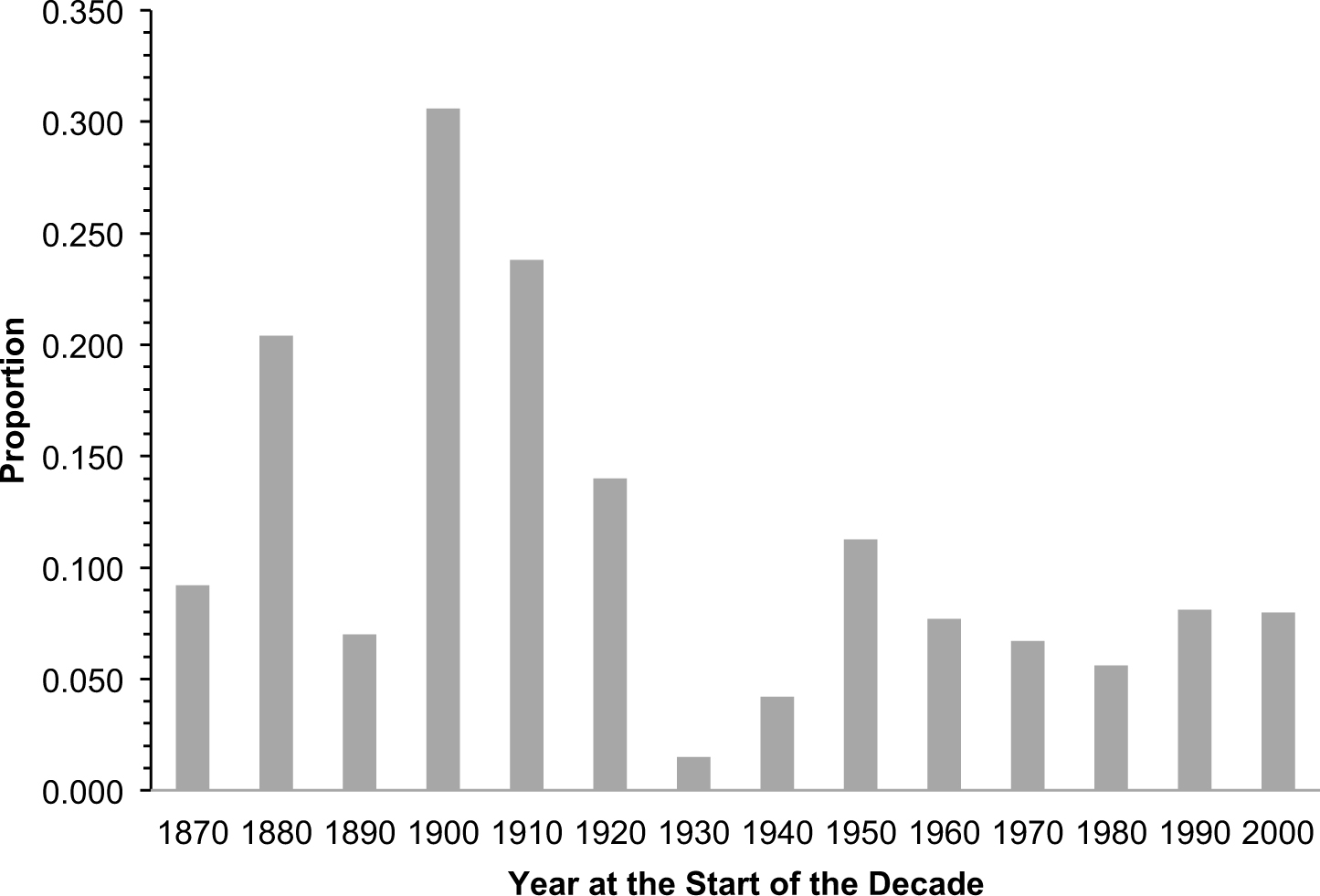
Figure 1 shows the decadal immigration inflows to Canada for each decade since Confederation expressed as a proportion of the start of decade population. The decade from 1911 to 1920 was the second highest inflow decade on record, with the inflow being an astonishing 24 percent of the 1911 population. Because we will be interested in the impact on the earnings distribution in 1920, it is worth noting that nearly two-thirds of that inflow occurred in 1911, 1912, and 1913. But even if we removed those three years, the inflow in the rest of the decade made up 8 percent of the 1911 population, which is the same percentage as for the 2000s. The 1920s inflow was smaller at 14 percent of the start of decade population, but this still makes it the fourth largest inflow on record, and much larger than any decade that has followed. In contrast, the 1930s were the lowest immigration years on record, with the decadal immigration falling to 2.5 percent of the 1931 population.
IMMIGRATION INFLOWS BY DECADE AS A PROPORTION OF START OF DECADE POPULATION
Throughout the early twentieth century, the Canadian labour force and population were defined not only by immigration but also by substantial emigration. In the period from 1911 to 1921, emigration has been estimated at between 78 percent and 85 percent of the gross inflow for the decade (Urquhart and Buckley Reference Urquhart and Kenneth1965, p. 22). Importantly, a large portion of the emigrants were Canadian born or immigrants who had arrived in earlier decades and so it is not necessarily the case that 78 to 85 percent of immigrant arrivals in this decade re-migrated. This is important for us because we are interested in the impact of immigrants on the Canadian earnings distribution and so want to know how many immigrants worked at least a few years in the Canadian labour market. By using Census data on year of arrival, we can obtain the proportion of immigrants who arrived in the years just preceding the Census and who were working in Canada at the time of the Census. Combining that with administrative data on inflows, we find that 37.7 percent of male immigrants who arrived in the ten years before 1921 and 63 percent of those who arrived in the two years before 1921 were in Canada at the time of the 1921 Census.Footnote 5 The fact that a larger proportion of more recent arrivals were still in Canada at the time of the Census indicates that even if many immigrants eventually left Canada, a substantial proportion worked in and potentially had an impact on the Canadian labour market. Indeed, immigrants who arrived in the preceding decade comprised 17 percent of employed males age 15 to 64 in 1921 and 14 percent in 1931.Footnote 6 To take account of emigration related effects, we will work with net changes in numbers of both native born and immigrant workers between Censuses. Thus, our numbers will reflect labour force changes net of emigration and our estimates will include the impacts of the temporary migrants who were in the workforce at the time of the Census but later left.
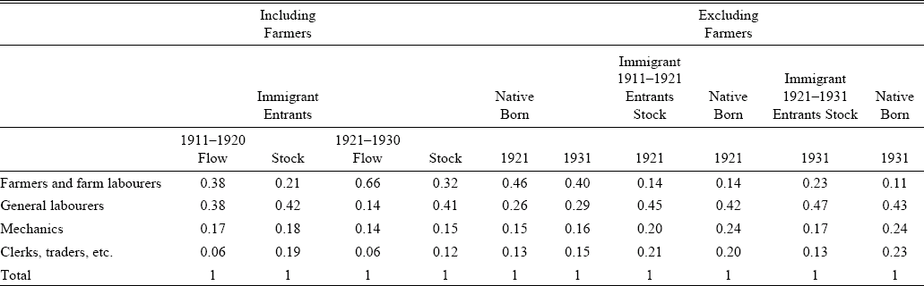
One important question for assessing the impact of immigration on the labour market is whether immigrants actually entered (and stayed) in their intended occupations. Some immigrants would have moved on to the United States, others returned home and still others switched occupations within Canada. To investigate the net impact of these adjustment channels, in Table 1 we present distributions for males across broad occupations from the immigration department flow data and the Census.Footnote 7 Specifically, we sum the number of immigrants entering in each category across the years 1911 to 1920 and then calculate proportions (these are labeled “Flow” in the table). We compare those proportions to the proportions of immigrants in our 1921 Census sample who arrived in the previous ten years (labeled “Stock” in the table). We repeat this exercise for the 1921–1930 period, using the 1931 Census, but do not include numbers for the 1930s because the 1941 Census does not report year of arrival for immigrants. We include occupation distributions for the native born for comparison. Farmers and farm labourers are not separated in the inflow data and in the left panel we also include farmers in the Census data for comparability. The right panel contains Census tabulations of the occupational distributions of immigrants and the native born excluding farmers, which is the sample we will use in our investigations in the remainder of the article.
PROPORTIONS IN BROAD OCCUPATIONS: NATIVE BORN AND IMMIGRANT STOCKS AND FLOWS

Sources:
Flows: Sessional Papers of Canada, various years. Stocks: Census, various years. The left panel includes farmers in the “Farmers and Farm Labourers” numbers to match the inflow data. The right panel is based only on Census data and does not include farmers.
The numbers in the table provide our first main results in terms of understanding the impact of immigrants on the earnings distribution. Immigrants themselves made adjustments that mitigated their potential impact, but did so in different ways in the different policy regimes. The 1910's immigrants had an intended occupational distribution that was similar to the native born distribution in 1921, though more concentrated in the General Labourers category and less in Clerical. By the time we reach the 1921 Census, recent immigrants had moved away from farming occupations and toward both General Labourer and Clerical occupations. Moving to the right panel (which does not include farmers), the result was a recent immigrant distribution that is strikingly similar to that of the native born. The implication is that recent immigrants were much less likely to become farmers than the native born but otherwise were in very similar occupations. That similarity arises both because, under a laissez-faire immigration policy, the migration choices made in the source countries resulted in an inflow that matched the occupational patterns in the host country, and because of adjustments after arrival. The point about choices made before migration is made in Abramitsky et al. (2014), who show that the skill levels of immigrants to the United States in this era also matched well with those of the native born. In Green and Green (Reference Green1993) we examine the intended occupations of a micro sample of immigrants arriving by sea in 1912 and also show that immigrants had a balanced mix of intended occupations that matched both the occupational distribution of the native born and the sectoral growth in the Canadian economy. Based on this and other evidence, we argue in that article that the patterns fit with there being strong informational channels stretching back across the Atlantic.
In the 1920s, Canada's active immigration policy with its emphasis on agricultural labour had an impact that is evident in the stated intentions of immigrants arriving in the 1920s in Table 1. However, among the 1920s arrivals, the percentage in farming declined from the 66 percent who claimed they would enter those occupations when they arrived to the 32 percent who were actually in those occupations in the 1931 Census. As in the 1910s, the distribution shifted away from farming occupations toward the general labourer and clerical categories. But while the Census distribution represents a very substantial shift relative to the inflow, recent immigrants were still quite different from the native born in 1931. In particular, even after dropping farmers, they continued to show a higher share as farm labourers and a lower share in the skilled trades than the native born. This indicates that the more directed policies of the 1920s did have some effect—that it was not simply a case of relabeling immigrants of different types as farmers. Nonetheless, the table shows that in a regime when immigrants were not able to adjust their choices before arrival, they changed occupations to a considerable degree after arrival.
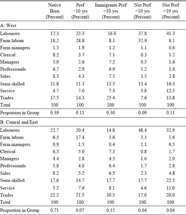
To better understand the nature of the adjustments that immigrants made after arrival, in Table 2, we present more detailed occupational breakdowns from the 1931 Census, with workers categorized as: native born; preferred country immigrants who arrived more than ten years before the Census; preferred immigrants arriving within the last ten years; and non-preferred source country immigrants in both arrival categories. In addition, we show regional breakdowns between the West, and Central and Eastern Canada. Several points emerge from this table. First, the importance of immigration in the West is evident from the fact that 61 percent of the male workforce in that region in 1931 was foreign born. Second, long-standing immigrants from preferred countries were disproportionately represented in the trades and professional occupations and under-represented in both the farm labour and general labourer categories. Third, immigrants from non-preferred countries tended to be heavily represented in the general labourer category and under-represented in more skilled occupations. Fourth, about one-third of the non-preferred country immigrants in the West in 1931 who arrived in the previous decade were in farming, but even for that group a larger proportion were general labourers. Fifth, 71 percent of the non-preferred immigrants who arrived in the 1920s and who were in the West in 1931 were in lower skilled farm or general labour jobs. Sixth, though it is not shown in the table, among the non-preferred group who arrived in the 1920s, 47 percent were in the West. Thus, a large proportion of them ended up in general labourer jobs in the East. This table reinforces the view that immigration policy in the 1920s was effective in the sense that it generated the intended low-skilled labour supply flow to the West. However, it is also evident that this inflow spilled over into other regions and other occupations. Finally, these results imply that in our examination of immigration impacts later in the article, we will need to be concerned about endogeneity since the observed occupational distribution, even of the recent migrants, is clearly not just being assigned to specific regions and occupations through policy.
OCCUPATION DISTRIBUTIONS AT CENSUS DATES BY REGION, 1931

Sources:
Census, various years.
Movements in Earnings Inequality
We now turn to characterizing the shifts in the earnings structure that took place over our sample period (1911 to 1941). This represents the first complete characterization of shifts in the Canadian earnings structure for this period and has been made possible by the recent availability of micro samples from the Canadian Censuses.
DATA AND BASIC PATTERNS
We use microdata samples drawn from the 1911, 1921, 1931, and 1941 Canadian Censuses under the auspices of the Canadian Century Research Initiative (CCRI).Footnote 8 The samples correspond to 5 percent, 4 percent, 3 percent, and 3 percent of the Census population files for the 1911, 1921, 1931, and 1941 Censuses, respectively. The samples are random samples of dwellings with fewer than 30 inhabitants with a more complicated sampling scheme for larger dwellings. We use the weights provided in all of our estimation to take account of this scheme.
The key variable for our purposes is annual earnings which refers to wage, salary, commission, or piece rate earnings from all jobs.Footnote 9 Importantly, the question about annual earnings is identical across the Censuses in our sample, asking the respondent to report “total earnings in the preceding 12 months.” Using a variable on type of work, we selected only “wage-earners” which, in both the introductions to the 1921 and 1931 Censuses is defined as “a person who works for salary or wages, whether he be the general manager of a bank, railway or manufacturing establishment, or only a day labourer.” This definition excludes the self-employed and unpaid family workers (e.g., farmers' sons). It is worth emphasizing that farmers working on their own farm would not be included in our sample even though they make up a substantial share of the overall workforce.Footnote 10 We do not include them because we are concerned that their income would reflect a combination of the wages we are interested in and returns on their capital.Footnote 11 We restrict our sample to males aged 15 to 64.
We convert earnings into 1913 Toronto equivalent dollars using the cost of living indexes in Herbert J. C. Emery and Clint Levitt (Reference Emery and Levitt2002). Because our earnings data correspond to 12-month periods spanning half of two consecutive calendar years, we use the average of the listed 1910 and 1911 values for the first Census, and similar averages for the other Censuses. We use the direct numbers for the 13 larger cities investigated in Emery and Levitt (Reference Emery and Levitt2002) and use the value for the smallest of their cities in a province for workers in smaller towns and rural areas in the province.
Occupation is another important variable in our investigation. The CCRI mapped from Census responses into a joint occupation and industry coding corresponding to the Integrated Public Use Microdata Series (IPUMS) system based on the 1950 U.S. Census codes. We used those codes to form aggregate occupation groups at approximately the three-digit Standard Occupational Classification group level. We drop occupation categories with fewer than five observations in any of our Census samples. The result is 146 consistently defined occupations, which we call the “narrow” occupational grouping. At times, we will also work with a “broad” grouping in which we aggregate the narrow occupations into ten groups: general labourers, farm labourers, farm managers, clerical workers, managers, professionals, sales occupation workers, service workers, semi-skilled workers, and tradesmen.
Finally, we group individuals into five age categories: 15 to 24; 25 to 34; 35 to 44; 45 to 54; and 55 to 64. In our estimations, we work with data aggregated to the age by occupation level since we do not have any observable characteristics within these groups. In those exercises, we make a further cut, dropping all age by occupation cells with fewer than ten observations in any year.
CHANGES IN EARNINGS AND WAGE DISTRIBUTIONS
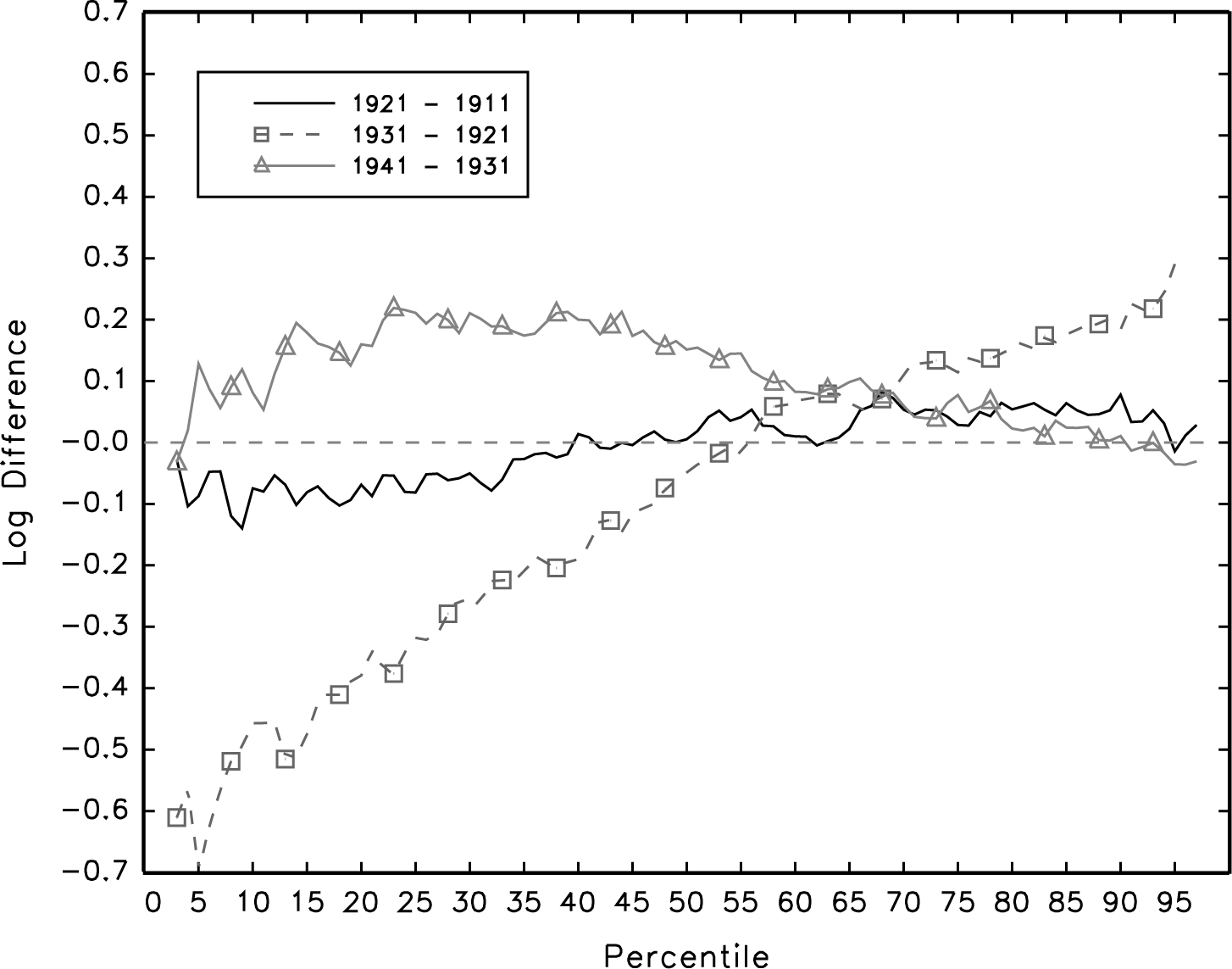
Figure 2 depicts changes in the real annual earnings distribution for each of our three decades (1911–1921, 1921–1931, 1931–1941). The solid line in this figure corresponds to the difference between log earnings in 1921 and log earnings in 1911 at each percentile, and thus roughly shows the proportion differences in the distributions at each percentile. The line with squares shows the same difference between 1931 and 1921, and the line with triangles shows the difference between 1941 and 1931. Importantly, we are comparing percentiles, not specific people, across years; thus, when we report that, say, the 10th percentile declined by 15 percent this does not necessarily mean that a person who was at the 10th percentile in 1911 experienced a decline of 15 percent in his earnings. As a result, the movements depicted in this figure reflect a combination of shifts in real wages within occupations, related changes in rankings of occupations, and changes in the proportion of workers in each occupation. A rising line reflects an increase in inequality between the pair of years as that arises when increases at the top of the distribution are greater than at the bottom.
DECADAL DIFFERENCES IN LOG PERCENTILES: MALE EARNINGS
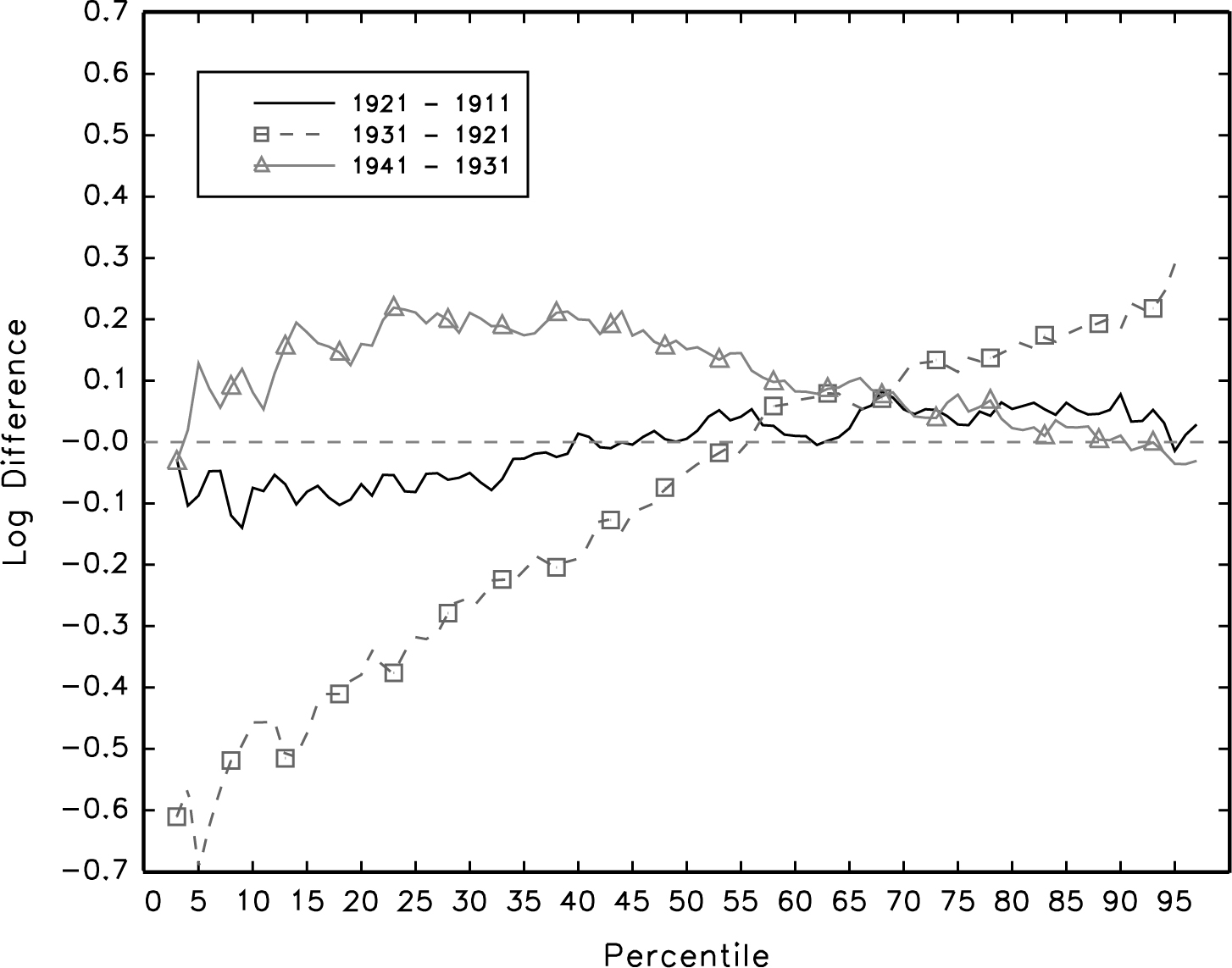
Looking at 1911 to 1921, there is slight evidence of an increase in inequality as the percentiles below about the 30th percentile decline by close to 10 percent in real terms while those in the upper end of the distribution increase by just under 10 percent. These movements, however, are dwarfed by the increase in inequality in the 1920s. Below about the 60th percentile, the real difference line increases linearly from a difference of approximately 0.6 log points (or, about a 45 percent decline) near the 5th percentile to approximately zero near the 55th percentile. Above the 60th percentile, the differential continues to increase across percentiles, though at a slower rate. The ratio of the 95th to the 5th percentiles rises by a factor of almost 10 in this decade. Finally, over the 1930s there is a decrease in inequality as the top of the distribution changes very little compared to approximately 20 percent increases through much of the lower half of the distribution. In spite of this, the net effect over the whole period from 1911 to 1941 is a strong increase in earnings inequality. Overall, the figure indicates that Canada underwent a substantial long-term change in its earnings structure between 1911 and 1941. Roughly speaking, this can be broken down into: a decade with small inequality increases from 1911 to 1921; a decade with a very substantial increase in inequality, driven particularly by large real earnings declines at the bottom of the distribution, from 1921 to 1931; and a mixed period with some reductions in inequality from 1931 to 1941.
The other two main investigations of wage movements in this era are Emery and Levitt (Reference Emery and Levitt2002)'s study using data from the Labour Gazette and Mary Mackinnon (Reference Mackinnon1996)'s work using data from the Canadian Pacific Railway (CPR). Emery and Levitt (Reference Emery and Levitt2002) focus on regional wage differentials and do not directly discuss movements in national inequality, while Mackinnon (Reference Mackinnon1996) provides some discussion of wage differentials between skilled trades and labourers. We provide a detailed comparison of results from Census data with the results from both of these other articles in the Online Appendix. Our main conclusion is that the Census data accords well with the Labour Gazette data in terms of long term movements in labourers' wages and wage differentials between the skilled trades and labourers but less well with Mackinnon's CPR data. Given coverage issues with both the CPR and Labour Gazette data, we view the Census data as the most reliable, but we are reassured by the matching of broad patterns between it and the Labour Gazette data.
Regardless of these specific comparisons, it is important to note that all earlier work on wage inequality for Canada has been done in terms of ratios between specific occupations—most often between skilled, blue collar trades or clerks and labourers. Ours is the first presentation of which we are aware of the entire earnings distributions for these years. In our data, general labourers have earnings that place them at approximately the 25th percentile of the overall earnings distribution and the skilled trades and clerical workers have earnings near the 75th percentile. Using the Census micro data, we are able to see whether movements in the skill differential (i.e., what is essentially the 75–25 ratio) are indicative of the overall changes in inequality. An examination of Figure 2 indicates that given the relative similarity of changes in earnings above about the 60th percentile, following the 75th percentile does a good job of capturing movements in the upper tail of the distribution. But the lower tail of the distribution shows a much stronger decline than that observed at the 25th percentile in the 1920s and smaller increases in the 1940s. Thus, focusing on skilled worker versus labourer wage differentials leads to a substantial understatement of the extent of the increase in inequality in earnings over this period.
Decomposing the Changes in the Earnings Distribution
We turn now to the question of whether the changes in earnings inequality in this period are linked to the immigrant inflow. The most direct way for the immigrant inflow to affect the earnings distribution is through shifting the composition of the workforce. In the absence of general equilibrium impacts on wages, an immigrant inflow concentrated, for example, in low-skilled occupations would imply a fattening of the left tail of the earnings distribution. In this section, we decompose the decadal changes in Canada's earnings distribution into factors related to immigrant status, age, and occupation.
A change in the earnings distribution can arise through three channels: changes in the distribution of workers across skill related categories (immigrant status, age, and occupation, in our case); changes in the differences in average earnings between those categories; and changes in the dispersion of earnings within the categories. We have already discussed the occupational component of the first channel for immigrants. Table 1 also indicates that the native born occupational composition was relatively constant over this period.
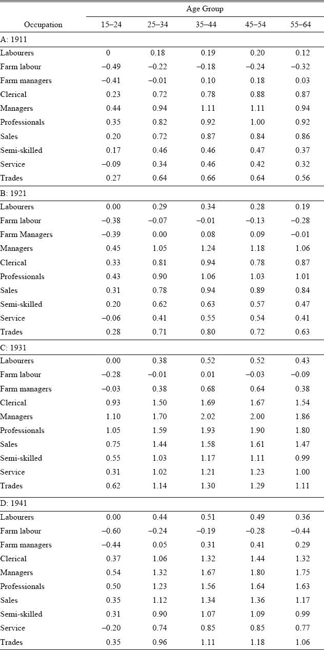
To investigate the between group wage differentials, in Table 3 we present differences in average log wages between groups defined by ten occupation groups and five ten-year wide age groups and the average log wage for a base group (15 to 24 year old general labourers) for each Census year. The wage differentials in 1911 and 1921 were quite similar. In both cases, there were substantial increases in wages between the 15–24 year olds and the 25–34 years olds for all occupations. But age differentials beyond age 24–34 were quite flat, even for white-collar occupations like professionals. Virtually all occupations also showed a small decline in average earnings between ages 45–54 and 55–64. The cross-occupation differences at a particular age line up with expectations, with the highest wages for managers and professionals, the lowest for labourers, and semi-skilled and skilled white and blue-collar workers falling in between.
DIFFERENCES IN AVERAGE LOG WAGES BY AGE AND OCCUPATION

Sources:
Census, various years. The table entries for each year show the difference in average log wages between each occupation by age category and the average log wage for general labourers aged 15 to 24 in that year.
Between 1921 and 1931, the earnings structure changed in two ways. First, we see the emergence of more substantial age differentials. For example, the difference between 25–34 year old and 35–44 year old managers was 0.19 log points in 1921 but 0.32 log points in 1931. Second, the earnings differentials among blue-collar occupations and between white-collar and blue-collar occupations increased substantially, particularly. As an example, the earnings differentials between trades occupations and semi-skilled workers and labourers were 0.07 and 0.46 log points, respectively, in 1921. These rose to 0.13 and 0.78 in 1931. In contrast, the differential between clerical workers and managers was virtually unchanged over this period. Finally, between 1931 and 1941, the age differentials either stayed the same or increased slightly while the occupation differentials tended to decrease.
To obtain a measure of changes in within occupation earnings dispersion, we estimated the difference between the 90th and 10th percentiles of the log earnings distribution for each of our ten broad occupation categories, holding the age dimension constant by looking only at 35–44 year olds. The average of these 90–10 differentials across occupations took values of 1.22 in 1911, 1.23 in 1921, 1.65 in 1931, and 1.63 in 1941. Overall, the earnings calculations indicate that the wage structure (both between and within occupations) changed substantially between 1921 and 1931 but moved only mildly in the decades before and after that.
To judge the relative importance of the composition shifts versus the changes in the wage structure, we employ the ingenious decomposition technique developed in Sergio Firpo, Nicole M. Fortin, and Thomas Lemieux (2009) (hereafter, FFL). At the core of the FFL methodology are influence functions, which show the influence of an observation on the value of a given statistic. Of particular interest is their demonstration that once the influence functions for quantiles are “recentered” around the sample quantile values, one can decompose movements in the quantiles of a distribution in a manner directly analogous an Oaxaca decomposition. In particular, one can assess the extent to which shifts in the distribution of observable characteristics shift specific quantiles. We use their methodology to assess the impact of shifts in four personal characteristics on the earnings distribution: age (arranged in five, ten-year groups); occupation (in the 146 groups described earlier); whether a person was a recent immigrant (an immigrant who arrived in the ten years prior to the Census); and whether a person was an established immigrant (an immigrant who arrived more than ten years before the Census). Native born workers form the omitted category.Footnote 12
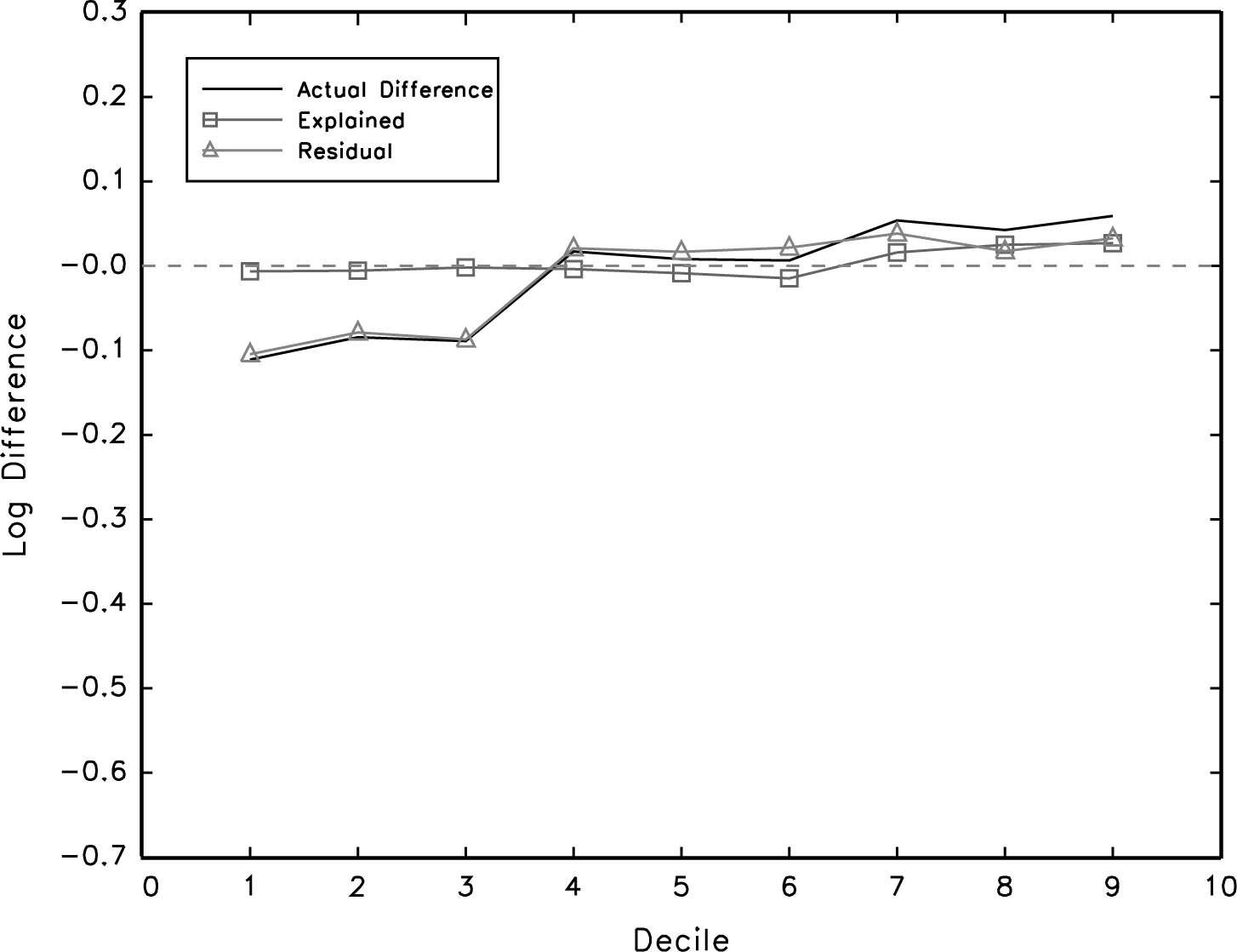
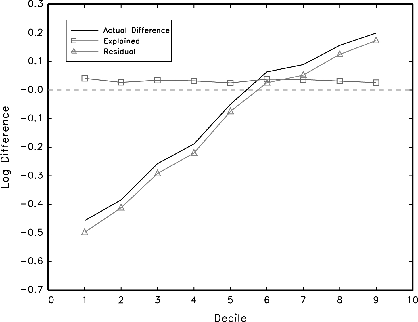
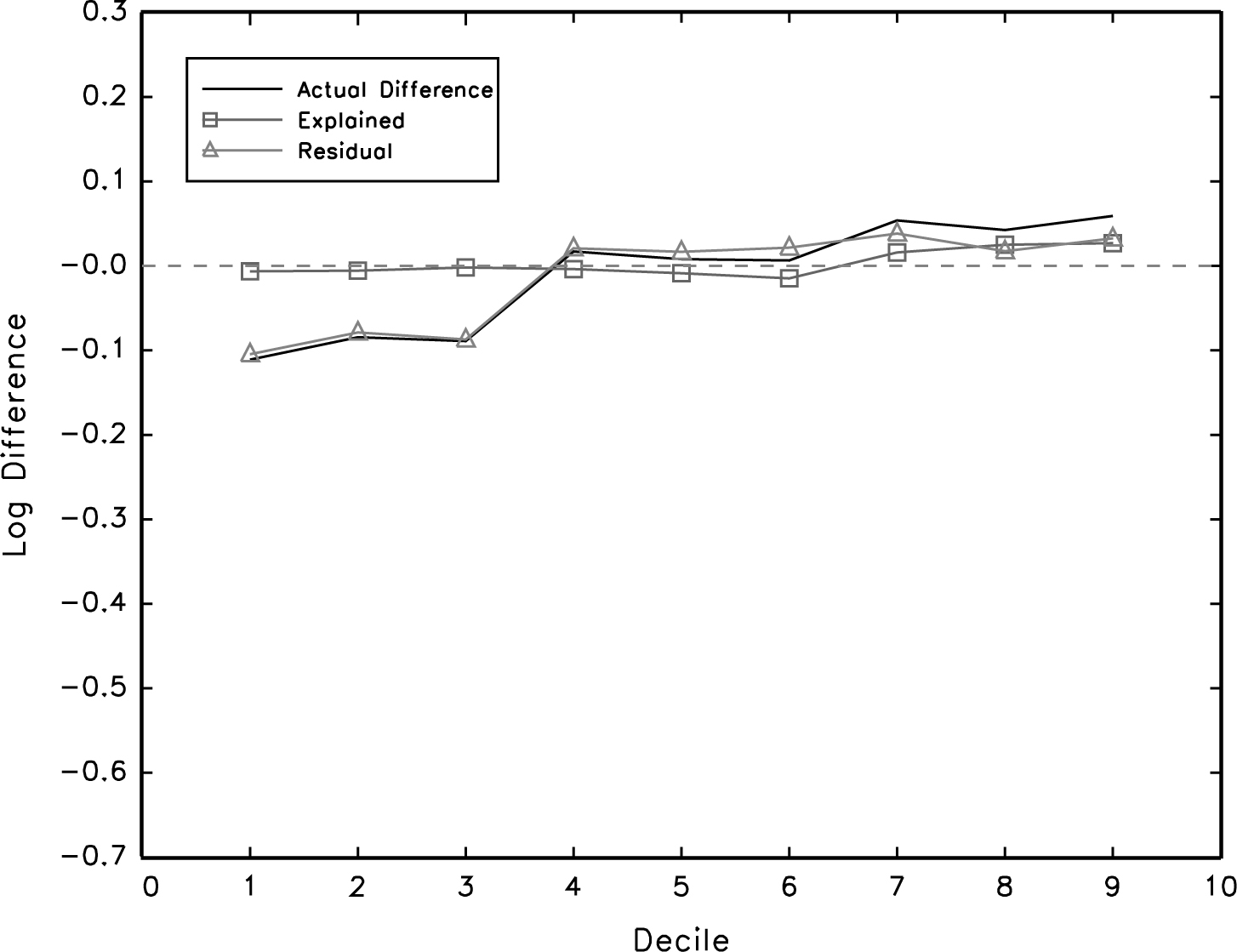
In Figure 3a, (in the line labeled “actual difference”) we plot the change in each decile of the real earnings distribution between 1911 and 1921. This is a re-plotting of the relevant line in Figure 2 but only showing the decile points. The line labeled “Explained” shows changes in a given decile due to changes in the composition of the labour force along the age, occupation, and immigration dimensions. The third line (labeled, “Residual”) equals the difference between the actual change and the change arising purely from changes in the composition in terms of observables. It corresponds to the change that would have happened if the composition were held constant. As such, it captures the impact of changes in the quantile specific coefficients associated with the observables (including the intercept) and reflects changes in returns to observable and unobservable worker characteristics. For the 1911–1921 period, shifts in observable characteristics, including immigrant status, explain very little of the overall change in earnings inequality below the 7th decile. However, those composition shifts play an important role at the top of the distribution, explaining 30 percent, 60 percent, and 45 percent of the movements at the 7th, 8th, and 9th deciles, respectively. For the 1921–1931 changes shown in Figure 3b, composition explains a similarly small proportion of changes in the lower two-thirds of the distribution. In the right tail, composition again explains more but to a lesser extent than in the previous decade (explaining 40 percent, 20 percent, and 13 percent of the top three deciles in ascending order).
FFL DECOMPOSITION, 1911–1921
FFL DECOMPOSITION, 1921–1931
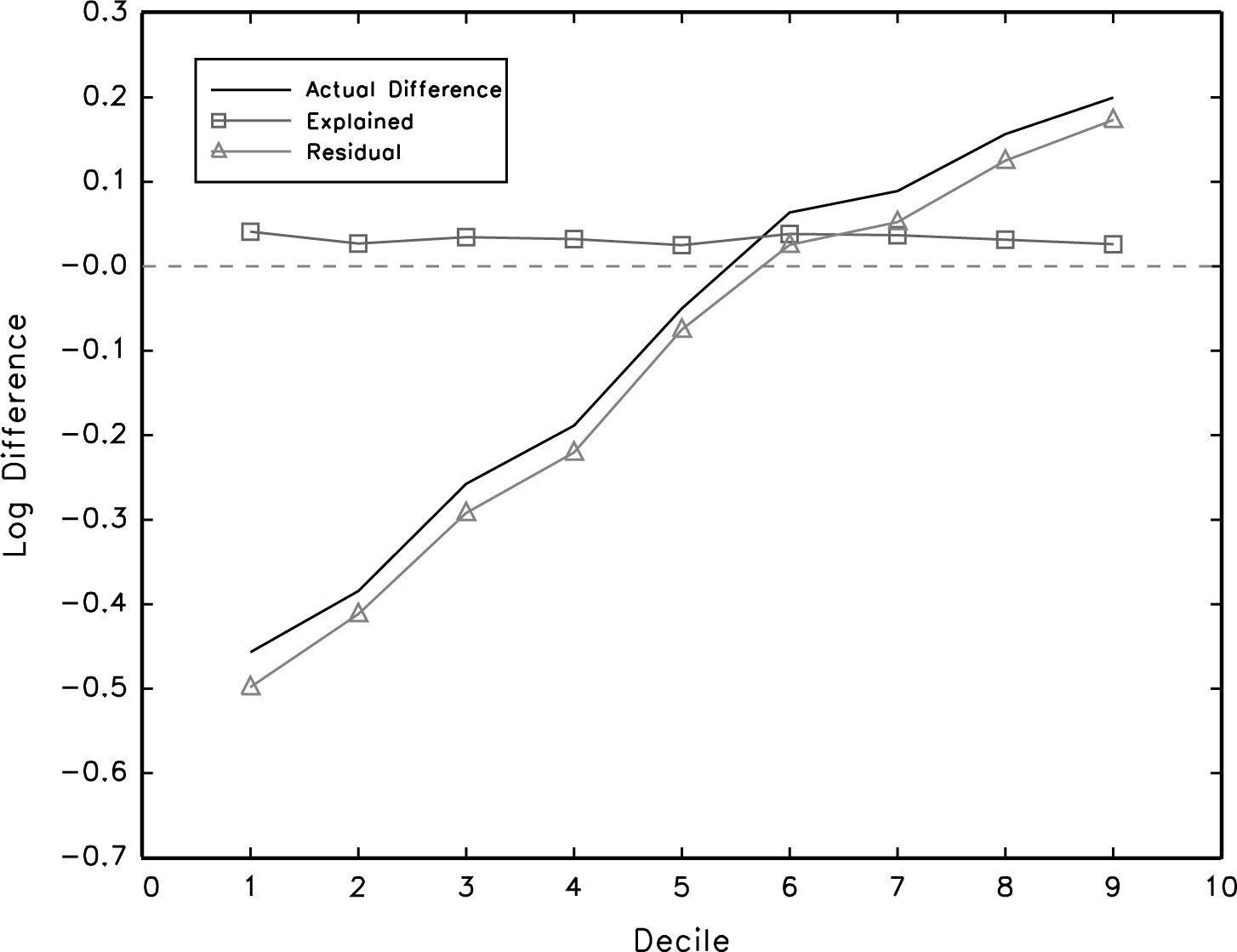
The overall conclusion from the decomposition exercise is that movements in observable characteristics, including changes related to the inflow of immigrants, were not a major determinant of movements in the real earnings distribution. Most importantly, they explain little of the substantial decline in the lower tail of the real earnings distribution in the 1920s. That decline arises from a combination of the increased earnings differentials between age-occupation groups and the increase in within-group dispersion. In a counterfactual exercise for the 1921–1931 decade reported in the Online Appendix, we generate the change in the earnings distribution that would have arisen if there had been no within-group variation. Based on that exercise, within group variation plays a varying but generally important role in inequality changes below the median but essentially no role above the median.
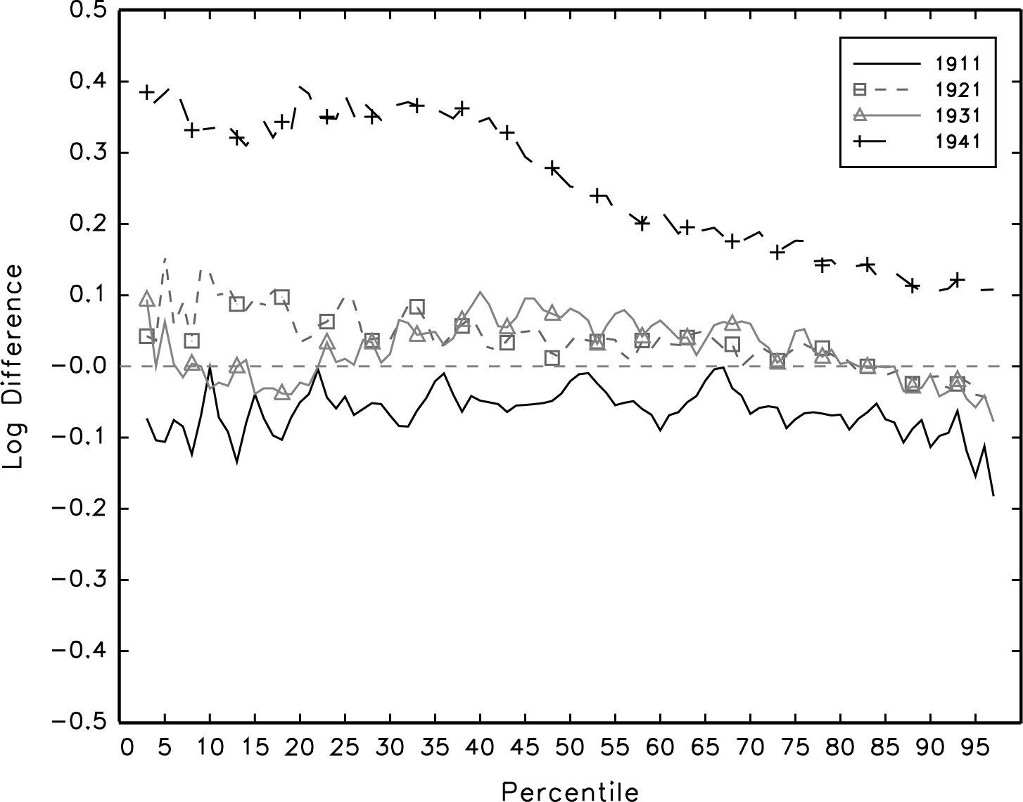
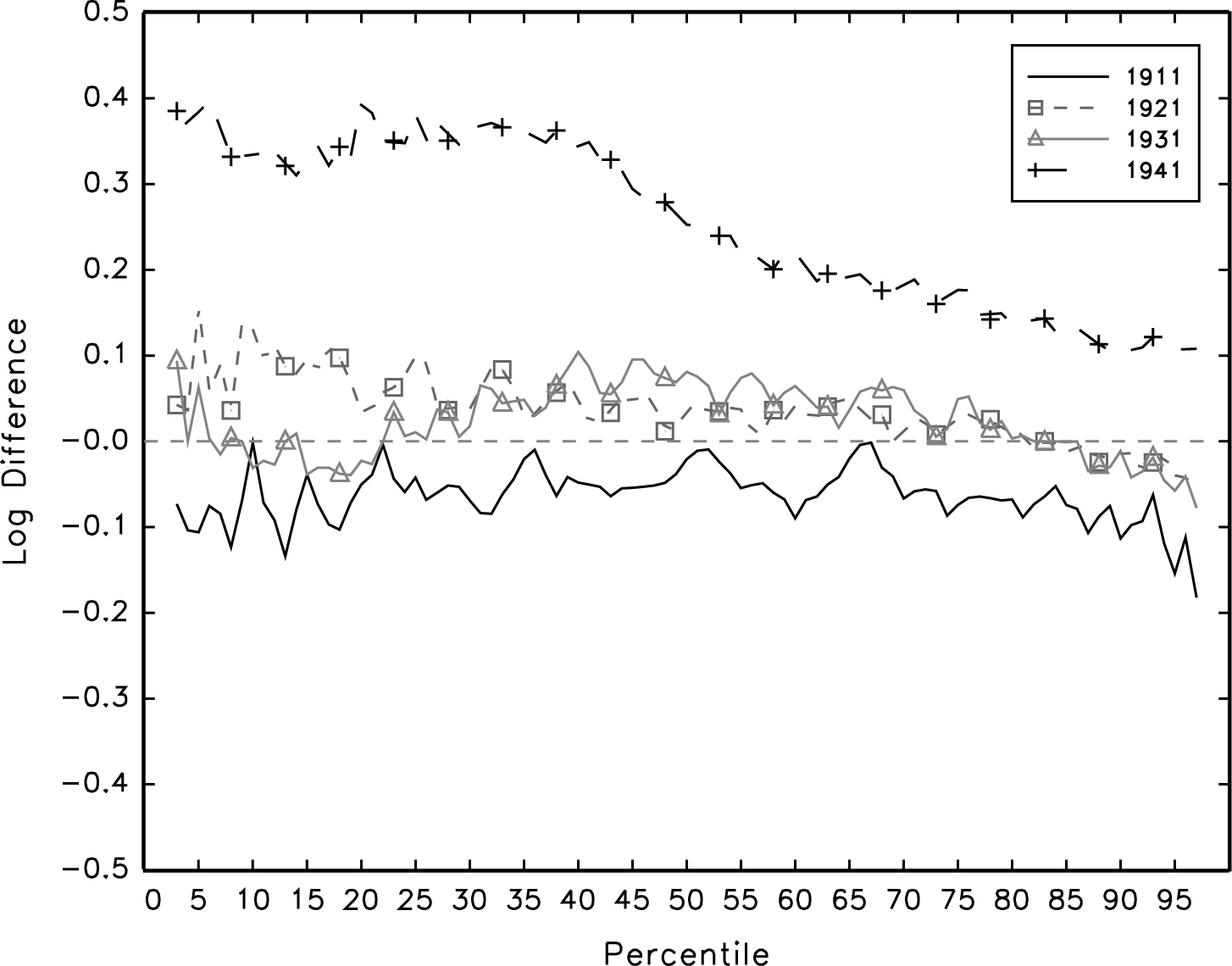
To better understand the role of immigration in these decompositions, in Figure 4 we plot differences in percentiles of the immigrant and native born earnings distribution for each Census (immigrant minus native born). The striking point from the figure is that for the 1911, 1921, and 1931 Census years, the immigrant and native born earnings distributions were very similar, with differences typically below 10 percentage points. For 1941, the immigrant earnings distribution is strongly superior to that of the native born. However, since there had been virtually no immigration for a decade, the immigrant workforce was older than the native born in 1941 and this difference likely just reflects returns to experience rather than a true immigrant advantage. Given that immigrant and native born occupational distributions were broadly similar, the similarity of the earnings distributions implies that there was not systematic discrimination (or differentials in productivity) between immigrant and native born workers.Footnote 13 It also explains why the decomposition exercise shows little effect from the immigration inflow. However, this is not the final answer on whether the immigration inflow affected the wage structure since this decomposition exercise ignores general equilibrium effects in the form of the immigration inflows altering occupation specific wages over time. To assess the latter potential impacts we will need to use a structural model of wage determination, and we turn to that in the next section.
IMMIGRANT MINUS NATIVE BORN DIFFERENCES IN LOG PERCENTILES: MALE EARNINGS
ESTIMATING THE IMPACT OF IMMIGRATION ON CHANGES IN THE WAGE STRUCTURE
In this section, we examine whether immigration affected earnings inequality in inter-war Canada using techniques from recent papers on the impact of immigration on the native born wage distribution. Given the evidence in the section on immigration policy patterns showing potentially endogenous geographic adjustments by immigrants after arrival, we follow approaches that focus on national level wage and employment patterns as opposed to approaches comparing local labour markets.
NESTED CES MODEL
We address the impact of immigration on the wage structure using a quasi-structural estimation approach based on a nested CES production function. Our specification closely follows Gianmarco I. P. Ottaviano and Giovanni Peri (Reference Ottaviano and Peri2012) (hereafter, OP) and Francesco D'Amuri, Ottaviano, and Peri (Reference D'Amuri, Ottaviano and Peri2010) (hereafter, DOP). This approach allows for a complete accounting of the impacts of immigration by incorporating the potential effects of an increase in the supply of immigrants in one occupation on the wages for other workers through substitutabilities and complementarities in production. Of course, the CES specification, even in its nested form, imposes significant restrictions on allowable patterns of interactions of use of factors that should be kept in mind. The Online Appendix contains a more detailed account of the estimation approach. Alternatively, readers not interested in estimation and identification issues can skip ahead to the exercises in the Counterfactual Exercises section.
We begin by considering the aggregate production specified as a simple Cobb-Douglas function of a labour aggregate, Lt , and capital, Ct :

where Yt is aggregate output and At is a productivity shifter.Footnote 14 We will assume that the economy faces fixed world prices for the output but that Ct is less than perfectly elastically supplied (perhaps because it includes scarce factors such as land in the rural sector, and entrepreneurial ability in the other sectors). This implies downward sloping labour demand curves.Footnote 15
Following DOP, we specify the labour aggregate as a CES function of types of skilled labour defined by our ten broad occupation groups. Given this specification, the labour aggregate in period t can be written as:

where Lkt is employment in occupation k, and θkt are skill-time specific productivity shocks. The parameter σ determines the degree of substitutability among broad occupation groups.
We capture further worker dimensions through a sequence of nestings. First, we treat labour in each broad occupation group as a CES aggregate of employment of the narrow occupations that fit in the broad group. The employment in the narrow occupations is, in turn, a CES aggregate of workers in the five age groups. Within age groups, we divide workers between recent immigrants and a combination of established immigrants and the native born. We implement this division because of the similarity of the established immigrant and native born occupational distribution. The final level of nesting contains the native born and established immigrants separately.
Using the nesting specifications, and again following DOP closely, we can derive a wage equation for a native born worker in broad occupation k, narrow occupation l, and age group j assuming their wage equals their marginal product:

where, L's correspond to employment levels for groups defined by occupation and age, ENkljt is the number of combined established immigrants and native born workers in the cell defined by occupation and age, Nkljt is the number of native born workers in that cell, and θ's correspond to productivity shifters. The parameters σo , ρ, δ, and φ determine, respectively, the degree of substitutability among narrow occupations, age groups, between recent immigrants and all other workers, and between established immigrants and the native born. We can similarly derive the log wage equations for an established immigrant worker in the same cell.
As OP point out, inspection of equation (3) reveals several channels through which an immigrant shock in a specific occupation by age cell can affect the wage of any native born worker. First, the fact that labour of different types is imperfectly substitutable implies that all workers benefit from an increase in the total number of workers in the economy. This is captured in the second term on the right hand side of equation (3), which is positive. The fourth term on the right hand side captures the effect of increased immigration within the same broad immigration group. This effect will be negative if the elastisticity of substitution among broad groups is less than that among the narrow groups within broad groups (as seems likely). This, and the overall size effect captured in the second right hand side term, are the channels through which immigration in the same broad occupation group but a different narrow occupation group can affect a worker's wage. Similarly, the sixth term allows us to capture the effects of immigration in the same narrow occupation but different age group and the eighth term reflects the direct effect of immigrants entering in the same narrow occupation and age group. The last two quantity terms in the expression relate to previous arrivals and the native born and so will not change with immigration (Ottaviano and Peri Reference Ottaviano and Peri2012).
Estimating Equations and Results
The parameters in the nested CES model can be obtained sequentially, moving up the levels of aggregation. Thus, following OP, we can obtain an estimate of φ by taking the difference between the log wage expressions for native born and established immigrant workers:

where, Ekljt is the number of established immigrants in the occupation by age cell, wEkljt is their average wage, and θEkljt is the productivity shifter associated with those immigrants. This yields an intuitive formulation: holding constant relative differences in productivity (the θ's), comparing relative differences across cells in wages and employment levels between established immigrant and native born workers tells us about the substitutability of the two types of workers. If we see a large relative jump in established immigrant employment but comparatively small changes in their relative wages, for example, we would conclude that established immigrant and native born workers are very substitutable in production—that the established immigration increase affected immigrant and native born wages similarly. Defining cells as narrowly as possible makes it more plausible that there are no productivity differences between the worker types. Thus, established immigrant and native born agricultural labourers of the same age would reasonably be expected to be working with the same technologies and thus to have the same θ's. To isolate this cell-level variation, we include separate occupation, age, and time effects. This is equivalent to assuming that we can write,

where the ψ's are fixed effects and ukjt is an independent error term. Identification then relies on the assumption that relative supplies of native born versus established immigrants may respond to longer run factors such as the persistent occupation, age, and time effects captured in the included fixed effects, but do not respond to the idiosyncratic disturbances to productivity reflected in ukjt .
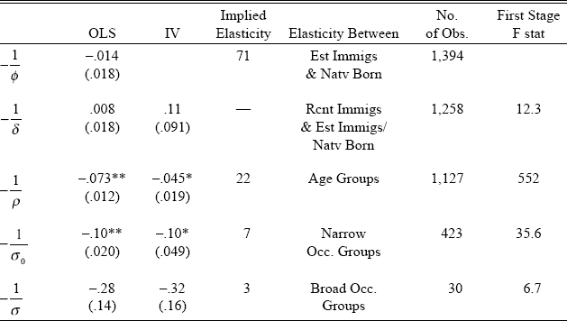
We run equation (5) using real annual earnings and employment numbers from the Census data aggregated to the narrow occupation group level. We weight using the square root of the cell size. The dropping of small or empty cells leaves 1,534 occupation by age group cells. Standard errors are clustered at the occupation × age group level to allow for flexible forms of serial correlation in the error term. When we move to working with recent immigrants in the higher nesting levels, we will create instruments to address potential endogenous adjustments by the immigrants, but no such instrument is available for the older immigrants and so we only present ordinary least square (OLS) results for this regression. In Table 4, we present the key estimated coefficients (the negative inverse elasticities) and the implied elasticities from each stage of the CES nesting.
NEGATIVE INVERSE ELASTICITIES OF SUBSTITUTION FROM CES ESTIMATION

Sources:
* + Significant at the 5 percent level.
** + Significant at the 1 percent level.
Notes:
The calculated elasticity is based in the IV estimate in all rows except for the elasticity between established immigrants and the native born, where there is no valid instrument.
Specifications for the first two rows include year, age, and occupation fixed effects. The remaining rows include year and occupation fixed effects.
Standard errors in parentheses. Standard errors are clustered at the occupation by age group level in the first three rows, and at the occupation levels in the remaining rows.
Source:
Authors' calculations based on data from Census, various years.
Our estimate of the negative inverse elasticity of substitution is −0.014 and not statistically significant at any conventional level. This falls in the lower part of the range of estimates from DOP for modern day Germany and OP for modern day United States (–0.01 to −0.06). The corresponding elasticity from our estimates is 71, implying that established immigrants and native born workers are almost perfectly substitutable in production, as we predicted.
We next move one step up in the nesting hierarchy to consider substitutability between workers already in Canada (both native born workers and established immigrants) and recent immigrants within the same age-occupation cell. To do this, we aggregate equation (3) to the established/recent immigrant worker level to obtain a wage expression for the combined native born/established immigrant group. We obtain an expression for the wage for a recent immigrant in the same way and then take the difference between the two wage equations to obtain:

where, wIkljt
is the average wage for recent immigrants, θIkljt
is the productivity shifter for recent immigrants, Ikljt
is the number of recent immigrant workers, and  is the weighted average of established immigrant and native born wages in the occupation-age cell, with the weights being the proportions of established immigrant and native born workers. We again assume that the ratio of productivity terms can be captured by occupation, age, and time fixed effects plus an idiosyncratic error term.
There is reason for concern about the endogeneity of the immigration supply changes even after including the fixed effects. In particular, we know that immigrants who were explicitly brought in to work in agriculture in the West, were, by the time we observe them in the next Census, in a variety of occupations and locations. Thus, the set of changes in immigrant employment we observe might partly be due to endogenous responses to within-cell productivity shocks. We use a variant of an instrument originating with David Card (Reference Card2001) in which we assume that immigrants move to a geographical location based partly on joining an enclave of people from their country of origin and then, once there, pursue the most common occupations in that location. That is, we assume that when they search for a job in the location they are attracted to for companionship reasons, their probability of finding a job in a given occupation is proportional to the size of that occupation in that location. Moving to a mining town, immigrants are more likely to find mining jobs than if they moved to Toronto.
To construct the instrument, consider an immigrant from source country g, and let the proportion of immigrants from g in location r in year t be given by pgrt . Also, let the proportion of all workers in narrow occupation l that is within broad occupation k in location r in period t be given by πklrt . We will predict the number of people from country g in occupation k in year t+1 at the national level as:

where n10gt
+1 is the number of immigrants from country g who arrived in the previous 10 years at the national level. We do this exercise separately by age group with both the πklrt
weights and the national level inflows (ngt
+1) being age group specific.Footnote
16
Finally, we form our instrument for  as
 . The first stage F-stat for this instrument is 12.3, implying that we do not have a weak instrument problem.
The key identifying assumption is that neither the composition of employment by occupation at the start of a period in a location nor the distribution of immigrants from a given country across locations at the start of the period are correlated with the change in productivity within an occupation-age cell at the national level in the ensuing decade. We also require that the general growth in immigration from each country is not correlated with the cell specific productivity shocks. These assumptions would be violated if people from a given source country only immigrated to Canada because there was an increase in demand for a specific occupation in a specific location. For example, if all migrants from Lithuania were miners and they all went to Northern Ontario because there was an ongoing increase in demand for miners across decades in that region, the instrument would be problematic. In that case, the correlation between past concentrations and recent inflows of Lithuanians to the region would partly reflect productivity trends rather than just living situation preferences. The fact that πkrt
is calculated for all workers in the location, not just for immigrants from the specific source country, makes it more likely that the requirements for the instrument to be valid are met. Both the OLS and Instrumental Variables (IV) estimates of  are positive and insignificant. We interpret this as implying that recent immigrants and previously arrived workers are perfect substitutes.
Next, we aggregate the wage equations to the occupation-age level. We can write an expression for  , the weighted average of immigrant and native born wages in the sector-occupation-age cell, with the weights being the proportions of immigrant and native born workers. If we choose an arbitrary age group, j + 1, as the base group, we can take the difference between the mean wage of any other group and the base group to arrive at:

Because we want to isolate variation within occupation-time cells to make it more likely that the relative θ values can be considered to be equal, we run this regression in differences including full sets of separate occupation, age, and time dummies. This allows for separate trends for each age and occupation group. We instrument for the employment ratio using the log of the ratio of our n10kljt
variable for each age group relative to the base group value for n10kljt
. The resulting first stage is strong (with an F-stat of 552). The omitted category is workers aged 25 to 34 and we drop that group from the estimation. Our IV estimate of  is −0.045 and is statistically significant at the 5 percent level. The implied corresponding elasticity of substitution is 22, which is large but considerably below the substitutability among immigrant and native born workers within age by occupation cells.
Aggregating up to the narrow occupation group level, we arrive at,

where  is the average wage in the occupation cell in period t. If we assume that the first three terms on the right hand side of equation (9) can be captured by occupation and time effects then we can estimate equation (9) including those effects, using within occupation over time variation. As at the third level, we run the regression in differences and include occupation and time dummies. We instrument for the change in ln Lklt
using the log of the n10kljt
variable aggregated up to the narrow occupation level. The first stage F statistic is again large at 35.6. The resulting estimate of
 is −.10 and is statistically significant at the 5 percent level. The implied elasticity of substitution among narrowly defined occupations within a broad occupation group is 7.
Finally, we aggregate up to the broad occupation group level and estimate the analogous equation to equation (9) using the same methods. Again, the instrument is based on an aggregated version of n10kljt
. The IV estimate for  is −0.32, which is not statistically significant at the 5 percent level. In this case, we do have a weak instrument problem, with a first stage F-statistic of 6.7. However, based on the combination of this estimate, the OLS estimate, and other IV estimates reported in the Online Appendix, we are confident that the estimated inverse elasticity is larger than that for the previous stages. In the simulation exercises in the next section, we use the IV point estimate, −0.32, which corresponds to an elasticity of substitution for broad occupation groups of three.
Counterfactual Exercises
The estimated elasticities are of limited intuitive value on their own but can be used with the equation for native born wages, equation (3), to investigate the impact of immigration on native born wages. Our approach to quantifying that impact is to focus on the 1921–1931 decade, constructing counterfactual wage distributions corresponding to: (1) no immigration between 1921 and 1931; and (2) no general or agricultural labourer immigration in that decade.Footnote
17
To construct the first counterfactual, consider generating a fitted wage for 1931 using equation (3) but with the number of recent arrival immigrants subtracted from each relevant labour measure on the right hand side. Importantly, this counterfactual is based on the number of new immigrants observed in the 1931 Census and so already nets out any effect that emigration would have in reducing the impact of initial immigration inflows. Since the productivity terms (the θ's and ln  (Kt
, Lt
)) are assumed not to change with immigration, we can construct the counterfactual wage in 1931 as,

We then construct a complete counterfactual distribution by creating a set of “phantom” people for each occupation by age cell. That is, if a given cell has nklj native born workers in it in 1931 then we generate nklj phantom people all with the fitted wage, wNklj c . Doing this for each cell, we obtain a dataset that has the same size and distribution of workers across cells as the true 1931 data but with fitted wages that reflect the estimated elasticities and the counterfactual quantities.
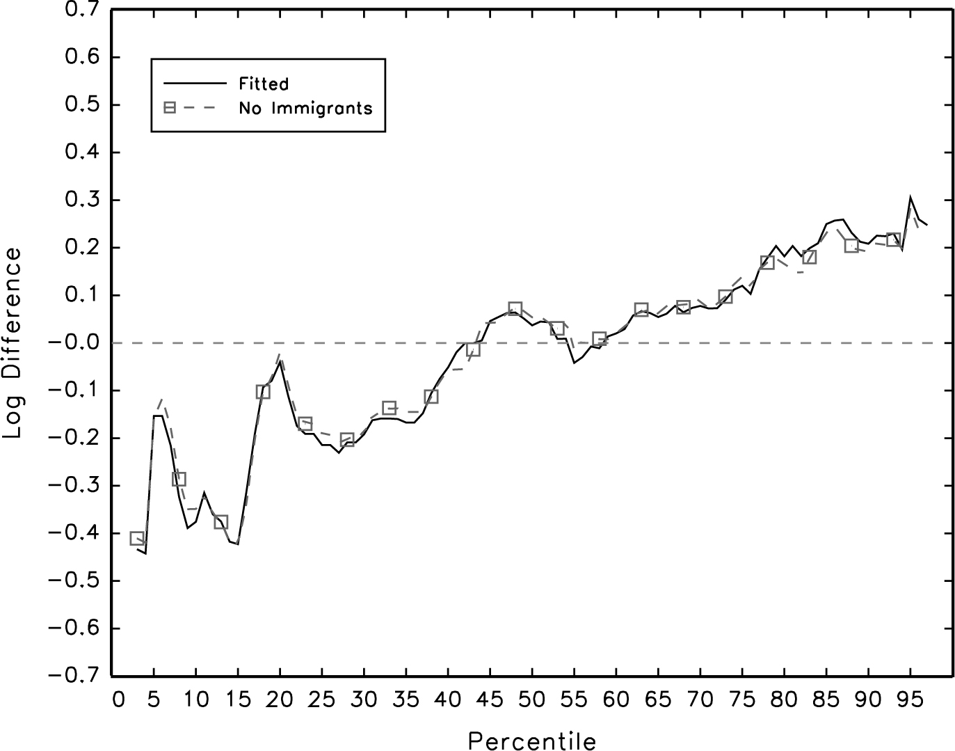
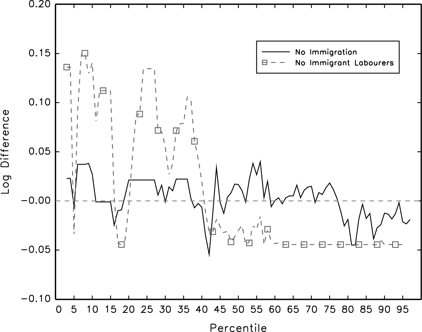
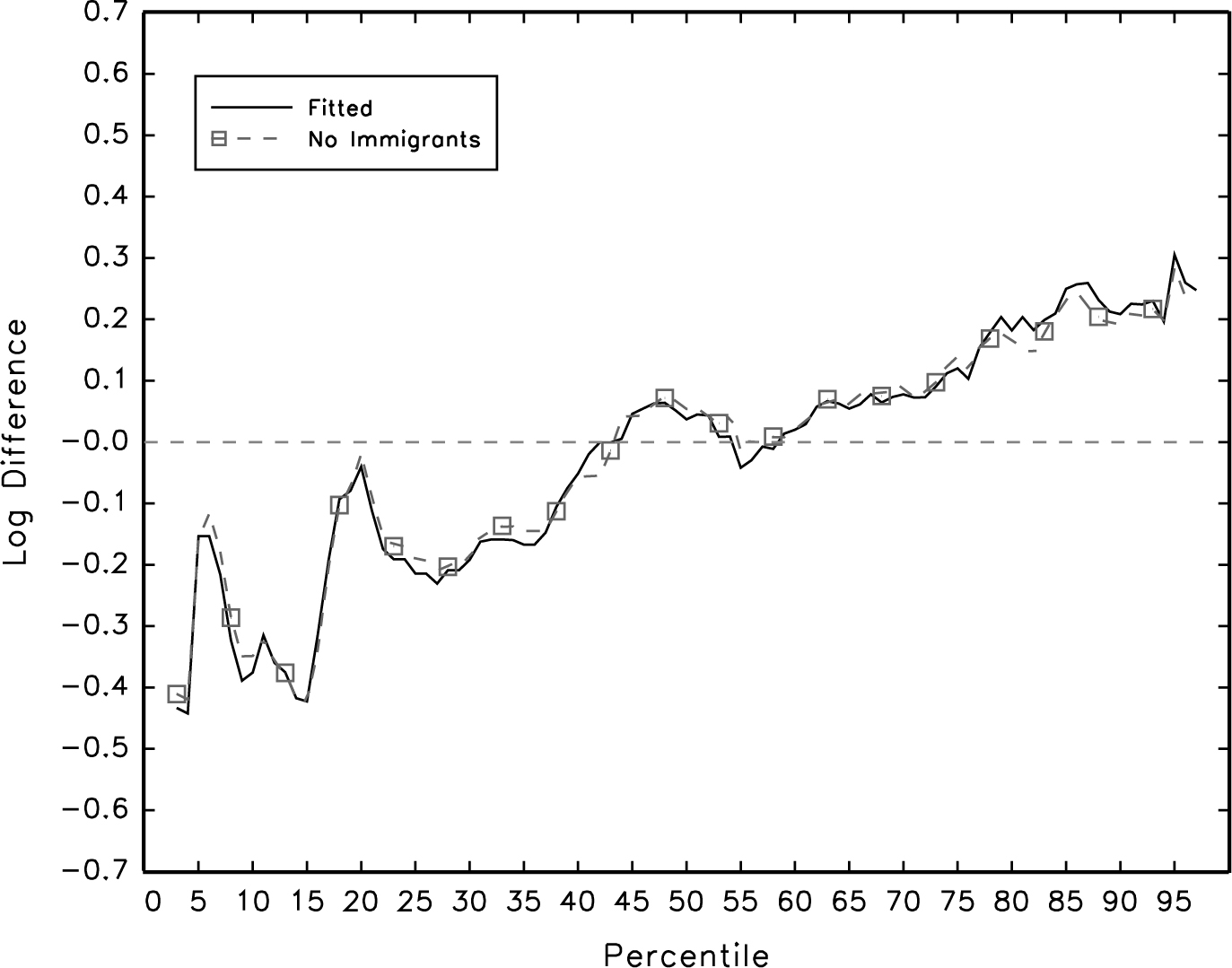
To capture the impact of not having immigration, we need to compare this counterfactual distribution to the actual distribution. This requires forming versions of the true distributions that eliminate within occupation by age cell wage variation, just as the counterfactual exercise does. We do this for both 1921 and 1931 by again constructing a set of phantom workers for each cell but, in this case, assigning them the actual average wage for the relevant cell in the given year. We compare the result to the true change in the distribution in the Online Appendix. We find that removing the within-cell variation does not substantially alter the picture of increased earnings inequality in the 1920s, although the extent of the decline in earnings in the lower tail of the distribution is reduced. In Figure 5a, we plot the difference in log percentiles from these fitted distributions along with the difference between the log percentiles of the 1931 counterfactual distribution with no recent arrival immigrants and the 1921 fitted distribution. The result is a small implied immigration impact across the distribution. This can be seen more clearly in Figure 6, where we plot the difference in log percentiles between the counterfactual distribution and the fitted 1931 distribution. This difference provides our key estimate of the net impact of immigration on the earnings structure in this period. Because the number of immigrants we remove from the 1931 labour force to construct the counterfactual come from the Census, they reflect the adjustments made by immigrants within Canada. Given our earlier arguments that the occupational distribution of recent immigrants is similar to that of the workers already in Canada, taking them away from the distribution implies small changes in the distribution. But the occupational distributions of recent arrivals versus established workers are not identical and the small impact partly reflects general equilibrium adjustments.
FITTED AND COUNTERFACTUAL DIFFERENCES WITH NO IMMIGRATION: MALE EARNINGS, 1921–1931
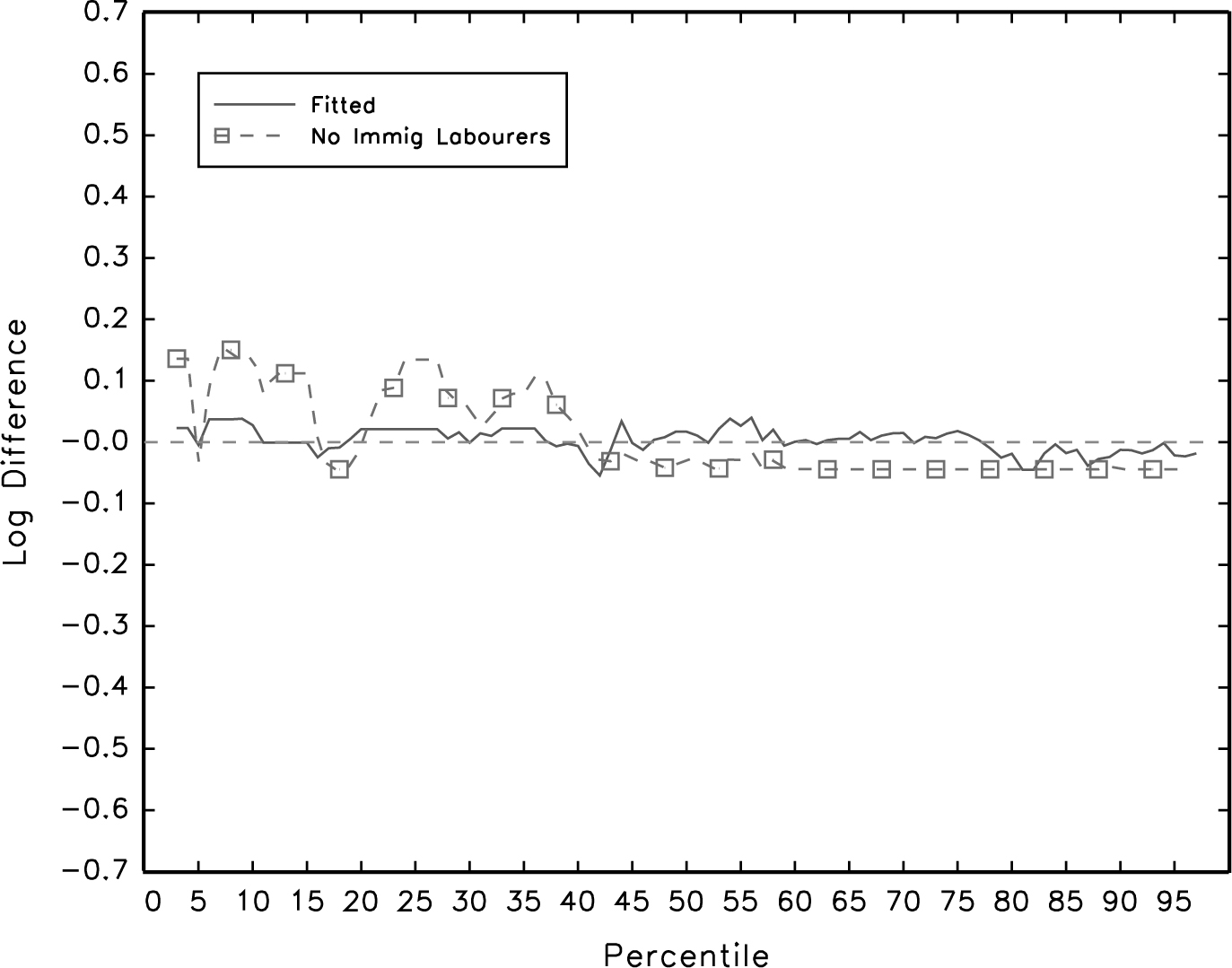
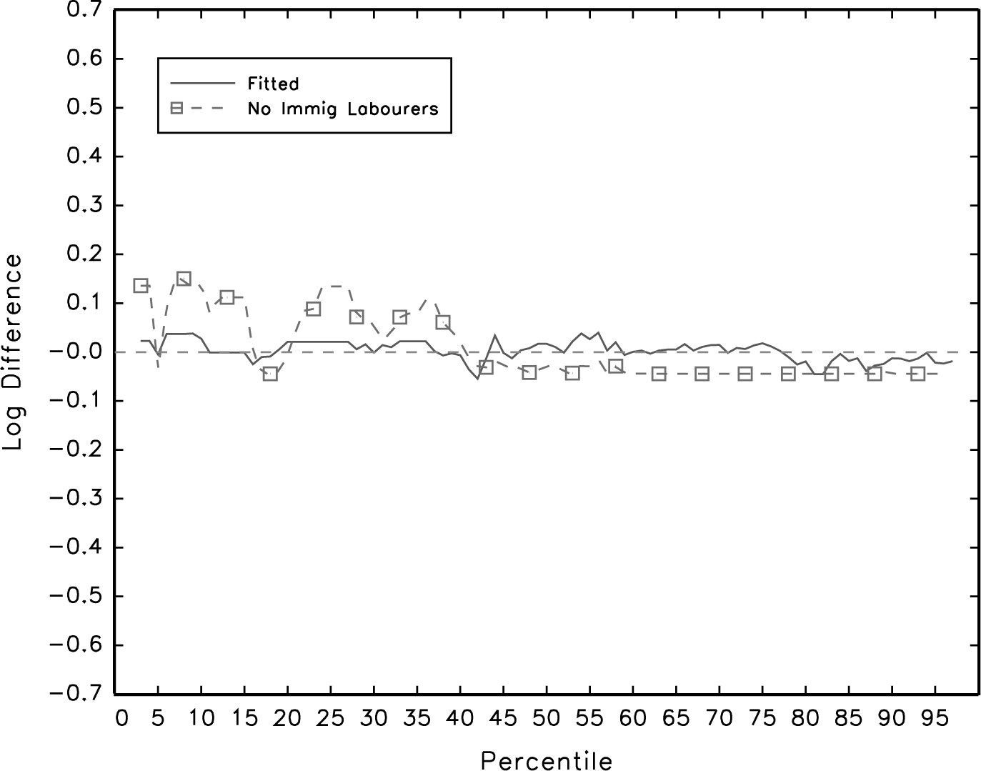
FITTED AND COUNTERFACTUAL DIFFERENCES WITH NO RECENT IMMIGRANT LABOURERS: MALE EARNINGS, 1921–1931
DIFFERENCES IN LOG PERCENTILES BETWEEN COUNTERFACTUAL AND FITTED DISTRIBUTIONS, MALE EARNINGS, 1931
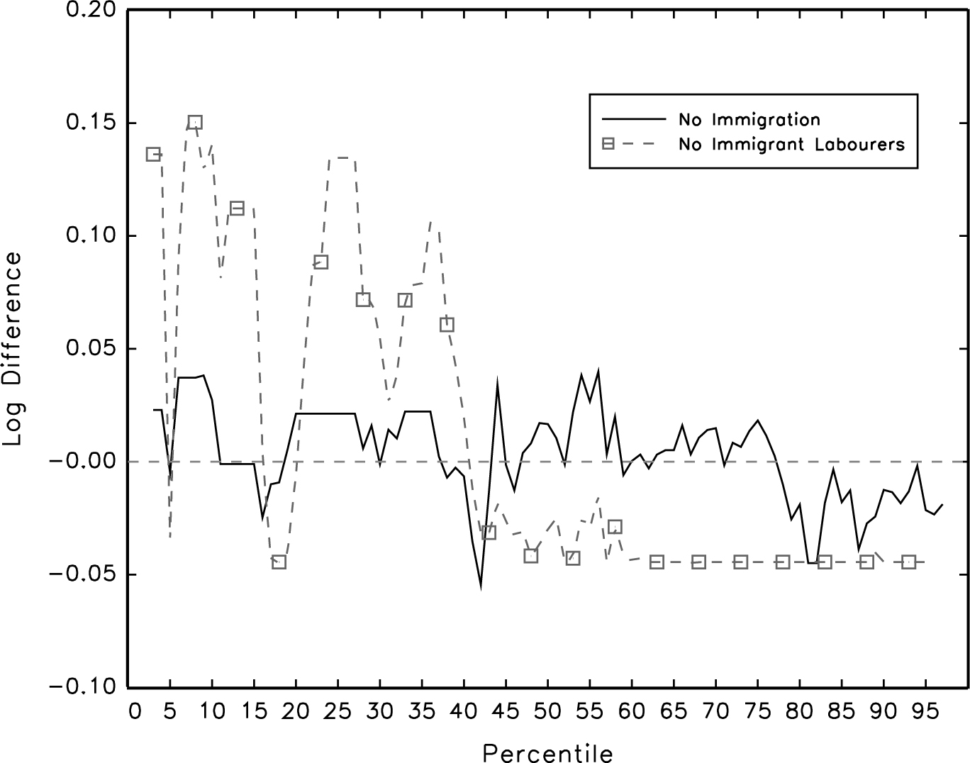
In Figure 5b, we plot differences corresponding to the counterfactual in which we eliminate only recent immigrant labourers. The implied effects of the labourers alone are substantial. Below the 40th percentile, removing the labourer inflow would have resulted in an average increase in native born real earnings of nearly 10 percentage points. Again, this can be seen clearly in the plots relative to the fitted 1931 distribution in Figure 6. There, one can also see the spillover impact of removing immigrant labourers on wages in other occupations. In particular, real earnings in occupations with above median wages would have fallen by approximately 5 percent. This highlights the arguments of OP that one needs to look beyond narrow occupation groups to measure the full impact of immigration. It also implies that the impact of low skilled immigration alone was to substantially increase inequality. The growth in the difference between the log 90th and 10th percentiles in the 1920s would have been reduced by nearly one-third if no immigrant labourers had been admitted. The growth in the 50–10 differential would have been reduced by more than 50 percent.
We can use different predicted impacts on farm labourers under various scenarios as a means of highlighting the extent of the adjustment channels to an immigrant inflow. In the Online Appendix, we present estimates of the main specification from George J. Borjas (Reference Borjas2003) in which we regress decadal changes in native born wages on the proportional increase in farm labour that is due to recent immigration.Footnote 18 This specification can be interpreted as yielding estimates of the elasticity of demand if immigrants and native born workers were perfect substitutes and each occupation represents a separate labour market. That is, the estimated effects can be seen as reflecting immigrant effects on earnings when there are no further general equilibrium effects. Using the narrow occupation groupings in order to match with our more structural estimation, the estimated coefficient on the proportion of workers who arrived in the previous decade is −0.35. If all the immigrants who arrived in the 1920s had remained in Canada and in their intended occupation, the inflow of new immigrants over the 1920s would have implied a 158 percent increase in the farm workforce and thus a 42 percent decline in worker earnings in that sector.Footnote 19 However, the actual number of farm workers in 1931 who were immigrants that had arrived in the previous decade (i.e., the number after accounting for adjustments through re-migration and occupational switching) amounted to a 39 percent increase in the farm workforce, and thus would imply a 13 percent decline in farm worker earnings in the absence of other general equilibrium effects. Finally, making use of our production function parameter estimates and the full set of immigration inflows, our first counterfactual implies that the total immigration inflow implied a 4 percent drop in farm worker earnings. The reduction from a 13 percent to a 4 percent effect represents the impact from taking account of general equilibrium adjustments in the economy.
The counterfactual with no immigration implies that immigration had only limited impacts on the location of the native born earnings distribution. This fits with findings in David H. Pope and Glenn Withers (Reference Pope, Withers, Hatton and Williamson1994) for Australia and David Greasley and Les Oxley (Reference Greasley and Oxley2004) for Australia. Alan M. Taylor and Jeffrey G. Williamson (Reference Taylor and Jeffrey G.1997) and Timothy J. Hatton and Williamson (Reference Hatton and Jeffrey G.1998) generate much larger wage impacts from immigration using Computational General Equilibrium (CGE) models with capital held fixed, but those impacts are reduced by as much as 75 percent once capital is allowed to follow labour. Green and Gordon Sparks (Reference Green and Sparks1999) find evidence of such endogenous capital inflows for Canada before WWI using a co-integration methodology. A finding of immigration having small impacts on native born wages also fits with the literature examining recent immigration (e.g., Ottaviano and Peri (Reference Ottaviano and Peri2012)). Dustmann and Preston (Reference Dustmann and Preston2011) argue that the type of method we use can understate immigration impacts because apparently skilled immigrants based on their reported education actually compete for jobs with less skilled native born workers. Because we match immigrants to the native born in terms of the occupations they actually work in and because immigrant and native born occupational distributions are very similar, this is unlikely to be a problem here. We conclude that large inflows in specific occupations can have substantial impacts on the wages in that occupation and in closely substitutable occupations but those impacts can be mitigated by positive spill-over effects due to the arrival of a wider set of immigrants. In our case, the effects of those other immigrants implies near zero net effects of immigration even in low skilled occupations.
CONCLUSION
Using newly available micro Census data, we have shown that the Canadian earnings structure underwent a substantial increase in inequality between 1911 and 1941, with most of the increase occurring between 1921 and 1931. Given that the immigrant inflow in the 1920s was particularly low skilled, it seems plausible that there was a connection between immigration and the increase in inequality in that decade. Our conclusion, however, is that immigration played a minor role as a driver of the changes in the earnings structure. We show that this happened largely because of adjustments made by immigrants themselves. In the 1910s, when there was little policy control over immigration, the people who chose to immigrate to Canada were those with skills that matched the occupational demand in the economy. This is evident in the fact that their occupational distribution was similar to the native born at the time they entered Canada. In contrast, in the 1920s, the government actively shaped immigration, with the result that the inflow was dominated by farmers and farm labourers. But by the end of that decade, recent immigrants had shifted occupations such that their occupational distribution looked similar to that of the native born. In both decades, with the immigrant occupational distribution being similar to that of the native born, we would expect the immigrant inflow to affect the level of the earnings distribution much more than its shape. In addition to these adjustments, there were general equilibrium effects of immigration on wages that also served to spread out the effects of the mass immigration. Our estimates imply that without any adjustment, immigration would have reduced the wage for farm labour by 42 percent in the 1920s but with all the adjustment channels, the ultimate impact was a reduction of only 4 percent. Of this 38 percent reduction in the wage effect, three-quarters was due to geographic and occupational adjustments made by the immigrants themselves and one quarter was because of general equilibrium price adjustments. Thus, the driving force for the substantial increase in inequality in Canada in this era must have been something other than immigration.
 , where Δln(wNjkt
) is the change in native born log earnings in occupation j and age group k, ΔLIjkt
corresponds to the number of recent immigrants who were in that occupation and age category in the time t (e.g., 1931) Census, and LNjkt–
1 + LIjkt–
1 is the total number of workers (native born and immigrant) who were working in that occupation by age cell in the t − 1 Census (1921 in this example). Note that the regression is based on Census data and thus the immigrant employment numbers are after immigrant adjustments.