1. Introduction
Flows characterised by strong stable density stratification are encountered in many geophysical applications. In the atmosphere, boundary layers with strong static stability are observed in polar regions or during clear nights as a result of strong cooling at the ground (Nieuwstadt Reference Nieuwstadt1984; van de Wiel et al. Reference van de Wiel, Ronda, Moene, Bruin and Holtslag2002; Grachev et al. Reference Grachev, Fairall, Persson, Andreas and Guest2005). In the oceans, pycnoclines are similarly characterised by large density gradients due to variations in the temperature and salinity profiles (Taylor & Sarkar Reference Taylor and Sarkar2007). Under such strongly stratified conditions, turbulence can be virtually absent for a long period of time and then occur intermittently at other times in strong bursts (Kondo, Kanechika & Yasuda Reference Kondo, Kanechika and Yasuda1978).
In order to classify observations of the stable atmospheric boundary layer, Mahrt et al. (Reference Mahrt, Sun, Blumen, Delany and Oncley1998) proposed two dynamical regimes which he referred to as the ‘weakly stable’ regime and the ‘very stable’ regime. In the weakly stable regime, the stabilising effect of stratification is not strong enough to suppress turbulence and continuously turbulent states are typically observed. The resulting regime is relatively well understood, and theoretical approaches, such as the self-similarity theory of Monin–Obhukov (Monin & Obukhov Reference Monin and Obukhov1954; Obukhov Reference Obukhov1971), provide a satisfactory agreement with observations. On the other hand, the strongly stable regime is less well understood and more challenging to model.
Perhaps one of the most important and poorly understood issues is the characterisation of mixing processes. Although many models assume a fixed ratio between buoyancy flux and kinetic energy dissipation of approximately 0.2 (Osborn Reference Osborn1980; Wunsch & Ferrari Reference Wunsch and Ferrari2004), there is very large uncertainty as to what the mixing efficiency is and, indeed, whether it is constant (e.g. Smyth, Moum & Caldwell Reference Smyth, Moum and Caldwell2001). Linden (Reference Linden1979) reported experimental observations of the mixing efficiency quantified by the flux Richardson number
 $\mathit{Ri}_{f}$
, defined as the ratio of the conversion rate from kinetic to potential energy to the turbulent kinetic energy injection rate due to shear. Although a rather large spread of data was observed,
 $\mathit{Ri}_{f}$
was found to increase with the bulk Richardson number,
 $\mathit{Ri}$
, up to a maximum of
 $\mathit{Ri}_{f}\approx 0.2$
for
 $\mathit{Ri}\lesssim 0.1{-}0.15$
and decrease for larger values of
 $\mathit{Ri}$
. As originally argued by Phillips (Reference Phillips1972), if the buoyancy flux decreases with stratification at relatively large static stability, there is an effectively negative eddy diffusivity. As a result, small perturbations in the density profile are unstable and lead to the creation of sharp interfaces between relatively well-mixed layers, a rather striking feature observed in a number of experiments of stably stratified flows (Ruddick, McDougall & Turner Reference Ruddick, McDougall and Turner1989; Park, Whitehead & Gnanadeskian Reference Park, Whitehead and Gnanadeskian1994; Holford & Linden Reference Holford and Linden1999). Recent experiments by Oglethorpe, Caulfield & Woods (Reference Oglethorpe, Caulfield and Woods2013) have also suggested the presence of a plateau in the mixing efficiency for large stratifications, possibly connected to self-similar regimes of strongly stratified turbulence (Billant & Chomaz Reference Billant and Chomaz2001).
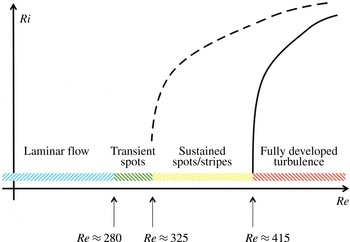
Sketch of the intermittency boundary (solid line) and the relaminarisation boundary (dashed line) in the
 $\mathit{Re}{-}\mathit{Ri}$
plane of Couette flows.

More importantly, it is unclear how the mixing efficiency is influenced by the appearance of global intermittency characterising strongly stratified regimes (van de Wiel et al.
Reference van de Wiel, Ronda, Moene, Bruin and Holtslag2002; van de Wiel, Moene & Jonker Reference van de Wiel, Moene and Jonker2012) where laminar and turbulent regions coexist and mutually interact. Although strongly stratified flows are known to be highly intermittent (Rorai, Mininni & Pouquet Reference Rorai, Mininni and Pouquet2014), large-scale intermittency and coexistence of laminar and turbulent dynamics may also arise in unstratified conditions at low Reynolds number,
 $\mathit{Re}$
, due to viscous effects ‘quenching’ the turbulence. Coles (Reference Coles1965) conducted a number of Taylor–Couette flow (TCF) experiments investigating the transition from laminar finite-amplitude instabilities to turbulence. Intermittent states were observed, characterised by spiral bands of turbulence alternating with laminar regions. More recently, Prigent et al. (Reference Prigent, Grégoire, Chaté, Dauchot and van Saarloos2002) also performed experiments on more extended domains, showing the existence of similar large-scale modulations in both plane Couette flow (PCF) and TCF for
 $340<\mathit{Re}<415$
, where
 $\mathit{Re}=U\,h/{\it\nu}$
is here defined using half the velocity difference
 $U$
, the half channel gap
 $h$
and the kinematic viscosity of the fluid
 ${\it\nu}$
. The appearance of inclined bands of laminar/turbulent regions has recently been studied numerically, both in small aspect-ratio domains perpendicular to the bands (Barkley & Tuckerman Reference Barkley and Tuckerman2005, Reference Barkley and Tuckerman2007) and in extended domains (Duguet, Schlatter & Henningson Reference Duguet, Schlatter and Henningson2010).
Similar structures have also been found at higher
 $\mathit{Re}$
when a stabilising force other than viscosity suppresses turbulent motions. García-Villalba & del Álamo (Reference García-Villalba and del Álamo2011) reported intermittent dynamics in stratified channel flows in the form of laminar spots surrounded by turbulent dynamics. Brethouwer, Duguet & Schlatter (Reference Brethouwer, Duguet and Schlatter2012) showed coexistence of laminar/turbulent inclined bands in spanwise rotating Couette flow and in channel flows subjected to buoyancy or magnetic forces. Ansorge & Mellado (Reference Ansorge and Mellado2014) and Deusebio et al. (Reference Deusebio, Brethouwer, Schlatter and Lindborg2014) found inclined turbulent/laminar stripes in stratified Ekman layers, i.e. boundary layers developing under the effect of wall-normal rotation, which indicates that turbulent patterns might be more general and not limited to TCF and PCF dynamics only.
The introduction of a stabilising force into the system, such as stratification, allows us to have an additional control parameter to study the complexity arising from the temporal and spatial intermittency of the flow. Figure 1 shows a cartoon of the phase space of stably stratified PCF where two dimensionless parameters control the dynamics, the bulk Reynolds number
 $\mathit{Re}$
and the bulk Richardson number
 $\mathit{Ri}$
. The two lines show the intermittency boundary (solid line) between fully developed turbulence and intermittent regimes, which crosses the zero-stratification axis at approximately
 $\mathit{Re}=415$
(Prigent et al.
Reference Prigent, Grégoire, Chaté, Dauchot and van Saarloos2002; Duguet et al.
Reference Duguet, Schlatter and Henningson2010), and the relaminarisation boundary (dashed line) to the left of which no chaotic attractor exists, crossing the zero-stratification axis at approximately
 $\mathit{Re}=324$
(Duguet et al.
Reference Duguet, Schlatter and Henningson2010). At the present stage it is not known where the regime boundaries lie in the
 $\mathit{Re}{-}\mathit{Ri}$
plane, and the main aim of the current investigation is to be able to identify the intermittency boundary. On the other hand, tracing the relaminarisation boundary is beyond the scope of the present study, although there have been some recent investigations of this issue focusing on the identification of minimal seeds (Eaves & Caulfield Reference Eaves and Caulfield2015) and edge states (Olvera & Kerswell Reference Olvera and Kerswell2014) in stably stratified PCF. The two boundaries are distinct and well separated at low
 $\mathit{Re}$
. Nevertheless, it is unclear whether they would approach each other and possibly coalesce at higher
 $\mathit{Re}$
.
The quest to trace out these boundaries is connected with the development of an understanding of the relaminarisation process and the maintenance of wall-bounded turbulence. Early approaches, such as the Miles–Howard criterion (Howard Reference Howard1961; Miles Reference Miles1961), related relaminarisation to either linear stability analysis of shear flows or to the balance between turbulent kinetic energy production by shear and conversion to potential energy (e.g. Armenio & Sarkar Reference Armenio and Sarkar2002). Nieuwstadt (Reference Nieuwstadt2005) presented evidence that the relaminarisation of open-channel flows subject to strong cooling at the lower wall occurs when
 $h/L\approx 0.5$
, where
 $h$
is the half channel gap and
 $$\begin{eqnarray}L=u_{{\it\tau}}^{3}/C_{{\it\kappa}}q_{w}\end{eqnarray}$$
is the Obukhov length scale (Monin & Obukhov Reference Monin and Obukhov1954), with
 $u_{{\it\tau}}^{2}={\it\rho}_{0}{\it\tau}_{w}$
being the friction velocity,
 $C_{{\it\kappa}}\approx 0.4$
the von Kármán constant,
 $q_{w}$
the wall heat flux and
 ${\it\tau}_{w}$
the shear stress at the wall. Flores & Riley (Reference Flores and Riley2010) suggested, however, that the critical value of
 $h/L$
may be
 $\mathit{Re}$
-dependent and proposed that a criterion based on
 $L^{+}$
should instead be used, where
 $L^{+}=Lu_{{\it\tau}}/{\it\nu}$
is the Monin–Obukhov length scale normalised in wall units.
From a physical point of view, the
 $L^{+}$
criterion suggests that relaminarisation is inherently a near-wall process for wall-bounded flows. The importance of near-wall dynamics to sustain wall-bounded turbulence in unstratified flows has been recognised for a long time. The region close to the wall is the place where most of the turbulent kinetic energy is generated (near
 $y=15{\it\nu}/u_{{\it\tau}}$
) and fluctuations are the largest (see, for instance, Kim, Moin & Moser Reference Kim, Moin and Moser1987). Hamilton, Kim & Waleffe (Reference Hamilton, Kim and Waleffe1995) identified a self-sustained near-wall process in which counter-rotating streamwise vortices produce high- and low-velocity streaks by advecting the mean flow. These streaks are unstable in the inviscid limit and their secondary instability leads to the formation of new streamwise vortices, hence the cycle. The importance of the so-called near-wall cycle in wall-bounded turbulent dynamics has also been emphasised by synthetic simulations in which horizontally periodic boxes were reduced until turbulence could no longer be sustained (Jiménez & Moin Reference Jiménez and Moin1991). The spanwise extent of the minimal flow unit, i.e. the smallest box size able to allow the development of turbulent flows, was found to be of the order of the near-wall streak spacing. Jiménez & Pinelli (Reference Jiménez and Pinelli1999) extended this to the vertical direction by damping out turbulent fluctuations above a certain height
 ${\it\delta}$
and showed that turbulence can only be sustained if
 ${\it\delta}>60{\it\nu}/u_{{\it\tau}}$
.
Here, we will provide evidence that suggests that the onset of intermittency in strongly stratified PCF is indeed connected with the suppression of the near-wall cycle and that the criterion proposed by Flores & Riley (Reference Flores and Riley2010) based on
 $L^{+}$
can capture the onset of intermittent dynamics in the asymptotic regime of high-
 $\mathit{Re}$
stably stratified PCF. When the flow is indeed turbulent, we also investigate the efficiency of mixing using several definitions of the flux Richardson number
 $\mathit{Ri}_{f}$
. When
 $\mathit{Ri}_{f}$
is defined in terms of global quantities describing the energy input by the wall forcing and the buoyancy flux through the boundaries, we find that
 $\mathit{Ri}_{f}$
increases linearly with
 $\mathit{Ri}$
, due to the fact that the mean velocity and density profiles are related by
 $q_{w}/T\approx {\it\tau}_{w}/U$
in the canonical geometry of PCF. We have also found that appropriate measures of
 $\mathit{Ri}_{f}$
take close to the same values in both laminar and turbulent regions of the flow when it is spatially intermittent. Although there has been recent interesting work considering in detail the most appropriate measure of mixing efficiency (see, for example, Karimpour & Venayagamoorthy Reference Karimpour and Venayagamoorthy2015; Salehipour & Peltier Reference Salehipour and Peltier2015), since we are focused on intermittency, we believe that slight modifications of the classical definition of the flux Richardson number adequately capture the (interestingly weak) effect of intermittency on the ‘efficiency’ of mixing.
Consistent with this observation, we confirm that Monin–Obukhov theory is able to provide a reasonable description of the velocity and temperature mean profiles, comparable to more sophisticated models such as the explicit algebraic model (EAM) developed by Lazeroms et al. (Reference Lazeroms, Brethouwer, Wallin and Johansson2013). We then use these models to predict the intermittency boundary in the
 $\mathit{Re}{-}\mathit{Ri}$
phase space separating the intermittent and fully developed turbulent regimes, and demonstrate good agreement between these predictions and the results of our numerical simulations.
The paper is organised as follows: § 2 gives a summary of the numerical code and an overview of the simulations; § 3 presents mean global quantities and turbulent fluctuations; § 4 describes phenomenologically the intermittent regimes of PCF; § 5 investigates the efficiency of mixing considering different definitions of
 $\mathit{Ri}_{f}$
; in § 6 we develop an analytical model based on Monin–Obukhov self-similarity theory and an EAM to predict the boundary between fully turbulent and intermittent dynamics and we compare this prediction with our simulations; finally, § 7 provides conclusions and final remarks.
2. Numerical set-up
We consider a temperature-stratified system described by the Navier–Stokes equations under the Boussinesq approximation where density variations are related to temperature variations via a linear equation of state, i.e.
 $$\begin{eqnarray}\displaystyle & \displaystyle \frac{\partial \boldsymbol{u}}{\partial t}+\boldsymbol{u}\boldsymbol{\cdot }\boldsymbol{{\rm\nabla}}\boldsymbol{u}=-\frac{\boldsymbol{{\rm\nabla}}p}{{\it\rho}_{0}}+{\it\nu}{\rm\nabla}^{2}\boldsymbol{u}-g{\it\alpha}_{V}T\boldsymbol{e}_{y}, & \displaystyle\end{eqnarray}$$
 $$\begin{eqnarray}\displaystyle & \displaystyle \frac{\partial T}{\partial t}+\boldsymbol{u}\boldsymbol{\cdot }\boldsymbol{{\rm\nabla}}T={\it\kappa}{\rm\nabla}^{2}T, & \displaystyle\end{eqnarray}$$
 $$\begin{eqnarray}\displaystyle & \boldsymbol{{\rm\nabla}}\boldsymbol{\cdot }\boldsymbol{u}=0. & \displaystyle\end{eqnarray}$$
 $\boldsymbol{u}=(u,v,w)$
is the velocity vector in the reference system
 $(x,y,z)$
with
 $x$
and
 $z$
being the horizontal coordinates and
 $y$
the vertical coordinate,
 $p$
is the pressure,
 ${\it\rho}_{0}$
is the background reference density,
 $T$
is the temperature and
 $g\,{\it\alpha}_{V}$
is the ‘buoyancy parameter’, with
 ${\it\alpha}_{V}$
being the thermal expansion coefficient and
 $g$
the gravity. The molecular kinematic viscosity
 ${\it\nu}$
and thermal diffusivity
 ${\it\kappa}$
are assumed to be constant.
Periodic boundary conditions are imposed in the
 $x$
and
 $z$
directions. In the vertical direction, the velocity and the temperature satisfy Dirichlet boundary conditions at the two counter-moving walls, i.e.
 $$\begin{eqnarray}u=-U,\quad v=0,\quad w=0,\quad T=-T_{r}\end{eqnarray}$$
at
 $y=-h$
and
 $$\begin{eqnarray}u=U,\quad v=0,\quad w=0,\quad T=T_{r}\end{eqnarray}$$
at
 $y=h$
. When not otherwise stated, in the following we will always refer to the dimensionless counterparts of the quantities which have been normalised using
 $U$
as a reference velocity,
 $T_{r}$
as a reference temperature and
 $h$
as a reference length. The dynamics can be described in terms of three dimensionless parameters: the bulk Reynolds number
 $\mathit{Re}$
,
 $$\begin{eqnarray}\mathit{Re}=\frac{Uh}{{\it\nu}},\end{eqnarray}$$
the bulk Richardson number,
 $$\begin{eqnarray}\mathit{Ri}=\frac{g{\it\alpha}_{V}T_{r}h}{U^{2}},\end{eqnarray}$$
and the Prandtl number,
 $$\begin{eqnarray}\mathit{Pr}=\frac{{\it\nu}}{{\it\kappa}}.\end{eqnarray}$$
Here, we consider
 $\mathit{Pr}=0.7$
as a model of temperature stratification in air. It is important to note that the wall shear stress
 $$\begin{eqnarray}{\it\tau}_{w}={\it\nu}\left.\frac{\partial u}{\partial y}\right|_{y=\pm 1}\end{eqnarray}$$
and heat flux
 $$\begin{eqnarray}q_{w}={\it\kappa}\left.\frac{\partial T}{\partial y}\right|_{y=\pm 1}\end{eqnarray}$$
are not prescribed but naturally arise from the dynamics. As a consequence, the friction Reynolds number, defined using the friction velocity
 $u_{{\it\tau}}=\sqrt{{\it\tau}_{w}/{\it\rho}_{0}}$
,
 $$\begin{eqnarray}\mathit{Re}_{{\it\tau}}=\frac{u_{{\it\tau}}h}{{\it\nu}}\quad \text{with }{\it\rho}_{0}u_{{\it\tau}}^{2}={\it\tau}_{w},\end{eqnarray}$$
which quantifies the ratio between the largest scales
 ${\sim}h$
and the smallest scales
 ${\sim}{\it\nu}/u_{{\it\tau}}$
, and the Nusselt number,
 $$\begin{eqnarray}\mathit{Nu}=\frac{q_{w}h}{{\it\kappa}T_{r}},\end{eqnarray}$$
used to estimate the heat transfer are unknown a priori and are to be considered as output parameters.
Equations (2.1) together with the boundary conditions (2.2)–(2.3) have been discretised using Fourier modes in the two horizontal directions and second-order finite differences in the vertical direction. Time stepping was achieved by means of a low-storage third-order Runge–Kutta method for the nonlinear terms and a semi-implicit Crank–Nicolson method for updating viscous and diffusive terms. Nonlinear terms were evaluated in physical space and a 2∕3 dealiasing rule was applied when transforming back to Fourier space. Variable time steps based on a Courant–Friedrichs–Lewy (CFL) number equal to 0.5 were employed. For further details on the numerical scheme we refer the interested reader to Taylor (Reference Taylor2008) and Bewley (Reference Bewley2010). In order to carry out high-resolution numerical simulations, the code was parallelised by using a 2D domain decomposition and parallel transpose operations. Good scalability was observed up to a few thousand processors.
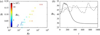
Figure 2 shows a summary in the
 $\mathit{Re}{-}\mathit{Ri}$
plane of the simulations which did not relaminarise within the used time window (in all the cases larger than 1000
 $h/U$
, corresponding to 10–
 $20h/u_{{\it\tau}}$
). The simulations span more than two orders of magnitude in
 $\mathit{Re}$
and values of
 $\mathit{Ri}$
that range between 0 and 0.175. Similarly to the simulations of García-Villalba, Azagra & Uhlmann (Reference García-Villalba, Azagra and Uhlmann2011), in runs 1 to 16 in table 1 we consider sets of
 $\mathit{Re}{-}\mathit{Ri}$
values that keep
 $\mathit{Re}_{{\it\tau}}$
approximately constant. Simulations were initialised by fixing
 $\mathit{Ri}$
and adjusting
 $\mathit{Re}$
every 100 time steps such that the target value of
 $\mathit{Re}_{{\it\tau}}$
was achieved. This allowed us to find an estimate of
 $\mathit{Re}$
which was then held fixed. The reason for fixing
 $\mathit{Re}_{{\it\tau}}$
rather than
 $\mathit{Re}$
is twofold: first, it is
 $\mathit{Re}_{{\it\tau}}$
that imposes the requirements for a fully resolved simulation; second, it is
 $\mathit{Re}_{{\it\tau}}$
that defines the ratio between largest and smallest scales.
(a) Summary of the simulations (listed in table 1), in the
 $\mathit{Re}{-}\mathit{Ri}$
plane. Colours represent the magnitude of the
 $\mathit{Re}_{{\it\tau}}$
, ranging from 40 (blue) to 1500 (red); (b)
 $\mathit{Re}_{{\it\tau}}$
for the same set of parameters of simulation 2 for different box sizes: ——,
 $(L_{x},L_{z})=(8{\rm\pi},4{\rm\pi})$
; - - - -,
 $(L_{x},L_{z})=(16{\rm\pi},8{\rm\pi})$
;
 $\cdots \cdots$
,
 $(L_{x},L_{z})=(32{\rm\pi},16{\rm\pi})$
.

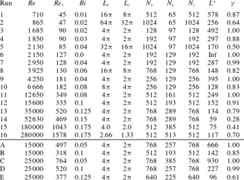
Summary of the characteristics of the simulations.

Eight values of
 $\mathit{Re}_{{\it\tau}}$
were chosen, ranging from 45 (close to the value of unstratified relaminarisation) up to 1500. Two sets of simulations at constant
 $\mathit{Re}=1.5\times 10^{4}$
and
 $\mathit{Re}=2.5\times 10^{4}$
were also run (runs from A to E in table 1). Figure 2(a) shows
 $\mathit{Re}_{{\it\tau}}$
by the colour of the open circles marking the
 $\mathit{Re}{-}\mathit{Ri}$
plane. As is evident, constant-
 $\mathit{Re}_{{\it\tau}}$
contours are sloped lines at increasing
 $\mathit{Re}$
and increasing
 $\mathit{Ri}$
. We increase
 $\mathit{Ri}$
until (partially) turbulent states cannot be sustained and full relaminarisation is achieved. As shown in figure 2(a), relaminarisation occurs at larger
 $\mathit{Ri}$
as
 $\mathit{Re}_{{\it\tau}}$
(and
 $\mathit{Re}$
) increases.
Table 1 lists the numerical parameters of the simulations. Here,
 $N_{x}$
,
 $N_{y}$
and
 $N_{z}$
represent the number of points in physical space along the streamwise, wall-normal and spanwise directions respectively;
 ${\it\gamma}$
represents the fraction of the flow considered to be turbulent, and its actual definition will be further discussed in § 4.2;
 $L^{+}$
represents the ratio between the Monin–Obukhov length scale (Obukhov Reference Obukhov1971; Monin & Obukhov Reference Monin and Obukhov1954),
 $$\begin{eqnarray}L=\frac{u_{{\it\tau}}^{3}}{C_{{\it\kappa}}q_{w}},\end{eqnarray}$$
and the wall viscous length scale,
 $l={\it\nu}/u_{{\it\tau}}$
, i.e.
 $$\begin{eqnarray}L^{+}=\frac{L}{l}=\frac{u_{{\it\tau}}L}{{\it\nu}},\end{eqnarray}$$
where
 $C_{{\it\kappa}}$
in (2.11) is the von Kármán coefficient, i.e.
 $C_{{\it\kappa}}\approx 0.4$
. From a physical point of view, the Monin–Obukhov length scale
 $L$
is a measure of the distance from the wall at which buoyancy forces affect the dynamics, where injection of turbulent kinetic energy and conversion to potential energy are of similar magnitude, whereas
 $l$
is the relevant length scale for near-wall dynamics. The results at
 $\mathit{Re}_{{\it\tau}}=130$
and
 $\mathit{Re}_{{\it\tau}}\approx 540$
were found to be in agreement with the simulations of García-Villalba et al. (Reference García-Villalba, Azagra and Uhlmann2011), thus providing a validation of the numerical tool used in the present investigation. When feasible, several box sizes were considered in order to check the convergence as well as the sensitivity of our results with respect to the box dimensions. Table 1 only summarises the simulations with the largest horizontal extents. For the lowest friction Reynolds numbers, we consider computational domains as large as
 $L_{x}=200h$
and
 $L_{z}=100h$
, producing sustained inclined striped patterns similar to those observed by Barkley & Tuckerman (Reference Barkley and Tuckerman2005), Brethouwer et al. (Reference Brethouwer, Duguet and Schlatter2012) and Duguet & Schlatter (Reference Duguet and Schlatter2013).
Following general guidelines for direct numerical simulations of wall-bounded turbulence (Moin & Mahesh Reference Moin and Mahesh1998), we adjust the grid spacing such that
 ${\rm\Delta}x^{+}\approx 8$
,
 ${\rm\Delta}z^{+}\approx 4$
and
 $y_{10}^{+}<10$
, where
 $y_{10}$
is the tenth point from the wall and the
 $+$
superscript represents quantities normalised using viscous scaling, i.e. using
 $l$
for length scales and
 $u_{{\it\tau}}$
for velocities. As
 $\mathit{Re}_{{\it\tau}}$
increases, the grid spacing required to resolve the smallest turbulent length scales decreases, making it necessary to reduce the size of the computational domain in order to reduce the computational cost. It is important to appreciate that our results may be dependent on the size of the computational domain and that the dimensions considered in some simulations (e.g. 15 and 16 in table 1) may well be close to marginal, according to the guidelines provided by Flores & Jiménez (Reference Flores and Jiménez2010). However, as we will discuss below, these simulations allow us to gain some insight into the intermittent dynamics and an estimate of the intermittency at high
 $\mathit{Re}$
despite the reduced dimensions. The smallest computational domain considered (at
 $\mathit{Re}_{{\it\tau}}=1500$
) has
 $L_{x}=2.67h$
and
 $L_{z}=1.33h$
, corresponding in viscous units to
 $L_{x}^{+}\approx 4000$
and
 $L_{z}^{+}\approx 2000$
.
The size of the computational domain affects the results significantly only when coexistence between laminar and turbulent patches arises. Figure 2(b) shows the time evolution of
 $\mathit{Re}_{{\it\tau}}$
for a simulation at
 $\mathit{Re}=865$
and
 $\mathit{Ri}=0.02$
. For a small computational domain size, turbulence cannot be sustained and full relaminarisation is observed. When the computational domain is marginal, the flow stays turbulent, but it exhibits temporal intermittency with large fluctuations (approximately 5–10 %) of
 $\mathit{Re}_{{\it\tau}}$
. As the size of the computational domain increases, temporal intermittency is suppressed and replaced by spatial intermittency. Interestingly, we find that time averages of global quantities (such as
 $\mathit{Re}_{{\it\tau}}$
,
 $\mathit{Nu}$
and the turbulent fraction
 ${\it\gamma}$
) vary only by a few per cent with the size of the computational domain as long as the flow stays at least partially turbulent. In particular, we find that for the case in figure 2(b) (simulation 2) the time-averaged turbulent fraction
 ${\it\gamma}$
in various domains varies between 60 % and 65 %. However, we find that the size of the computational domain significantly affects the qualitative patterns of the laminar/turbulent patches in the intermittent regime. Turbulent and laminar patches tend to be aligned in the streamwise direction in small computational domains, whereas as the domain size increases, inclined laminar/turbulent bands similar to the findings of Duguet et al. (Reference Duguet, Schlatter and Henningson2010) are found.
3. One-point statistics
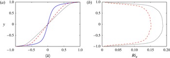
Figure 3(a) shows the mean streamwise velocity profiles
 $\langle \overline{u}\rangle$
for three different simulations at increasing
 $\mathit{Re}$
and
 $\mathit{Ri}$
. In the following, we will use the overbar
 $\overline{\cdot }$
to denote a horizontal average and the brackets
 $\langle \cdot \rangle$
to denote the time average extending over the entire simulation. As
 $\mathit{Ri}$
increases, a constant-shear region appears in the core of the flow. It is worth noting that this region is still turbulent and the observed linear profile results from stratified turbulent dynamics rather than from a purely laminar flow. The development of a constant-shear region can be explained by a suppression of the local turbulent length scale by stratification. If the interior flow is independent of the distance from the walls, the turbulence, and hence the shear, is only determined by local properties (momentum and buoyancy fluxes) which are constant along
 $y$
. It should be noted, however, that since the wall stress provides the driving force for turbulence in PCF, the turbulence remains dependent on the wall stress. As
 $\mathit{Re}$
increases, the constant-shear region extends closer to the wall. Gradients at the wall do not steepen extensively because of the balancing effect of stratification which causes
 $\mathit{Re}_{{\it\tau}}$
to increase from 130 to 520 in spite of the much larger change in
 $\mathit{Re}$
, from 2150 to 35 000.
Vertical profiles of (a)
 $\langle \overline{u}\rangle$
and (b)
 $\mathit{Ri}_{g}$
: simulation 6 (——), simulation 11 (- - - -) and simulation 13 (
 $\cdots \cdots$
).

The density profiles show very similar behaviour to the velocity, which is expected due to the fact that the
 $\mathit{Pr}$
is close to unity,
 $\mathit{Pr}=0.7$
. Figure 3(b) shows the time-averaged gradient Richardson number,
 $$\begin{eqnarray}\mathit{Ri}_{g}(y)=\mathit{Ri}\frac{\displaystyle \left\langle \frac{\partial \overline{T}}{\partial y}\right\rangle }{\displaystyle \left\langle \left(\frac{\partial \overline{u}}{\partial y}\right)^{2}\right\rangle }.\end{eqnarray}$$
The gradient Richardson number, as defined in (3.1), is minimum at the wall and increases towards the centre of the channel. Using the background method (Doering & Constantin Reference Doering and Constantin1992), Tang, Caulfield & Kerswell (Reference Tang, Caulfield and Kerswell2009) identified optimal profiles that maximise buoyancy flux in stratified PCF subject only to global energetic balances and a constraint on the horizontal momentum, and found non-monotonic profiles of
 $\mathit{Ri}_{g}$
exhibiting a local maximum close to the walls. The
 $\mathit{Ri}_{g}$
profiles in figure 3(b) are not in agreement with such a prediction, suggesting that the constraints imposed by Tang et al. (Reference Tang, Caulfield and Kerswell2009) are far too weak and neglect the importance of (weakly stratified) near-wall dynamics crucial to sustain turbulence in PCF.
We find that the broad plateau developing in the core of the channel increases with
 $\mathit{Ri}$
(figure 3
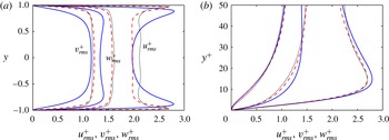
b) and saturates in amplitude for large values smaller than 0.25, i.e. the limiting threshold for linear normal-mode stability of inviscid stably stratified shear flows. Figure 4 shows the different components of the turbulent velocity fluctuations. As shown in panel (b), the dynamics close to the wall generally retains viscous scalings: the location of the near-wall peak of
 $u_{rms}$
in wall units is not significantly affected by changes in
 $\mathit{Re}$
and
 $\mathit{Ri}$
, although its intensity slightly decreases as
 $\mathit{Re}$
and
 $\mathit{Ri}$
increase. The intensity of streamwise fluctuations in the centre of the channel increases as the stratification (and the shear) in the core region increases.
Velocity fluctuations: (a) across the channel and (b) blow-up near to the wall. The line types are as in figure 3.

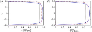
Figure 5 shows the turbulent shear stress scaled by
 $u_{{\it\tau}}^{2}$
. The decrease of the magnitude of the plateau with increasing stratification indicates that a non-negligible part of the momentum (up to 10 % for the highest
 $\mathit{Ri}$
) is transferred by molecular diffusion. Since – as we will argue below – the slopes of the mean velocity and temperature profiles are set by the stratification, at fixed
 $\mathit{Ri}$
we would expect that
 $\langle \overline{u^{\prime }v^{\prime }}\rangle /u_{{\it\tau}}^{2}$
approaches unity as
 $\mathit{Re}\rightarrow \infty$
. The turbulent heat flux (not shown) also displays very similar behaviour to the turbulent momentum flux, i.e. a constant plateau in the central region with values that asymptotically approach
 $q_{w}$
, as defined in (2.8), as the Péclet number
 $Pe=\mathit{Re}\,\mathit{Pr}\rightarrow \infty$
.
(a) Turbulent shear stress
 $-\langle \overline{u^{\prime }v^{\prime }}\rangle$
, normalised by the friction velocity,
 $u_{{\it\tau}}^{2}$
. (b) Turbulent heat flux
 $-\langle \overline{v^{\prime }T^{\prime }}\rangle$
, normalised by the wall heat flux,
 $q_{w}$
. The lines are as in figure 3.

4. Intermittent dynamics
4.1. Phenomenology of intermittency at large and low
 $\mathit{Re}$

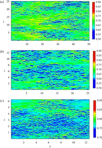
In figure 6, the streamwise velocity in a horizontal plane close to the upper wall,
 $y=0.95$
, is shown for three weakly intermittent simulations. The value of
 $\mathit{Re}_{{\it\tau}}$
increases from (a) to (c), corresponding to
 $\mathit{Re}_{{\it\tau}}=130,180$
and 520, simulations 8, 10 and 13 respectively. In all three cases, laminar patches appear in the flow, similar to those observed by García-Villalba et al. (Reference García-Villalba, Azagra and Uhlmann2011) in stratified channel flows. It should be noted that in the three cases the dimension of the box varies considerably and the laminar patches at low
 $\mathit{Re}_{{\it\tau}}$
are significantly larger. Nevertheless, the three flows exhibit similar dynamics with laminar patches cyclically appearing and disappearing in the flow with time scales of the order of hundreds of convective time units. For these simulations, spatially averaged quantities show small fluctuations in time, suggesting that the chosen box sizes are suitable to study the intermittent dynamics. The degree of stratification in these cases is not strong enough to lead to the generation of sustained and steady inclined laminar/turbulent bands as observed by Brethouwer et al. (Reference Brethouwer, Duguet and Schlatter2012) and Deusebio et al. (Reference Deusebio, Brethouwer, Schlatter and Lindborg2014). As
 $\mathit{Ri}$
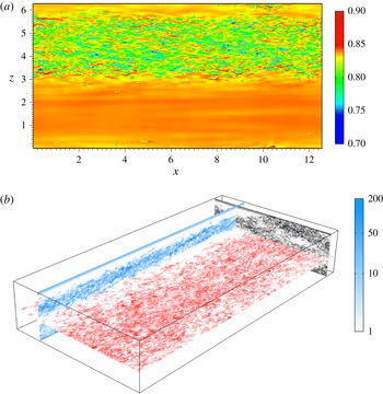
increases, the extent of the laminar regions increases and the dynamics becomes increasingly more intermittent in time. Figure 7(a) shows a snapshot of the streamwise velocity close to the upper wall, at
 $y=0.95$
, for simulation 14. There is only one band of turbulence spanning the entire streamwise extent, and this band is surrounded by laminar flow. As is apparent from the typical values of the streamwise velocity (the same colour bar is used in figures 6
c and 7
a), the streamwise velocity is substantially closer to its laminar value at
 $y=0.95$
for simulation 14 than for the more vigorously turbulent simulation 13. In this simulation,
 $\mathit{Re}_{{\it\tau}}$
varies considerably in time, ranging between 380 and 540, which suggests that the size of the computational domain is only marginally large enough to accommodate sustained intermittent dynamics. The topology found in figure 7 was similarly observed in simulations 15 and 16, confirming that also in these cases the computational domains were close to marginal.
Streamwise velocity in a horizontal plane close to the upper wall, at
 $y=0.95$
. It should be noted that the full domain is shown in each of the three cases, which vary in size. (a) Simulation 8; (b) simulation 10; (c) simulation 13.

Flow field for a highly intermittent simulation (simulation 14). The entire domain is shown in both panels. (a) Streamwise velocity in a horizontal plane close to the upper wall, at
 $y=0.95$
. The full domain is shown and colours range from blue (low values) to red (high values), using the same colour bar as figure 6(c). (b) Three-dimensional view of the enstrophy in three planes normal to the Cartesian axes:
 $x$
-normal at
 $x=12$
(black),
 $y$
-normal at
 $y=-0.2$
(red) and
 $z$
-normal at
 $z=1$
(blue). The scale logarithmically ranges from 1
 $U^{2}/h^{2}$
to 200
 $U^{2}/h^{2}$
and it is the same in all of the plots. Colours are used only to highlight which plane the contours belong to.

We only observe bands similar to those observed by Brethouwer et al. (Reference Brethouwer, Duguet and Schlatter2012) at low
 $\mathit{Re}_{{\it\tau}}<100$
, for which very large computational domains could be used. In smaller computational domains, the spatial intermittency is replaced by temporal intermittency and the turbulent bands align in the streamwise direction. However, the fact that at
 $\mathit{Re}_{{\it\tau}}=540$
we find streamwise stripes of turbulence similar to those found in low-
 $\mathit{Re}$
small-domain simulations suggests that inclined bands might be observed at higher
 $\mathit{Re}$
if larger computational domains were employed.
At low
 $\mathit{Re}$
, the laminar regions extend over the entire channel depth. However, we find that the vertical structure of the laminar/turbulent regions is inherently different for simulations at low and high
 $\mathit{Re}$
. As
 $\mathit{Ri}$
increases, laminar regions appearing at higher
 $\mathit{Re}$
become more confined to the walls. Brethouwer et al. (Reference Brethouwer, Duguet and Schlatter2012) found that in stratified channel flows partial relaminarisation occurs at the walls, whereas the dynamics in the interior remains highly turbulent, without any dominant presence of large-scale structures. In figure 7(b) the enstrophy (a useful and simple proxy for turbulence) in planes normal to the three Cartesian axis is shown for simulation 14. The contours projected onto the three Cartesian planes are coloured differently (although with the same intensity scale). The
 $z$
-normal plane clearly shows the presence of two turbulent layers separated by a quieter laminar region close to the channel mid-plane. This quieter region is confined horizontally and it is bordered in the spanwise direction by a turbulent patch which originates from the bending of the upper vertically confined turbulent layer, as shown by the
 $x$
-normal plane. Figure 7(b) highlights a rich dynamical picture in which intermittency at the wall connects to intermittent dynamics in the centre of the channel, with streamwise turbulent layers bending and mutually interacting. The dynamical transition between the turbulent bands (filling the entire channel gap) observed at low
 $\mathit{Re}$
and the layering structure in figure 7(b) is gradual. The bands moderately develop a spanwise inclination which leads to an inhomogeneity in the vertical direction.
It is unclear whether the absence of intermittent dynamics in the interior as observed by Brethouwer et al. (Reference Brethouwer, Duguet and Schlatter2012) is due to a weaker stratification or to a difference of flow configuration with respect to our simulations. It is nevertheless worth noting that in PCF intermittency at the wall significantly affects the overall dynamics. From an energetic point of view, PCF is forced by shear stresses at the upper and lower walls, and the dynamics in the interior adjusts in order to carry the momentum flux resulting from the near-wall dynamics. Full or partial relaminarisation leads to a significant drop in the magnitude of the wall shear stress
 ${\it\tau}_{w}$
, thus also strongly affecting the dynamics in the interior. The influence of the partial relaminarisation at the walls might therefore be significantly stronger than in other flow configurations where the driving force is not affected by relaminarisation, such as the channel flows considered by Brethouwer et al. (Reference Brethouwer, Duguet and Schlatter2012) driven by a constant pressure gradient or the throttling method used by Chung & Matheou (Reference Chung and Matheou2012) in stably stratified homogeneous turbulence.
4.2. Quantifying intermittency
One of our main aims here is to describe the intermittent regime arising due to a stable stratification. In order to quantify the degree of intermittency, an objective metric based on the identification of laminar and turbulent regions is needed. Several choices are possible, including evaluation of shear stress, vertical velocity (Brethouwer et al. Reference Brethouwer, Duguet and Schlatter2012) and vorticity (Corrsin & Kistler Reference Corrsin and Kistler1955; Pope Reference Pope2000).
We base our criterion on the wall enstrophy,
 $$\begin{eqnarray}{\it\eta}_{\pm }(x,z,t)=\left(\frac{\partial u}{\partial y}\right)^{2}+\left(\frac{\partial w}{\partial y}\right)^{2}\quad \text{at }y=\pm 1,\end{eqnarray}$$
and identify the turbulent fraction
 ${\it\gamma}$
using moments of the distribution of
 ${\it\eta}_{\pm }$
as discussed below. We are motivated to use the wall enstrophy by two considerations. First, as observed by Brethouwer et al. (Reference Brethouwer, Duguet and Schlatter2012), at large
 $\mathit{Re}$
when intermittent dynamics appears laminar patches are generally confined close to the walls. Second, as discussed in § 4.1, because the driving force is applied at the solid walls, near-wall dynamics plays an important role in maintaining turbulence in PCF. In order to identify
 ${\it\gamma}$
, we consider the horizontal spatial fluctuation of
 ${\it\eta}_{\pm }$
at the wall,
 $$\begin{eqnarray}{\it\eta}_{\pm ,mbf}=\sqrt{\frac{1}{A}\int _{x^{+},z^{+}}{\it\eta}_{\pm }^{2}\,\text{d}x^{+}\,\text{d}z^{+}-\left[\frac{1}{A}\int _{x^{+},z^{+}}{\it\eta}_{\pm }\,\text{d}x^{+}\,\text{d}z^{+}\right]^{2}},\end{eqnarray}$$
over subdomains corresponding to a minimal flow unit (Jiménez & Moin Reference Jiménez and Moin1991), specifically
 ${\rm\Delta}x^{+}\approx 200$
and
 ${\rm\Delta}z^{+}\approx 100$
, with
 $A={\rm\Delta}x^{+}\,{\rm\Delta}z^{+}$
being the subdomain area. The subscript
 $mbf$
in (4.2) stands for minimal box fluctuation. Although here we use
 ${\it\eta}_{\pm }$
as a proxy in (4.2), alternative quantities could also be used, such as velocity, temperature or turbulent stresses. When the flow is laminar, the wall enstrophy
 ${\it\eta}_{\pm }$
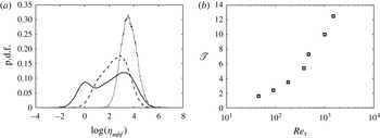
is nearly homogeneous within the subdomains and small values of (4.2) are to be expected. On the other hand, in turbulent regions the streaky patterns associated with the near-wall dynamics lead to significantly larger fluctuations. This measure is similar to the measure used by Deusebio et al. (Reference Deusebio, Brethouwer, Schlatter and Lindborg2014), although here there is a greater focus on identifying an appropriate threshold between laminar and turbulent regions. Figure 8(a) shows some examples of the probability density function (p.d.f.) of (4.2). The cases are characterised by different levels of intermittency: fully developed turbulence has a p.d.f. resembling a log-normal shape (the
 $x$
-axis has a logarithmic scale) with a single well-identified peak (Örlü & Schlatter Reference Örlü and Schlatter2011). As intermittent dynamics occurs in the flow, the p.d.f. skews towards the left part of the plot and, in sufficiently strongly intermittent cases, a double peak appears. The double-peak shape also allows us to identify a threshold
 $\mathscr{T}$
separating turbulent and laminar regions as the local minimum between the two peaks of the p.d.f. We identify laminar flow at the upper or lower wall as the region for which
 ${\it\eta}_{\pm ,mbf}<\mathscr{T}$
and turbulent flow as the region for which
 ${\it\eta}_{\pm ,mbf}>\mathscr{T}$
. In general, the threshold
 $\mathscr{T}$
may depend on
 $\mathit{Re}_{{\it\tau}}$
and we have determined its
 $\mathit{Re}_{{\it\tau}}$
dependence (shown in figure 8
b) by considering the most intermittent simulations at several values of
 $\mathit{Re}_{{\it\tau}}$
. Although the value of the threshold increases with
 $\mathit{Re}_{{\it\tau}}$
, it does not vary as strongly as the range spanned by the p.d.f., which in intermittent cases extends over several orders of magnitude. In the following we will consider the intermittency factor
 ${\it\gamma}$
for all of the simulations in table 1 by taking the average of the fraction of the upper and lower wall area for which
 ${\it\eta}_{\pm }>\mathscr{T}$
respectively. Typically, these two values are close. The algorithm described above was applied to single flow fields and results were averaged over at least 30 different sample times approximately equally spaced during the simulation.
(a) Examples of p.d.f.s of small-box fluctuations of
 ${\it\eta}_{\pm }$
for a typical fully turbulent simulation (
 $\cdots \cdots$
, simulation 9), weakly intermittent simulation (- - - -, simulation 10) and strongly intermittent simulation (——, simulation E). (b) Variation of
 $\mathscr{T}$
with
 $\mathit{Re}_{{\it\tau}}$
.

Although we mostly focus on the near-wall value of
 ${\it\gamma}$
, in order to study the mixing properties of laminar and turbulent regions separately (as discussed in § 5), we have further extended the algorithm to horizontal planes away from the wall using the total enstrophy in place of its wall value
 ${\it\eta}_{\pm }$
. To account for the vertical inhomogeneity, we have adjusted the value of the threshold
 $\mathscr{T}$
based on the local turbulent kinetic energy dissipation,
 ${\it\varepsilon}_{K}=\mathit{Re}^{-1}\langle \overline{\partial u_{i}^{\prime }/\partial x_{j}\partial u_{i}^{\prime }/\partial x_{j}}\rangle$
, as
 $$\begin{eqnarray}\mathscr{T}_{s}(y)=\frac{\mathscr{T}}{{\it\varepsilon}_{K,\pm 1}}{\it\varepsilon}_{K}(y),\end{eqnarray}$$
where the
 $\pm 1$
subscript denotes upper and lower wall values respectively. Using the threshold
 $\mathscr{T}_{s}$
, we define the vertically varying intermittency factor
 ${\it\gamma}_{s}$
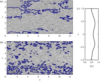
as the ratio of the turbulent area to the total area for each horizontal plane. Figure 9 shows an example of the identification of laminar/turbulent regions for the flow field shown in figure 6(c). Laminar and turbulent boundaries are well estimated, both close to the wall, as shown in figure 9(a) and in the centre of the channel, as shown in figure 9(b). The average value of
 ${\it\gamma}_{s}$
using roughly 30 flow fields (shown in figure 9
c) slightly varies in the vertical direction, with somewhat smaller values close to the wall, where an overall intermittency factor of 82 % is found. This is consistent with the observation of Brethouwer et al. (Reference Brethouwer, Duguet and Schlatter2012), who found laminar patches to be mostly confined at the wall. That the smallest value of
 ${\it\gamma}_{s}$
generally corresponds to the wall value
 ${\it\gamma}$
also supports our conjecture that the relaminarisation process in stratified PCF originates in the near-wall region.
Identification of laminar and turbulent regions using the automatic algorithm outlined in § 4.2 for a snapshot of simulation 13 at (a)
 $y=0.95$
and (b)
 $y=0$
. The thick line represents the boundary between laminar and turbulent regions which has been overlaid on the enstrophy field for reference. The flow corresponds to the same time instant as the flow depicted in figure 6(c) (simulation 13). (c) Wall-normal evolution of the intermittency factor
 ${\it\gamma}_{s}$
(averaged over roughly 30 snapshots).

4.3. Scaling of intermittent dynamics
As discussed in the introduction, the most appropriate indicator for the onset of intermittent dynamics is still an open issue and several criteria have been proposed. The general disagreement on the relevant quantity generally reflects the fact that it is not yet clear which physical process governs relaminarisation and how to model it. The Miles–Howard criterion (Howard Reference Howard1961; Miles Reference Miles1961), based on linear stability analysis of a stratified shear layer, is sometimes invoked to explain the suppression of turbulence, although there is now a growing consensus that turbulence may still be observed even when
 $\mathit{Ri}_{g}>1/4$
(see, for example, Zilitinkevich et al.
Reference Zilitinkevich, Elperin, Kleeorin, Rogachevskii, Esau, Mauritsen and Miles2008). As shown in figure 3(b),
 $\mathit{Ri}_{g}$
attains small values at the wall and increases towards the centreline, the location at which higher values are generally found. The maximum values of
 $\mathit{Ri}_{g}$
before the onset of intermittency and relaminarisation show an approximate dependence with bulk
 $\mathit{Ri}$
, and no single value describes the appearance of intermittency. Besides, intermittency is observed at the wall where
 $\mathit{Ri}_{g}$
is small,
 $\mathit{Ri}_{g}<1/4$
.
García-Villalba & del Álamo (Reference García-Villalba and del Álamo2011) used the Nusselt number
 $\mathit{Nu}$
, as defined in (2.10), as a criterion to identify the appearance of intermittency in stratified channel flows, arguing that relaminarisation occurs as
 $\mathit{Nu}$
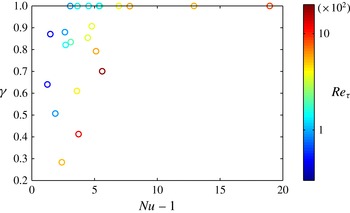
approaches unity. This criterion is tested in figure 10, where
 ${\it\gamma}$
is plotted against
 $\mathit{Nu}-1$
. Although as intermittency increases the data generally tend to lower values of
 $\mathit{Nu}$
, a general scaling cannot be observed and the data show a large scatter with
 $\mathit{Re}_{{\it\tau}}$
.
A plot of
 ${\it\gamma}$
versus
 $\mathit{Nu}-1$
for the entire set of simulations listed in table 1. The colour code represents
 $\mathit{Re}_{{\it\tau}}$
, ranging from 40 (blue) to 1500 (red).

As noted in the introduction, another criterion was proposed by Flores & Riley (Reference Flores and Riley2010), who hypothesised that relaminarisation is observed when
 $L^{+}\approx 100$
, thus suggesting that relaminarisation is a near-wall process since
 $L^{+}$
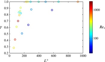
is a criterion only based on inner-scaling quantities. We test this hypothesis in figure 11, where the turbulent fraction
 ${\it\gamma}$
is plotted versus
 $L^{+}$
for all of the simulations listed in table 1. We note that, apart from the two lowest values of
 $\mathit{Re}_{{\it\tau}}$
(plotted with the four darkest blue points in the plot), the data collapse onto a single curve, unlike the data shown in figure 10. This is quite remarkable given the
 $\mathit{Re}_{{\it\tau}}$
span considered in the study, which covers more than one order of magnitude. The failure to collapse the two lowest values of
 $\mathit{Re}_{{\it\tau}}$
is also not surprising as the
 $L^{+}$
criterion is expected to apply only when the onset of intermittency is determined by the imposed stratification as opposed to by viscous effects. For smaller
 $\mathit{Re}$
values, viscosity becomes crucial and leads to a viscosity-driven intermittency, which in the unstratified limit occurs when
 $\mathit{Re}\approx 325$
, corresponding to
 $\mathit{Re}_{{\it\tau}}\approx 35$
. Nevertheless, the asymptotic regime in which intermittency dynamics is buoyancy-driven and the intermittency factor
 ${\it\gamma}$
becomes independent of
 $Re$
is already reached at a value of
 $\mathit{Re}_{{\it\tau}}$
that is only three times larger than the unstratified value of 35. As shown in figure 11, in the asymptotic regime of high
 $\mathit{Re}$
,
 $\mathit{Re}>4000$
, intermittent dynamics appears at
 $L^{+}\approx 200$
, and the intermittency factor
 ${\it\gamma}$
quickly drops for smaller values.
A plot of
 ${\it\gamma}$
versus
 $L^{+}$
for the entire set of simulations. The colour code represents
 $\mathit{Re}_{{\it\tau}}$
, ranging from 40 (blue) to 1500 (red).

5. Mixing
One of the most controversial issues regarding stably stratified shear flows concerns the quantification of the irreversible mixing across isopycnals and its ratio with the energy lost to internal energy through viscosity. At least part of the problem is that there are many possible measures that can be constructed for the ‘mixing efficiency’ (see, for example, Salehipour & Peltier Reference Salehipour and Peltier2015). In the context of shear flow, turbulent kinetic energy is typically extracted from the mean flow by the turbulence production term,
 $$\begin{eqnarray}P=\left\langle -\overline{u^{\prime }v^{\prime }}\frac{\partial \overline{u}}{\partial y}\right\rangle ,\end{eqnarray}$$
and undergoes a down-scale turbulent cascade until it is dissipated by viscous effects at small scales. In the presence of a stable stratification, turbulent kinetic energy can also be converted to potential energy (and vice versa) via the buoyancy flux,
 $$\begin{eqnarray}\mathscr{B}=\mathit{Ri}\,\langle -\overline{v^{\prime }T^{\prime }}\rangle .\end{eqnarray}$$
Similarly to turbulent kinetic energy, potential energy also generates a down-scale turbulence cascade, and diffusive effects convert it to background potential energy at small scales. A classical measure of the efficiency of mixing is the flux Richardson number (see, e.g., Turner Reference Turner1979),
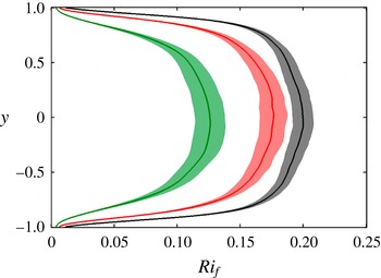
 $$\begin{eqnarray}\mathit{Ri}_{f}(y)=\frac{\mathit{Ri}\,\langle -\overline{v^{\prime }T^{\prime }}\rangle }{\displaystyle \left\langle -\overline{u^{\prime }v^{\prime }}\frac{\partial \overline{u}}{\partial y}\right\rangle },\end{eqnarray}$$
representing the ratio between the buoyancy flux
 $\mathscr{B}$
and the turbulence production
 $P$
. Figure 12 shows the
 $\mathit{Ri}_{f}(y)$
profiles for simulations 9, 11 and 13. The bands around the solid lines represent the standard deviation of
 $\mathit{Ri}_{f}$
calculated from the time variation of
 $\mathit{Ri}_{f}$
. It can be seen that
 $\mathit{Ri}_{f}(y)$
shows a very similar behaviour to
 $\mathit{Ri}_{g}$
, with low values at the wall and a rather broad maximum at the centre, even though the values of
 $\mathit{Ri}_{f}$
are slightly larger. This indicates that for the simulations considered here the turbulent Prandtl number
 $\mathit{Pr}_{T}=\mathit{Ri}/\mathit{Ri}_{f}={\it\nu}_{T}/{\it\kappa}_{T}$
is slightly smaller than unity, where
 ${\it\nu}_{T}$
and
 ${\it\kappa}_{T}$
are the eddy viscosity and the eddy diffusivity respectively. Fluctuations around mean values are significantly stronger at the centre and rapidly reduce near the walls. Thus,
 $\mathit{Ri}_{f}(y)$
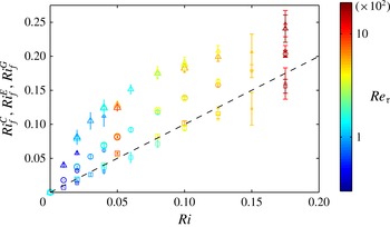
is a spatially varying local measure of the mixing efficiency. In figure 13, we compare two different derived measures of
 $\mathit{Ri}_{f}$
. The triangles represent values of
 $\mathit{Ri}_{f}^{C}$
, i.e.
 $\mathit{Ri}_{f}(y)$
averaged locally at the centre of the channel
 $0.1<y<-0.1$
, and the circles represent values of
 $\mathit{Ri}_{f}^{E}$
, i.e.
 $\mathit{Ri}_{f}(y)$
averaged globally across the entire channel
 $-1<y<+1$
. Because of the lower values of
 $\mathit{Ri}_{f}$
observed at the wall,
 $\mathit{Ri}_{f}^{C}$
is larger than
 $\mathit{Ri}_{f}^{E}$
. Nevertheless, both sets of data show a clear increase with
 $\mathit{Ri}$
and a tendency to saturate for large values. Unfortunately, the relatively small
 $\mathit{Re}$
did not allow us to obtain turbulent states for
 $\mathit{Ri}>0.175$
, where the behaviour of
 $\mathit{Ri}_{f}$
is most debated and non-monotonic dependence in
 $\mathit{Ri}$
is sometimes seen in experiments (see, e.g., Linden Reference Linden1979; Park et al.
Reference Park, Whitehead and Gnanadeskian1994; Holford & Linden Reference Holford and Linden1999; Oglethorpe et al.
Reference Oglethorpe, Caulfield and Woods2013).
Vertical variation of
 $\mathit{Ri}_{f}(y)$
, as defined in (5.3). The shaded regions represent the
 $\pm {\it\sigma}$
intervals, where
 ${\it\sigma}$
is the standard deviation. Lines: left, simulation 9; middle, simulation 11; right, simulation 13.

Comparison of different measures of
 $\mathit{Ri}_{f}$
for the simulations listed in table 1. The symbols represent (▵)
 $\mathit{Ri}_{f}^{C}$
, derived from
 $\mathit{Ri}_{f}(y)$
vertically averaged in the centre
 $-0.1<y<0.1$
, (○)
 $\mathit{Ri}_{f}^{E}$
, derived from
 $\mathit{Ri}_{f}(y)$
averaged over the entire channel
 $-1<y<1$
, and (▫)
 $\mathit{Ri}_{f}^{G}$
given by (5.9). The error bar corresponds to
 $\pm {\it\sigma}$
, where
 ${\it\sigma}$
represents the standard deviation of time varying quantities. The dashed black thin line represents the bisect, i.e.
 $\mathit{Ri}_{f}=\mathit{Ri}$
. Data markers are colour-coded proportional to the simulation value of
 $\log _{10}\mathit{Re}_{{\it\tau}}$
, ranging from 40 (blue) to 1500 (red), with the size of the markers proportional to the turbulent fraction
 ${\it\gamma}$
.

The simplified wall-bounded nature of stratified PCF also allows us to identify another global measure of mixing in terms of properties of the wall forcing. By integrating the kinetic energy and the potential energy, defined as
 $-\mathit{Ri}\int Ty\,\text{d}V$
, over the whole domain, we can derive an evolution equation for the total energy of the system:
 $$\begin{eqnarray}\frac{\text{d}E_{TOT}}{\text{d}t}=2{\it\tau}_{w}-\int _{-1}^{+1}({\it\varepsilon}_{M}+{\it\varepsilon}_{K}+{\it\varepsilon}_{P})\,\text{d}y,\end{eqnarray}$$
where
 $2{\it\tau}_{w}$
represents the forcing due to the counter-moving walls and the
 ${\it\varepsilon}_{i}$
terms represent the dissipation of mean kinetic energy,
 $$\begin{eqnarray}{\it\varepsilon}_{M}=\frac{1}{\mathit{Re}}\left\langle \frac{\partial \overline{u}}{\partial x_{j}}\frac{\partial \overline{u}}{\partial x_{j}}\right\rangle ,\end{eqnarray}$$
turbulent kinetic energy,
 $$\begin{eqnarray}{\it\varepsilon}_{K}=\frac{1}{\mathit{Re}}\left\langle \overline{\frac{\partial u_{i}^{\prime }}{\partial x_{j}}\frac{\partial u_{i}^{\prime }}{\partial x_{j}}}\right\rangle ,\end{eqnarray}$$
and potential energy,
 $$\begin{eqnarray}{\it\varepsilon}_{P}=\frac{1}{\mathit{Re}\,\mathit{Pr}}\left\langle \overline{\frac{\partial \tilde{T}}{\partial x_{j}}\frac{\partial \tilde{T}}{\partial x_{j}}}\right\rangle ,\end{eqnarray}$$
where
 $u^{\prime }$
is the velocity fluctuation around the mean and
 $\tilde{T}$
is the temperature fluctuation around a linear stratification. In a statistically steady state, equation (5.4) can be reduced to the dimensionless form
 $$\begin{eqnarray}1-\mathit{Ri}_{f}^{G}=(\tilde{{\it\varepsilon}}_{M}+\tilde{{\it\varepsilon}}_{K})\frac{\mathit{Re}^{2}}{\mathit{Re}_{{\it\tau}}^{2}},\end{eqnarray}$$
where
 $\tilde{{\it\varepsilon}}_{M}$
is the
 $y$
-integrated mean kinetic energy dissipation and
 $\tilde{{\it\varepsilon}}_{K}$
is the integrated turbulent kinetic energy dissipation. Thus,
 $\mathit{Ri}_{f}^{G}$
is a global measure of the mixing,
 $$\begin{eqnarray}\mathit{Ri}_{f}^{G}=\frac{\mathit{Ri}\,\mathit{Re}\,(\mathit{Nu}-1)}{\mathit{Re}_{{\it\tau}}^{2}\,\mathit{Pr}},\end{eqnarray}$$
and we also plot this measure in figure 13 with squares. It is seen that
 $\mathit{Ri}_{f}^{G}$
attains smaller values than
 $\mathit{Ri}_{f}$
, due to the fact that
 $\mathit{Ri}_{f}^{G}$
also includes contributions of mean kinetic energy dissipation in the denominator, which is large near the wall. This effect can be identified directly by rewriting
 $\mathit{Ri}_{f}^{G}$
as
 $$\begin{eqnarray}\mathit{Ri}_{f}^{G}=\frac{\displaystyle -\mathit{Ri}\int \langle \overline{v^{\prime }T^{\prime }}\rangle \,\text{d}y}{\displaystyle \int \left\langle \frac{\partial }{\partial y}\left[\left(\frac{1}{\mathit{Re}}\frac{\partial \overline{u}}{\partial y}-\overline{u^{\prime }v^{\prime }}\right)\overline{u}\right]\right\rangle \,\text{d}y}=\frac{\displaystyle -\mathit{Ri}\int \langle \overline{v^{\prime }T^{\prime }}\rangle \,\text{d}y}{\displaystyle \int \langle \tilde{{\it\varepsilon}}_{M}\rangle \,\text{d}y-\int \left\langle \overline{u^{\prime }v^{\prime }}\frac{\partial \overline{u}}{\partial y}\right\rangle \,\text{d}y},\end{eqnarray}$$
where the fact that the total shear
 ${\it\nu}\partial \overline{u}/\partial y-\overline{u^{\prime }v^{\prime }}$
is constant has been used. Equation (5.10) indicates that reductions relative to
 $\mathit{Ri}_{f}^{C}$
and
 $\mathit{Ri}_{f}^{E}$
arise as a consequence of mean kinetic energy dissipation (first term in the denominator), which is large close to the walls.
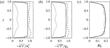
Comparison between the conditional average based on turbulent regions (- - - -) and the conditional average based on laminar regions (
 $\cdots \cdots$
) for simulation 13. Conditional values are obtained by averaging the horizontally averaged values over roughly 30 snapshots. The non-conditional values (——) obtained by averaging in time, i.e.
 $\langle \cdot \rangle$
, are also shown for reference. Vertical variation of (a) turbulent shear stress
 $-\overline{u^{\prime }v^{\prime }}/u_{{\it\tau}}^{2}$
, (b) turbulent heat flux
 $-\overline{v^{\prime }T^{\prime }}/q_{w}$
and (c) flux Richardson number
 $\mathit{Ri}_{f}$
as defined in (5.3).

The
 $\mathit{Ri}_{f}^{G}$
data points approximately follow a straight line corresponding to
 $\mathit{Ri}_{f}^{G}=\mathit{Ri}$
, suggesting that velocity and temperature are closely related and show very similar behaviour such that
 $q_{w}\approx {\it\tau}_{w}$
. This is consistent with the finding of Cenedese & Adduce (Reference Cenedese and Adduce2008) and Wells, Cenedese & Caulfield (Reference Wells, Cenedese and Caulfield2010), who suggest a scaling of the mixing efficiency at ‘weak’ stratification proportional to the inverse square of an appropriate Froude number, which here is equivalent to the first power of the bulk Richardson number,
 $Fr^{-2}\sim \mathit{Ri}$
. It is apparent that simulations at large
 $\mathit{Re}$
and
 $\mathit{Ri}$
generally show a somewhat larger degree of fluctuations of
 $\mathit{Ri}_{f}^{G}$
. In particular, simulation 14 exhibits the largest variance, possibly due to the strong degree of intermittency found in this case. In order to investigate to what extent
 $\mathit{Ri}_{f}$
depends on the global intermittency of the flow, the size of the symbols in figure 13 has been modified to reflect the value of
 ${\it\gamma}$
. Surprisingly, the dependence of
 $\mathit{Ri}_{f}$
on
 ${\it\gamma}$
is relatively small. To understand better how laminar and turbulent regions contribute to the total mixing separately, we have calculated the turbulent shear stresses
 $-\overline{u^{\prime }v^{\prime }}$
, the turbulent heat fluxes
 $-\overline{v^{\prime }T^{\prime }}$
and the flux Richardson number
 $\mathit{Ri}_{f}$
in laminar and turbulent regions separately for a number of flow fields (approximately 30) of simulation 13 and averaged their values (figure 14). Fluctuations have been computed using averages applied in laminar regions and turbulent regions separately in order to avoid spurious fluctuations due to the variation of mean profiles in laminar and turbulent regions. In laminar regions, velocity and temperature fluctuations are greatly reduced with respect to their turbulent counterparts. The magnitudes of
 $\overline{u^{\prime }v^{\prime }}$
and
 $\overline{v^{\prime }T^{\prime }}$
in laminar regions drop to approximately 20–25 % of the equivalent magnitude in turbulent regions. Nevertheless, despite this reduction,
 $\mathit{Ri}_{f}$
does not significantly change, indicating that
 $\overline{u^{\prime }v^{\prime }}$
and
 $\overline{v^{\prime }T^{\prime }}$
decrease proportionately such that their ratio remains close to constant. This highlights once more the close relationship between the velocity and the temperature fields. Momentum fluxes and heat fluxes both originate from the vertical advection of mean velocity and mean temperature gradients, and they reduce in the same manner as the vertical velocity fluctuation drops. This is an unexpected result as it is typically argued that more quiescent (i.e. laminar) regions should be associated with smaller mixing efficiencies since the surviving waves can still transport energy but not heat. It is important to remember that the regions that we refer to as ‘laminar’ are in fact constantly deformed and convected by the surrounding turbulence, still retaining 20–25 % of the turbulent fluctuations. This, together with the imposed mean velocity gradients, generates momentum and heat fluxes associated with
 $\mathit{Ri}_{f}$
similar to the ones found in turbulent regions.
An understanding of how the efficiency of mixing varies as a function of
 $\mathit{Re}$
and
 $\mathit{Ri}$
is one of the most important problems in stratified turbulent dynamics and is certainly of central importance for parametrisation of mixing in large-scale models (see Ivey, Winters & Koseff Reference Ivey, Winters and Koseff2008). We have attempted to unravel the shape of the
 $\mathit{Ri}_{f}=f(\log _{10}\mathit{Re},\mathit{Ri})$
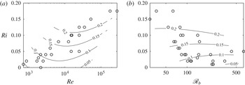
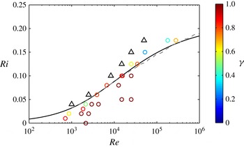
surface by finding the surface that best approximates our observations. In appendix A, we outline the interpolation method in more detail. The contour levels of
 $\mathit{Ri}_{f}$
, shown in figure 15(a), display a weak non-monotonic behaviour in
 $\mathit{Re}$
with the presence of a local maximum close to the region where intermittency appears. It would be interesting to explore whether this reduction of
 $\mathit{Ri}_{f}$
observed at large
 $\mathit{Re}$
is real or is an artefact of the interpolation. Unfortunately, this regime is currently inaccessible due to the large computational cost associated with large
 $\mathit{Re}_{{\it\tau}}$
. In order to frame our results in the light of the recent advances in the understanding of stratified turbulence (e.g. Billant & Chomaz Reference Billant and Chomaz2001; Lindborg Reference Lindborg2006; Brethouwer et al.
Reference Brethouwer, Billant, Lindborg and Chomaz2007), figure 15 shows the
 $\mathit{Ri}_{f}$
surface in a plane where
 $\mathit{Re}$
has been replaced by the buoyancy Reynolds number (Brethouwer et al.
Reference Brethouwer, Billant, Lindborg and Chomaz2007),
 $$\begin{eqnarray}\mathscr{R}_{b}=\frac{{\it\varepsilon}_{K}\,\mathit{Re}}{\mathit{Ri}}.\end{eqnarray}$$
On the
 $\mathscr{R}_{b}{-}\mathit{Ri}$
plane, the variation of
 $\mathit{Ri}_{f}$
is somewhat smoothed and
 $\mathit{Ri}_{f}$
is approximately constant with
 $\mathscr{R}_{b}$
, with
 $\mathscr{R}_{b}$
in the range between 30 and 650. Figure 15(b) also shows the intrinsic limitations and difficulties of simulating stratified turbulent flows. Because of the reduction of vertical length scale due to a stable stratification,
 $\mathscr{R}_{b}$
decreases as we move towards the top right corner of figure 2(a), corresponding to larger values of both
 $\mathit{Re}$
and
 $\mathit{Ri}$
.
Interpolated surface of
 $\mathit{Ri}_{f}$
on (a) an
 $\mathit{Re}{-}\mathit{Ri}$
and (b) an
 $\mathscr{R}_{b}{-}\mathit{Ri}$
plane. The symbols mark the values for the simulations in table 1.

6. Models for predicting the intermittency boundary
The
 $L^{+}$
criterion (i.e.
 $L^{+}\leqslant 200$
) tested in figure 11 can be particularly useful to predict where the boundary separating intermittent and turbulent dynamics lies in the
 $\mathit{Re}{-}\mathit{Ri}$
plane. In order to construct this prediction, we rewrite
 $L^{+}$
as
 $$\begin{eqnarray}L^{+}=\frac{\mathit{Re}_{{\it\tau}}^{4}\,\mathit{Pr}}{C_{{\it\kappa}}\,\mathit{Re}^{2}\,\mathit{Ri}\,\mathit{Nu}}.\end{eqnarray}$$
Since throughout our simulations
 $\mathit{Pr}$
is held fixed, modelling of the functional dependence of
 $L^{+}$
on the externally fixed parameters
 $\mathit{Re}$
and
 $\mathit{Ri}$
is equivalent to constructing models for the dependence of
 $\mathit{Re}_{{\it\tau}}$
and
 $\mathit{Nu}$
on
 $\mathit{Re}$
and
 $\mathit{Ri}$
. In the following, we compare two such models: one simple analytical model and a more complex Reynolds-averaged Navier–Stokes (RANS) model, which potentially provides an increasing degree of accuracy at the expense of simplicity.
6.1. Monin–Obukhov self-similarity theory
The analytical model is derived from the self-similarity theory proposed by Obukhov (Reference Obukhov1971) and Monin & Obukhov (Reference Monin and Obukhov1954). It provides analytical expressions for velocity and temperature profiles in unstable and stable stratifications. More generally, turbulent statistical moments are assumed to depend only on the vertical momentum transfer
 $-\overline{u^{\prime }v^{\prime }}$
(at first approximation equal to the wall shear stress
 ${\it\tau}_{w}$
), the buoyancy parameter
 $g{\it\alpha}_{V}$
, the height from the surface
 $y$
and the turbulent heat flux
 $-\overline{v^{\prime }T^{\prime }}$
(at first approximation equal to the wall heat flux
 $q_{w}$
). Dimensional analysis therefore leads to only one independent dimensionless group, suggesting that any statistical quantity, when properly normalised, is only a function of such a group, which could be (arbitrarily) identified by
 $$\begin{eqnarray}{\bf\xi}=\frac{y}{L},\end{eqnarray}$$
where
 $L$
is the Monin–Obukhov length scale, as defined in (2.11). In particular, the mean velocity and temperature gradients (dimensional) can therefore be written as
 $$\begin{eqnarray}\frac{\partial u}{\partial y}=\frac{u_{{\it\tau}}}{C_{{\it\kappa}}y}{\it\phi}_{m}({\bf\xi})\quad \text{and}\quad \frac{\partial T}{\partial y}=\frac{T_{{\it\tau}}}{C_{{\it\kappa}}y}{\it\phi}_{h}({\bf\xi}),\end{eqnarray}$$
where
 ${\it\phi}_{m}$
and
 ${\it\phi}_{h}$
are dimensionless functions, the von Kármán coefficient,
 $C_{{\it\kappa}}$
, is historically included in the definitions and
 $T_{{\it\tau}}$
is the friction temperature, i.e.
 $T_{{\it\tau}}=q_{w}/u_{{\it\tau}}$
. At first approximation,
 ${\it\phi}_{m}$
and
 ${\it\phi}_{h}$
are assumed to be linear functions of
 ${\bf\xi}$
, i.e.
 $$\begin{eqnarray}{\it\phi}_{m}({\bf\xi})=1+{\it\beta}{\bf\xi}\quad \text{and}\quad {\it\phi}_{m}({\bf\xi})=\mathit{Pr}_{T}+{\it\beta}{\bf\xi},\end{eqnarray}$$
with
 $\mathit{Pr}_{T}$
being the turbulent Prandtl number and
 ${\it\beta}$
a dimensionless constant. Despite its simplicity, Monin–Obukhov self-similarity theory has been successfully compared with in situ field measurements (Businger et al.
Reference Businger, Wyngaard, Izumi and Bradley1971; Kaimal et al.
Reference Kaimal, Wyngaard, Haugen, Coté, Izumi, Caughey and Readings1976) and numerical simulations (García-Villalba & del Álamo Reference García-Villalba and del Álamo2011; Ansorge & Mellado Reference Ansorge and Mellado2014; Deusebio et al.
Reference Deusebio, Brethouwer, Schlatter and Lindborg2014). In the following we develop a model based on it. By integrating the mean gradients given by (6.3) together with definitions (6.4), we arrive at an expression for the velocity and buoyancy jumps between the upper and lower walls,
 $$\begin{eqnarray}U=2\frac{u_{{\it\tau}}}{C_{{\it\kappa}}}\left(\log \mathit{Re}_{{\it\tau}}+{\it\beta}\frac{h}{L}+C_{{\it\kappa}}C_{1}\right)\end{eqnarray}$$
and
 $$\begin{eqnarray}T=2\frac{T_{{\it\tau}}}{C_{{\it\kappa}}}\left(\mathit{Pr}_{T}\log \mathit{Re}_{{\it\tau}}+{\it\beta}\frac{h}{L}+C_{{\it\kappa}}C_{2}\right),\end{eqnarray}$$
with
 $C_{1}$
and
 $C_{2}$
being constants. We note that Monin–Obukhov theory assumes a very similar shape for the velocity and temperature mean profiles, consistently with our simulations, as shown by the empirically observed scaling
 $\mathit{Ri}_{f}^{G}\sim \mathit{Ri}$
. Equations (6.5) and (6.6) can be rearranged to provide expressions relating
 $\mathit{Re}_{{\it\tau}}$
,
 $\mathit{Re}$
,
 $L$
and
 $\mathit{Ri}$
, i.e.
 $$\begin{eqnarray}\mathit{Re}=\frac{\mathit{Re}_{{\it\tau}}}{C_{{\it\kappa}}}\left(\log \mathit{Re}_{{\it\tau}}+{\it\beta}\frac{\mathit{Re}_{{\it\tau}}}{L^{+}}+C_{1}\right)\end{eqnarray}$$
and
 $$\begin{eqnarray}\mathit{Ri}=\frac{h}{L}\frac{\displaystyle \mathit{Pr}_{T}\log \mathit{Re}_{{\it\tau}}+{\it\beta}\frac{\mathit{Re}_{{\it\tau}}}{L^{+}}+C_{2}}{\left(\log \mathit{Re}_{{\it\tau}}+{\it\beta}{\displaystyle \frac{\mathit{Re}_{{\it\tau}}}{L^{+}}}+C_{1}\right)^{2}},\end{eqnarray}$$
from which the value of
 $L^{+}$
can be estimated. Here, we set
 ${\it\beta}=4.8$
,
 $\mathit{Pr}_{T}=0.7$
and
 $C_{1}=C_{2}=5.5$
in (6.7) and (6.8), similar to the values suggested by Wyngaard (Reference Wyngaard2010) and consistent with our simulations, indicating a
 $\mathit{Pr}_{T}$
slightly smaller than unity.
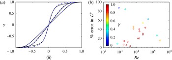
Figure 16(a) shows a comparison between the velocity profiles from the numerical simulations (already presented in figure 3) and the predictions provided by the Monin–Obukhov theory. Despite its simplicity, we observe a reasonable agreement, particularly in the core region of the flow. On the other hand, the agreement close to the walls is less good (especially for the unstratified simulation 6 for which
 $\mathit{Re}$
may well be too small to allow the development of a proper logarithmic layer), resulting in an error in the prediction of
 $\mathit{Re}_{{\it\tau}}$
and
 $L^{+}$
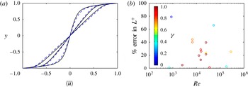
. In figure 16(b) we plot the percentage error difference,
 $$\begin{eqnarray}\frac{|L_{DNS}^{+}-L_{M}^{+}|}{L_{DNS}^{+}}\,\%,\end{eqnarray}$$
between the value obtained from the numerical simulations,
 $L_{DNS}^{+}$
, and the estimated value of the model using (6.7) and (6.8),
 $L_{M}^{+}$
. It is worth noting that the error in the prediction of
 $L^{+}$
tends to be larger when intermittency appears in the flow. In fully developed turbulent regimes the predicted value of
 $L^{+}$
is within a relative error of 20–40 %, which we believe is acceptable.
(a) Comparison between numerical simulations (——) and the analytical model (- - - -) defined in (6.5) and (6.6). The three profiles correspond to
 $\langle \overline{u}\rangle$
velocity profiles for the simulations 6, 11 and 13, shown in figure 3. (b) Percentage errors in the estimation of
 $L^{+}$
using the Monin–Obukhov model, as defined in (6.9). The symbols represent all of the simulations given in table 1 and are coloured by the turbulent fraction
 ${\it\gamma}$
, ranging from blue (laminar) to red (fully turbulent).

6.2. Explicit algebraic models
The more complex model we consider here is an EAM for turbulent Reynolds stresses and heat fluxes for stably stratified flows. An EAM is generally developed from differential Reynolds-stress models (DRSMs) in which the evolution equations for the Reynolds stresses and heat fluxes take the form (Pope Reference Pope2000)
 $$\begin{eqnarray}\frac{\text{D}\overline{u_{i}u_{j}}}{\text{D}t}-\mathscr{D}_{ij}=\mathscr{P}_{ij}+{\it\Pi}_{ij}-{\it\varepsilon}_{ij}+\mathscr{G}_{ij}\end{eqnarray}$$
and
 $$\begin{eqnarray}\frac{\text{D}\overline{u_{i}{\it\theta}}}{\text{D}t}-\mathscr{D}_{{\it\theta}i}=\mathscr{P}_{{\it\theta}i}+{\it\Pi}_{{\it\theta}i}-{\it\varepsilon}_{{\it\theta}i}+\mathscr{G}_{{\it\theta}i},\end{eqnarray}$$
where the terms correspond to (from left to right) advection, diffusion, production, pressure redistributions, dissipation and buoyancy. Following Lazeroms et al. (Reference Lazeroms, Brethouwer, Wallin and Johansson2013), equations (6.10) and (6.11) can be recast as evolution equations for the dimensionless counterparts
 $\unicode[STIX]{x1D622}_{ij}=\overline{u_{i}u_{j}}/K-2/3{\it\delta}_{ij}$
and
 ${\it\xi}_{i}=\overline{u_{i}{\it\theta}}/\sqrt{K\,K_{{\it\theta}}}$
, where
 $K$
is the turbulent kinetic energy,
 $\overline{u_{i}u_{i}}/2$
, and
 $K_{{\it\theta}}$
is the scalar variance,
 $\overline{{\it\theta}^{2}}/2$
. In EAMs, the weak-equilibrium assumption (Rodi Reference Rodi1976) is generally made at this stage, neglecting advection and diffusion terms in the evolution equations for
 $\unicode[STIX]{x1D622}_{ij}$
and
 ${\it\xi}_{i}$
. This allows one to reduce these equations to an algebraic form in which time derivatives and higher-order spatial derivatives of Reynolds stresses disappear, i.e.
 $$\begin{eqnarray}\frac{\overline{u_{i}u_{j}}}{K}(\mathscr{P}-{\it\varepsilon}+\mathscr{G})=\mathscr{P}_{ij}+{\it\Pi}_{ij}-{\it\varepsilon}_{ij}+\mathscr{G}_{ij}\end{eqnarray}$$
and
 $$\begin{eqnarray}\frac{\overline{u_{i}{\it\theta}}}{2}\left(\frac{\mathscr{P}-{\it\varepsilon}+\mathscr{G}}{K}+\frac{\mathscr{P}_{{\it\theta}}-{\it\varepsilon}_{{\it\theta}}}{K_{{\it\theta}}}\right)=\mathscr{P}_{i{\it\theta}}+{\it\Pi}_{i{\it\theta}}-{\it\varepsilon}_{i{\it\theta}}+\mathscr{G}_{ij}.\end{eqnarray}$$
In (6.12) and (6.13), the terms
 ${\it\Pi}_{ij}$
and
 ${\it\Pi}_{i{\it\theta}}-{\it\varepsilon}_{i{\it\theta}}$
can be modelled following Launder (Reference Launder1975), with expressions involving
 $K$
,
 $K_{{\it\theta}}$
and the other variables, i.e.
 $U_{i}$
,
 $T$
,
 $\unicode[STIX]{x1D622}_{ij}$
and
 ${\it\xi}_{i}$
. The dissipation term
 ${\it\varepsilon}_{ij}$
is assumed to be isotropic, i.e.
 ${\it\varepsilon}_{ij}=(2/3){\it\varepsilon}{\it\delta}_{ij}$
, where
 ${\it\varepsilon}$
is the turbulent kinetic energy dissipation. Equations (6.12) and (6.13) are implicit in
 $\unicode[STIX]{x1D622}_{ij}$
and
 ${\bf\xi}$
and highly nonlinear. However, explicit algebraic equations relating
 $\unicode[STIX]{x1D622}_{ij}$
and
 ${\bf\xi}$
to the other mean quantities can be derived by expanding
 $\unicode[STIX]{x1D622}_{ij}$
and
 ${\bf\xi}$
in tensor groups (Pope Reference Pope1975) and using an approximate equation for the kinetic energy production-to-dissipation ratio (Lazeroms et al.
Reference Lazeroms, Brethouwer, Wallin and Johansson2015). These relations together with suitable expressions for
 $K$
,
 $K_{{\it\theta}}$
and
 ${\it\varepsilon}$
such as the
 $K{-}{\it\omega}$
model (Menter Reference Menter1992) form a closed set of equations which can be numerically solved in time. For further details on the derivation of the model we refer the interested reader to Lazeroms et al. (Reference Lazeroms, Brethouwer, Wallin and Johansson2013, Reference Lazeroms, Brethouwer, Wallin and Johansson2015).
Explicit algebraic models have been successfully applied to stably stratified shear parallel flows and stably stratified channel flows, and provide fair agreement with simulations and significant improvements with respect to standard eddy-viscosity and eddy-diffusivity models (Lazeroms et al.
Reference Lazeroms, Brethouwer, Wallin and Johansson2013). In the following, we extend this comparison to PCF. It is worth emphasising here that all of the modelling constants are the same as in Lazeroms et al. (Reference Lazeroms, Brethouwer, Wallin and Johansson2013). The velocity (figure 17
a) and density profiles (not shown) agree reasonably well with the numerical simulations over the entire channel depth. Figure 17(b) shows the percentage error, as defined in (6.9) using EAMs for estimating the model value
 $L_{M}^{+}$
. The agreement is somewhat poor at low
 $\mathit{Re}$
but improves for increasing
 $\mathit{Re}$
, providing good predictions for
 $\mathit{Re}>5\times 10^{3}$
. That models and simulations do not agree at low
 $\mathit{Re}<5\times 10^{3}$
is not surprising since at such low
 $\mathit{Re}$
diffusive effects may well be important and the weak-equilibrium assumption may be inappropriate. Nevertheless, as long as
 $\mathit{Re}$
is large enough, the relative errors for estimating
 $\mathit{Re}_{{\it\tau}}$
and
 $L^{+}$
are approximately
 $10\,\%$
and
 $20\,\%$
respectively, slightly better than for the Monin–Obukhov self-similarity theory.
(a) Comparison between numerical simulations (——) and the EAM (- - - -) from Lazeroms et al. (Reference Lazeroms, Brethouwer, Wallin and Johansson2013). The three profiles correspond to
 $\langle \overline{u}\rangle$
for the simulations 6, 11 and 13, shown in figure 3. (b) Percentage errors in the estimation of
 $L^{+}$
using the analytical model. The symbols represent the simulations given in table 1 and are coloured by the turbulent fraction
 ${\it\gamma}$
, ranging from blue (laminar) to red (fully turbulent).

6.3. The intermittency boundary
We now use the models outlined in §§ 6.1 and 6.2 to predict the intermittency boundary in the
 $\mathit{Re}{-}\mathit{Ri}$
plane between turbulent and intermittent dynamics. According to figure 11, we predict that intermittency onsets at
 $L^{+}\approx 200$
. Using the two models, we have estimated
 $L^{+}$
as a function of
 $\mathit{Re}$
and
 $\mathit{Ri}$
, with
 $\mathit{Re}$
between 103 and 106 and
 $\mathit{Ri}$
between 0 and 0.2. A summary of the simulations together with the intermittency boundaries predicted by the two models is shown in figure 18. The colours represent the turbulent fraction
 ${\it\gamma}$
. The two models show an overall similar behaviour, and they are indistinguishable for most of the
 $\mathit{Re}$
range. Remarkably, the model based on the Monin–Obukhov self-similarity theory is able to provide good agreement with the numerical simulations and with the more complex EAM. It is nevertheless worth noting that PCF is a simple and idealised geometry in which, in statistically steady states, momentum and heat fluxes are constant across the channel. Analytical models may provide somewhat poorer performance in more complex flow geometries, where more refined models, such as EAM, have already been shown to provide better results. As shown in figure 18, at least at smaller
 $\mathit{Re}$
and
 $\mathit{Ri}$
, the intermittency and relaminarisation boundaries are quite close. It is still an open question whether this observation carries over to larger values of
 $\mathit{Re}$
and
 $\mathit{Ri}$
, particularly in sufficiently large computational domains.
Summary of the direct numerical simulations (circles) and predictions of the intermittency boundary given by the Monin–Obukhov theory (solid black line) and the EAM (dashed grey line). The symbols are coloured by the turbulent fraction
 ${\it\gamma}$
, ranging from blue (laminar) to red (fully turbulent). Triangles representing simulations that fully relaminarised are also shown for reference.

7. Conclusions
We have studied the onset of global intermittency in stably stratified PCFs using numerical simulations, in an attempt to identify the intermittency boundary depicted schematically by the solid line in figure 1. We have explored the flow dynamics for a number of
 $\mathit{Re}{-}\mathit{Ri}$
values, ranging from low
 $\mathit{Re}\sim 700$
(close to providing intermittent dynamics in unstratified conditions) to high
 $\mathit{Re}\sim 2.8\times 10^{5}$
. The
 $\mathit{Ri}$
at which intermittency arises increases with
 $\mathit{Re}$
, and no turbulent states have been found for
 $\mathit{Ri}\geqslant 0.2$
for the
 $\mathit{Re}$
considered here. At the largest
 $\mathit{Re}$
we have considered,
 $\mathit{Re}=2.8\times 10^{5}$
, a value of
 $\mathit{Ri}=0.175$
already leads to intermittency, with a significant portion of the flow being laminar.
Intermittency first appears in the form of laminar spots which grow and decay within the flow. As
 $\mathit{Ri}$
increases, these regions grow larger and turbulent bands span the entire domain, similar to the behaviour reported by Brethouwer et al. (Reference Brethouwer, Duguet and Schlatter2012). The dynamics of the laminar/turbulent patches show remarkably different features depending on
 $\mathit{Re}$
. At low
 $\mathit{Re}$
, viscously driven intermittency is characterised by laminar and turbulent regions which fill the entire channel gap and align horizontally along inclined bands, similar to the behaviour that has been previously reported in unstratified PCF. On the other hand, at high
 $\mathit{Re}$
and
 $\mathit{Ri}$
, buoyancy-driven intermittency leads to inhomogeneity in the vertical direction with an interplay of turbulent and laminar layers. At high
 $\mathit{Re}$
, we find the layers to be homogeneous in the streamwise direction, although the size and structure of these layers might be affected and constrained by the size of the computational domain. Further investigation is needed in order to address the effect of the size of the computational domain on the laminar and turbulent structures.
The smallest turbulent fraction is generally found at the walls where the relaminarisation process of PCF is most likely to initiate. We argue that the wall dynamics in PCF is particularly important as it determines the amount of energy injected into the system and the vertical momentum flux. Based on this observation, we have developed a method for identifying laminar and turbulent regions based on local variations of wall enstrophy and we have estimated the intermittency as the fraction
 ${\it\gamma}$
of the total wall area that is turbulent. One of our major findings is that
 ${\it\gamma}$
depends only on
 $L^{+}$
when
 $\mathit{Re}$
is sufficiently high, i.e.
 $\mathit{Re}_{{\it\tau}}>100$
. This value can be used to determine the onset of intermittency as suggested by Flores & Riley (Reference Flores and Riley2010), allowing the identification of the intermittency boundary. We find continuously statistically steady turbulent states only when
 $L^{+}>200$
. For
 $L^{+}<200$
,
 ${\it\gamma}$
quickly decreases, thus suggesting
 $L^{+}\approx 200$
as the criterion separating fully developed turbulence and intermittent flows for buoyancy-driven intermittency. Although we have not attempted to identify the relaminarisation boundary, we note that in simulations close to full relaminarisation,
 $L^{+}\approx 60{-}70$
. It is worth comparing these values with the results of Jiménez & Pinelli (Reference Jiménez and Pinelli1999), who simulated synthetic wall-bounded flows where the turbulent fluctuations in the outer flow were filtered out. This allowed them to study to what extent the near-wall cycle evolves independently and/or relies on sources/events in the outer layer. They found that the flow relaminarised (the horizontal sizes were larger but comparable to the minimal flow unit of Jiménez & Moin Reference Jiménez and Moin1991) when the filter height
 ${\it\delta}^{+}<60$
.
It is natural to draw a comparison between
 $L^{+}$
and
 ${\it\delta}^{+}$
, as
 $L^{+}$
is generally interpreted from a physical standpoint as the distance from the wall at which stratification becomes of leading importance. At
 $y^{+}=L^{+}$
, buoyancy conversion becomes comparable to shear production and substantially affects the overall energy budget. Thus, the stabilising effect of stratification damps the turbulent fluctuations for
 $y>L$
and buoyancy might act in an analogous manner to the filter of Jiménez & Pinelli (Reference Jiménez and Pinelli1999), although the stabilising effect is here provided by a physical process. Stratified flows genuinely offer the physical possibility (thus allowing experiments to be carried out) to study the interaction of outer structures and near-wall structures, and represent a powerful testbed to understand their interplay at high
 $\mathit{Re}$
.
Not surprisingly, the
 $L^{+}$
criterion does not apply for moderately low
 $\mathit{Re}$
, and marked intermittency already appears at
 $L^{+}\approx 300$
for the set of simulations at the two lowest values of
 $\mathit{Re}_{{\it\tau}}$
, as listed in table 1. At such low
 $\mathit{Re}$
, the onset of intermittency and ultimate relaminarisation is not buoyancy-driven but rather viscosity-driven, and the
 $L^{+}$
criterion alone is not expected to be relevant. Previous simulations in intermittent stably stratified Ekman layers (Deusebio et al.
Reference Deusebio, Brethouwer, Schlatter and Lindborg2014) have shown laminar patches around
 $L^{+}\approx 500$
, although the
 $\mathit{Re}$
considered in that study may well have been too low for the flow to be in the range of buoyancy-driven intermittency. A comparable
 $\mathit{Re}_{{\it\tau}}$
might be estimated using their friction velocity
 $u_{{\it\tau}}$
and the height of the low-level jet, providing a value of
 $\mathit{Re}_{{\it\tau}}\approx 150$
, slightly larger but comparable to the threshold for buoyancy-driven intermittency
 $\mathit{Re}_{{\it\tau}}>100$
that we give here. We nevertheless point out that if relaminarisation is a near-wall process involving the suppression of the near-wall cycle, we do not expect the actual value of
 $L^{+}$
to vary greatly depending on the flow geometry and on the exact form of the outer structures. Whether the
 $L^{+}=200$
value would change with
 $\mathit{Pr}$
is an important question to be investigated, especially in the context of oceanic turbulence and mixing.
The identification of a particular value,
 $L^{+}=200$
, as the criterion for partial relaminarisation also makes it possible to predict where the intermittency boundary between turbulent and intermittent regimes lies in the
 $\mathit{Re}{-}\mathit{Ri}$
plane (the solid line in figure 1). In order to construct the intermittency boundary in the
 $\mathit{Re}{-}\mathit{Ri}$
plane, a model able to determine the functional dependence of
 $L^{+}$
on
 $\mathit{Re}$
and
 $\mathit{Ri}$
is needed, as is clear from (6.1). We have compared two models with different degrees of accuracy and complexity, one analytical model based on the Monin–Obukhov self-similarity theory (Obukhov Reference Obukhov1971; Monin & Obukhov Reference Monin and Obukhov1954) and an EAM for the Reynolds-averaged Navier–Stokes equations for stably stratified flows (Lazeroms et al.
Reference Lazeroms, Brethouwer, Wallin and Johansson2013). The models are able to determine
 $\mathit{Re}_{{\it\tau}}$
and
 $L^{+}$
as functions of
 $\mathit{Re}$
and
 $\mathit{Ri}$
within a few tens of per cent and provide very similar predictions for the intermittency boundary. The fact that Monin–Obukhov self-similarity theory provides fair agreement with the full numerical results is consistent with the empirical observation that the velocity and temperature profiles show very similar behaviour. This is also reflected by the striking observation that the global mixing measure
 $\mathit{Ri}_{f}^{G}$
, as defined in (5.9), scales linearly with
 $\mathit{Ri}$
for flows that are mostly turbulent, and the conditional averages of the flux Richardson number in laminar and turbulent regions are quite similar.
Coefficients of the polynomial expansion in (A 1) used to approximate
 $\mathit{Ri}_{f}$
on the
 $\mathit{Re}{-}\mathit{Ri}$
plane.

The intermittency boundary in
 $\mathit{Re}{-}\mathit{Ri}$
space predicted by the models becomes independent of
 $\mathit{Ri}$
at sufficiently high
 $\mathit{Re}$
. Therefore, it is natural to ask whether the intermittency boundary asymptotes and there exists a value of
 $\mathit{Ri}$
for which the flow would always be intermittent, or even laminar, regardless of the value of
 $\mathit{Re}$
. Irrespective of the answer to these questions, the fact that the intermittency boundary curve flattens in figure 18 poses a severe challenge to increasing the external density contrast between the walls to produce strongly stratified interiors with
 $\mathit{Ri}\geqslant 0.2$
in PCF, without inevitably leading to relaminarisation of an at least initially turbulent flow. Nevertheless, an intriguing possibility may be offered by a change in the density boundary conditions. In particular, if salt were used instead of temperature to stratify the flow in an experiment, the Dirichlet boundary conditions used here would be naturally replaced by homogeneous (no-flux) Neumann boundary conditions at the walls, i.e.
 $\partial {\it\rho}/\partial y=0$
. This would ensure an unstratified flow near the wall and the maintenance of near-wall turbulence with high momentum transfers. With large shear stresses at the wall, a large amount of power would be required to drive the system, which would in turn be dissipated by stratified turbulent dynamics. Even for large
 $\mathit{Ri}$
, the momentum fluxes through the walls must be carried throughout the system, thus requiring efficient transport in the interior that can only be provided by highly turbulent dynamics with potentially more efficient mixing, as observed in stratified mixing layers subject to primary and inevitably transient Kelvin–Helmholtz instabilities (see, e.g., Mashayek, Caulfield & Peltier Reference Mashayek, Caulfield and Peltier2013).
Acknowledgements
We thank W. Lazeroms for providing the EAM and for fruitful discussions on modelling of stratified wall-bounded flows. We also thank P. Linden for valuable comments on the paper and R. Kerswell and S. Dalziel for valuable discussions. The EPSRC grant EP/K034529/1 entitled ‘Mathematical Underpinnings of Stratified Turbulence’ is gratefully acknowledged for supporting the research presented here.
Appendix A
In order to interpolate the data points in figure 15 we use a cubic polynomial
 $\mathscr{P}(\log _{10}\mathit{Re},\mathit{Ri})$
,
 $$\begin{eqnarray}\displaystyle & & \displaystyle a_{0}+a_{1}\log \mathit{Re}+a_{2}\mathit{Ri}+a_{3}\log \mathit{Re}^{2}+a_{4}\log \mathit{Re}\,\mathit{Ri}+a_{5}\mathit{Ri}^{2}\nonumber\\ \displaystyle & & \displaystyle \quad +\,a_{6}\log \mathit{Re}^{3}+a_{7}\log \mathit{Re}^{2}\,\mathit{Ri}+a_{8}\log \mathit{Re}\,\mathit{Ri}^{2}+a_{9}\mathit{Ri}^{3},\end{eqnarray}$$
and find the coefficients
 $a_{j}$
that minimise the residual,
 $$\begin{eqnarray}\mathop{\sum }_{i=1}^{i=N}[\mathscr{P}(\log _{10}\mathit{Re}^{(i)},\mathit{Ri}^{(i)}|a_{j},j=0,\ldots ,9)-\mathit{Ri}_{f}^{(i)}]^{2}+\mathop{\sum }_{j=1}^{j=9}a_{j}^{2}{\it\lambda},\end{eqnarray}$$
where the
 $i$
sum extends over all the
 $N$
simulations of table 1. The coefficients
 $a_{j}$
for
 $j=1,\ldots ,9$
are penalised in order to avoid a perfect fit of the data, as is a common procedure in standard regression analysis. We have tested several values of
 ${\it\lambda}$
and used
 ${\it\lambda}=0.1$
as a reasonable trade-off between a general global interpolation and a small error in the prediction of the observations. Although the method outlined here allows us to capture the general trend of
 $\mathit{Ri}_{f}$
, caution should certainly be used in extrapolation away from the range of our observations. Values of the coefficients
 $a_{j}$
are given in table 2.