1. Introduction
A Rover Manipulator System consists of a wheeled mobile platform called Rover with a robotic arm mounted on top of it. Such systems can obtain a larger work volume. The Rover Manipulator System can traverse rugged terrain and follow a complicated end-effector direction, which is difficult for a fixed-base arm manipulator to accomplish. These systems are applied in space technology, defense application, rescue, relief operation, etc. Manufacturing industries are also implementing fixed-base redundant manipulators and mobile manipulators for better autonomy, less human intervention, improved production, and fast packaging. Datta et al. [Reference Datta, Ray and Banerji1] developed the first indigenous autonomous mobile robot with a manipulator for transport jobs and tools in manufacturing industries. Further, Bøgh et al. [Reference Bøgh, Hvilshøj, Kristiansen and Madsen2] highlighted the potential of autonomous industrial mobile manipulation in various manufacturing tasks broadly classified into three main areas; logistics, assistance, and service. Many industries are also shifting their focus to autonomous mobile manipulators to achieve better efficiency and cost reduction by combining the capability of a movable base and manipulable arm. The Rover Manipulator System studied in this work contains a six-wheeled Rover (10 DOF) where wheels are arranged in a rocker-bogie mechanism and a 3-link puma-like manipulator with 4 DOF, as shown in Fig. 1(a). Such an arrangement [Reference Miller and Lee3–Reference Lindemann, Bickler, Harrington, Ortiz and Voothees4] can traverse uneven rocky or bumpy terrain and try to stabilize in a rough hazardous environment [Reference Makovsky, Ilott and Taylor5]. To achieve a specific end-effector pose, the researchers must deal with infinite possible solutions of the wheeled mobile manipulator joint angles due to the movable base. Therefore to move along desired end-effector path, the conventional way is to resolve the redundancy of the whole system and find the arm joint angles with the Rover pose over a given terrain. The system demonstrates the end-effector path tracking in Fig. 1(b). The full pose information of the Rover Manipulator System base with arm angles is more complicated than solving the fixed arm manipulator redundancy. In the Rover Manipulator System, the mobile base increases the redundancy of the whole system due to wheel-terrain contact constraints. Coordination between the Rover Manipulator System base and the manipulator arm is essential during the motion of the entire system. The conventional redundancy resolution process is computationally costly and cannot be done in real-time. Therefore, the main problem is finding the pose of the mobile base and joint angles of the manipulator arm in real-time such that the end-effector follows the given path.
(a) Actual Rover Manipulator System and (b) schematic of Rover Manipulator System on flat terrain following the end-effector path.

This paper proposes a novel center of gravity (CG)-Space-based inverse kinematic (IK) model of a 3-link arm with 4 DOF, such that the fixed point of the manipulator arm (manipulator base frame M
0
) on the mobile base of Rover Manipulator System indirectly satisfies the wheel-terrain contact constraint. Such CG-Space [Reference Katiyar and Dutta6] is obtained by wheel-terrain interaction using an optimization subroutine to minimize the difference between the elevation of a wheel contact point
 $Z_{i}, i=1,\ldots,6$
and the respective terrain elevation
 $Z_{\textit{terrian}}(X_{i}, Y_{i})$
below that wheel for a given Rover CG pose
 $(X_{i}, Y_{i}, \phi _{z})$
. The well-defined forward kinematic model (FK) is required for the CG-Space generation for different heading angles in the global reference frame, which correlates between Rover moving in CG-Space and the end-effector performing a task. This FK model of the Rover Manipulator System can provide the required 3D end-effector position in Cartesian space (
 $e_{x}, e_{y}, e_{z}$
) from the 14D system joint-angle space (the manipulator joint angles (
 $\gamma _{1}, \gamma _{2}, \gamma _{3}, \gamma _{4}$
), wheel contact angles (
 $\delta _{1}, \delta _{2}, \delta _{3}, \delta _{4}, \delta _{5}, \delta _{6}$
), and steering angles (ψ
1, ψ
2, ψ
5, ψ
6) of the Rover). The 14D joint angles of the Rover Manipulator System reduce to only six parameters
 $[X\;\, Y\;\, Z\;\, \phi _{x}\;\, \phi _{y}\;\, \phi _{z}]^{T}$
, which relaxes the computational complexity as described in Section 3.
The novelty of the CG-Space framework-based end-effector path tracking of a 14 DOF mobile manipulator can be summarized as:
-
1. Since infinite solutions exist for the IK of the whole system due to redundancy, we solve the IK between the Rover CG-Space and the end-effector task space. The centre of gravity (CG) of the Rover Manipulator System corresponding to the desired manipulator base frame M 0 lies in CG-Space. This method gives an alternative to the complex redundancy resolution approach.
-
2. The other contribution of this framework is that the manipulability bound decides the motion of the Rover or manipulator arm, which means the Rover does not move if the manipulator arm reaches the discretized end-effector path point within the manipulability bound to minimize energy. Once we mapped the desired locations of the Rover in CG-Space to track the given end-effector location, the IK solution between the end-effector task space and CG-Space of the mobile base is derived in real-time.
-
3. This CG-Space-based framework does not require the Rover initial pose to follow the end-effector path as other optimization methods need. The system can be aligned to its base path in CG-Space, corresponding to the end-effector path. The obstacles and untraversable regions can be identified and avoided with the help of CG-Space by invalidating those CG data from the CG-Space.
Some other distinct features of the CG-Space framework can be summarized as:
-
1. Simple 3-link inverse kinematics is used between the mobile base CG-Space and end-effector task space.
-
2. The manipulability bound calculation depends only on two angles, γ2 and γ3, of the arm, so there is no need to consider the entire mobile manipulator.
-
3. The wheel-terrain interaction is considered while generating the CG-Space.
-
4. Traversability constraint can be implemented in the algorithm easily using CG-Space.
-
5. Any point on the ground terrain can be projected easily on CG-Space by using (x, y) information of the data points. Hence, the Rover pose can be estimated easily at each point on the terrain.
The algorithm is checked by path-tracking simulation with different end-effector paths over different terrain environments. The simplest feature of the method lies in its CG-Space for a particular terrain. The IK solutions from the task space of the end-effector can be found directly in CG-Space of Rover (with the same kinematic model). The next task is to convert the CG-path information (corresponding to the end-effector path) into the wheel velocities commands. The novel framework on CG-Space uses the CG Space for end-effector path tracking instead of the redundancy resolution of the whole Rover Manipulator System considering flat/smooth/rough terrain, which ensures proper terrain interaction with wheels and the manipulability bound decides the movement between the wheeled mobile base and manipulator arm.
The paper is organized in the following manner. Section 2 contains a literature review. Section 3 provides descriptive modeling of the Rover Manipulator System forward kinematics. Section 4 describes the proposed architecture from CG-Space generation to finally end-effector task space to CG-Space node selection for CG-path using the IK of the manipulator arm between task space and CG-Space. Section 5 presents the simulation results. Last is the conclusion.
2. Literature review
Resolving the redundancy problem in real time is challenging for algorithms in redundant manipulator systems. Since there are infinite solutions for redundancy resolution, researchers have optimized a cost function to find the task-space trajectory from numerous joint-space trajectories or secondary tasks to eliminate singularity [Reference Lee and Cho7]. The commonly used methods for solving the IK problem in redundant manipulators are the pseudoinverse [Reference Park, Choi, Chung and Youm8–Reference Liao and Liu9] and Jacobian transpose [Reference Hootsmans and Dubowsky10], but closed-form solutions were unavailable [Reference Goldenberg, Benhabib and Fenton11]. Collision avoidance requires an exterior penalty function in the optimization approach. Rekha et al. [Reference Raja, Dasgupta and Dutta12] have applied a classical optimization approach named augmented Lagrangian method (AML) to resolve redundancy in rough terrain non-holonomic motion planning using the notion of lazy arm movement. Accuracy in the parametric analysis of robots is complex to obtain in real time. Redundancy resolution is achieved through task space augmentation [Reference Bayle, Fourquet, Lamiraux and Renaud13], modified further using its motion in null space [Reference Bayle, Fourquet and Renaud14].
For fixed-base manipulators, the Jacobian Matrix Pseudo Inverse method is commonly used, but it is unpredictable and unable to incorporate inequality constraints [Reference Jin and Zhang15–Reference Klein and Huang16]. Moreover, modern redundancy resolution algorithms use optimization and metaheuristic framework [Reference Chen, Li, Wu and Luo17], that is, neural network control [Reference He, Yan, Sun, Ou and Sun18–Reference Wang and Kang19] and adaptive control [Reference Yang, Jiang, Na, Li, Cheng and Su20–Reference Wang, Zou, Liu and Liu22]. The extension of redundancy resolution methods from arm manipulators to mobile manipulators on plain terrain has been explored using methods like projected gradient (PG) [Reference De Luca, Oriolo and Giordano23], task sequencing [Reference Luca, Oriolo and Giordano24], extended Jacobian (EJ), and reduced gradient (RG) [Reference De Luca, Oriolo and Giordano23]. RG method showed superior performance than PG and EJ [Reference De Luca, Oriolo and Giordano23]. However, terrain interactions were not considered in these methods. Hacot [Reference Hacot25] and Seraji [Reference Seraji26] have extended the control schemes to mobile manipulators by incorporating redundancy and analyzing wheel-terrain interactions. Various approaches have been proposed to improve the motion accuracy of redundant mobile manipulators, including adaptive multi-objective motion distribution (AMoMDiF by Xing et al. [Reference Xing, Gong, Ding, Torabi, Chen, Gao and Tavakoli27]) and differential IK control [Reference Heins, Jakob and Schoellig28] on industrial manipulators (6DOF U10) in a structured flat environment. Tchoń and Jakubiak [Reference Tchoń and Jakubiak29] developed a band-limited repeatable extended Jacobian formulation to solve the IK of a four-wheeled mobile manipulator. However, it is unrepeatable in discrete dynamic scenarios.
Past research has focused on resolving redundancy in mobile manipulator systems on 2D flat terrain with maximum manipulability ellipsoid [Reference Hudson, Backes, DiCicco and Bajracharya30–Reference Akli, Haddad, Bouzouia and Achour32], but required optimization and faced convergence issues, as well as locomotion inaccuracy [Reference Xing, Gong, Ding, Torabi, Chen, Gao and Tavakoli27] in a wheeled mobile base. Sandakalum and Ang, Jr. [Reference Sandakalum and Ang33] have systematically reviewed planning algorithms for mobile manipulators and found that coordinating the mobile base and manipulator during optimal planning is challenging due to computational load. After analyzing the different approaches to deal with redundancy in achieving the goal configuration, they have concluded that it is easy to plan the motions of two subsystems (mobile base + manipulator arm) separately.
Machine learning-based non-model approaches [Reference Kar and Behera34–Reference Kumar, Kumar, Dutta and Behera36] have gained popularity over conventional methods in the last decade. Researchers have employed neuro-dynamics [Reference Xiao, Li, Yang, Zhang, Yuan, Ding and Wang35], online incremental learning [Reference Kar and Behera34–Reference Xu, Zhao, Yi and Tan37], maximized manipulability measure [Reference Bayle, Fourquet and Renaud38], support vector regression [Reference Bócsi, Nguyen-Tuong, Csató, Schoelkopf and Peters39], artificial neural networks with multi-layer perceptron [Reference Sturm and Burgard40], semi-lazy probabilistic roadmap [Reference Akbaripour and Masehian41], Circles Of Initialization algorithm [Reference Moubarak and Ben-Tzvi42], soft computing based inverse kinematics [Reference Lopez-Franco, Hernandez-Barragan, Alanis and Arana-Daniel43], 3D vision-based programing (using Microsoft Kinect) [Reference Bedaka, Vidal and Lin44], and tracking control using neural networks [Reference Tan, Zhu and Yu45]. Hitesh et al. [Reference Jangid, Jain, Teka, Raja and Dutta46] propose a one-class support vector machine framework to learn the IK relations of redundant mobile manipulator systems on rough terrain. Kumar et al. [Reference Kumar, Behera and McGinnity47] prove the ability of the Kohonen Self-Organizing Feature Maps (KSOM) network to resolve 7 DOF arm redundancy used for tracking various trajectories. Tan et al. [Reference Tan, Zhao, Yi, Hou and Xu48] offer a radial basis function network for the uncertainties approximation of the mobile manipulator system and further optimize a redundancy resolution cost function. Chen and Zhang [Reference Chen and Zhang49] have incorporated an adaptive zeroing neural network for redundant mobile manipulators. KSOM also helps the topology preservation in input space [Reference Kohonen50]. Rekha et al. [Reference Raja, Dutta and Dasgupta51] present a KSOM learning framework to solve the inverse kinematics of such a manipulator system moving on flat/smooth terrain and then uneven terrain later. They also use ALM based optimization method [Reference Raja, Dasgupta and Dutta12–Reference Raja, Dutta and Dasgupta52], which took 10–15 min to calculate the whole mobile manipulator pose corresponding to just a single point on the end-effector path. Rekha et al. [Reference Raja, Dutta and Dasgupta53] modified the standard KSOM architecture to coordinate between the mobile base and arm while solving inverse kinematics with multiple kinematic constraints. Later, Beteley et al. [Reference Teka, Raja and Dutta54] proposed dual-KSOM network to learn inverse kinematics and track the end-effector of the wheeled mobile manipulator, with the first stage addressing redundancy resolution and the second stage acting as an error-corrector. These networks were trained using forward kinematics with manipulability, joint angles, and wheel-terrain interaction constraints. The dual-KSOM framework has been implemented for robot task coordination [Reference Teka and Dutta55] also.
Mishra et al. [Reference Mishra, Londhe, Mohan, Vishvakarma and Patre56] incorporated an uncertainty estimator in feedforward nonlinear control of a 4 DOF PRRR manipulator with a 3 DOF omnidirectional platform. Their algorithm addressed dynamic uncertainties, uncertain parameter estimation, unmodeled dynamics, and decentralized PID controllers. They introduced compensation-term, torque control, and decentralized PID in feedforward control to reduce complexity and uncertainty for real-time implementation in low-frequency disturbances. Further investigation is needed for high-frequency disturbances, uneven terrain, and unknown external obstacles. Seo and Han [Reference Seo and Han57] proposed a control strategy for a 3-wheeled 3-link mobile manipulator using dual closed-loop sliding control. They decoupled the dynamic model by partially combining the Euler-Lagrange and Newtonian methods, with the outer loop generating virtual velocity commands and the inner loop compensating to real velocity. Their method demonstrated robustness and faster convergence compared to conventional backstepping control, but experiments were conducted on flat terrain.
Ram et al. [Reference Ram, Pathak and Junco58] proposed a decoupled approach using bidirectional particle swarm optimization (PSO) for the inverse kinematic solution of a mobile manipulator. They decoupled the mobile manipulator into two sub-manipulators and used bidirectional PSO to solve the inverse kinematics of each sub-manipulator. The decoupled algorithm takes over 10 s to obtain the optimized target position in 2D space with an average error of 0.5 units. The proposed algorithm is limited to 2D space with line type obstacles and cannot be directly applied to spatial manipulators. PSO-based high-speed Delta robot time-optimal trajectory planning [Reference Liu, Cao, Qu and Cheng59] is also explored for intelligent packaging systems in various industries. Colucci et al. [Reference Colucci, Tagliavini, Botta, Baglieri and Quaglia60] also employed decoupling to handle redundancy in a custom mobile manipulator with a hyper-redundant 8DOF arm for precision agriculture, focusing on swivel angle redundancy evaluation. However, the mobile base has only two degrees of freedom while moving on predefined vineyard rows.
Korayem and Dehkordi [Reference Korayem and Dehkordi61] utilized recursive algorithms, specifically the Gibbs-Appell (G-A) formulation, to handle non-holonomic constraints and reduce the computational complexity associated with N-flexible link manipulators. They also employed assumed mode methods to determine elastic deformation in each link. Their formulation has been further simulated with dual-arm flexible link manipulators on a two-wheeled mobile platform, achieving satisfactory results in the 2D motion of a common object on flat ground. However, uncontrolled relative motion between the grippers is a limitation. Khan et al. [Reference Khan, Li, Chen and Liao62] introduced BAORNN, a recurrent neural network (RNN) based metaheuristic optimization architecture BAO (Beetle Antennae Olfactory) for end-effector position control using the concept of “virtual robots.” They have mounted 7 DOF manipulator on a two-wheeled differential base moving on flat terrain. BAORNN have achieved better simulation results in their study than the PSO method.
Gómez et al. [Reference Gómez, Treesatayapun and Morales63] presented a kinematic control scheme for an 8DOF redundant mobile robot with a manipulator and a motion capture system based on a data-driven model that approximates the Jacobian matrix using the input/output signal and computes the mathematical model online. The data-driven model reduces the number of code instructions to compute the Jacobian matrix, which minifies the programing code. However, they have considered only holonomic mobile manipulator moving on flat ground.
Recently, Song and Sharf [Reference Song and Sharf64] published their work on rough terrain mobile manipulation with dynamic stability constrain for obtaining the optimal trajectory of the system. They have modified the sampling-based planner to ensure dynamic stability and optimize the trajectory of a 5DOF timber harvesting mobile manipulator.
After reviewing the literature extensively, it is evident that mobile manipulator planning and redundancy resolution were performed on flat ground or 2D space in most cases. In most cases, hyper-redundant mobile manipulator systems have a simple mobile base as an omnidirectional robot moving on a flat terrain. However, there are a few research contributions [Reference Raja, Dasgupta and Dutta12–Reference Teka and Dutta55] in which the redundancy resolution problem of the Rover Manipulator System has been addressed using optimization or learning-based methods. However, the optimization [Reference Raja, Dasgupta and Dutta12] based on redundancy resolution and planning approach could not achieve real-time implementations. On the other hand, the learning-based approach needs extensive offline training procedures.
Here we propose end-effector path tracking of a 14 DOF Rover Manipulator System in CG-space framework, where we require solving the inverse kinematics of the arm between the end-effector task space and CG-Space, instead of resolving the redundancy of the whole system. CG-Space ensures wheel-terrain contact during end-effector path tracking. In the CG-Space framework, the solutions can be found in real-time, and it does not require the initial pose of the rover to follow the end-effector path, as other optimization methods need. The manipulability measure of the manipulator decides the movement of the arm and rover. The Rover does not move in CG-Space until the manipulator arm can reach the point on the end-effector path within the manipulability bound. The manipulability bound depends only on the arm’s joint angles, γ2 and γ3, so there is no need to consider the entire mobile manipulator. Simulations have been carried out on various end-effector paths over different terrain environments. In order to separate the arm and Rover motion, which means when the arm moves, the Rover retains its pose. Now coming to the end-effector path tracking, we need not require the solution from Rover. We already have a manipulator base location corresponding to a known CG location. So we can track the end-effector path directly from CG-space by solving the inverse kinematic problem for three links spatial arm instead of the complex redundancy resolution process. This method can be generalized for different classes of locomotive manipulators by just changing the CG-Space and corresponding rigid-body kinematics accordingly.
Moving the mobile platform compared to the arm is much more expensive in terms of energy consumption and non-holonomic constraints to move the Rover. So in this approach, we have defined a threshold to the manipulability index (Mw ≥0.7) within the work volume of the manipulator arm. If this manipulability index is above 0.7, then only the arm moves and follows the end-effector path. If it is less than the threshold value, the Rover has to follow the calculated base path to make the arm follow the desired path.
3. Kinematic modelling
Here, in this work, the Rover structure contains a rocker-bogie mechanism, which is a popular one because of its obstacle-climbing capability in a stable manner. It consists of six wheels, rocker and bogie links, a differential, and a central body, as shown in Fig. 2. Such a rocker-bogie system was designed to ensure that each of the six wheels should be in point contact with the ground even while moving on high-gradient (steep) regions. In order to maximize the pulling capability of the Rover, the independent driving motor is attached to each wheel, which gives 6 degrees of freedom (
 $\theta _{i}, i=1,\ldots,6$
). The remaining 4 DOF comes from the steering motor attached to the corner wheels independently, with steering angles denoted by
 $\psi _{1}, \psi _{2}$
for the front wheels and
 $\psi _{5}, \psi _{6}$
for the rear wheels. The central body of the Rover is pivoted on a differential of two rockers denoted by D. It has rockers-bogie on each of its sides. The bogies B1 and B2 on the left and right side of the Rover pivoted at one end on the rocker and the other attached to the wheel. These wheels 5 and 6 on the rockers are known as the rear wheels. When the backside wheels of the rocker are at different terrain levels, then the relative rocker arm displacements about its central position are opposite. Symbol ρ denotes a rocker angle. The left side rocker angle is equal to that of the right side in magnitude but opposite in the direction of angles, represented as
 $\rho =\rho _{1}=-\rho _{2}$
. The bogie angles are denoted by
 $\beta _{1}$
and
 $\beta _{2}$
(for the left and right sides, respectively). The bogie ends are attached to the front and middle wheels of the rover. Two middle wheels (wheel-3 and wheel-4) are non-steerable, but the front wheels (wheel-1 and wheel-2) are steerable.
Schematic diagram of the Rover Manipulator System with steering and manipulator joint angles.

On flat terrain, the rocker angles
 $\rho _{1}=-\rho _{2}=0,$
and the bogie angles
 $\beta _{1}$
, and
 $\beta _{2}=0$
. However, on uneven terrain, the Rover joint-angle vector contains a magnitude of rocker angle
 $\rho$
, bogie angles
 $\beta _{1}, \beta _{2}$
, and steering angles
 $\psi _{1}, \psi _{2},\psi _{5}, \psi _{6}$
. Hence, the joint-angle vector is denoted as
 $\hslash =[{\rho\;\, \beta _{1}}\;\,{\beta _{2}}\;\,\psi _{1}\;\,\psi _{2}\;\,\psi _{5}\;\,\psi _{6}$
]. The Rover can climb up to 35° of terrain gradient, and its maximum sidewise slope is also the same (35°). Hence, the maximum allowable threshold height is 0.075 m. This height is equal to half of the Rover wheel diameter, and it is also equal to the maximum instantaneous height change. The dynamic effects are neglected as the Rover moves with a very low velocity of 5cm/s. In such a scenario, the quasi-static modeling of the Rover can sufficiently represent its behavior.
A 4 DOF arm is mounted on the Rover having joint angles
 $\gamma _{1}, \gamma _{2}, \gamma _{3}, \gamma _{4}$
, respectively, for the manipulator joints M
1
, M
2
, M
3
, ee. Denavit–Hartenberg parameters are attached at each joint of the Rover Manipulator System according to the conventional transformation method in Spong and Vidyasagar [Reference Spong and Vidyasagar65]. The Rover Manipulator System has an instantaneous central coordinate frame R (attached to its mobile base) with reference to the fixed global coordinate frame G. Let the pose configuration vector in the global frame be defined as
 $\mathbf{H}=[X\;\, Y\;\, Z\;\, \phi _{x}\;\, \phi _{y}\;\, \phi _{z}]^{T}$
, where (
 $X\;\, Y\;\, Z$
) is the position of CG-point and (
 $\phi _{x}\;\, \phi _{y}\;\, \phi _{z}$
) is the orientation with reference to global frame G, shown in Fig. 3. The transformation from global frame G to instantaneous local Rover frame R is defined as
 $T_{R}^{G}$
[Reference Tchoń and Jakubiak29].
Pose of the Rover Manipulator System in the global coordinate frame (G).

The yaw/heading (
 $\phi _{z}$
), roll (
 $\phi _{x}$
), and pitch (
 $\phi _{y}$
) angles are with reference to the instantaneous frame R. The manipulator base frame M
0
is defined with reference to the base frame R. The end-effector frame is defined with reference to M
0
. The necessary coordinate frames attachment of the Rover Manipulator System are shown in Fig. 4 and illustrated in Table I. The numerical value of each constant parameter used in the Rover Manipulator System is k=39° (angle for the rocker link),
 $r$
= 0.075 (radius of wheel),
 $l_{1}$
= 0,
 $l_{2}$
= 0,
 $l_{3}$
= 0.2,
 $l_{4}$
= 0.225,
 $l_{5}$
= 0.175,
 $l_{6}$
= 0.124,
 $l_{7}$
= 0.13,
 $l_{8}$
= 0.095,
 $l_{9}$
= 0.095,
 $l_{10}$
= 0.2,
 $l_{11}$
= 0,
 $l_{12}$
= 0.2, and
 $l_{13}$
= 0.2.
Local coordinate frame at each important point of the Rover Manipulator System.

With the help of the instantaneous local frames (Fig. 4), the transformation from the instantaneous base frame R to the instantaneous axle frame A (
 $T_{A_{i}}^{R}$
) can be achieved using multi-body kinematics in a serial chain [Reference Raja, Dutta and Dasgupta53]. Let the contact point of the wheel coordinate frame be C
i
, i= 1,…, 6, and the contact angle between the z-axis of A
i
and C
i
be
 $\delta _{i}$
. Now we can establish the transformation between Rover instantaneous frame of reference R to wheel-terrain contact frame C
i
and global frame G to wheel-terrain contact frame C
i
:
 $T_{C_{i}}^{R}=T_{A_{i}}^{R}T_{C_{i}}^{A_{i}}(\delta _{i})$
. Thus in global frame:
 \begin{equation}T_{C_{i}}^{G}=T_{R}^{G}T_{C_{i}}^{R}\end{equation}
However, the transformation does not involve rolling and slipping. If the pose of the Rover is given in terms of position (
 $X Y$
) and heading
 $(\phi _{z})$
, the transformation matrix from G to ee and the Rover Manipulator System can be determined using a rigid-body transformation matrix
 $T_{ee}^{G}$
.
 \begin{equation}T_{ee}^{G}=T_{R}^{G}T_{D}^{R}T_{M_{0}}^{D}T_{M_{1}}^{M_{0}}T_{M_{2}}^{M_{1}}T_{M_{3}}^{M_{2}}T_{ee}^{M_{3}}\end{equation}
Such transformation is used to calculate the position of end-effector ee = [
 $e_{x}$
,
 $e_{y}$
,
 $e_{z}$
]T using base pose vector H=
 $[X\;\, Y\;\, Z\;\, \phi _{x}\;\, \phi _{y}\;\, \phi _{z}]^{T}$
and arm joint-angle vector
 $\gamma =[\gamma _{1}\;\,\gamma _{2}\;\,\gamma _{3}\;\,\gamma _{4}]^{T}$
. There are only three independent parameters because (
 $Z\;\, \phi _{x}\;\, \phi _{y}$
) is dependent on (
 $X\;\, Y\;\, \phi _{z}$
) due to the constraint that arises from the wheel–terrain interaction. The end-effector (
ee
) position is independent of wrist orientation
 $(\gamma _{4})$
as it only decides the orientation. Hence, the transformation
 $T_{ee}^{R}$
depends on the six parameters
 $(X\;\, Y\;\, \phi _{z}\;\, \gamma _{1,}\;\, \gamma _{2,}\;\, \gamma _{3}$
). The forward kinematics model of the Rover Manipulator System gives the position of the end-effector as:
 $=f(\vartheta )$
) where
 $\vartheta =[X\;\, Y\;\, \phi _{z}\;\, \gamma _{1,}\;\, \gamma _{2,}\;\, \gamma _{3}]$
is a 6D joint-angle vector. Thus, the inverse kinematic closed-form solution for a redundant mobile manipulator is impossible in this case. If the redundancy is solved through optimization [Reference Raja, Dutta and Dasgupta52], it takes around 15 min to get a solution for each end-effector position, so optimization techniques for resolving redundancy can not be applied to real-time scenarios. Suppose we can split this problem into the motion of the Rover and the movement of the arm separately, in that case, the inverse kinematic problem will be solved only for the manipulator arm, for a particular base position. Work volume, manipulability measure of the manipulator arm, and joint-angle constraints are taken as criteria to switch between the end-effector and Rover motion. Thus, complicated Rover manipulator system movements can be considered a sum of separate actions for the Rover and the arm. The Rover CG-point elevation (Z), roll (
 $\phi _{x}$
), pitch (
 $\phi _{y}$
), each wheel, and manipulator base positions are fixed for a given Rover’s CG position
 $(X Y)$
and heading (
 $\phi _{z}$
) on the CG-Space are generated for a particular terrain, as shown in Fig. 3. Using Eq. (2), the position and orientation of the manipulator end-effector with reference to frame R can be written as:
 \begin{equation}T_{ee}^{R}=T_{M_{0}}^{R}T_{ee}^{M_{0}}\end{equation}
Where
 $T_{M_{0}}^{R}$
is the transformation matrix from the Rover Manipulator System reference frame R to the manipulator base frame
 $\mathbf{M}_{\mathbf{0}}$
.
Rover Manipulator System important frame descriptions.

The objective here is to follow the series of desired target points in the end-effector task space via a predefined Rover CG-path in CG-Space while traversing on the rough surface. In order to measure it more quickly, the Rover’s IK must be reduced to arm only for a given manipulator position base, that is,
 $\theta^{\prime} =f^{-1}(e)=Ik(e)$
. A path is a set of discrete points at different times, that is,
 $ee_{d}=[ee_{{d_{0}}}(t_{0}), ee_{{d_{1}}}(t_{1})\ldots \ldots ., ee_{{d_{s}}}(t_{s})$
] where
 $ee_{{d_{i}}}(t_{i})\in \textrm{R}^{3}$
denotes the location to reach by the end-effector in task space at a time
 $t_{i}$
where
 $i=1,\ldots .,s$
.
3.1. Terrain mapping
The terrain profile must be available to determine wheel-terrain contact, the CG-Space (pose of the Rover at discrete point cloud) information, and generate a path to obtain the actual motion. The terrain was made of sand and rocks of different sizes. Kinect sensor [Reference Pagliari and Pinto66] collects the depth data to obtain the terrain profile as a 3D point cloud in the Kinect coordinate frame (C). Kinect must be calibrated properly to obtain the intrinsic and extrinsic parameters before use. Proper calibration eliminates the estimation bias. Assuming that the Kinect V2 sensor has a standard lens unit, the intrinsic parameters of RGB and IR cameras can be determined using standard calibration procedures [Reference Raposo, Barreto and Nunes67–Reference Lachat, Macher, Mittet, Landes and Grussenmeyer68]. The obtained intrinsic parameters, including focal length (f) and principal points (
 ${c}_{{x}}$
,
 ${c}_{{y}}$
) for both the cameras, are given in Table II below.
Intrinsic calibration parameters.

Stereo or extrinsic calibration [Reference Raposo, Barreto and Nunes67–Reference Basso, Menegatti and Pretto69] is required to find the appropriate transformation matrix between Kinect RGB and IR cameras. This calibration helps overlay a colored point cloud of the RGB image with depth data via an IR camera unit and eliminates the offset between these cameras. An open-source vision library (OpenCV) is used for calibration purposes in robot operating system (ROS) environment. Around 100 images of a checkerboard (5×7×0.03) have been taken from both the cameras (IR and RGB) at different locations in the field of view. The OpenCV program uses an edge detection method to locate the edges in the checkerboard. It then compares these points in the images obtained from the color and the IR cameras to find the appropriate rotation matrix R and translation vector T from the depth camera to color camera frames. Table III shows the obtained value of parameters from the extrinsic calibration of the Kinect V2.
Extrinsic calibration parameters.

The transformation of the spatial location of the point cloud in the global frame is obtained using the following transformation matrix,
 \begin{equation}T_{C}^{G}=\left[\begin{array}{c@{\quad}c@{\quad}c} 0.020726 & -0.999407 & \begin{array}{c@{\quad}c} 0.027489 & 0.703954 \end{array}\\[5pt] -0.993057 & -0.023763 & \begin{array}{c@{\quad}c} -0.115206 & 0.667946 \end{array}\\[5pt] \begin{array}{c} 0.115791\\[5pt] 0 \end{array} & \begin{array}{c} -0.024910\\[5pt] 0 \end{array} & \begin{array}{c@{\quad}c} \begin{array}{c} -0.992961\\[5pt] 0 \end{array} & \begin{array}{c} 1.886918\\[5pt] 1 \end{array} \end{array} \end{array}\right]\end{equation}
 $T_{C}^{G}$
transforms the point in the global frame to the point in local Kinect frame C. It is obtained using a singular value decomposition (SVD) based implementation in Point Cloud Library [70]. The SVD method is chosen due to its wide usage in many programing languages such as MATLAB, Octave, C using LAPACK, and C++ using Open CV. It finds the optimal rotation (R) and translation (t) between the data sets of frame C (Camera-Kinect) and G (global frame) by solving for R and t in the equation below:
 \begin{equation}G=RC+t\end{equation}
It requires at least three points but works for a large number of data using the least square. First of all, we have to find the centroids of both the data sets and translate them so that both centroids are at the origin, which removes the translation component to obtain a rotation matrix by applying the SVD on covariance matrix as
 $[U, S, V]=svd[H]$
. The rotation matrix R has been found out as
 $R=VU^{T}$
. Further, the rotation matrix is checked if it is a reflection (
 $det(R)\lt 0$
), then multiply the third column of R by −1. The translation vector has been calculated using Eq. (5) by putting the centroid coordinates. The value obtained for the transformation matrix is fixed as far as the position of the Kinect sensor is not moving or the dimension of the experimental terrain has not been changed. After a proper rigid-body transformation on the point cloud (Fig. 5), terrain data was processed using a 2D Gaussian filter to represent the terrain profile in a predefined mesh-grid size and avoid noisy data at the terrain border areas.
(a) Transformation from Kinect frame to global frame with (b) actual setup image.

The experimental terrain dimension was 1.65 m on X-axis and 1.6 m on Y-axis maximum possible area to obtain a depth image from Kinect frame (C) in the global frame (G). A mesh-grid form is created with a size of 3 cm (as the wheel size is 7.5 cm, each grid was taken as 3 cm) in both X and Y directions. At any
 $i^{th}$
point (
 $x_{i}, y_{i}$
) in the mesh grid, the corresponding elevation
 $z_{i}$
of the terrain is found by taking a weighted average of the elevations of all the points in the transformed and downsampled point cloud. The weights are distributed according to a 2D-Gaussian distribution of standard deviation 3 cm in both X and Y directions such that the spatial locations in the point cloud near the
 $i^{th}$
node get more weight than farther nodes. Thus, the elevation information at any given node and the smoothening of the terrain profile are simultaneously achieved. Figures 6 and 7 show a particular real terrain profile and a point cloud over the meshed terrain profile. The program has run on MATLAB (2017b) installed on an Intel(R) i7 PC with a 3.6 GHz processor.
(a) Real terrain with one high-gradient zones and (b) mesh terrain overlapped with the point cloud.

(a) Real terrain with two high-gradient zones and (b) mesh terrain overlapped with the point cloud.

3.2. Rover wheel–terrain interaction and CG-space generation
Figure 8 depicts the wheel-terrain interaction. The left part of Fig. 8 shows the Rover with its reference frame (having the information of X, Y location and heading angle
 $\phi _{z}$
) but the right part of it shows the interaction with the ground. The right part of Fig. 8 has many other frames and information, that is, wheel contact frames (
 $\boldsymbol{C}_{\boldsymbol{i}}$
), contact angle
 $\delta _{i}$
information, roll (
 $\phi _{x})$
, and pitch (
 $\phi _{y}$
) angle information. These parameters are meaningful only after the ground contact. Further calculation related to the Rover wheel-terrain interaction requires terrain elevation
 $Z_{\textit{terrain}}$
at each point
 $(X_{i},Y_{i})$
of the terrain.
Pictorial representation of Rover pose with and without terrain interaction.

Such elevation information is collected as a depth image obtained by Microsoft Kinect V2, as described in the above section. A cubic spline surface is fitted with terrain data, which models the terrain elevation as a function of
 $Z_{\textit{terrain}}(X, \textrm{Y})$
where
 $(X, \textrm{Y})$
is an arbitrary point of the terrain. In order to simplify calculations for the wheel-terrain interaction and CG-Space generation, certain assumptions have been made. These assumptions are listed below:
-
1. The terrain is assumed to be rigid during simulation.
-
2. The wheels of the Rover are rigid-body models.
-
3. All the links of Rover are rigid bodies.
-
4. The Rover is moving in small segments of the path.
The estimation of the Rover configuration requires the transformation from global frame G to wheel contact frames
 $\mathbf{C}_{\mathbf{i}}$
while moving on the terrain surface such that each wheel makes single-point contact with the terrain. If the Rover wheel has a single-point contact with the terrain (as shown in Fig. 8), the elevation
 $Z_{i}$
of the wheel contact point must coincide with the terrain elevation
 $Z_{\textit{terrain}}(X, Y)$
at the contact location. Hence, the contact error between
 $Z_{i}$
and
 $Z_{\textit{terrain}}(X, Y)$
must be zero.
 \begin{equation}E\left(H, \hslash, \delta _{i}\right)=Z_{i}(H, \hslash, \delta _{i})-Z_{\textit{terrain}}(X_{i},Y_{i})\end{equation}
The desired path (Rover CG position
 $(X, Y)$
and heading (
 $\phi _{z}$
)) is given as input data to the optimization subroutine. The values
 minimizes the wheel-terrain contact error at the Rover position denoted by
 $(X_{i},Y_{i})$
with a known heading value of
 $(\phi _{z})$
and steering angles
 $(\psi _{i})$
are determined. The contact angles
 ${\unicode[Arial]{x03B4}} _{\textrm{i}}$
of
 $i^{th}$
wheel is obtained as
 $\delta _{i}={\tan }^{-1} (\gamma _{i})$
where
 $\gamma _{i}$
is the slope of the terrain at the
 $i\textrm{th}$
wheel contact (
 $X_{i},Y_{i}$
) along with the wheel heading
 $(\phi _{{z_{i}}})$
. Thus unknowns left to optimize the contact error equations are denoted by
 . Therefore the sum of all contact errors corresponding to each wheel can be rewritten in the equation below:

where is defined as a vector 6 × 1, whose
 component is
 as given in Eq. (6).
To solve the above nonlinear multivariable optimization problem, Beteley et al. [Reference Moubarak and Ben-Tzvi42, Reference Lopez-Franco, Hernandez-Barragan, Alanis and Arana-Daniel43] have used a single objective multivariable nonlinear constrained optimization using MATLAB function
 $\textit{'}\textit{fmincon}\textit{'}$
. It is advantageous in reducing multiple “for loops” (one for each variable of vector
 ) in the program. The reduction of “for loops” ultimately reduces execution time. A set of upper and lower limits on the design variable is also set to keep the solution in range. The algorithm initially assumes
 $\delta _{i}=0$
for i = 1,…,6 and a random value to each design variable is assigned within the bound, and then it finds the variables
 $[\rho, \beta _{1},\beta _{2},\phi _{x}, \phi _{y}, z]$
, which minimizes the error function
 $\epsilon$
using the same
 $\delta _{i}$
. Then the values of
 $\delta _{i}$
are updated. This algorithm terminates when the error is less than 1×e-6 m. The result is a Rover centroid pose
 $\mathbf{H}=[X, Y, Z,\phi _{x}, \phi _{y}, \phi _{z}]^{\textrm{T}}$
that assimilates to the terrain data for a known position (
 $X, Y$
) and heading (
 $\phi _{z})$
. Accumulation of this pose data of the Rover CG while traversing on each grid location of terrain, keeping first the increment in Y-axis and then again simulating the motion in X-axis with a step size of 0.03 m with different heading angles, results in a complete locus. Hence a discrete point cloud of CG data has been generated for the given rough terrain, as shown in Fig. 9. The point cloud generation takes about 30 min to complete for 1.65×1.6 m2 uneven terrain and 1 h for 3×3 m2 terrain. The increment was taken nearly half the radius of the wheel.
Mesh-grid form of real terrain environments and corresponding CG-Space of the Rover.

If required, then the point cloud data is further refined using cubic interpolation in 2D using MATLAB Interp2 function to enhance the algorithm efficiency. It uses the 2D mesh-grid data of (
 $X, Y$
) to return interpolated values of a function of two variables at specific query points using spline interpolation. This refinement using interpolation took negligible time compared to the time taken to generate points using optimization. CG-Space concept [Reference Spong and Vidyasagar65] has been successfully implemented for path planning of 10 DOF Rover.
4. Proposed algorithm
Path planning of the Rover Manipulator System consists of a well-established robot base configuration at any instance of time and corresponding manipulator arm configuration along the end-effector path. In this work, we develop a new method to provide the configuration of the Rover Manipulator System, combining the end-effector configuration in task space and mobile base configuration in CG-Space under manipulability constraint. The basic concepts of the methodology are described in the following sections.
4.1. Basic concept
It is well known in the area of manipulator path planning that good manipulability is the main requirement for precise task execution by the end-effector. It gives the robot configuration, which has the maximum ability to reach the target point within the work volume. The manipulability concept is first introduced by Yoshikawa [Reference Yoshikawa71] as an m-dimensional ellipsoid in the
 $R^{m}$
Euclidean space. He quantifies the manipulability as the end-effector ease of changing the position and orientation arbitrarily. The manipulability is obtained using the manipulator Jacobian matrix, which relates angular velocities of joints with the total (rotational+translational) velocity of the end-effector in the Cartesian space. The yellow zone in Fig. 10 shows the optimal target points. Each orientation of the Rover Manipulator System gives a unique manipulability measure to approach the end-effector target within work volume. We have constrained this measure always to be greater than 0.7. The detailed derivation for the manipulability index is presented in the next subsection. By combining this manipulability constraint with the possible Rover orientations, we can obtain a set of possible configurations of the whole system. We get n number of sets corresponding to each discrete point on the end-effector path. Fitting the cubic spline curve in 3D with unique intersection points of those sets gives the CG-path in CG-Space.
Manipulability measure of Rover Manipulator System arm, based on reduced Jacobian [Reference Yoshikawa71].

4.2. Manipulator Jacobian Matrix and Manipulability Constraint
The manipulator (arm) Jacobian matrix (
 $J_{m}$
), which relates the end-effector position rates and arm joint angles, is often used as a constraint parameter in terms of its manipulability. Rewriting Eq. (2) in terms of manipulator base frame to end-effector, we have (assuming
 $\gamma _{4}=$
0):
 \begin{equation}T_{ee}^{M_{0}}=T_{M_{1}}^{M_{0}}(\gamma _{1})T_{M_{2}}^{M_{1}}\left(\gamma _{2}\right)T_{M_{3}}^{M_{2}}(\gamma _{3})T_{ee}^{M_{3}}\end{equation}
Referring to Fig. 4, the position of the end-effector is written in terms of matrix
 $T_{ee}^{G}$
as:
 $\left[\begin{array}{c} e_{x}\\[1pt] e_{y}\\[1pt] e_{z} \end{array}\right]=\left[\begin{array}{c} T_{ee}^{G}(1,4)\\[1pt] T_{ee}^{G}(2,4)\\[1pt] T_{ee}^{G}(3,4) \end{array}\right]$
, which is in global coordinate frame. Hence, to solve the inverse kinematic problem for the manipulator arm only, we have to convert it into the manipulator base coordinate frame:
 $\left[\begin{array}{c} e_{mx}\\[1pt] e_{my}\\[1pt] e_{mz} \end{array}\right]=T_{G}^{M_{0}}\left[\begin{array}{c} e_{x}\\[1pt] e_{y}\\[1pt] e_{z} \end{array}\right]$
, where the
 $T_{G}^{M_{0}}$
is the transformation matrix from the global frame to the local frame of the manipulator base. Thus, Jacobian of the manipulator in respect of the manipulator reference frame is given as
 $J_{m}=\left[\begin{array}{c} \frac{\partial e_{mx}}{\partial {\unicode[Arial]{x03B3}} }\\[1pt] \frac{\partial e_{my}}{\partial {\unicode[Arial]{x03B3}} }\\[1pt] \frac{\partial e_{mz}}{\partial {\unicode[Arial]{x03B3}} } \end{array}\right]_{3\times 3}, \text{where}\, e_{mx}, e_{my}, e_{mz}$
are obtained using simple three link forward kinematics using manipulator joint angles:
 \begin{equation*}e_{mx}=l_{12}{\cos } \left(\gamma _{1}\right){\cos } \left(\gamma _{2}\right)+l_{13}{\cos } \left(\gamma _{1}\right){\cos } \left(\gamma _{2}+\gamma _{3}\right)\end{equation*}
 \begin{equation}e_{my}=l_{12}{\sin } \left(\gamma _{1}\right){\cos } \left(\gamma _{2}\right)+l_{13}{\sin } \left(\gamma _{1}\right){\cos } \left(\gamma _{2}+\gamma _{3}\right)\end{equation}
 \begin{equation*}e_{mz}=l_{12}\sin\left(\gamma _{2}\right)+l_{13}{\sin } \left(\gamma _{2}+\gamma _{3}\right)\end{equation*}
The manipulability measure based on Jacobian is defined as:
 \begin{equation}M_{w}=\sqrt{det \left(J_{m}J_{m}^{T}\right)}=l_{12}l_{13}(l_{12}{\cos } \left(\gamma _{2}\right)+l_{13}{\cos } \left(\gamma _{2}+\gamma _{3}\right))\sin (-\gamma _{3})\end{equation}
Since we know the values of end-effector coordinates in the manipulator base coordinate system, we can get a unique solution for
 $\gamma _{1}\gamma _{2}\gamma _{3}$
by solving Eq. (9).
Manipulator arm minimum and maximum reach within manipulability bound.

It is clear from Fig. 4 and above IK mathematics that we have a unique inverse kinematic solution for joint angles of the arm for a particular base and end-effector position. Next, the question arises of selecting the most appropriate point for the Rover in CG-Space corresponding to which the desired positions of the end-effector always remain inside the manipulator arm’s work volume. Since the first link has zero link length so, only
 $l_{12}=l_{13}=0.2\,\textrm{m}$
is contributing to spherical work volume. But since we have the manipulability lower bound constraint and joint-angle limits (−170°
 $\leq \gamma _{2}\leq$
170°), so the arm can’t be stretched/folded thoroughly. The maximum value of manipulability calculated from Eq. (10) is
 $\max|M_{w}|=0.01232,$
so to normalize, it has to be between 0 and 1. We have to divide by this maximum value to normalize it.
 $M_{wn}=M_{w}/0.01232$
. Therefore, the normalized manipulability lower bound is:
 $M_{wn}\geq 0.7$
, we have to define the minimum and maximum possible distance between the origins of the manipulator base frame
 $(\boldsymbol{M}_{\mathbf{0}}$
) and end-effector frame
 $EE,$
as shown in Fig. 11 below.
 \begin{equation}M_{wn}=\frac{l_{12}l_{13}(l_{12}\cos \left(\gamma _{2}\right)+l_{13}\cos \left(\gamma _{2}+\gamma _{3}\right))\sin (-\gamma _{3})}{0.01232}=0.7\end{equation}
Equation (11) gives two combinations of [
 $\gamma _{2},\gamma _{3}$
] from an infinite possible solution of angles, one of which gives
 $d_{\min}$
=0.18 and other
 $d_{\max}=0.39$
values. Since the values of
 $l_{12} \& l_{13}$
are known, so
 $d_{\min}\& d_{\max}$
can be rewritten in length terms as :
 \begin{equation}{d_{\min}}=l_{12}-\frac{l_{13}}{10} ;\; {d_{\max}}=l_{12}+\frac{20l_{13}}{19}\end{equation}
for every
 ${\unicode[Arial]{x03B3}} _{1}$
value, the above distance bound is applicable for manipulator arm reach. These values define the work volume as a concentric circle in the 2D plane for the manipulator arm, as shown in Fig. 11. These upper and lower bounds help search the feasible manipulator base frame origin corresponding to the end-effector path by reducing the search span due to manipulability constraints. Further, the points in the manipulator base frame are transformed to CG-point in CG-Space manifold according to the Rover position (X, Y) and heading (
 $\phi _{z}$
) via rigid-body transformation. These CG-point nodes on the Rover CG-path are connected using a piecewise cubic spline curve in 3D having curvature continuity. While combining the path patches algorithm ensures that the path satisfies the curvature upper bound
 $\kappa \leq \kappa _{th}$
. The value of
 ${\unicode[Arial]{x03BA}} _{\textrm{th}}$
is calculated using Rover maximum steering calculation, where the mobile base takes the maximum turn possible by taking the maximum steering angle for all steering wheels.
The minimum radius of curvature for Rover (Ω R ) = 0.425.

Figure 12 shows the maximum steering position and corresponding turning radius
 ${{\Omega}} _{{R}}={R}_{1}+0.2=0.425\,\textrm{m},$
which means that the curvature constraint can be defined as:
 \begin{equation}{\unicode[Arial]{x03BA}} _{\textrm{th}}=\frac{1}{{{\Omega}} _{{R}}}=2.353\,\textrm{m}^{-1}\end{equation}
4.3. Rover CG-path corresponding to end-effector path
The whole algorithm is explained step by step below as well as shown in Fig. 13 as a flow chart.
Flow chart of the proposed CG-Space-based framework to obtain the Rover path in CG-Space corresponding to desired end-effector path.

Starting the End-Effector (EE) Path Tracking
Step 1. Input the terrain map, corresponding CG-Space, EE-path, high gradient region, and rover initial pose.
Step 2 . Invalidating all infeasible CG data points from CG-Space.
Step 3. Discretize the EE-path to calculate the feasible manipulator base (MB) point on the Rover corresponding to that end-effector point. Define the task space by X and Y bound on CG-Space data corresponding to EE-path.
Step 4. Check if, for every CG j point corresponding to MB points, the EE i point is inside the work volume of the manipulator arm. If the condition is satisfied, then go to the next step; otherwise, repeat the same step for the next CG j + 1 data point.
Step 5. Save these feasible points to set S i corresponding to the i th point of EE-path.
Step 6. If all CG data points are checked, then go to the next step; otherwise, consider the next CG data point ( CG j + 1 ) and go to Step 4.
Step 7. If the above process has been repeated for the last path point ( EE n ) on the end-effector path, then go to the next step; otherwise, consider the next end-effector path point EE i + 1 and repeat the steps from Steps 4 to 7.
Step 8. Store all data sets S 1, S 2,………, S n separately.
Step 9. Finding common data points among data sets S i, i = 1,…..n by defining the biggest integer k such that S i set and S i+k sets have some common data points.
Step 10. Save these common data points to a new set IS t .
Step 11. If i+k<n, then go to the next step; otherwise, repeat the same process as Step 9 between the S i+k and S i+k+k’ where k’ is the next biggest integer, and go to Step 10 to save common data to set IS t + 1 .
Step 12.
Connect the points among different
 $\boldsymbol{I}\boldsymbol{S}_{\boldsymbol{t}}$
starting from base initial
 $\boldsymbol{C}\boldsymbol{G}_{\mathbf{0}}$
point till the possible CG-point to reach the endpoint on EE-path, keeping every path-step straight-line connections (
 $\boldsymbol{p}_{\boldsymbol{t}}\rightarrow \boldsymbol{p}_{\boldsymbol{t}+\mathbf{1}}$
) among CG data points lies between
 $\boldsymbol{I}\boldsymbol{S}_{\boldsymbol{t}}$
to
 $\boldsymbol{I}\boldsymbol{S}_{\boldsymbol{t}+\mathbf{1}}$
to minimize distance and manipulability change, resulting in possible CG-Path, which lies inside these common feasible data sets.
Step 13. Check for curvature constraint of the connected CG-path and check that S 1, and S n do not have common data points (which means that EE-path start and end points are close). If both conditions are satisfied, then the algorithm can proceed to simplification Step 14; otherwise, it follows Step 15.
Step 14. Simplify the CG-Path as a straight line by doing the least square fit among the common feasible data set 2D projected points and project it back as a spline curve on 3D CG-Space.
Step 15. When straight-line simplification is not possible among the common feasible data sets, then piecewise smooth path connections have been established on either side of desired end-effector path where the curvature constraint is satisfied.
Step 16. Check for manipulability ≥0.7 when Rover is posing at starting point of the generated CG-path. If Satisfied, then only move the arm and go to Step 17. Otherwise, move the Rover to the next pose on CG-Path and repeat the same step.
Step 17. If all end-effector path points have been tracked, then end the algorithm. Otherwise, go to Step 16.
The path of the end-effector is defined as a discrete set of points. So corresponding to those points in 3D Cartesian space, we get a specific set of points for the manipulator base frame (
 $\mathbf{M}_{\mathbf{0}}$
). These manipulator base locations will be finally mapped to the CG-point of the Rover in CG-Space through well-defined rigid-body transformation
 $T_{M_{0}}^{R}$
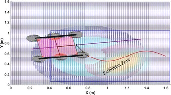
. Figure 14 shows XY projection and the selection of the CG data points in the CG-Space domain to move the Rover corresponding to the sinusoidal end-effector path. The terrain used in the simulations, shown in Figs. 14, 15, and 16, is real sand terrain generated in Section 3.1, Fig. 6. The cyan points show the possible origins of manipulator base frame M
0
corresponding to the start point of the end-effector path, and the blue points are the outer CG-points overlapping with some red points. Similarly, for each point of the end-effector path
 $ee_{d}$
, we get corresponding possible manipulator base frame origins set
 . After getting those sets, we first check for a common intersection point where we can place the base so that the arm can follow the end-effector path. If such a common position does not exist, we do the least-square path search if the curvature constraint is satisfied in the common data set with X and Y coordinates.
Initial poses of the Rover Manipulator System in the CG-Space corresponding to the end-effector path. The blue rectangle indicates the actual search region; the red spots indicate the CG data points lie in the forbidden region; the cyan points show the possible location of the manipulatior arm’s base frame M0 corresponding to the starting point of the end-effector path; dark blue points show the corresponding CG data; the blue line shows the Rover path in 2D projection; and the red sinusoidal curve is the end-effector path.

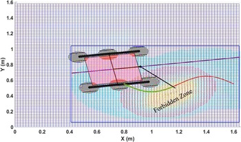
Rover path in CG-Space corresponds to the end-effector path over obstacle space. The blue rectangle indicates the actual search region; the red spots indicate the CG data points lie in the forbidden region; the cyan points show the possible location of the Rover CG corresponding to discretized points of the end-effector path; the blue line shows the Rover path in 2D projection; and the red sinusoidal curve is the end-effector path and green dots over it depicts the tracking.

Path of Rover in CG-Space corresponding to circular end-effector path. The red spots indicate the CG data points lie in the forbidden region; the cyan points show the possible location of the Rover CG corresponding to discretized points of the end-effector path; intersections of data sets are represented as blue dotted zones; the blue line shows the Rover path in 2D projection.

Such a simplified path looks straight line in 2D but is connected as a spline curve after transforming from a manipulator base frame to CG in 3D CG-Space, as shown in Fig. 15. In this figure, we consider half of the set due to symmetry along X-axis. The blue rectangle, shown in Fig. 15, indicates the actual search region, where the Rover can lie according to the minimum and maximum value of the end-effector path (X, Y) coordinates. The red spots in Figs. 15 and 16 indicate that the CG data points lie in the forbidden region caused by a high-gradient mount on the terrain. After removing such forbidden points from the combined data set to plan the base path in CG-Space, we use the least-square straight line fit in XY projection of such point cloud. This straight-line equation in the above case is
 $y_{c}=mx_{c}+c, m=0.1549, c=0.62.$
Further, this straight line is projected as a final CG-path back to CG-Space as a cubic spline curve.
For the circular arc kind of end-effector path (radius r = 0.39), as shown in Fig. 16, the near-straight-line path is not feasible. To follow such a circular end-effector path, we have to generate a similar kind of circular arc either inside or outside, depending on the curvature constraint of Rover, as described in Section 4.2. In Fig. 16, the base can not be moved within the end-effector curve due to the curvature limit violation, but we can obtain a near-circular curve with a curvature radius of 0.57 m on the outside. Sometimes, it is possible to trace the circular end-effector path without moving the Rover, where we will be able to find a non-zero set from the intersection of all sets d = 1,2,…n. The intersections of data sets
 are represented as blue dotted zones in Fig. 16. Detailed inverse kinematics calculations are provided in Section 4.2. The base Paths shown in the 2D projection (Straight line in Fig. 15 and near-circular in Fig. 16) are finally projected back to the CG-Space as a piecewise polynomial form of cubic spline curve generated using MATLAB spline() function [72].
5. Results of simulation
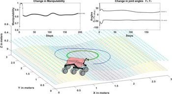
The algorithm described in Section 4 has been simulated with different end-effector paths over various terrains. The terrain data has been taken from a Kinect version 2 Depth Camera. This section shows all the simulations done so far. The desired end-effector path is given as an input to the algorithm to obtain a CG-Space-based Rover path for following the end-effector path as output. Several simulations have been performed, which are given below. The manipulability and angular change graphs are attached to each simulation result. The angular changes are presented in degrees. When the Rover changes its pose to keep the next end-effector path point within manipulator reach, the graph shows a sudden change in manipulability values on uneven terrain due to base movement. The first three figures show the circular end-effector path tracking over Flat, Sine, and SineCosine terrain in Figs. 17, 18, and 19, respectively. The green marks on the end-effector path indicate the Rover Manipulator System tracked it. The blue dotted line is the Rover path over CG-Space.
Rover Manipulator System is following a circular end-effector path over flat terrain.

Rover Manipulator System is following a circular end-effector path over sine terrain.

Rover Manipulator System is following a circular end-effector path over sine-cosine terrain.

Following the full circular end-effector path, the base need not move the complete revolution around that circular path, and at some location, base is fixed. Here, it is shown that initially, without moving the base, the arm can trace a few points on the end-effector path, and then the Rover starts moving alternatively to the arm to obtain the point over the consequent end-effector path.
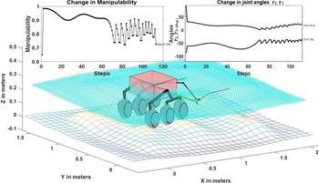
Figure 20 shows the straight-line end-effector path on a sinusoidal terrain. Further, the algorithm has been tested for three different end-effector paths: straight, sinusoidal, and polynomial curves over a rugged terrain environment. For a straight path, we get a similar straight-line movement of the Rover in terms of X and Y coordinates, which is further projected back to CG-Space in terms of a spline curve in 3D, as shown in Fig. 21. In this figure, the initial base configuration has been chosen such that the end-effector can trace maximum points on the path, as shown by the green marks on the red path line. Later, the Rover Manipulator System has to move its mobile base location to make the end-effector reachable to the rest of the end-effector points. Until the mobile base changes its location, the change in the manipulability index is smooth for rugged terrain, but it shows abrupt change when the base location is changed. Figures 22 and 23 show the results for the sinusoidal and polynomial end-effector paths on rugged terrain, respectively. The algorithm has also been tested for such types of terrain environments where there is a high-gradient zone.
Rover Manipulator System is following a straight end-effector over sine terrain.

Rover Manipulator System is following a straight end-effector over uneven terrain.

Rover Manipulator System is following sinusoidal end-effector path over uneven terrain.

Rover Manipulator System is following a polynomial curve end-effector path over uneven terrain.

Figures 24 and 25 display the full circular end-effector path simulation, which the Rover Manipulator System follows without alteration in its Rover configuration. Figure 26 depicts the straight-line end-effector path followed over a high-gradient area where the base cannot ascend. Similarly, Fig. 27 shows a simulation of a polynomial curved path over that high-gradient area, and Fig. 28 shows a simulation of a curved spiral path between two high-gradient zones.
Rover Manipulator System is following a circular end-effector path in the YZ plane over rough terrain with a high-gradient region.

Rover Manipulator System is following a circular end-effector path in the XZ plane over rough terrain with a high-gradient region.

Rover Manipulator System is following a straight end-effector path over rough terrain with high-gradient region.

Rover Manipulator System is following a polynomial end-effector path over rough terrain with high-gradient region.

Rough terrain with two high-gradient regions and the Rover Manipulator System is following a curved spiral end-effector path.

6. Experimental setup
The end-effector tracking of the wheel mobile manipulator system has been experimentally evaluated on uneven terrains made of rock and sand. Currently, the terrain bed has a size of 1.65 m × 1.6 m (Fig. 15). The scanned terrain data using the Kinect V2 sensor was converted into mesh-grid form for simulation purposes and CG-Space generation. The mobile base of the system contains ten motors for movement (six drive Maxon motors with specification EC MAX 30, 40 W, 12 V DC and four steering motors with specification EC MAX 32, FLAT MOTOR, 15 W, 12 V DC). Each motor has an EPOS motor controller connected to a central PC (Intel Core i5).
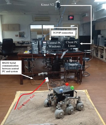
The central PC runs the motor control program written in C++ using the EPOS controller’s command library. Further, the TCP/IP connection communicates between the central and client PCs (Intel dual-core processors). The client PC runs the program to estimate the pose of the Rover Manipulator System using the Kinect sensor. The wheel velocities of the mobile base, steering angles, and joint angles of the manipulator are sent to the central PC from the client PC for end-effector path tracking. Figure 29 shows the real image of the experimental setup with a schematic diagram of the communication among the different elements of the system, that is, the Kinect V2 sensor, the client PC, and the central PC. The client PC runs on Ubuntu 14.04 operating system, and the central PC runs on the Windows XP operating system. The program to extract the real-time pose measurement values using Kinect is written in C++ programing language. The program is integrated inside the ROS environment using OpenCV and Point Cloud libraries. The program for the end-effector path tracking is written in Python programing language.
A real image of the experimental setup with a schematic diagram of the communication system.

In this work, the Kinect sensor [Reference Pagliari and Pinto66] serves the dual purpose role of extracting the terrain elevation data and estimating the real-time pose of the mobile base and the end-effector of the Rover Manipulator System. The Kinect sensor captures the bird’s eye view of the Rover Manipulator System from a fixed overhead position on the top of the workspace. A marker coordinate frame (M) is defined for pose estimation, as shown in Fig. 30(a). Color-based marker detection technique is implemented here. Three colored markers (red, green, and blue) have been fixed on the top plane of the mobile base, and a separate white marker is used for tracking the end-effector pose. Kinect sensor estimates the spatial coordinate location of each marker’s center in its frame (C). The X-axis (
 $\hat{x}_{m}$
) of the marker frame (M) is in the direction of the position difference vector of the red and the green markers (Fig. 30(a)) and then normalizes the difference. Similarly, the Y-axis vector (
 $\hat{y}_{m}$
) is established. Finally, the Z-axis vector (
 $\hat{z}_{m}$
) is the normalized cross product of X-axis and Y-axis vectors. Once all three orthogonal marker frame directions are obtained, the transformation matrix from the Kinect frame to the Marker frame is calculated as a homogeneous transformation matrix
 $T_{M}^{C}=\left[\begin{array}{c@{\quad}c} r_{m} & t_{m}\\[1pt] 0 & 1 \end{array}\right]$
. The translational vector (
 $t_{m}$
) is the position vector of the green marker and the column of the rotational matrix (
 $r_{m}$
) are the orthogonal direction vectors (
 $\hat{x}_{m}, \hat{y}_{m}, \hat{z}_{m}$
). Transformation
 $T_{M}^{C}$
provides the orientation and position of marker frame M with respect to the Kinect frame (C).
(a) Tracking image captured by Kinect and displayed on ROS platform and corresponding marker frame description with four markers in a 3D model of the Rover (b) schematic diagram of different coordinate frames used to extract the pose of the mobile base and the end-effector.

The static sensor errors represent the estimation bias, which can be solved by proper calibration. Still, the dynamic sensor errors represent the variance in estimation that needs improvement by filtering methods. As the Kinect measurement has dynamic noise [Reference Pagliari and Pinto66–Reference Park, Shin, Bae and Baeg73], Kalman filtering has been implemented to extract a more accurate estimate of the position and orientation of the marker frame from the noisy sensor data. The implementation of the Kalman filter in marker frame detection is similar, as presented by Beteley et al. [Reference Teka, Raja and Dutta54].
Next, in order to obtain the transformation
 $T_{R}^{G}$
between the Rover Manipulator System instantiations frame of reference (R) and global frame (G), we have used the information, which is obtained from marker frame (M) with respect to global frame. The equation to calculate
 $T_{R}^{G}$
can be written as:
 \begin{equation}T_{R}^{G}(t)=T_{C}^{G}T_{M}^{C}(t)T_{R}^{M}\end{equation}
The schematic diagram of coordinate transformation among frames is shown in Fig. 30(b). The transformation matrix
 $T_{C}^{G}$
is obtained in Section 3.1 during terrain mapping. Matrix
 $T_{R}^{M}$
is the transformation from the marker frame (M) to the Rover Manipulator System frame (R), which provides the marker frame position and orientations in frame R.
 $T_{R}^{M}$
is fixed because the marker frame is attached to the Rover, and it is a measured quantity. However, the matrix
 $T_{M}^{C}$
changes with time because the Rover Manipulator System moves while the Kinect is fixed at an overhead location and obtained experimentally. Once
 $T_{R}^{G}$
(t) is obtained, the pose of the mobile base and the end-effector can be accurately estimated in real time using the frame transformations.
After getting simulated (desired) and experimentally followed (actual) end-effector paths in global frame G, the average and RMS errors are calculated using the following formula:
 \begin{equation}\text{RMSE}=\sqrt{\left(\left(x_{d}(i)-x_{0}(i)\right)^{2}+\left(y_{d}(i)-y_{a}(i)\right)^{2}+\left(z_{d}(i)-z_{a}(i)\right)^{2}\right)}\end{equation}
where
 $X_{d}=(x_{d}, y_{d}, z_{d})$
are the coordinates of the desired end-effector path, and
 $X_{a}=(x_{a}, y_{a}, z_{a})$
are the actual end-effector path coordinates obtained from the experiment. Suppose the path has n number of path nodes, then the average error while following the path is calculated by:
 \begin{equation}Avg \textit{error}=\frac{1}{n}\sum _{i=1}^{n}|(X_{a}(i)-X_{d}(i))|\end{equation}
The average error is the main parameter for wheel mobile manipulator system evaluation.
7. Experimental results
The Rover Manipulator System is designed to traverse uneven terrains as required for space exploration or rescue operations in hazardous areas. Hence, the experimental terrain arena comprises sand, small rocks, and obstacles (high-gradient regions). The Rover Manipulator System’s end-effector path tracking method using CG-Space framework has been experimentally evaluated on real sand terrain surfaces with high-gradient regions. The method provides the Rover path nodes over CG-Space corresponding to the desired end-effector path, and then path data at the CG of the Rover are converted into wheel velocity. It is quite straightforward to get the wheel velocity and steering angles using the base kinematics at each path node, described in ref. [Reference Raja, Dutta and Venkatesh74]. This section presents experimental results for the end-effector path tracking over two different terrains.
Case-1: Uneven terrain with double high-gradient region
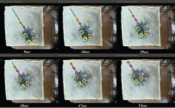
Figure 28 shows the simulation for the end-effector path tracking on this kind of terrain. In an experimental evaluation, a straight-line end-effector path is considered. Figure 31 shows the actual tracking images captured by Kinect, which shows the difference between the desired and experimental path of the end effector. Figure 32 shows the simulated and experimental path in the simulated environment with its 2D projection to better understand path deviations. Figure 33 shows the RMS error variation during different path steps.
The end-effector follows the straight-line path over an uneven terrain between two high-gradient regions (the black line shows the desired path, and the pink line shows the actual path).

(a) Tracking error between desired and actual end-effector path drawn over CG-Space of double high-gradient terrain in a simulated environment (blue line shows the Rover CG-path), (b) deviation of actual end-effector path from the desired path in 2D visualization.

RMS error at each step while following an end-effector path between two high-gradient regions.

The average error between the desired and actual end-effector path followed by the Rover Manipulator System during this experiment is 0.0093 m.
Case-2: Uneven terrain with a single high-gradient region
Figures 24– 27 show different end-effector path-tracking simulations on this kind of terrain. An experimental evaluation considers a straight-line end-effector path over a high-gradient region. Figure 34 shows the actual tracking images captured by Kinect, which shows the difference between the desired and experimental path of the end effector.
The end-effector tracks the straight-line path over high-gradient regions of the rough terrain (the black line shows the desired path, and the pink line shows the actual path).

Figure 35 shows the simulated and experimental path in the simulated environment with 2D path projections. Figure 36 shows the RMS error at each path step. Here, the deviation is more when the Rover reaches near the high-gradient mount to follow the desired path.
(a) Tracking error between simulated and actual end-effector path drawn over CG-Space of single high-gradient terrain in a simulated environment (blue line shows the Rover CG-path), (b) deviation of actual end-effector path from the desired path in 2D visualization.

RMS error at each step while following an end-effector path over a high-gradient region.

The average error between the desired and actual end-effector path followed by the Rover Manipulator System during this experiment is 0.02565 m.
8. Comparison with other methods
The main aim behind the proposed approach is to develop a real-time end-effector path-tracking framework with the help of the CG-Space concept. The pose of the Rover can be calculated in real-time according to the end-effector path by solving manipulator arm inverse kinematics between end-effector task space and CG-Space. The computational overhead in terms of simulation time to generate the mobile base path (which is the path of the Rover in this work) according to the end-effector path is provided and also compared with other existing methods as mentioned below:
The average time taken by the proposed method to generate the Rover path according to the different desired end-effector paths and terrain conditions is mentioned below and also summarized in Table IV:
Comparison of average path generation time among various methods available in the literature.

-
1. The straight-line end-effector path takes an average of 0.774 s, while the Rover moves over flat, sine, sin-cosine, or rough terrain.
-
2. The circular end-effector path takes an average of 0.964 s for even terrain (flat, sine, sin-cosine)
-
3. The circular end-effector path takes an average of 1.203 s for uneven terrain.
The performance of other methods is discussed below:
-
1. ALM [Reference Raja, Dasgupta and Dutta12] based optimization took 10–15 min to calculate the whole mobile-manipulator pose corresponding to just a single point on the end-effector path and also suffered with significant simulation error (around 0.2 m)
-
2. In the case of KSOM-based [Reference Raja, Dutta and Dasgupta51–Reference Raja, Dutta and Dasgupta53] redundancy resolution and path planning methods, the authors mentioned that it takes several hours to learn the terrain for the KSOM network and then generate the path. They just achieved accuracy in simulations as the error in simulation reduced to 0.005 m.
-
3. While using a dual-KSOM network (Teka et al. [Reference Teka, Raja and Dutta54]), training took 9 h of runtime on MATLAB.
The above three methods were used for the same type of Rover Manipulator Systems. However, a few more end-effector trajectory tracking methods have been mentioned for better comparison, but all worked in 2D, where the mobile base moved on flat ground.
-
1. Bidirectional PSO optimization [Reference Ram, Pathak and Junco58] took average simulation time of 657, 538, and 3648 s in circular, Bezier, and rectangular end-effector trajectories, respectively, while the base moves on flat terrain.
-
2. Conventional PSO optimization for 7 DOF mobile manipulator mounted on a two-wheeled differential mobile platform [Reference Khan, Li, Chen and Liao62] takes 375, 488, and 468 s for circular, rectangular, and Rhodonea end-effector trajectories, respectively, while moving on flat ground.
-
3. The BAORNN algorithm by Khan et al. [Reference Khan, Li, Chen and Liao62] takes 4.9, 4.05, and 3.26 s for the same three cases of circular, rectangular, and Rhodonea end-effector trajectories, respectively, while moving on flat ground.
-
4. Xing et al. [Reference Xing, Gong, Ding, Torabi, Chen, Gao and Tavakoli27] used AMoMDi-framework for motion accuracy of flat terrain mobile manipulator and took 10.8 s to complete a circular end-effector trajectory.
The average errors in the experimental evaluations (as shown in Table V.) are less than the results obtained by the standard KSOM [Reference Kohonen50], modified KSOM-based inverse kinematics of a redundant mobile manipulator by Rekha et al. [Reference Raja, Dutta and Dasgupta53] and Teka et al. [Reference Teka, Raja and Dutta54], even without implementing any tracking control scheme. The main reason behind less error during experimental evaluation using CG-Space-based end-effector path-tracking method is that the mobile base does not move until the arm can track the desired end-effector path within the manipulability bound.
Comparison of experimental errors among various methods available in the literature.

9. Conclusions
The proposed method provides a novel way to find the Rover path in CG-Space coupled with the end-effector path in task space instead of resolving the redundancy of the Rover Manipulator System. This work deals with the arm’s inverse kinematics for a highly redundant 14 DOF Rover Manipulator System moving in CG-Space. Such a system is well-designed for traversing rough terrain and following the end-effector path even over a high-gradient region where the Rover cannot traverse. The method can be implemented when two subsystems do task coordination together on rough terrain. Here, the end-effector task space is mapped back to CG-Space using a simple 3-link IK solution, and we will get the base path in 3D Cartesian space using a 6D joint-angle space of the Rover. While solving IK for arm, the algorithm is also satisfying manipulability constraints. Rover will not move if the manipulator arm tracks the path within the manipulability bound.
The KSOM-based algorithms give a unique solution for redundancy resolution problems, which is not desirable sometimes. Fuzzy-KSOM can solve such issues, but it is computationally too expensive to implement in real-time. So there is a requirement of coupling between the end-effector path and mobile base path in a more straightforward way to achieve in real-time.
The efficacy of the proposed approach is checked through various simulations and experiments, which show that the proposed method performs better than the KSOM and optimization-based methods in terms of time to get the desired base path. The main advantage is that we do not have any simulation error as the 3-link inverse kinematics give the unique solution for each end-effector path point between the CG-Space and the end-effector space while following the path. Once the Rover path is found in the CG-Space corresponding to the end-effector path, the next part is to move the Rover whenever its manipulator arm cannot follow the desired end-effector path within the manipulability bound. This method can avoid obstacles and high-gradient regions by invalidating the corresponding CG data points while searching for the Rover path in CG-Space. So it is adaptive enough to handle the dynamic change in free space and obstacle space. However, this framework has a future scope with dynamic obstacle avoidance. Since no slipping and skidding is considered during simulation, slippage and wheel sinking models can be incorporated in future work.
Authors’ contributions
Both authors contributed to this research. This paper has two authors. Authors’ names and contributions to the paper are Shubhi Katiyar (Terrain mapping, simulation environment modeling, base path selection over CG-Space, end-effector path tracking, inverse kinematics between end-effector task space and CG-Space, simulations for different end-effector paths over various terrains, and conclusions), Prof. Ashish Dutta (planning and directing the research on CG-Space-based end-effector path tracking, simulation environment modeling, simulation study, and reviewing and editing the whole pape).
Funding
Ms. Shubhi Katiyar has received a scholarship from Visvesvaraya PhD. Fellowship from the Ministry of Electronics & Information Technology (Unique Awardee Number is MEITY-PHD-1779) during this research work.
Competing interests
The authors have no competing interests to declare that are relevant to the content of this article.
Ethics approval
Not applicable.
Consent to participate
Not applicable.
Consent for publication
All authors agree to publish the article.
Availability of data and materials
Not applicable.
Code availability
Not applicable.